Density wave propagation in a two-dimensional random dimer potential: from a single to a bipartite square lattice

Abstract

We study the propagation of a density perturbation in a weakly interacting boson gas confined on a lattice and in the presence of square dimerized impurities. Such a two-dimensional random-dimer model (2D-DRDM), previously introduced in [Capuzzi et al., Phys. Rev. A 92, 053622 (2015)], is the disorder transition from a single square lattice, where impurities are absent, to a bipartite square lattice, where the number of impurities is maximum and coincides with half the number of lattice sites. We show that disorder correlations can play a crucial role in the dynamics for a broad range of parameters by allowing density fluctuations to propagate in the 2D-DRDM lattice, even in the limit of strong disorder. In such a regime, the propagation speed depends on the percentage of impurities, interpolating between the speed in a single monoperiodic lattice and that in a bipartite one.

I Introduction

Disordered two-dimensional (2D) systems in the absence of interactions and disorder correlations are insulating, as demonstrated in the seminal work on the scaling theory of localization by Abrahams, Anderson, Licciardello and Ramakrishnan Abrahams et al. (1979). The concept of correlations for a random potential $V(r)$ is related to the behaviour of the correlation function $\overline{V(r)V(r^{\prime})}=f(r-r^{\prime})$ averaged over all the disorder configurations, where the absence of correlations corresponds to $f(r-r^{\prime})=\delta(r-r^{\prime})$. However, like disorder, potential correlations and interactions are almost unavoidable in physics, breaking the validity of the scaling theory Abrahams et al. (1979); Anderson et al. (1980); Thouless (1982). In particular, it is well established that short-range correlations, i.e. those with $f(r-r^{\prime})\rightarrow 0$ for $|r-r^{\prime}|$ greater than few lattice spacings, can induce delocalized states Hilke (1994, 2003); Capuzzi et al. (2015); Naether et al. (2015) or states that are extended over large distances Kuhn et al. (2007); Miniatura et al. (2009); while long-range correlations may cause the absence of localization Moura et al. (2004); dos Santos et al. (2007); Moura and Domínguez-Adame (2008); Moura (2010). Interactions can induce a glass-superfluid transition Fisher et al. (1989) or induced many-body localization at finite temperature Basko et al. (2006, 2007); Fleury and Waintal (2008). Moreover, for weakly interacting systems, correlated disorder can shift the onset of superfluidity Pilati et al. (2010); Plisson et al. (2011); Allard et al. (2012); Carleo et al. (2013), or enhance superfluidity itself, even in the presence of strong disorder Capuzzi et al. (2015). This has been shown for the two-dimensional Dual Random Dimer Model (2D-DRDM) Capuzzi et al. (2015), that, analogously to the well-known one-dimensional (1D) model Dunlap et al. (1990); Schaff et al. (2010); Larcher et al. (2013), is a tight-binding model characterized by correlated impurities that become “transparent”at a given resonance energy, like identical Fabry-Perot cavities. If the Hamiltonian parameters are tuned so that the resonance energy matches the ground-state energy, the ground state is not affected by the disorder, even in the presence of weak interactions. The density homogenization induced by the resonance drives the superfluid fraction Capuzzi et al. (2015). This happens at the ground-state energy, but, as soon as the system is perturbed, higher energy states are involved, and it is not straightforward to derive the response of the system. Indeed, strictly-speaking, the resonant energy in the absence of interactions is only one (or few Larcher et al. (2013)), so that all the other states with different energy should be localized, even if a part of them ($\mathcal{N}^{1/2}$ in 1D, $\mathcal{N}$ being the number of states Dunlap et al. (1990)) is expected to be localized on the entire system length.

In this work we study the transport of an initial ring-shaped density perturbation in a weakly interacting boson gas confined on a 2D-DRDM lattice, and we compare it with the case of a fully uncorrelated random lattice (UN-RAND). We analyze both the shape of the perturbation and its propagation speed as a function of the disorder properties. Far from the resonance condition, the density fluctuation distorts as it travels through the lattice irrespective of the model disorder. However, close to the resonance condition, in the 2D-DRDM, the density perturbation travels through the system without broadening and with a well-defined speed. The propagation speed depends on the percentage of impurities and its value is between the speed of a density perturbation in a single square monoperiodic (MP) lattice and that in a bipartite (BP) one composed by two interlacing square sublattices. This shows that the main role of “resonant”random dimer impurities in a MP lattice or vacancies in a PB one is to drive the value of the propagation speed during the transport of a density excitation.

The paper is organized as follows. In Sec. II we review the features of the 2D-DRDM, including the location of the single-particle energy resonance and its effect on the spectral function for non-interacting particles. The results for the density wave propagation in a weakly interacting many-particle system are presented in Sec. III. In this section, we compare the numerical results obtained via the dynamical equations using a Gutzwiller approach, with the speed for a density perturbation in a MP lattice and a BP one, obtained within a Bogoliubov approach strictly valid for a pure Bose-Einstein condensate. We show that when the resonance condition is fulfilled, there is a well-defined speed for the density propagation and that the density wave packet is not broadened by the disorder during its propagation. Concluding remarks and perspectives are given in Sec. IV.

II The system

The 2D-DRDM is a single-particle tight-binding model, characterized by “isolated” on-site impurities that locally modify the hopping probability (middle panel of Fig. 1). The sites are arranged in a two-dimensional square lattice of size $L\times L$ and spacing $a$. The system is described by the Hamiltonian in the site basis $\{|i\rangle\}$

$$H=-\sum_{\langle ij\rangle}t_{ij}(|i\rangle\langle j|+|j\rangle\langle i|)+\sum_{i=1}^{N}\varepsilon_{i}|i\rangle\langle i|,$$ (1)

where $N=L^{2}$ is the number of sites and $\langle ij\rangle$ denotes the sum over first-neighbor sites. Here, $\varepsilon_{i}$ are the on-site energies that can be 0 or $\Delta$ in the absence or presence of an impurity, respectively, and $t_{ij}$ are the first-neighbor hopping terms that can take two values: $t$ between two empty sites and $t^{\prime}$ between an empty site and a site hosting an impurity. The fact that the impurities cannot be next-neighbours introduces short-range correlations in the disorder. Such a potential could be realized by dipolar impurities pinned at the minima of a lattice potential Larcher et al. (2013). If the percentage $p$ of impurities is zero, the lattice is MP with site energies equal to 0 and all hopping parameters equal to $t$ (left panel of Fig. 1), while if $p=0.5$, the lattice is BP with the site energies 0 and $\Delta$ distributed in a checkerboard configuration and all hopping parameters equal to $t^{\prime}$ (right panel of Fig. 1). More impurities cannot be accommodated in the 2D-DRDM lattice so that $p=0.5$ is the maximum value that can be attained. Furthermore, since impurities and vacancies have the same role, the most disordered configuration corresponds to the middle region, at $p=0.25$.

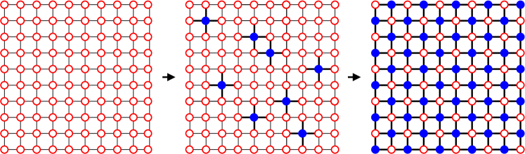
Figure 1: Schematic representation of the 2D-DRDM (middle panel) as the disordered interpolation between the monoperiodic 2D lattice (left panel) and the bipartite one (right panel).

Therefore, by varying $p$ the 2D-DRDM lattice can be seen as a disorder-mediated crossover between a MP and a BP lattice.

With the aim to understand the role of the impurity structure, one can focus on the case of a single impurity in the lattice. Let’s call $B$ the subspace defined by the impurity and $A$ the remaining lattice subspace, composed by the remaining $N-1$ lattice sites. We have previously shown in Ref. Capuzzi et al. (2015) that it exists an energy $E_{\text{res}}$ where the Green’s function in the $A$ subspace, $G_{A}(E)=\langle A|(E-H)^{-1}|A\rangle$, is the same in the presence and in the absence of an impurity. This implies that the impurity becomes “transparent” at this resonance energy $E_{\text{res}}$ fulfilling

$$\dfrac{t^{2}}{E_{\text{res}}}=\dfrac{(t^{\prime})^{2}}{E_{\text{res}}-\Delta}.$$ (2)

Therefore, at the energy $E_{\text{res}}=-t^{2}\Delta/((t^{\prime})^{2}-t^{2})$, the system is not perturbed by the presence of the impurities so that states remain delocalized over the whole system. In the case of the 1D DRDM, it was shown in Dunlap et al. (1990) that the number of states that are unperturbed and extended over the entire system scales as $\sqrt{N}$. Such a behavior can also be expected to occur for states around $E_{\text{res}}$ in the 2D-DRDM as confirmed in Fig. 2 where we plot the disorder-averaged spectral function $\mathcal{A}(\boldsymbol{k},e)$ defined by

$$\mathcal{A}(\boldsymbol{k},e)=\overline{\langle\boldsymbol{k}|\delta(H-e)|\boldsymbol{k}\rangle},$$ (3)

where $\overline{\cdots}$ denotes the average over different disorder realizations and $|\boldsymbol{k}\rangle$ is a momentum eigenstate. Hereafter, in our numerical calculations we shall consider a square lattice with side $L=50$, totaling $N=2500$ sites, and open boundary conditions. The results depicted in Fig. 2 correspond to 100–500 realizations of the disorder with a percentage $p=0.25$. The spectral function $\mathcal{A}(\boldsymbol{k},e)$ is essentially nonzero along the average dispersion relation

$$\langle e\rangle(\boldsymbol{k})=\dfrac{\int\mathcal{A}(\boldsymbol{k},e)\,e\,{\rm d}e}{\int\mathcal{A}(\boldsymbol{k},e)\,{\rm d}e},$$ (4)

but its spread in energy strongly depends on the resonance condition. As shown in Fig. 2, the spectral density is well represented by a single energy peak at $\langle e\rangle(k)$ only around $E_{\text{res}}$ : $E_{\text{res}}=-0.55t$ for $\Delta=0.44t$ (first panel of Fig. 2), $E_{\text{res}}=-1.25t$ for $\Delta=10t$ (second panel), $E_{\text{res}}=-2.5t$ for $\Delta=20t$ (third panel), and $E_{\text{res}}=-4t$ for $\Delta=32t$ (fourth panel).

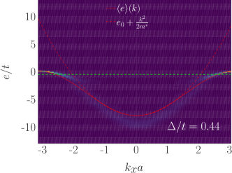
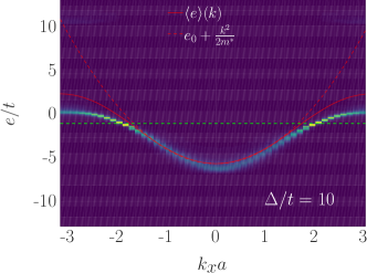
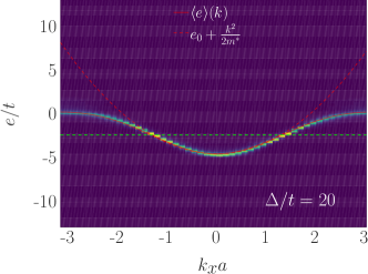
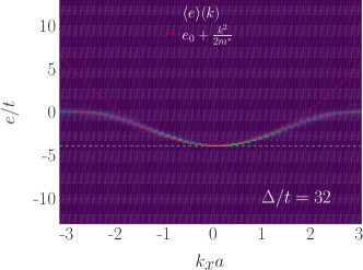
Figure 2: Disorder-averaged spectral function $\mathcal{A}(\boldsymbol{k},e)$ for a 2D-DRDM square lattice with $t^{\prime}=3t$, $p=0.25$ and $k_{y}=0$ as a function of $k_{x}$ for several values of $\Delta$. The horizontal dashed lines mark the resonance energies $E_{\text{res}}$. Continuous red lines correspond to $\langle e\rangle(\boldsymbol{k})$, [Eq. (4)] and the dashed red lines correspond to a quadratic fitting. The different panels correspond to $\Delta/t=0.44$, 10, 20 and 32.

By choosing the resonance energy at the ground-state energy $E_{\text{GS}}^{\text{MP}}$, namely, at the bottom of the energy band ($k=0$), the energy excitations become largely unaffected by the disorder and therefore one could expect that the long wavelength density perturbations, i.e. the sound waves, in a weakly interacting system will be well defined. The condition $E_{\text{res}}=E_{\text{GS}}^{\rm MP}$, $E_{\text{GS}}^{\rm MP}=-4t$ being the MP ground-state energy, sets the value of $\Delta$ as a function of $t^{\prime}$ and $t$:

$$\Delta_{\text{res}}=4t[(t^{\prime}/t)^{2}-1].$$ (5)

It is worthwhile noticing that if $\Delta=\Delta_{\text{res}}$, the MP ground-state energy, $E_{\text{GS}}^{\rm MP}=-4t$, and the BP one, $E_{\text{GS}}^{\rm BP}=\frac{1}{2}[\Delta-\sqrt{\Delta^{2}+64(t^{\prime})^{2}}]$ coincide. Indeed, one could start from the BP lattice, and introduce the disorder as vacancies, the 2D-DRDM being a disordered BP lattice. By calculating the Green’s function in the presence and in the absence of a single vacancy, and by imposing that $E=E_{\text{GS}}^{\rm BP}$, one obtain exactly the same resonance condition (5). In the presence of weak interactions, we have previously shown that the resonance is shifted to lower values of $\Delta$ Capuzzi et al. (2015) and it is accompanied by a minimization of the density fluctuations and enhancement of the superfluid fraction.

III Density wave propagation

In order to describe the propagation of a density fluctuation we include interactions into the system. An interacting boson gas confined in an optical lattice can be described by the Bose-Hubbard Hamiltonian, which in the grand canonical ensemble reads

$$H_{\text{BH}}=-\sum_{ij}t_{ij}(\hat{a}_{i}^{\dagger}\hat{a}_{j}+\hat{a}_{j}^{\dagger}\hat{a}_{i})-\sum_{i}(\mu-\varepsilon_{i})\hat{n}_{i}\\ +\dfrac{U}{2}\sum_{i}\hat{n}_{i}(\hat{n}_{i}-1),$$ (6)

where $\hat{a}_{i}^{\dagger}$ is the creation operator defined at the lattice site $i$ and $\hat{n}_{i}=\hat{a}_{i}^{\dagger}\hat{a}_{i}$. As in the case of the single-particle model, the hopping parameters $t_{ij}$ are chosen to describe either the 2D-DRDM or the UN-RAND lattice. The parameter $U$ is the interparticle on-site interaction strength, and $\mu$ denotes the chemical potential fixing the average number of bosons. We study the dynamics governed by the Hamiltonian (6) using the time-dependent Gutzwiller ansatz for the wave function Rokhsar and Kotliar (1991); Krauth et al. (1992); Jaksch et al. (1998)

$$|\Phi(\tau)\rangle=\prod_{i}^{L\times L}\sum_{n_{i}}f_{i}(n_{i},\tau)|n_{i}\rangle,$$ (7)

where $f_{i}(n,\tau)$ is the probability amplitude of finding $n$ particles on site $i$ at time $\tau$. The Gutzwiller approach has been previously used to describe the superfluid-insulator transition and the stability of bosons in an optical lattice with and without random local impurities Altman et al. (2005); Buonsante et al. (2009); Powell et al. (2011). It allows interpolating between the deep superfluid and the Mott insulating regimes. The dynamical equations obeyed by the amplitudes $f_{i}(n,\tau)$ can be obtained variationally by extremizing the action $\mathcal{S}\left\{f_{i}(n,\tau),f_{i}^{*}(n,\tau)\right\}=\int_{\tau_{1}}^{\tau_{2}}d\tau\mathcal{L}$, with

$$\mathcal{L}=\frac{i\hbar}{2}\left(\langle\Phi(\tau)|\dot{\Phi}(\tau)\rangle-\langle\dot{\Phi}(\tau)|\Phi(\tau)\rangle\right)-\langle\dot{\Phi}(\tau)|H_{\text{BH}}|\dot{\Phi}(\tau)\rangle.$$ (8)

Such a procedure allows us to study the time evolution of the system at an affordable computational cost. However, being a grand canonical description, there is no guarantee that the expectation value of the number operator will remain constant in time. In our calculations, we have verified that particle conservation occurs typically with a relative accuracy of $10^{-4}$, so that more demanding number conserving approaches Schachenmayer2011 ; Peotta2013 ; Shimizu2018a are not needed.

To probe the effect of the disorder correlations on the transport properties we excite a density wave at the center of the lattice and study its propagation. Such a density wave is constructed by solving the stationary problem of the disordered system subject to an additional Gaussian potential that shifts the on-site energies $\varepsilon_{i}$ by

$$V_{i}=Ae^{-r_{i}^{2}/2\sigma^{2}}$$ (9)

where $\mathbf{r}_{i}$ is the position of site $i$, $A$ is the amplitude and $\sigma$ the width of the perturbing potential. We shall consider negative $A$ values that create a dip in the confinement which in turn induces a density bump at the lattice center of the form $\delta n=\delta n_{0}e^{-r_{i}^{2}/{{\tilde{\sigma}}^{2}}}$. The amplitude $\delta n_{0}$ and the width $\tilde{\sigma}$ depend not only on $V_{i}$, but also on the disorder configuration. Once the density bump is created, the additional Gaussian potential is turned off and the system is let to evolve subject to the disordered potential. In a circularly symmetric setup without any disorder, the initial density bump would lead to a propagation of a ring-shaped fluctuation characterized by its mean radius and transverse section. The evolution of the mean radius measures the propagation speed and the size of the transverse section, its broadening. However, since the different momenta components scatter with the disorder at different speeds and interfere with each other, the evolution of the density perturbation become more complex, and the shape of the initial ring may be lost. Therefore, the evolution will be mainly characterized by the propagation speed and broadening of the angularly averaged density fluctuation.

In Fig. 3 we compare the time evolution of a density perturbation in an UN-RAND lattice and in a 2D-DRDM one for $t^{\prime}=3t$, different values of $\Delta$ and $p=0.25$. We consider a system with a weak interaction $U/t=10^{-2}$ and average number of particles per site $\langle n_{i}\rangle=5$ Capuzzi et al. (2015). For any value of $\Delta$ in the UN-RAND model, the density perturbation distorts as it moves through the system; whereas in the 2D-DRDM, if $\Delta$ is close to the resonant value $\Delta_{\text{res}}=32t$, the density perturbation propagates for a long time without a pronounced dispersion. This well-defined long-time density propagation indicates that the density packet is not strongly deformed by the disorder during its motion.

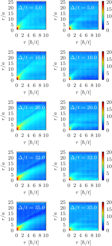
Figure 3: Time evolution of the angularly averaged density $n(r,t)$ for an initial perturbation with $\sigma/a=1$ and $A/t=-5$ for different values of $\Delta$ for the case of a 2D-DRDM lattice (left column) and of a UN-RAND system (right column). Each depicted density is obtained by averaging the density over 30 disorder realizations with $p=0.25$ for each model.

The deformation can be quantified by calculating the root-mean-square (RMS) and the angular variance of the propagating density fluctuations. The RMS is calculated as $\mathrm{RMS}=\sqrt{\langle r^{2}\rangle-\langle r\rangle^{2}}$ where the spatial averages are taken over the disorder-averaged fluctuations $\overline{\delta n}$ as $\langle F(r)\rangle=\int F(r)\overline{\delta n}^{2}/\int\overline{\delta n}^{2}$. On the other hand, the angular variance is computed as $\mathrm{var}_{\phi}(\delta n)=\sqrt{\int d\phi\,\delta n(\phi)^{2}-\left(\int d\phi\,\delta n(\phi)\right)^{2}}$ for the density perturbation $\delta n(\phi)$ evaluated at the radius corresponding to the location of the density peak. These magnitudes are measured at a fixed final time of $\tau=9\hbar/t$ and shown in Figs. 4 and 5, respectively, as functions of $\Delta$ for two values of the interaction strength: $U/t=10^{-1}$ (full symbols) and $U/t=10^{-2}$ (empty symbols). The results in a 2D-DRDM and UN-RAND lattice at $p=0.25$ are depicted in circles and squares, respectively.

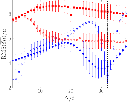
Figure 4: RMS of average density perturbation for different values of $\Delta$ at time $\tau=9\hbar/t$, for the cases $U/t=10^{-2}$ (empty symbols) and $U/t=10^{-1}$ (full symbols). Circles correspond to the 2D-DRDM model and squares to an UN-RAND one, both at $p=0.25$. The vertical dashed line indicates $\Delta_{\rm res}$.

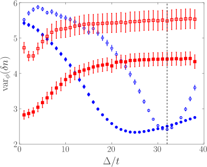
Figure 5: Average angular variance of a density perturbation for different values of $\Delta$ at time $\tau=9\hbar/t$, for the cases $U/t=10^{-2}$ (empty symbols) and $U/t=10^{-1}$ (full symbols). Circles correspond to the 2D-DRDM model and squares to an UN-RAND one, both at $p=0.25$. The vertical dashed line indicates $\Delta_{\rm res}$.

For the case of the UN-RAND disorder, both these quantities are weakly dependent on $\Delta$, while for the case of the 2D-DRDM disorder they display a sharp minimum when the density perturbation remains well-defined and does not spread out. The position of the minimum depends on the interaction strength: it corresponds to $\Delta\simeq\Delta_{\text{res}}$ for the very weakly interacting gas and moves to lower values by increasing the interactions Capuzzi et al. (2015). It is worthwhile noticing that given the finite size of the system representing experimental setups, it is not possible to perform a detailed study of the long-time evolution of the RMS, and thus to unambiguously distinguish between a wave-type and a diffusive dispersion.

III.1 Propagation in MP and BP lattices

Aiming to understand the density perturbation propagation in the disordered 2D-DRDM lattice, we study the dynamics in the MP and BP lattices. The 2D-DRDM can be seeing as a MP lattice with dimerized impurities or as a BP lattice with vacancies. Analytical expressions for the sound speed can be obtained if the gas is a pure Bose-Einstein condensate (BEC). The BEC limit corresponds to on-site coherent states with Poissonian probability distribution in the Gutzwiller ansatz

$$|\Phi_{\text{BEC}}\rangle=\prod_{i}^{L\times L}\sum_{n_{i}}f_{i}(n_{i})|n_{i}\rangle=\prod_{i}^{L\times L}\sum_{n_{i}}e^{-|\phi_{i}|^{2}/2}\dfrac{\phi_{i}^{n_{i}}}{\sqrt{n_{i}!}}|n_{i}\rangle,$$ (10)

where $n_{i}=|\phi_{i}|^{2}$ is the on-site density, and $\phi_{i}$ is the condensate wave function at site $i$. In this case, the total energy of the BEC reads

$$E=-\sum_{i}(\mu-\varepsilon_{i})|\phi_{i}|^{2}-\sum_{\langle ij\rangle}t_{ij}\phi_{i}\phi_{j}^{*}+\dfrac{U}{2}\sum_{i}|\phi_{i}|^{4}-\dfrac{UN}{2}.$$ (11)

which gives rise to the equation of motion

$$i\hbar\dfrac{\partial\phi_{i}}{\partial\tau}=\dfrac{\partial E}{\partial\phi_{i}^{*}}=-\sum_{i}(\mu-\varepsilon_{i})\phi_{i}-\sum_{\langle ij\rangle}t_{ij}\phi_{j}\\ +2U\sum_{i}|\phi_{i}|^{2}\phi_{i}.$$ (12)

The low-amplitude dynamics of the gas is governed by the collective excitations of the system. These are calculated through linearization of the equation of motion (12) around a stationary solution $\phi_{i}^{0}$ by setting $\phi_{i}(t)=e^{-i\lambda\tau/\hbar}(\phi_{i}^{0}+u_{i}e^{i\omega\tau}+v_{i}^{*}e^{-i\omega\tau})$ where $u_{i}$ and $v_{i}$ are the amplitudes of the perturbation at site $i$ and $\omega$ the corresponding frequency. The density fluctuation can thus be written in terms of the collective mode $(u_{i},v_{i})$ as $\delta n_{i}(t)=|\phi_{i}(t)|^{2}-|\phi_{i}^{0}|^{2}\simeq 2\mathop{\mathrm{Re}}\left[e^{i\omega t}(\phi_{i}^{0}u_{i}+v_{i}^{*}\phi_{i}^{0})\right]$. The solution of the linearized dynamics leads to the so-called Bogoliubov-deGennes eigenvalue equations De Gennes (1999); Leggett (2001).

III.1.1 Bogoliubov spectrum in a MP lattice

For the case of a MP lattice, where $t_{ij}=t$ for first neighbors, we obtain the usual Bogoliubov-deGennes equations for the collective modes in a lattice

$$\begin{split}-\hbar\omega u_{i}=&-\mu u_{i}-t\sum_{\langle ij\rangle}u_{j}+2U\bar{n}u_{i}+U\bar{n}v_{i}\\ \hbar\omega v_{i}=&-\mu v_{i}-t\sum_{\langle ij\rangle}v_{j}+2U\bar{n}v_{i}+U\bar{n}u_{i}\\ \end{split}$$ (13)

where $\bar{n}=|\phi_{i}^{0}|^{2}=(\phi_{i}^{0})^{2}=[(\phi_{i}^{0})^{*}]^{2}$ is the density per site, and we have taken $\phi_{i}^{0}$ real. Solving the above eigenvalue problem is straightforward and one obtain the energy spectrum of the collective excitations $\hbar\omega_{k}^{\rm MP}=\pm\sqrt{E_{k}^{2}+2E_{k}U\bar{n}}$, with $E_{k}=-2t\left[\cos(k_{x}a)+\cos(k_{y}a)\right]+4t$ the usual single-particle dispersion relation in a square lattice of spacing $a$. The low-$k$ slope of the collective spectrum defines the sound speed $c_{s}^{\rm MP}=\lim_{k\rightarrow 0}\partial\omega_{k}/(\partial k)=a\sqrt{2U\bar{n}t}/\hbar$ Machholm et al. (2003); Liang et al. (2008); Krutitsky and Navez (2011).

III.1.2 Bogoliubov spectrum in a BP lattice

For the case of a BP lattice, we can divide the system into two sublattices of indices $i_{a}$, for sites hosting an impurity, and $i_{b}$, for sites without impurities. In this case, the Bogoliubov-deGennes equations read

$$\begin{split}-\hbar\omega u_{i_{a}}=&(\Delta-\mu)u_{i_{a}}-t^{\prime}\sum_{\langle ij\rangle}u_{j_{b}}+2U{n_{a}}u_{i_{a}}+U{n_{a}}v_{i_{a}}\\ \hbar\omega v_{i_{a}}=&(\Delta-\mu)v_{i_{a}}-t^{\prime}\sum_{\langle ij\rangle}v_{j_{b}}+2U{n_{a}}v_{i_{a}}+U{n_{a}}u_{i_{a}}\\ -\hbar\omega u_{i_{b}}=&-\mu u_{i_{b}}-t^{\prime}\sum_{\langle ij\rangle}u_{j_{a}}+2U{n_{b}}u_{i_{b}}+U{n_{b}}v_{i_{b}}\\ \hbar\omega v_{i_{b}}=&-\mu v_{i_{b}}-t^{\prime}\sum_{\langle ij\rangle}v_{j_{a}}+2U{n_{b}}v_{i_{b}}+U{n_{b}}u_{i_{b}}.\\ \end{split}$$ (14)

Here $n_{a}$ and $n_{b}$ are respectively the densities in each sublattice, verifying the condition $n_{a}+n_{b}=2\bar{n}$. The lowest-energy band of the excitation spectrum is straightforwardly calculated and reads

$$\begin{split}&\hbar\omega_{k}^{\rm BP}=\pm\left[\tilde{E}_{k}^{2}+8(t^{\prime})^{2}\dfrac{n_{a}^{2}+n_{b}^{2}}{n_{a}n_{b}}+8t^{\prime}U\sqrt{n_{a}n_{b}}+2\times\right.\\ &\left.\sqrt{\dfrac{(4t^{\prime}\delta n)^{2}}{n_{a}^{2}n_{b}^{2}}+\tilde{E}_{k}^{2}\left(\dfrac{8\bar{n}^{2}}{n_{a}n_{b}}\left(2(t^{\prime})^{2}+\sqrt{n_{a}n_{b}}t^{\prime}U\right)+U^{2}\right)}\right]^{1/2},\end{split}$$ (15)

where $\tilde{E}_{k}=-2t^{\prime}(\cos(k_{x}a)+\cos(k_{y}a))$ and $\delta n=n_{b}-n_{a}$. We thus find that the sound speed for the bipartite lattice reads

$$c_{s}^{\rm BP}=\frac{a}{\hbar}\sqrt{2t^{\prime}(n_{a}n_{b})^{1/2}U\,\left[1+\frac{\delta n^{2}t^{\prime}}{4\bar{n}^{2}t^{\prime}+(n_{a}n_{b})^{3/2}U}\right]}.$$ (16)

Due to the fixed average density $\bar{n}$, the sound speed in the bipartite lattice varies with $\Delta$ through the variation of $n_{a}$ and $n_{b}$. For vanishing $\Delta$ ($\delta n=0$), the expression of $c_{s}^{\text{BP}}$ reduces to that of $c_{s}^{\text{MP}}$ with $t=t^{\prime}$, while for very large $\Delta$ it goes to zero as $n_{a}$ vanishes and thus no perturbation can be transported.

III.2 Density perturbation size effects

When we excite the density wave as described above, the density fluctuation propagates through the lattice with a speed that depends on its spatial extent. For very large widths (small $k$) the propagation speed $v$ coincides with the sound speed, while for tight wave packets, larger-$k$ contributions have to be taken into account. The group velocity at any $k$ contributes with a weight determined by $\delta n(k)$, the density fluctuation in momentum space. The actual propagation speed can thus be written as

$$v\simeq c^{\rm MP,BP}=\int{\rm d}{\bf k}\,\dfrac{\partial\omega_{k}^{\rm MP,BP}}{\partial k}\,\delta n(k).$$ (17)

Therefore, finite-$k$ corrections are more sizable for smaller $U$, where the dispersion curves $\omega_{k}^{\rm MP,BP}$ bend more rapidly. For the disordered lattices, the propagation speed has been extracted from the position of the largest density peak during the evolution when the dynamics is started by the Gaussian perturbation with amplitude $A/t=-0.1$, and $\sigma/a=1$. The choice of $\sigma/a=1$ is determined by the experimental request that the density perturbation has to be observable during the propagation along a finite-size lattice. The calculation of the finite-size velocities $c^{\rm MP,BP}$ in Eq. (17) have been performed for a Gaussian wave packet of width $\tilde{\sigma}$. Due to the disorder, $\tilde{\sigma}$ is usually larger than $\sigma$ and depends on the system parameter $\Delta$ and the interaction strength $U$. In Fig. 6, we compare the propagation speed $v$ of a density perturbation in a disordered 2D-DRDM lattice with $c^{\rm MP}$, $c^{\rm BP}$, $c_{s}^{\rm MP}$ and $c_{s}^{\rm BP}$ for $U/t=10^{-2}$ (top panel) and $U/t=10^{-1}$ (bottom panel). Given that for both interaction strengths $\tilde{\sigma}/a\gtrsim 2$, in the weaker interacting case $U/t=10^{-2}$, the size effects of the density perturbation are quite important and the sound velocities $c_{s}^{\rm MP}$ and $c_{s}^{\rm BP}$ largely underestimate $v$. The values of $\tilde{\sigma}$ used to calculate $c^{\text{MP}}$ and $c^{\text{BP}}$ were fixed to those observed in the simulations in MP ($p=0$) and BP ($p=0.5$) lattices, respectively, for each value of $U$. In the case of the BP lattice we have further chosen the corresponding value of $\tilde{\sigma}$ at $\Delta/t=25$. For $U/t=10^{-2}$, the density fluctuations do not propagate for $\Delta/t\lesssim 10$, consistently with the behavior of the noninteracting spectral function $\mathcal{A}$ shown in Fig. 2. For stronger interactions, the effect of the finite size of the density wave packet diminishes as the linear range of the dispersion curves $\omega_{k}$ extends to higher $k$. In this case $c_{s}^{\rm MP}$ and $c_{s}^{\rm BP}$ correctly set the scale of the data for $v$ (bottom panel of Fig. 6). As a result of the interactions, the effect of the disorder is attenuated as demonstrated by the reduction of the error bars for $\Delta/t\lesssim 10$, indicating a well-defined propagation also at low $\Delta$. This can be understood from the shift and broadening of the single-particle energy resonance discussed in Sec. II. The effects of the resonance broadening on the properties of the ground state has also been discussed in Ref. Capuzzi et al. (2015).

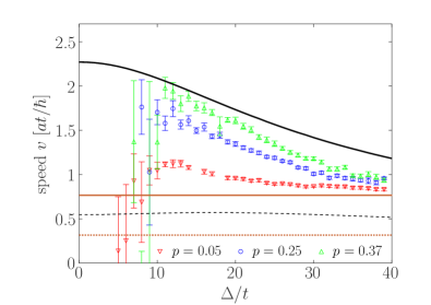
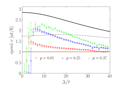
Figure 6: Speed $v$ of the density perturbation in the 2D-DRDM lattice as a function of $\Delta$ for $U/t=10^{-2}$ (top panel), and $U/t=10^{-1}$ (bottom panel). The different symbols correspond to different values of $p$. The solid black curves correspond to the BP propagation speed for $\tilde{\sigma}/a=2.2$ (see text), while solid brown curves correspond the MP propagation speed for $\tilde{\sigma}/a=2.4$ (top panel) and $\tilde{\sigma}/a=4.0$ (bottom panel). The dashed black (brown) curve corresponds to the sound speed for the BP (MP) lattice ($\tilde{\sigma}/a\rightarrow\infty$).

The variation of the propagation speed with the percentage of impurities $p$ is enlightened in more detail in Fig. 7, where we plot $v$ as a function of $p$ for $\Delta/t=25$, 32 and 40.

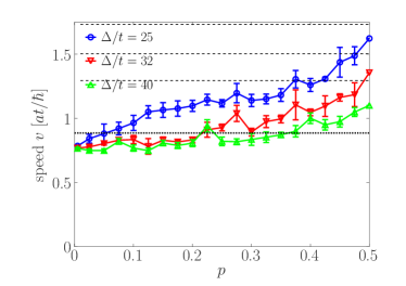
Figure 7: Speed $v$ of the density perturbation in the 2D-DRDM lattice as a function of $p$ for $\Delta/t=25,32$ and $40$. The black dotted-line corresponds to $c^{\mathrm{MP}}$ for $\tilde{\sigma}/a=2.4$, while the dashed-lines correspond to $c^{\mathrm{BP}}$ for the same values of $\Delta$ and $\tilde{\sigma}/a=2.2,2.3$ and $2.5$ for $\Delta/t=25,32$, and $40$, respectively.

The data interpolate from $c^{\rm MP}$ at $p=0$ to $c^{\rm BP}$ at $p=0.5$. From the density perturbation point of view, the 2D-DRDM lattice is like an ordered lattice in between the MP and BP lattices. The dimerized impurities are not strictly-speaking “transparent” around the resonance energy as it happens exactly at resonance. Their presence alters the propagation of density perturbations, but in the same manner as if the impurities were orderly distributed. The effect of tuning the resonance energy to the ground-state energy is that, at low-energies, the 2D-DRDM behaves like an ordered lattice interpolating the MP and the PB lattices.

IV Conclusions

In this paper we have studied the propagation of an initial ring-shaped density perturbation in a weakly interacting boson gas confined on lattice and in the presence of localized disordered impurities. If the impurities are dimerized, and their resonance energy corresponds to the ground-state energy, the density perturbation propagates essentially without spreading out. We found that the speed of the density propagation is well defined even for a tight density wave-packet (large wavevectors) and that its value depends on the percentage of the impurities $p$, ranging from the MP speed ($p=0$) to the BP one ($p=0.5$). This means that the dimerized impurities that are “transparent” at the ground-state energy, are not strictly-speaking “transparent” at energies around the resonance energy, and thus the density propagation depends on the impurities presence. The effect of the nearby resonance is that the system behaves like that the dimerized impurities were orderly distributed, for energies around the resonance energy. If the resonance is far in the spectrum, disorder correlations do not play any role, and the density wave spreads out and does not propagate any more.