Understanding the QuickXPlain Algorithm:
Simple Explanation and Formal Proof

Abstract

In his seminal paper of 2004, Ulrich Junker proposed the QuickXPlain algorithm, which provides a divide-and-conquer computation strategy to find within a given set an irreducible subset with a particular (monotone) property. Beside its original application in the domain of constraint satisfaction problems, the algorithm has since then found widespread adoption in areas as different as model-based diagnosis, recommender systems, verification, or the Semantic Web. This popularity is due to the frequent occurrence of the problem of finding irreducible subsets on the one hand, and to QuickXPlain’s general applicability and favorable computational complexity on the other hand.

However, although (we regularly experience) people are having a hard time understanding QuickXPlain and seeing why it works correctly, a proof of correctness of the algorithm has never been published. This is what we account for in this work, by explaining QuickXPlain in a novel tried and tested way and by presenting an intelligible formal proof of it. Apart from showing the correctness of the algorithm and excluding the later detection of errors (proof and trust effect), the added value of the availability of a formal proof is, e.g., (i) that the workings of the algorithm often become completely clear only after studying, verifying and comprehending the proof (didactic effect), (ii) the shown proof methodology can be used as a guidance for proving other recursive algorithms (transfer effect), and (iii) the possibility of providing “gapless” correctness proofs of systems that rely on (results computed by) QuickXPlain, such as numerous model-based debuggers (completeness effect).

1 Introduction

The task of finding within a given universe an irreducible subset with a specific monotone property is referred to as the MSMP (Minimal Set subject to a Monotone Predicate) problem [2, 3]. Take the set of clauses $S:=\{\lnot C,A\lor\lnot B,C\lor\lnot B,\lnot A,B\}$ as an example. This set is obviously unsatisfiable. One task of interest expressible as an MSMP problem is to find a minimal unsatisfiable subset (MUS) of these clauses (which can help, e.g., to understand the cause of the clauses’ inconsistency). At this, $S$ is the universe, and the predicate that tells whether a given set of clauses is satisfiable is monotone, i.e., any superset (subset) of an unsatisfiable (satisfiable) clause set is unsatisfiable (satisfiable). In fact, there are two MUSes for $S$, i.e., $\{\lnot C,C\lor\lnot B,B\}$ and $\{A\lor\lnot B,\lnot A,B\}$. We call a task, such as MUS, that can be formulated as an MSMP problem a manifestation of the MSMP problem.

MSMP is relevant to a wide range of computer science disciplines, including model-based diagnosis [4, 5, 6, 7], constraint satisfaction problems [8, 9, 10], verification [2, 11, 12, 13], configuration problems [14, 15], knowledge representation and reasoning [16, 17, 18, 19], recommender systems [20, 21], knowledge integration [22, 23], as well as description logics and the Semantic Web [6, 24, 25, 26, 27, 28]. In all these fields, (sub)problems are addressed which are manifestations of the MSMP problem. Example problems—most of them related to the Boolean satisfiability problem—are the computation of minimal unsatisfiable subsets [3, 29, 30, 31] (also termed conflicts [32, 33] or minimal unsatisfiable cores [29]), minimal correction subsets [34, 35] (also termed diagnoses [32, 33]), prime implicants [36, 37] (also termed justifications [26]), prime implicates [19, 38, 39], and most concise optimal queries to an oracle [22, 28, 40, 41].

Numerous algorithms to solve manifestations of the MSMP problem have been suggested in literature, e.g., [2, 3, 5, 8, 9, 11, 41, 42, 43, 44, 45]. For instance, the algorithm proposed by Felfernig et al. [44] addresses the problem of the computation of minimal correction subsets (diagnoses), and the one suggested by Rodler et al. [41] computes minimal oracle queries that preserve some optimality property. In general, an algorithm $A$ for a specific manifestation of the MSMP problem can be used to solve arbitrary manifestations of the MSMP problem if (i) the procedure used by $A$ to decide the monotone predicate is used as a black-box (i.e., given a subset of the universe as input, the procedure outputs 1 if the predicate is true for the subset and 0 otherwise; no more and no less), and (ii) no assumptions or additional techniques are used in $A$ which are specific to one particular manifestation of the MSMP problem.

Not all algorithms meet these two criteria. For instance, there are algorithms that rely on additional outputs beyond the mere evaluation of the predicate (e.g., certificate-refinement-based algorithms [3]), or glass-box approaches that use non-trivial modifications of the predicate decision procedure to solve the MSMP problem (e.g., theorem provers that record the axioms taking part in the deduction of a contradiction while performing a consistency check [6]). These methods violate (i). Moreover, e.g., algorithms geared to the computation of minimal unsatisfiable subsets that leverage a technique called model rotation [46] are not applicable, e.g., to the problem of finding minimal correction subsets, since there is no concept equivalent to model rotation for minimal correction subsets [3]. Thus, such algorithms violate (ii).

Among the general MSMP algorithms that satisfy (i) and (ii), QuickXPlain [9] (QX for short), proposed by Ulrich Junker in 2004, is one of the most popular and most frequently adapted. Likely reasons for the widespread use of QX are its mild theoretical complexity in terms of the number of (usually expensive) predicate evaluations required [3, 9], as well as its favorable practical performance for important problems (such as conflict [47] or diagnosis [42] computation for model-based diagnosis). In literature, QX is utilized in different ways; it is (a) (re)used as is for suitable manifestations of MSMP [14], (b) adapted in order to solve other manifestations of MSMP [5], as well as (c) modified or extended, respectively, e.g., to achieve a better performance for a particular MSMP manifestation [3], to solve extensions of the MSMP problem [41], or to compute multiple minimal subsets of the universe in a single run [43].

Despite its popularity and common use, from the author’s experience, QX appears to be quite poorly understood by reading and thinking through the algorithm, and, for most people, requires significant and time-consuming attention until they are able to properly explain the algorithm. In particular, people often complain they do not see why it correctly computes a minimal subset of the universe. This is not least because no proof of QX has yet been published.

In this work, we account for this by presenting a clear and intelligible proof of QX. The public availability of a proof comes with several benefits and serves i.a. the following purposes:

Proof Effect

(a) It shows QX’s correctness and makes it verifiable for everyone in a straightforward step-by-step manner (without the need to accomplish the non-trivial task of coming up with an own proof). (b) It creates compliance with common scientific practice. That is, every proposal of an algorithm should be accompanied with a (full and public) formal proof of correctness. This demand is even more vital for a highly influential algorithm like QX.

Didactic Effect

(a) It promotes (proper and full) understanding [48] of the workings of QX, which is otherwise for many people only possible in a laborious way (e.g., by noting down and exercising through examples and attempting to verify QX’s soundness on concrete cases). (b) It provides the basis for understanding (hundreds of) other works or algorithms that use, rely on, adapt, modify or extend QX.

Completeness Effect

It is necessary to establish and prove the full correctness of other algorithms that rely on (the correctness) of QX, such as a myriad of algorithms in the field of model-based diagnosis.

Trust and Sustainability Effect

It excludes the possibility of the (later) detection of flaws in the algorithm, and is thus the only basis for placing full confidence in the proper-functioning of QX.

Transfer Effect

It showcases a stereotypic proof concept for recursive algorithms and can provide guidance to researchers when approaching the (often challenging task of formulating a) proof of other recursive algorithms. The reason is that recursive algorithms can often be proven using a similar methodology (as ours), e.g., by showing certain invariants and using a proof by induction.

The rest of this paper is organized as follows. We discuss related work in Sec. 2, before we briefly introduce the theoretical concepts required for the understanding and proof of QX in Sec. 3. Then, in Sec. 4, we state the QX algorithm in a (slightly) more general formulation than originally published in [9], i.e., we present QX as a general method to tackle the MSMP problem. In addition, we explain the functioning of QX, and present an illustrative example using a notation that proved particularly comprehensible in our experience. The proof is given in Sec. 5, and concluding remarks are made in Sec. 6.

2 Related Work

Bradley and Manna [11] state an algorithm claimed to be equivalent to QX and give a proof of this algorithm. However, first, there is no proof that the stated algorithm is indeed equivalent to QX (which is not clear from the formulation given in [11]). Second, the proof given in [11] does not appear to be of great help to better understand QX, as the reader needs to become familiar with the notation and concepts used in [11] in the first place, and needs to map the pseudocode notation of [11] to the largely different one stuck to by Junker in the original QX-paper [9]. Apart from that, the proof in [11]—despite (or perhaps exactly because of) its undeniable elegance—is not “operation-centric” in that it is not amenable to a mental “tracking” by means of the call-recursion-tree produced by QX. In contrast, our proof is illustrative as it can be viewed as directly traversing the call-recursion-tree (cf. Fig. 1 later), while showing that certain invariant statements remain valid through all transitions in the tree, and using these invariants to prove that all (recursive) calls work correctly. Moreover, we segment our proof into small, intuitive, and easily digestible chunks, thus putting a special focus on its clarity, elucidation, and didactic value. Finally, our proof enables the verification of the correctness of the original formulation of QX. Hence, we believe that our proof is more valuable to people having a hard time understanding QX than the one in [11]. Or, to put it into the words of Hanna [50, 51], we present a proof that explains, rather one that solely proves.

3 Basics

QX can be employed to find, for an input set $U$, a minimal subset $X\subseteq U$ that has a certain monotone property $p$. An example would be an (unsatisfiable) knowledge base (set of logical sentences) $U$ for which we are interested in finding a minimal unsatisfiable subset (MUS) $X$.

Definition 1 (Monotone Property).

Let $U$ be the universe (a set of elements) and $p:2^{U}\to\{0,1\}$ be a function where $p(X)=1$ iff property $p$ holds for $X\subseteq U$. Then, $p$ is a monotone property iff $p(\emptyset)=0$ and

$$\forall X^{\prime},X^{\prime\prime}\subseteq U:\;\,X^{\prime}\subset X^{\prime\prime}\implies p(X^{\prime})\leq p(X^{\prime\prime})$$

So, $p$ is monotone iff, given that $p$ holds for some set $X^{\prime}$, it follows that $p$ also holds for any superset $X^{\prime\prime}$ of $X^{\prime}$. An equivalent definition is: If $p$ does not hold for some set $X^{\prime\prime}$, $p$ does not hold for any subset $X^{\prime}$ of $X^{\prime\prime}$ either.

In practical applications it is often a requirement that (a) some elements of the universe must not occur in the sought minimal subset, or (b) the minimal subset of the universe should be found in the context of some reference set. Both cases (a) and (b) can be subsumed as searching for a minimal subset of the analyzed set $\mathcal{A}$ given some background $\mathcal{B}$. In case (a), $\mathcal{B}$ is defined as a subset of the universe $U$ (e.g., in a fault localization task, those sentences of a knowledge base $U$ that are assumed to be correct) and $\mathcal{A}$ is constituted by all other elements of the universe $U\setminus\mathcal{B}$ (those sentences in $U$ that are possibly faulty); in case (b), $\mathcal{B}$ is some additional set of relevance to the universe (e.g., a knowledge base of general medical knowledge), whereas $\mathcal{A}$ is the universe itself (e.g., a knowledge base describing a medical sub-discipline). For example, the problem of finding a MUS wrt. $\mathcal{A}$ given background $\mathcal{B}$ would be to search for a minimal set $X$ of elements in $\mathcal{A}$ such that $X\cup\mathcal{B}$ is unsatisfiable.

Definition 2 ($p$-Problem-Instance).

Let $\mathcal{A}$ (analyzed set) and $\mathcal{B}$ (background) be (related) finite sets of elements where $\mathcal{A}\cap\mathcal{B}=\emptyset$, and let $p$ be a monotone predicate. Then we call the tuple $\left\langle\mathcal{A},\mathcal{B}\right\rangle$ a $p$-problem-instance ($p$-PI).

Definition 3 (Minimal $p$-Set (given some Background)).

Let $\left\langle\mathcal{A},\mathcal{B}\right\rangle$ be a $p$-PI. Then, we call $X$ a $p$-set wrt. $\left\langle\mathcal{A},\mathcal{B}\right\rangle$ iff $X\subseteq\mathcal{A}$ and $p(X\cup\mathcal{B})=1$. We call a $p$-set $X$ wrt. $\left\langle\mathcal{A},\mathcal{B}\right\rangle$ minimal iff there is no $p$-set $X^{\prime}\subset X$ wrt. $\left\langle\mathcal{A},\mathcal{B}\right\rangle$.

Immediate consequences of Defs. 1 and 3 are:

Proposition 1 (Existence of a $p$-Set).

1. A (minimal) $p$-set exists for $\left\langle\mathcal{A},\mathcal{B}\right\rangle$ iff $p(\mathcal{A}\cup\mathcal{B})=1$.

2. $\emptyset$ is a—and the only—(minimal) $p$-set wrt. $\left\langle\mathcal{A},\mathcal{B}\right\rangle$ iff $p(\mathcal{B})=1$.

Algorithm 1 QX: Computation of a Minimal $p$-Set

1:a $p$-PI $\left\langle\mathcal{A},\mathcal{B}\right\rangle$ where $\mathcal{A}$ is the analyzed set and $\mathcal{B}$ is the background

2:a minimal $p$-set wrt. $\left\langle\mathcal{A},\mathcal{B}\right\rangle$, if existent; ‘no $p$-set’, otherwise

3:procedure QX($\left\langle\mathcal{A},\mathcal{B}\right\rangle$)

4:    if $p(\mathcal{A}\cup\mathcal{B})=0$ then

5:         return  ‘no $p$-set’

6:    else if $\mathcal{A}=\emptyset$ then

7:         return  $\emptyset$

8:    else

9:         return ${\textsc{QX}}^{\prime}$($\mathcal{B},\left\langle\mathcal{A},\mathcal{B}\right\rangle$)     

10:procedure ${\textsc{QX}}^{\prime}$($\mathcal{C},\left\langle\mathcal{A},\mathcal{B}\right\rangle$)

11:    if $\mathcal{C}\neq\emptyset\land p(\mathcal{B})=1$ then

12:         return $\emptyset$     

13:    if $|\mathcal{A}|=1$ then

14:         return $\mathcal{A}$     

15:    $k\leftarrow\textsc{split}(|\mathcal{A}|)$

16:    $\mathcal{A}_{1}\leftarrow\textsc{get}(\mathcal{A},1,k)$

17:    $\mathcal{A}_{2}\leftarrow\textsc{get}(\mathcal{A},k+1,|\mathcal{A}|)$

18:    $X_{2}\leftarrow\textsc{${\textsc{QX}}^{\prime}$}(\mathcal{A}_{1},\left\langle\mathcal{A}_{2},\mathcal{B}\cup\mathcal{A}_{1}\right\rangle)$

19:    $X_{1}\leftarrow\textsc{${\textsc{QX}}^{\prime}$}(X_{2},\left\langle\mathcal{A}_{1},\mathcal{B}\cup X_{2}\right\rangle)$

20:    return $X_{1}\cup X_{2}$

4 Brief Review and Explanation of QX

The QX algorithm is depicted by Alg. 1. It gets as input a $p$-PI $\left\langle\mathcal{A},\mathcal{B}\right\rangle$ and assumes a sound and complete oracle that answers queries of the form $p(X)$ for arbitrary $X\subseteq\mathcal{A}\cup\mathcal{B}$. If existent, QX returns a minimal $p$-set wrt. $\left\langle\mathcal{A},\mathcal{B}\right\rangle$; otherwise, ’no $p$-set’ is output. In a nutshell, QX works as follows:

Trivial Cases: Before line 9 is reached, the algorithm checks if trivial cases apply, i.e., if either no $p$-set exists or the analyzed set $\mathcal{A}$ is empty, and returns according outputs. In case the execution reaches line 9, the recursive procedure QX’ is called. In the very first execution of QX’, the presence of two other trivial cases is checked in lines 11 and 13. (Line 11): If the background $\mathcal{B}$ is non-empty and $p(\mathcal{B})=1$, then the empty set, the only minimal $p$-set in this case (cf. Prop.1.(2)), is directly returned and QX terminates. Otherwise, we know the empty set is not a $p$-set, i.e., every (minimal) $p$-set is non-empty. (Line 13): If the analyzed set $\mathcal{A}$ is a singleton, then $\mathcal{A}$ is directly returned and QX terminates.

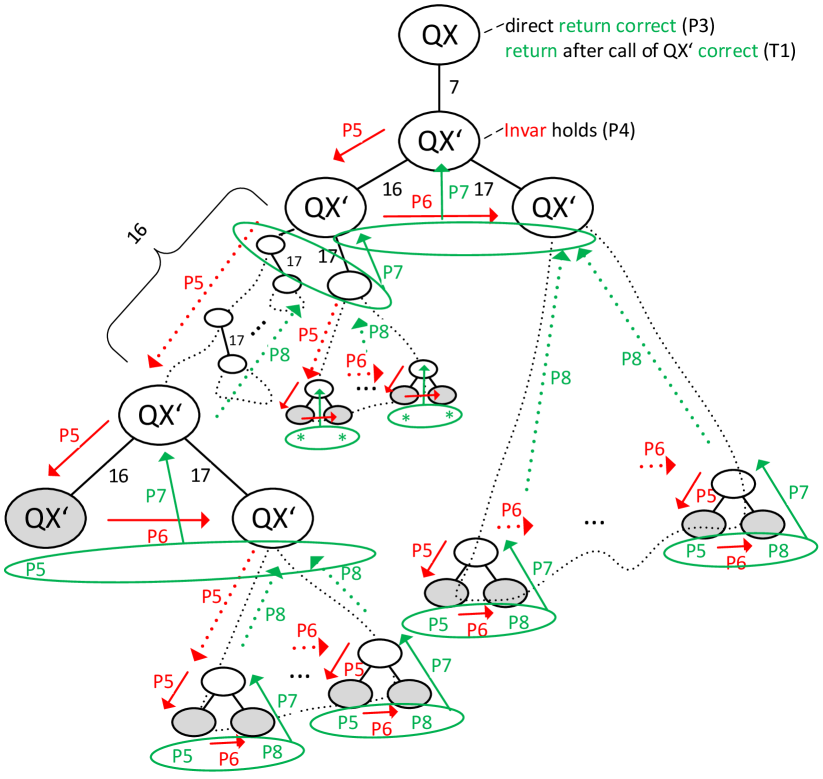
Figure 1: Call-recursion-tree produced by QX (cf. Sec. 4). The grayscale part of the figure provides a schematic illustration of the procedure calls executed in a single run of QX (where the recursion is entered, i.e., no trivial case applies). Each node (ellipse) represents one call of the procedure named within the ellipse. Edge labels (7,16,17) refer to the lines in Alg. 1 where the respective call is made. White ellipses (non-leaf nodes) are calls that issue further recursive calls (in lines 16 and 17), whereas gray ellipses (leaf nodes) are calls that directly return (i.e., in line 12 or 14). The colored part of the figure visualizes the meaning and consequences of the theorem (T1) and the various propositions (P$i$, for $i\in\{3,4,5,6,7,8\}$) that constitute the proof (cf. Sec. 5). Red arrows indicate proven propagations of the invariant property Invar (see Def. 4) between calls. Green arrows and labels indicate that respective calls return correct outputs. Start to read the colored illustrations from the top, just like QX proceeds. That is, due to P3, direct returns yield correct outputs. If QX’ is called, Invar holds by P4. If Invar holds for some call, then it is always propagated downwards to the left subtree because of P5. At the first leaf node, a correct output is returned, also due to P5. If the output of a left subtree is correct, then Invar propagates to the right subtree (P6). If the output of both the left and the right subtree is correct, then the output of the root is correct (P7). If Invar holds at the root call of some (sub)tree, then this root call returns a correct output (P8). Note how these propositions guarantee that Invar, and thus correct outputs, can be derived for all nodes of the call-recursion-tree. Intuitively, red arrows propagate Invar downwards through the tree, which then ensures correct outcomes at the leafs, from where these correct outputs enable further propagation of Invar to the right, from where the inferred correct outputs are recursively propagated upwards until the root node is reached.

Recursion: Subsequently, the recursion is started. The principle is to partition the analyzed set $\mathcal{A}=\{a_{1},\dots,a_{|\mathcal{A}|}\}$ into two non-empty (e.g., equal-sized) subsets $\mathcal{A}_{1}=\{a_{1},\dots,a_{k}\}$ and $\mathcal{A}_{2}=\{a_{k+1},\dots,a_{|\mathcal{A}|}\}$ (split and get functions; lines 15–17), and to analyze these subsets recursively (divide-and-conquer). In this vein, a binary call-recursion-tree is built (as sketched in Fig. 1), including the root QX’-call made in line 9 and two subtrees, the left one rooted at the call of QX’ in line 18 which analyzes $\mathcal{A}_{2}$, and the right one rooted at the call of QX’ in line 19 which analyzes $\mathcal{A}_{1}$. Let the finally returned minimal $p$-set be denoted by $X$, and let us call all elements of $X$ relevant, all others irrelevant. Then, the left subtree (finally) returns the subset of those elements ($X_{2}$) from $\mathcal{A}_{2}$ that belong to $X$, and the right subtree (finally) returns the subset of those elements ($X_{1}$) from $\mathcal{A}_{1}$ that belong to $X$.

• Left subtree (recursive QX’-call in line 18): The first question is: Are all elements of $\mathcal{A}_{2}$ irrelevant? Or, equivalently: Does $\mathcal{B}\cup\mathcal{A}_{1}$ already contain a minimal $p$-set, i.e., $p(\mathcal{B}\cup\mathcal{A}_{1})=1$? This is evaluated in line 11; note: $\mathcal{C}=\mathcal{A}_{1}\neq\emptyset$. If positive, $\emptyset$ is returned and the subtree is not further expanded. Otherwise, we know there is some relevant element in $\mathcal{A}_{2}$. Hence, the analysis of $\mathcal{A}_{2}$ is started. That is, in line 13, the singleton test is performed for $\mathcal{A}_{2}$. In the affirmative case, we have proven that the single element in $\mathcal{A}_{2}$ is relevant. The reason is that $p(\mathcal{B}\cup\mathcal{A}_{1})=0$, as verified in line 11 just before, and that adding the single element in $\mathcal{A}_{2}$ makes the predicate true, i.e., $p(\mathcal{B}\cup\mathcal{A}_{1}\cup\mathcal{A}_{2})=p(\mathcal{B}\cup\mathcal{A})=1$, as verified in line 4 at the very beginning. If $\mathcal{A}_{2}$ is a non-singleton, it is again partitioned and the subsets are analyzed recursively, which results in two new subtrees in the call-recursion-tree.

• Right subtree (recursive QX’-call in line 19): Here, we can distiguish between two possible cases, i.e., either the set $X_{2}$ returned by the left subtree is (i) empty or (ii) non-empty.
  Given (i), we know that $\mathcal{A}_{1}$ must include a relevant element. Reason: $\mathcal{B}\cup\mathcal{A}_{1}$ contains a minimal $p$-set (as verified in the left subtree before returning the empty set) and every $p$-set is non-empty (as verified in line 11 in the course of checking the Trivial Cases, see above). Hence, $\mathcal{A}_{1}$ is further analyzed in lines 13 et seqq. (which might lead to a direct return if $\mathcal{A}_{1}$ is a singleton and thus relevant, or to further recursive subtrees otherwise).
  For (ii), the question is: Given the subset $X_{2}$ of the $p$-set, are all elements of $\mathcal{A}_{1}$ irrelevant? Or, equivalently: Does $\mathcal{B}\cup X_{2}$ already contain a minimal $p$-set, i.e., $p(\mathcal{B}\cup X_{2})=1$? This is answered in line 11; note: $\mathcal{C}=X_{2}\neq\emptyset$ due to case (ii). In the affirmative case, the empty set is returned, i.e., no elements of $\mathcal{A}_{1}$ are relevant and the final $p$-set $X$ found by QX is equal to $X_{2}$. If the answer is negative, $\mathcal{A}_{1}$ does include some relevant element and is thus further analyzed in lines 13 et seqq. (which might lead to a direct return if $\mathcal{A}_{1}$ is a singleton and thus relevant, or to further recursive subtrees otherwise).

Finally, the union of the outcomes of left ($X_{2}$) and right ($X_{1}$) subtrees is a minimal $p$-set wrt. $\left\langle\mathcal{A},\mathcal{B}\right\rangle$ and returned in line 20.

Example 1  We illustrate the functioning of QX by means of a simple example.

Input Problem and Parameter Setting: Assume the analyzed set $\mathcal{A}=\{1,2,3,4,$ $5,6,7,8\}$, the initial background $\mathcal{B}=\emptyset$, and that there are two minimal $p$-sets wrt. $\left\langle\mathcal{A},\mathcal{B}\right\rangle$, $X=\{3,4,7\}$ and $Y=\{4,5,8\}$. Further, suppose that QX pursues a splitting strategy where a set is always partitioned into equal-sized subsets in each iteration, i.e., $\textsc{split}(n)$ returns $\lceil\frac{n}{2}\rceil$ (note: this leads to the best worst-case complexity of QX, cf. [9]).

Notation: Below, we show the workings of QX on this example by means of a tried and tested “flat” notation. In this notation, the single-underlined subset denotes the current input to the function $p$ in line 11, the double-underlined elements are those that are already fixed elements of the returned minimal $p$-set, and the grayed out elements those that are definitely not in the returned minimal $p$-set. Finally, $\scriptsize1⃝$ signifies that the tested set (single-underlined along with double-underlined elements) is a $p$-set (function $p$ in line 11 returns 1); $\scriptsize0⃝$ means it is no $p$-set (function $p$ in line 11 returns 0).

How QX Proceeds: After verifying that there is a non-empty $p$-set wrt. $\left\langle\mathcal{A},\mathcal{B}\right\rangle$ and that $|\mathcal{A}|>1$ (i.e., after the checks in lines 4 and 6 are negative, QX’ is called in line 9, and the checks in the first execution of lines 11 and 13 are negative), QX performs the following actions:

$$\mbox{\scriptsize(1)}\qquad[\underline{1,2,3,4},5,6,7,8] \;\;\;\scriptsize0⃝\quad\rightarrow\text{\quad some element of $p$-set among 5,6,7,8}$$

$$\mbox{\scriptsize(2)}\qquad[\underline{1,2,3,4,5,6},7,8] \;\;\;\scriptsize0⃝\quad\rightarrow\text{\quad some element of $p$-set among 7,8}$$

$$\mbox{\scriptsize(3)}\qquad[\underline{1,2,3,4,5,6,7},8] \;\;\;\scriptsize1⃝\quad\rightarrow\text{\quad 7 found, 8 irrelevant}$$

$$\mbox{\scriptsize(4)}\qquad[\underline{1,2,3,4},5,6,\underline{\underline{7}},{\color[rgb]{.75,.75,.75}8}] \;\;\;\scriptsize1⃝\quad\rightarrow\text{\quad 5,6 irrelevant}$$

$$\mbox{\scriptsize(5)}\qquad[1,2,3,4,{\color[rgb]{.75,.75,.75}5,6},\underline{\underline{7}},{\color[rgb]{.75,.75,.75}8}] \;\;\;\scriptsize0⃝\quad\rightarrow\text{\quad some element of $p$-set among 1,2,3,4}$$

$$\mbox{\scriptsize(6)}\qquad[\underline{1,2},3,4,{\color[rgb]{.75,.75,.75}5,6},\underline{\underline{7}},{\color[rgb]{.75,.75,.75}8}] \;\;\;\scriptsize0⃝\quad\rightarrow\text{\quad some element of $p$-set among 3,4}$$

$$\mbox{\scriptsize(7)}\qquad[\underline{1,2,3},4,{\color[rgb]{.75,.75,.75}5,6},\underline{\underline{7}},{\color[rgb]{.75,.75,.75}8}] \;\;\;\scriptsize0⃝\quad\rightarrow\text{\quad 4 found}$$

$$\mbox{\scriptsize(8)}\qquad[\underline{1,2},3,\underline{\underline{4}},{\color[rgb]{.75,.75,.75}5,6},\underline{\underline{7}},{\color[rgb]{.75,.75,.75}8}] \;\;\;\scriptsize0⃝\quad\rightarrow\text{\quad 3 found}$$

$$\mbox{\scriptsize(9)}\qquad[{\color[rgb]{.75,.75,.75}1,2},\underline{\underline{3,4}},{\color[rgb]{.75,.75,.75}5,6},\underline{\underline{7}},{\color[rgb]{.75,.75,.75}8}] \;\;\;\scriptsize1⃝\quad\rightarrow\text{\quad 1,2 irrelevant}$$

Explanation: After splitting $\mathcal{A}$ into two subsets of equal size, in step (1), QX tests if there is a $p$-set in the left half $\{1,2,3,4\}$. Since negative, the right half $\{5,6,7,8\}$ is again split into equal-sized subsets, and the left one $\{5,6\}$ is added to the left half $\{1,2,3,4\}$ of the original set. Because this larger set $\{1,2,3,4,5,6\}$ still does not contain any $p$-set, the right subset $\{7,8\}$ is again split and the left part (7) added to the tested set, yielding $\{1,2,3,4,5,6,7\}$. Due to the positive predicate-test for this set, 7 is confirmed as an element of the found minimal $p$-set, and 8 is irrelevant. From now on, 7, as a fixed element of the $p$-set, takes part in all further executed predicate tests.

In step (4), the goal is to figure out whether the left half $\{5,6\}$ of $\{5,6,7,8\}$ also contains relevant elements. To this end, the left half $\{1,2,3,4\}$ of $\mathcal{A}$, along with 7, is tested, and positive. Therefore, a $p$-set is included in $\{1,2,3,4,7\}$ and $\{5,6\}$ is irrelevant. At this point, the output of the left subtree of the root, the one that analyzed $\{5,6,7,8\}$, is determined and fixed, i.e., is given by 7. The next task is to find the relevant elements in the right subtree, i.e., among $\{1,2,3,4\}$. As a consequence, in step (5), 7 alone is tested to check if all elements of $\{1,2,3,4\}$ are irrelevant. The result is negative, which is why the left half is split, and the left subset $\{1,2\}$ is tested along with 7, also negative. Thus, $\{3,4\}$ does include relevant elements. In step (7), QX finds that the element 3 alone from the set $\{3,4\}$ does not suffice to produce a $p$-set, i.e., the test for $\{1,2,3,7\}$ is negative. This lets us conclude that 4 must be in the $p$-set. So, 4 is fixed. To check the relevance of 3, $\{1,2,4,7\}$ is tested, yielding a negative result, which proves that 3 is relevant. The final test in step (9) if $\{1,2\}$ includes relevant elements as well, is negative, and 1,2 marked irrelevant. The set $\{3,4,7\}$ is finally returned, which coincides with $X$, one of our minimal $p$-sets. ∎

5 Proof of QX

In this section, we give a formal proof of the termination and soundness of the QX algorithm depicted by Alg. 1. By “soundness” we refer to the property that QX outputs a minimal $p$-set wrt. the $p$-PI it gets as an input, if a $p$-set exists, and ’no $p$-set’ otherwise. While reading and thinking through the proof, the reader might consider it insightful to keep track of the meaning, implications, and interrelations of the various propositions in the proof by means of Fig. 1.

Proposition 2 (Termination).

Let $\left\langle\mathcal{A},\mathcal{B}\right\rangle$ be a $p$-PI. Then ${\textsc{QX}}(\left\langle\mathcal{A},\mathcal{B}\right\rangle)$ terminates.

Proof.

First, observe that QX either reaches line 9 (where ${\textsc{QX}}^{\prime}$ is called) or terminates before (in line 5 or line 7). Hence, ${\textsc{QX}}(\left\langle\mathcal{A},\mathcal{B}\right\rangle)$ always terminates iff ${\textsc{QX}}^{\prime}(\mathcal{B},\left\langle\mathcal{A},\mathcal{B}\right\rangle)$ always terminates. We next show that ${\textsc{QX}}^{\prime}(\mathcal{B},\left\langle\mathcal{A},\mathcal{B}\right\rangle)$ terminates for an arbitrary $p$-PI $\left\langle\mathcal{A},\mathcal{B}\right\rangle$.

${\textsc{QX}}^{\prime}(\mathcal{B},\left\langle\mathcal{A},\mathcal{B}\right\rangle)$ either terminates directly (in that it returns in line 12 or line 14) or calls itself recursively in lines 18 and 19. However, for each recursive call ${\textsc{QX}}^{\prime}(\mathcal{C}^{\prime},\left\langle\mathcal{A}^{\prime},\mathcal{B}^{\prime}\right\rangle)$ within ${\textsc{QX}}^{\prime}(\mathcal{B},\left\langle\mathcal{A},\mathcal{B}\right\rangle)$ it holds that $\emptyset\subset\mathcal{A}^{\prime}\subset\mathcal{A}$ as $\mathcal{A}^{\prime}\in\left\{\mathcal{A}_{1},\mathcal{A}_{2}\right\}$ (see lines 16 and 17) and $\emptyset\subset\mathcal{A}_{1},\mathcal{A}_{2}\subset\mathcal{A}$ due to the definition of the split and get functions.

Now, assume an infinite sequence of nested recursive calls of ${\textsc{QX}}^{\prime}$. Since $\mathcal{A}$ is finite (Def. 2), this means that there must be a call ${\textsc{QX}}^{\prime}(\bar{\mathcal{C}},\left\langle\bar{\mathcal{A}},\bar{\mathcal{B}}\right\rangle)$ in this sequence where $|\bar{\mathcal{A}}|=1$ and lines 18 and 19 (next nested recursive call in the infinite sequence) are reached. This is a contradiction to the fact that the test in line 13 enforces a return in line 14 given that $|\bar{\mathcal{A}}|=1$. Consequently, every sequence of nested recursive calls during the execution of ${\textsc{QX}}^{\prime}(\mathcal{B},\left\langle\mathcal{A},\mathcal{B}\right\rangle)$ is finite (i.e., the depth of the call tree is finite).

Finally, there can only be a finite number of such nested recursive call sequences because no more than two recursive calls are made in any execution of ${\textsc{QX}}^{\prime}$ (i.e., the branching factor of the call tree is $2$). This completes the proof. ∎

The following proposition witnesses that QX is sound in case the sub-procedure ${\textsc{QX}}^{\prime}$ is never called.

Proposition 3 (Correctness of QX When Trivial Cases Apply).

1. ${\textsc{QX}}(\left\langle\mathcal{A},\mathcal{B}\right\rangle)$ returns ’no $p$-set’ in line 5 iff there is no $p$-set wrt. $\left\langle\mathcal{A},\mathcal{B}\right\rangle$.

2. If ${\textsc{QX}}(\left\langle\mathcal{A},\mathcal{B}\right\rangle)$ returns $\emptyset$ in line 7, $\emptyset$ is a minimal $p$-set wrt. $\left\langle\mathcal{A},\mathcal{B}\right\rangle$.

3. If the execution of ${\textsc{QX}}(\left\langle\mathcal{A},\mathcal{B}\right\rangle)$ reaches line 9, $p(\mathcal{A}\cup\mathcal{B})=1$ holds.

Proof.

We prove all statements (1)–(3) in turn.

Proof of (1): The fact follows directly from Prop. 1.(1) and the test performed in line 4.

Proof of (2): Because line 7 is reached, $p(\mathcal{A}\cup\mathcal{B})=1$ (as otherwise a return would have taken place at line 5) and $\mathcal{A}=\emptyset$ (due to line 6) must hold. Since $p(\mathcal{A}\cup\mathcal{B})=1$ implies the existence of a $p$-set wrt. $\left\langle\mathcal{A},\mathcal{B}\right\rangle$ by Prop. 1.(1), and since any $p$-set wrt. $\left\langle\mathcal{A},\mathcal{B}\right\rangle$ must be a subset of $\mathcal{A}$ by Def. 3, $\emptyset$ is the only (and therefore trivially a minimal) $p$-set wrt. $\left\langle\mathcal{A},\mathcal{B}\right\rangle$.

Proof of (3): This statement follows directly from the test in line 4 and the fact that line 9 is reached. ∎

We now characterize an invariant which applies to every call of ${\textsc{QX}}^{\prime}$ throughout the execution of QX.

Definition 4 (Invariant Property of ${\textsc{QX}}^{\prime}$).

Let ${\textsc{QX}}^{\prime}(\mathcal{C},\left\langle\mathcal{A},\mathcal{B}\right\rangle)$ be a call of ${\textsc{QX}}^{\prime}$. Then we say that $\mathsf{Invar}(\mathcal{C},\mathcal{A},\mathcal{B})$ holds for this call iff

$$(\mathcal{C}\neq\emptyset\lor p(\mathcal{B})=0)\;\,\land\;\,p(\mathcal{A}\cup\mathcal{B})=1$$

The next proposition shows that this invariant holds for the first call of ${\textsc{QX}}^{\prime}$ in Alg. 1.

Proposition 4 (Invariant Holds For First Call of ${\textsc{QX}}^{\prime}$).

$\mathsf{Invar}(\bar{\mathcal{C}},\bar{\mathcal{A}},\bar{\mathcal{B}})$ holds for ${\textsc{QX}}^{\prime}(\bar{\mathcal{C}},\left\langle\bar{\mathcal{A}},\bar{\mathcal{B}}\right\rangle)$ given that ${\textsc{QX}}^{\prime}(\bar{\mathcal{C}},\left\langle\bar{\mathcal{A}},\bar{\mathcal{B}}\right\rangle)$ was called in line 9.

Proof.

Since ${\textsc{QX}}^{\prime}(\bar{\mathcal{C}},\left\langle\bar{\mathcal{A}},\bar{\mathcal{B}}\right\rangle)$ was called in line 9, we have $\bar{\mathcal{C}}=\mathcal{B}$, $\bar{\mathcal{A}}=\mathcal{A}$ and $\bar{\mathcal{B}}=\mathcal{B}$. Since $p(\mathcal{A}\cup\mathcal{B})=1$ holds in line 9 on account of Prop. 3.(3), we have that $p(\bar{\mathcal{A}}\cup\bar{\mathcal{B}})=1$. To show that $(\bar{\mathcal{C}}\neq\emptyset\lor p(\bar{\mathcal{B}})=0)$, we distinguish the cases $\mathcal{B}=\emptyset$ and $\mathcal{B}\neq\emptyset$. Let first $\mathcal{B}=\emptyset$. Due to Def. 1, we have that $p(\bar{\mathcal{B}})=p(\mathcal{B})=p(\emptyset)=0$. Second, assume $\mathcal{B}\neq\emptyset$. Since $\bar{\mathcal{C}}=\mathcal{B}$, we directly obtain that $\bar{\mathcal{C}}\neq\emptyset$. ∎

Given the invariant of Def. 4 holds for some call of ${\textsc{QX}}^{\prime}$, we next demonstrate that the output returned by ${\textsc{QX}}^{\prime}$ is sound (i.e., a minimal $p$-set) when it returns in line 12 or 14 (i.e., if this call of ${\textsc{QX}}^{\prime}$ represents a leaf node in the call-recursion-tree). Moreover, we show that the invariant is “propagated” to the recursive call of ${\textsc{QX}}^{\prime}$ in line 18 (i.e., this invariant remains valid as long as the algorithm keeps going downwards in the call-recursion-tree).

Proposition 5 (Invariant Causes Sound Outputs and Propagates Downwards).

If $\mathsf{Invar}(\mathcal{C},\mathcal{A},\mathcal{B})$ holds for ${\textsc{QX}}^{\prime}(\mathcal{C},\left\langle\mathcal{A},\mathcal{B}\right\rangle)$, then:

1. ${\textsc{QX}}^{\prime}(\mathcal{C},\left\langle\mathcal{A},\mathcal{B}\right\rangle)$ returns $\emptyset$ in line 12 iff $\emptyset$ is a (minimal) $p$-set wrt. $\left\langle\mathcal{A},\mathcal{B}\right\rangle$.

2. If the execution of ${\textsc{QX}}^{\prime}(\mathcal{C},\left\langle\mathcal{A},\mathcal{B}\right\rangle)$ reaches line 13, then $p(\mathcal{B})=0$ holds.

3. If ${\textsc{QX}}^{\prime}(\mathcal{C},\left\langle\mathcal{A},\mathcal{B}\right\rangle)$ returns $\mathcal{A}$ in line 14, then $\mathcal{A}$ is a minimal $p$-set wrt. $\left\langle\mathcal{A},\mathcal{B}\right\rangle$.

4. If the execution of ${\textsc{QX}}^{\prime}(\mathcal{C},\left\langle\mathcal{A},\mathcal{B}\right\rangle)$ reaches line 18, where ${\textsc{QX}}^{\prime}(\bar{\mathcal{C}},\left\langle\bar{\mathcal{A}},\bar{\mathcal{B}}\right\rangle)$ is called, then $\mathsf{Invar}(\bar{\mathcal{C}},\bar{\mathcal{A}},\bar{\mathcal{B}})$.

Proof.

We prove all statements (1)–(4) in turn.

Proof of (1): “$\Rightarrow$”: We assume that ${\textsc{QX}}^{\prime}(\mathcal{C},\left\langle\mathcal{A},\mathcal{B}\right\rangle)$ returns in line 12. By the test performed in line 11, this can only be the case if $p(\mathcal{B})=1$. By Prop. 1.(2), this implies that $\emptyset$ is a (minimal) $p$-set wrt. $\left\langle\mathcal{A},\mathcal{B}\right\rangle$.

“$\Leftarrow$”: We assume that $\emptyset$ is a (minimal) $p$-set wrt. $\left\langle\mathcal{A},\mathcal{B}\right\rangle$. To show that a return takes place in line 12, we have to prove that the condition tested in line 11 is true. First, we observe that $p(\mathcal{B})=1$ must hold due to Prop. 1.(2). Since $\mathsf{Invar}(\mathcal{C},\mathcal{A},\mathcal{B})$ holds (see Def. 4), we can infer from $p(\mathcal{B})=1$ that $\mathcal{C}\neq\emptyset$. Hence, the condition in line 11 is satisfied.

Proof of (2): Prop. 5.(1) shows that line 13 is reached iff $\emptyset$ is not a $p$-set wrt. $\left\langle\mathcal{A},\mathcal{B}\right\rangle$ which is the case iff $p(\mathcal{B})=0$ due to Prop. 1.(2).

Proof of (3): A return in line 14 can only occur if the test in line 13 is positive, i.e., if line 13 is reached and $|\mathcal{A}|=1$. Moreover, since $\mathsf{Invar}(\mathcal{C},\mathcal{A},\mathcal{B})$ holds, it follows that $p(\mathcal{A}\cup\mathcal{B})=1$.

First, $p(\mathcal{A}\cup\mathcal{B})=1$ is equivalent to the existence of a $p$-set wrt. $\left\langle\mathcal{A},\mathcal{B}\right\rangle$. Second, by Def. 3, a $p$-set wrt. $\left\langle\mathcal{A},\mathcal{B}\right\rangle$ is a subset of $\mathcal{A}$. Third, $|\mathcal{A}|=1$ means that $\emptyset$ and $\mathcal{A}$ are all possible subsets of $\mathcal{A}$. Fourth, since line 13 is reached, we have that $p(\mathcal{B})=0$ by statement (2) of this Proposition, which implies that $\emptyset$ is not a $p$-set wrt. $\left\langle\mathcal{A},\mathcal{B}\right\rangle$ according to Prop. 1.(2). Consequently, $\mathcal{A}$ must be a minimal $p$-set wrt. $\left\langle\mathcal{A},\mathcal{B}\right\rangle$.

Proof of (4): Consider the call ${\textsc{QX}}^{\prime}(\bar{\mathcal{C}},\left\langle\bar{\mathcal{A}},\bar{\mathcal{B}}\right\rangle)$ at line 18. Due to the definition of the split and get functions ($1\leq k\leq|\mathcal{A}|-1$, $\mathcal{A}_{1}$ includes the first $k$, $\mathcal{A}_{2}$ the last $|\mathcal{A}|-k$ elements of $\mathcal{A}$) and the fact that $\bar{\mathcal{C}}=\mathcal{A}_{1}$, the property $\bar{\mathcal{C}}\neq\emptyset$ must hold. Moreover, $\bar{\mathcal{A}}\cup\bar{\mathcal{B}}=\mathcal{A}_{2}\cup\mathcal{B}\cup\mathcal{A}_{1}=\mathcal{A}\cup\mathcal{B}$. Due to $\mathsf{Invar}(\mathcal{C},\mathcal{A},\mathcal{B})$, however, we know that $p(\mathcal{A}\cup\mathcal{B})=1$. Therefore, $p(\bar{\mathcal{A}}\cup\bar{\mathcal{B}})=1$ must be true. According to Def. 4, it follows that $\mathsf{Invar}(\bar{\mathcal{C}},\bar{\mathcal{A}},\bar{\mathcal{B}})$ holds. ∎

Note, immediately before line 19 is first reached during the execution of QX, it must be the case that, for the first time, a recursive call ${\textsc{QX}}^{\prime}(\mathcal{C},\left\langle\mathcal{A},\mathcal{B}\right\rangle)$ made in line 18 returns (i.e., we reach a leaf node in the call-recursion-tree for the first time and the first backtracking takes place). By Prop. 5.(1)+(3), the output of this call ${\textsc{QX}}^{\prime}(\mathcal{C},\left\langle\mathcal{A},\mathcal{B}\right\rangle)$, namely $X_{2}$ in line 18, is a minimal $p$-set wrt. $\left\langle\mathcal{A},\mathcal{B}\right\rangle$. We now prove that the invariant property given in Def. 4 in this case “propagates” to the first-ever call of ${\textsc{QX}}^{\prime}$ in line 19.

Proposition 6 (If Output of Left Sub-Tree is Sound, Invariant Propagates to Right Sub-Tree).

Let $\mathsf{Invar}(\mathcal{C},\mathcal{A},\mathcal{B})$ be true for some call ${\textsc{QX}}^{\prime}(\mathcal{C},\left\langle\mathcal{A},\mathcal{B}\right\rangle)$ and let the recursive call ${\textsc{QX}}^{\prime}(\dot{\mathcal{C}},\langle\dot{\mathcal{A}},\dot{\mathcal{B}}\rangle)$ in line 18 during the execution of ${\textsc{QX}}^{\prime}(\mathcal{C},\left\langle\mathcal{A},\mathcal{B}\right\rangle)$ return a minimal $p$-set wrt. $\langle\dot{\mathcal{A}},\dot{\mathcal{B}}\rangle$. Then $\mathsf{Invar}(\ddot{\mathcal{C}},\ddot{\mathcal{A}},\ddot{\mathcal{B}})$ holds for the recursive call ${\textsc{QX}}^{\prime}(\ddot{\mathcal{C}},\langle\ddot{\mathcal{A}},\ddot{\mathcal{B}}\rangle)$ in line 19 during the execution of ${\textsc{QX}}^{\prime}(\mathcal{C},\left\langle\mathcal{A},\mathcal{B}\right\rangle)$.

Proof.

As per Def. 4, we have to show that $(\ddot{\mathcal{C}}\neq\emptyset\lor p(\ddot{\mathcal{B}})=0)\land p(\ddot{\mathcal{A}}\cup\ddot{\mathcal{B}})=1$.

We first prove $p(\ddot{\mathcal{A}}\cup\ddot{\mathcal{B}})=1$. Since $X_{2}$, the set returned by ${\textsc{QX}}^{\prime}(\dot{\mathcal{C}},\langle\dot{\mathcal{A}},\dot{\mathcal{B}}\rangle)={\textsc{QX}}^{\prime}(\mathcal{A}_{1},\langle\mathcal{A}_{2},\mathcal{B}\cup\mathcal{A}_{1}\rangle)$ in line 18, is a minimal $p$-set wrt. $\langle\dot{\mathcal{A}},\dot{\mathcal{B}}\rangle=\langle\mathcal{A}_{2},\mathcal{B}\cup\mathcal{A}_{1}\rangle$, we infer by Def. 3 that $p(X_{2}\cup\mathcal{B}\cup\mathcal{A}_{1})=1$. However, it holds that ${\textsc{QX}}^{\prime}(\ddot{\mathcal{C}},\langle\ddot{\mathcal{A}},\ddot{\mathcal{B}}\rangle)={\textsc{QX}}^{\prime}(X_{2},\left\langle\mathcal{A}_{1},\mathcal{B}\cup X_{2}\right\rangle)$. Therefore, $p(\ddot{\mathcal{A}}\cup\ddot{\mathcal{B}})=p([\mathcal{A}_{1}]\cup[\mathcal{B}\cup X_{2}])=1$.

It remains to be shown that $(\ddot{\mathcal{C}}\neq\emptyset\lor p(\ddot{\mathcal{B}})=0)$ holds, which is equivalent to $(X_{2}\neq\emptyset\lor p(\mathcal{B}\cup X_{2})=0)$. If $X_{2}\neq\emptyset$, we are done. So, let us assume that $X_{2}=\emptyset$. In this case, however, we have $p(\mathcal{B}\cup X_{2})=p(\mathcal{B})$. As $\mathsf{Invar}(\mathcal{C},\left\langle\mathcal{A},\mathcal{B}\right\rangle)$ holds and line 19 is reached during the execution of ${\textsc{QX}}^{\prime}(\mathcal{C},\left\langle\mathcal{A},\mathcal{B}\right\rangle)$, we know by Prop. 5.(2) that $p(\mathcal{B})=0$. Hence, $p(\mathcal{B}\cup X_{2})=p(\mathcal{B})=0$.

Overall, we have demonstrated that $\mathsf{Invar}(\ddot{\mathcal{C}},\langle\ddot{\mathcal{A}},\ddot{\mathcal{B}}\rangle)$ holds. ∎

At this point, we know that the invariant property of Def. 4 remains valid up to and including the first recursive call of ${\textsc{QX}}^{\prime}$ in line 19 (i.e., until immediately after the first leaf in the call-recursion-tree is encountered, a single-step backtrack is made, and the first branching to the right is executed). From then on, as long as only “downward” calls of ${\textsc{QX}}^{\prime}$ in line 18, possibly interleaved with single calls of ${\textsc{QX}}^{\prime}$ in line 19, are performed, the validity of the invariant is preserved.

Due to the fact that QX terminates (Prop. 2), the call-recursion-tree must be finite. Hence, the situation must occur, where ${\textsc{QX}}^{\prime}$ called in line 18 directly returns (i.e., in line 12 or 14) and the immediately subsequent call of ${\textsc{QX}}^{\prime}$ in line 19 directly returns (i.e., in line 12 or 14) as well (i.e., we face the situation where both the left and the right branch at one node in the call-recursion-tree consist only of a single leaf node). As the invariant holds in this right branch, the said call of ${\textsc{QX}}^{\prime}$ in line 19 must indeed return a minimal $p$-set wrt. its $p$-PI given as an argument, due to Prop. 5.(1)+(3).

The next proposition evidences—as a special case—that the combination (set-union) of the two outputs $X_{2}$ (left leaf node) and $X_{1}$ (right leaf node) returned in line 20 in fact constitutes a minimal $p$-set for the $p$-PI given as an input argument to the call of ${\textsc{QX}}^{\prime}$ which executes line 20. More generally, the proposition testifies that, given the calls in line 18 and line 19 each return a minimal $p$-set wrt. their given $p$-PIs—whether or not these calls directly return—the combination of these $p$-sets is again a minimal $p$-set for the respective $p$-PI at the call that executed lines 18 and 19.

Proposition 7 (If Output of Both Left and Right Sub-Tree is Sound, then a Sound Result is Returned (Propagated Upwards)).

Let the recursive call ${\textsc{QX}}^{\prime}(\dot{\mathcal{C}},\langle\dot{\mathcal{A}},\dot{\mathcal{B}}\rangle)$ in line 18 during the execution of ${\textsc{QX}}^{\prime}(\bar{\mathcal{C}},\left\langle\bar{\mathcal{A}},\bar{\mathcal{B}}\right\rangle)$ return a minimal $p$-set wrt. $\langle\dot{\mathcal{A}},\dot{\mathcal{B}}\rangle$, and let the recursive call ${\textsc{QX}}^{\prime}(\ddot{\mathcal{C}},\langle\ddot{\mathcal{A}},\ddot{\mathcal{B}}\rangle)$ in line 19 during the execution of ${\textsc{QX}}^{\prime}(\bar{\mathcal{C}},\left\langle\bar{\mathcal{A}},\bar{\mathcal{B}}\right\rangle)$ return a minimal $p$-set wrt. $\langle\ddot{\mathcal{A}},\ddot{\mathcal{B}}\rangle$. Then ${\textsc{QX}}^{\prime}(\bar{\mathcal{C}},\left\langle\bar{\mathcal{A}},\bar{\mathcal{B}}\right\rangle)$ returns a minimal $p$-set wrt.  $\left\langle\bar{\mathcal{A}},\bar{\mathcal{B}}\right\rangle$.

Proof.

The statement is a direct consequence of Lemma 1 below. ∎

Lemma 1.

Let $\mathcal{A}_{1},\mathcal{A}_{2}$ be a partition of $\mathcal{A}$. If (a) $X_{2}$ is a minimal $p$-set wrt. $\left\langle\mathcal{A}_{2},\mathcal{B}\cup\mathcal{A}_{1}\right\rangle$ and (b) $X_{1}$ is a minimal $p$-set wrt. $\left\langle\mathcal{A}_{1},\mathcal{B}\cup X_{2}\right\rangle$, then $X_{1}\cup X_{2}$ is a minimal $p$-set wrt. $\left\langle\mathcal{A},\mathcal{B}\right\rangle$.

Proof.

We first show that $X_{1}\cup X_{2}$ is a $p$-set, and then we show its minimality.

$p$-set property: First, by Def. 3, $X_{1}\subseteq\mathcal{A}_{1}$ due to (a), and $X_{2}\subseteq\mathcal{A}_{2}$ due to (b), which is why $X_{1}\cup X_{2}\subseteq\mathcal{A}_{1}\cup\mathcal{A}_{2}=\mathcal{A}$. From the fact that $X_{1}$ is a minimal $p$-set wrt. $\left\langle\mathcal{A}_{1},\mathcal{B}\cup X_{2}\right\rangle$, along with Def. 3, we get $p(X_{1}\cup[\mathcal{B}\cup X_{2}])=1=p([X_{1}\cup X_{2}]\cup\mathcal{B})$. Hence, $X_{1}\cup X_{2}$ is a $p$-set wrt. $\left\langle\mathcal{A},\mathcal{B}\right\rangle$ due to Def. 3.

Minimality: To show that $X_{1}\cup X_{2}$ is a minimal $p$-set wrt. $\left\langle\mathcal{A},\mathcal{B}\right\rangle$, assume that $X\subset X_{1}\cup X_{2}$ is a $p$-set wrt. $\left\langle\mathcal{A},\mathcal{B}\right\rangle$. The set $X$ can be represented as $X=X^{\prime}_{1}\cup X^{\prime}_{2}$ where (1) $X^{\prime}_{1}:=X\cap X_{1}\subseteq X_{1}$ and (2) $X^{\prime}_{2}:=X\cap X_{2}\subseteq X_{2}$. In addition, the $\subseteq$-relation in (1) or (2) must be a $\subset$-relation, i.e., $X$ does not include all elements of $X_{1}$ or not all elements of $X_{2}$.

Let us first assume that $\subset$ holds in (1). Then, $X=X^{\prime}_{1}\cup X^{\prime}_{2}$ where $X^{\prime}_{1}\subset X_{1}$ and $X^{\prime}_{2}\subseteq X_{2}$. Since $X$ is a $p$-set wrt. $\left\langle\mathcal{A},\mathcal{B}\right\rangle$, we have $p(X\cup\mathcal{B})=p([X^{\prime}_{1}\cup X^{\prime}_{2}]\cup\mathcal{B})=p(X^{\prime}_{1}\cup[\mathcal{B}\cup X^{\prime}_{2}])=1$. By monotonicity of $p$, it follows that $p(X^{\prime}_{1}\cup[\mathcal{B}\cup X_{2}])=1$. Because of $X^{\prime}_{1}\subset X_{1}\subseteq\mathcal{A}_{1}$, we have that $X^{\prime}_{1}$ is a $p$-set wrt. $\left\langle\mathcal{A}_{1},\mathcal{B}\cup X_{2}\right\rangle$, which is a contradiction to the premise (b).

Second, assume that $\subset$ holds in (2). Then, $X=X^{\prime}_{1}\cup X^{\prime}_{2}$ where $X^{\prime}_{1}\subseteq X_{1}$ and $X^{\prime}_{2}\subset X_{2}$. Since $X$ is a $p$-set wrt. $\left\langle\mathcal{A},\mathcal{B}\right\rangle$, we have $p(X\cup\mathcal{B})=p([X^{\prime}_{1}\cup X^{\prime}_{2}]\cup\mathcal{B})=p(X^{\prime}_{2}\cup[\mathcal{B}\cup X^{\prime}_{1}])=1$. By monotonicity of $p$, and since $X^{\prime}_{1}\subseteq X_{1}\subseteq\mathcal{A}_{1}$, it follows that $p(X^{\prime}_{2}\cup[\mathcal{B}\cup\mathcal{A}_{1}])=1$. As $X^{\prime}_{2}\subset X_{2}\subseteq\mathcal{A}_{2}$, we obtain that $X^{\prime}_{2}$ is a $p$-set wrt. $\left\langle\mathcal{A}_{2},\mathcal{B}\cup\mathcal{A}_{1}\right\rangle$, which is a contradiction to premise (a). ∎

Proposition 8 (If Invariant Holds for Tree, Then a Minimal $p$-Set is Returned By Tree).

If $\mathsf{Invar}(\bar{\mathcal{C}},\left\langle\bar{\mathcal{A}},\bar{\mathcal{B}}\right\rangle)$ holds for ${\textsc{QX}}^{\prime}(\bar{\mathcal{C}},\left\langle\bar{\mathcal{A}},\bar{\mathcal{B}}\right\rangle)$, then it returns a minimal $p$-set wrt. $\left\langle\bar{\mathcal{A}},\bar{\mathcal{B}}\right\rangle$.

Proof.

We prove this proposition by induction on $d$ where $d$ is the maximal number of recursive calls of ${\textsc{QX}}^{\prime}$ on the call stack throughout the execution of ${\textsc{QX}}^{\prime}(\bar{\mathcal{C}},\left\langle\bar{\mathcal{A}},\bar{\mathcal{B}}\right\rangle)$.

Induction Base: Let $d=0$. That is, no recursive calls are executed, or, equivalently, ${\textsc{QX}}^{\prime}(\bar{\mathcal{C}},\left\langle\bar{\mathcal{A}},\bar{\mathcal{B}}\right\rangle)$ returns in line 12 or 14. Since $\mathsf{Invar}(\bar{\mathcal{C}},\left\langle\bar{\mathcal{A}},\bar{\mathcal{B}}\right\rangle)$ is true, a minimal $p$-set wrt. $\left\langle\bar{\mathcal{A}},\bar{\mathcal{B}}\right\rangle$ is returned, which follows from Prop. 5.(1)+(3).

Induction Assumption: Let the statement of the proposition be true for $d=k$. We will now show that, in this case, the statement holds for $d=k+1$ as well.

Induction Step: Assume that (at most) $k+1$ recursive calls are ever on the call stack while ${\textsc{QX}}^{\prime}(\bar{\mathcal{C}},\left\langle\bar{\mathcal{A}},\bar{\mathcal{B}}\right\rangle)$ executes. Since $\mathsf{Invar}(\bar{\mathcal{C}},\left\langle\bar{\mathcal{A}},\bar{\mathcal{B}}\right\rangle)$ holds, Prop. 5.(4) lets us conclude that $\mathsf{Invar}(\dot{\mathcal{C}},\langle\dot{\mathcal{A}},\dot{\mathcal{B}}\rangle)$ holds for the first recursive call ${\textsc{QX}}^{\prime}(\dot{\mathcal{C}},\langle\dot{\mathcal{A}},\dot{\mathcal{B}}\rangle)$ issued in line 18 of ${\textsc{QX}}^{\prime}(\bar{\mathcal{C}},\left\langle\bar{\mathcal{A}},\bar{\mathcal{B}}\right\rangle)$. Now, we have that, for ${\textsc{QX}}^{\prime}(\dot{\mathcal{C}},\langle\dot{\mathcal{A}},\dot{\mathcal{B}}\rangle)$, the maximal number of recursive calls ever on the call stack while it executes, is (at most) $k$. Therefore, by the Induction Assumption, ${\textsc{QX}}^{\prime}(\dot{\mathcal{C}},\langle\dot{\mathcal{A}},\dot{\mathcal{B}}\rangle)$ returns a minimal $p$-set wrt. $\langle\dot{\mathcal{A}},\dot{\mathcal{B}}\rangle$.

Because $\mathsf{Invar}(\bar{\mathcal{C}},\left\langle\bar{\mathcal{A}},\bar{\mathcal{B}}\right\rangle)$ holds and ${\textsc{QX}}^{\prime}(\dot{\mathcal{C}},\langle\dot{\mathcal{A}},\dot{\mathcal{B}}\rangle)$ called in line 18 during the execution of ${\textsc{QX}}^{\prime}(\bar{\mathcal{C}},\left\langle\bar{\mathcal{A}},\bar{\mathcal{B}}\right\rangle)$ returns a minimal $p$-set wrt. $\langle\dot{\mathcal{A}},\dot{\mathcal{B}}\rangle$, we deduce by means of Prop. 6 that $\mathsf{Invar}(\ddot{\mathcal{C}},\langle\ddot{\mathcal{A}},\ddot{\mathcal{B}}\rangle)$ holds for the call ${\textsc{QX}}^{\prime}(\ddot{\mathcal{C}},\langle\ddot{\mathcal{A}},\ddot{\mathcal{B}}\rangle)$ made in line 19 during the execution of ${\textsc{QX}}^{\prime}(\bar{\mathcal{C}},\left\langle\bar{\mathcal{A}},\bar{\mathcal{B}}\right\rangle)$. Again, it must be true that the maximal number of recursive calls ever on the call stack while ${\textsc{QX}}^{\prime}(\ddot{\mathcal{C}},\langle\ddot{\mathcal{A}},\ddot{\mathcal{B}}\rangle)$ executes is (at most) $k$. Consequently, ${\textsc{QX}}^{\prime}(\ddot{\mathcal{C}},\langle\ddot{\mathcal{A}},\ddot{\mathcal{B}}\rangle)$ returns a minimal $p$-set wrt. $\langle\ddot{\mathcal{A}},\ddot{\mathcal{B}}\rangle$ due to the Induction Assumption.

As both recursive calls made throughout the execution of ${\textsc{QX}}^{\prime}(\bar{\mathcal{C}},\left\langle\bar{\mathcal{A}},\bar{\mathcal{B}}\right\rangle)$ return a minimal $p$-set wrt. their given $p$-PIs $\langle\dot{\mathcal{A}},\dot{\mathcal{B}}\rangle$ and $\langle\ddot{\mathcal{A}},\ddot{\mathcal{B}}\rangle$, respectively, we conclude by Prop. 7 that ${\textsc{QX}}^{\prime}(\bar{\mathcal{C}},\left\langle\bar{\mathcal{A}},\bar{\mathcal{B}}\right\rangle)$ returns a minimal $p$-set wrt. $\left\langle\bar{\mathcal{A}},\bar{\mathcal{B}}\right\rangle$.

This completes the inductive proof. ∎

Theorem 1 (Correctness of QX).

Let $\left\langle\mathcal{A},\mathcal{B}\right\rangle$ be a $p$-PI. Then, ${\textsc{QX}}(\left\langle\mathcal{A},\mathcal{B}\right\rangle)$ returns a minimal $p$-PI wrt. $\left\langle\mathcal{A},\mathcal{B}\right\rangle$ if a $p$-set exists for $\left\langle\mathcal{A},\mathcal{B}\right\rangle$. Otherwise, ${\textsc{QX}}(\left\langle\mathcal{A},\mathcal{B}\right\rangle)$ returns ’no $p$-set’.

Proof.

Prop. 3.(1), first, proves that ’no $p$-set’ is returned if there is no $p$-set wrt. $\left\langle\mathcal{A},\mathcal{B}\right\rangle$. Second, it shows that, if there is a $p$-set wrt. $\left\langle\mathcal{A},\mathcal{B}\right\rangle$, QX will either return in line 7 or call ${\textsc{QX}}^{\prime}$ in line 9.

We now show that, in both of these cases, QX returns a minimal $p$-set wrt. $\left\langle\mathcal{A},\mathcal{B}\right\rangle$. This then implies that a minimal $p$-set is returned by QX whenever such a one exists.

First, if QX returns in line 7, then the output is a minimal $p$-set wrt. $\left\langle\mathcal{A},\mathcal{B}\right\rangle$ due to Prop. 3.(2).

Second, if QX calls ${\textsc{QX}}^{\prime}(\bar{\mathcal{C}},\left\langle\bar{\mathcal{A}},\bar{\mathcal{B}}\right\rangle)$ in line 9, then $\mathsf{Invar}(\bar{\mathcal{C}},\bar{\mathcal{A}},\bar{\mathcal{B}})$ holds according to Prop. 4. Finally, since $\mathsf{Invar}(\bar{\mathcal{C}},\bar{\mathcal{A}},\bar{\mathcal{B}})$ holds for ${\textsc{QX}}^{\prime}(\bar{\mathcal{C}},\left\langle\bar{\mathcal{A}},\bar{\mathcal{B}}\right\rangle)$, Prop. 8 establishes that ${\textsc{QX}}^{\prime}(\bar{\mathcal{C}},\left\langle\bar{\mathcal{A}},\bar{\mathcal{B}}\right\rangle)$ returns a minimal $p$-set wrt. $\left\langle\mathcal{A},\mathcal{B}\right\rangle$. ∎

6 Conclusion

QuickXPlain (QX) is a very popular, highly cited, and frequently employed, adapted, and extended algorithm to solve the MSMP problem, i.e., to find a subset of a given universe such that this subset is irreducible subject to a monotone predicate (e.g., logical consistency). MSMP is an important and common problem and its manifestations occur in a wide range of computer science disciplines. Since QX has in practice turned out to be hardly understood by many—experienced academics included—and was published without a proof, we account for that by providing for QX an intelligible proof that explains. The availability and accessibility of a formal proof is instrumental in various regards. Beside allowing the verification of QX’s correctness (proof effect), it fosters proper and full understanding of QX and of other works relying on QX (didactic effect), it is a necessary foundation for “gapless” correctness proofs of numerous algorithms, e.g., in model-based diagnosis, that rely on (results computed by) QX (completeness effect), it makes the intuition of QX’s correctness bullet-proof and excludes the later detection of algorithmic errors, as was already experienced even for seminal works in the past (trust and sustainability effect), as well as it might be used as a template for devising proofs of other recursive algorithms (transfer effect). Since (i) we exemplify the workings of QX using a novel tried and tested well-comprehensible notation, and (ii) we put a special emphasis on the clarity and didactic value of the given proof (e.g., by segmenting the proof into small, intuitive, and easily-digestible chunks, and by showing how our proof can be “directly traced” using the recursive call tree produced by QX), we believe that this work can decisively contribute to a better understanding of QX, which we expect to be of great value for both practitioners and researchers.

References

- [1] P. Rodler, A formal proof and simple explanation of the QuickXplain algorithm, Artificial Intelligence Review (2022). (https://doi.org/10.1007/s10462-022-10149-w)
- [2] A. R. Bradley, Z. Manna, Checking safety by inductive generalization of counterexamples to induction, in: Formal Methods in Computer Aided Design (FMCAD’07), IEEE, 2007, pp. 173–180.
- [3] J. Marques-Silva, M. Janota, A. Belov, Minimal sets over monotone predicates in boolean formulae, in: International Conference on Computer Aided Verification, Springer, 2013, pp. 592–607.
- [4] D. Jannach, T. Schmitz, Model-based diagnosis of spreadsheet programs: A constraint-based debugging approach, Automated Software Engineering 23 (1) (2016) 105–144.
- [5] P. Rodler, Interactive Debugging of Knowledge Bases, Ph.D. thesis, Alpen-Adria Universität Klagenfurt, http://arxiv.org/pdf/1605.05950v1.pdf (2015).
- [6] A. Kalyanpur, Debugging and Repair of OWL Ontologies, Ph.D. thesis, University of Maryland, College Park (2006).
- [7] P. Rodler, M. Herold, StaticHS: A variant of Reiter’s hitting set tree for efficient sequential diagnosis, in: 11th Annual Symposium on Combinatorial Search, 2018.
- [8] U. Junker, QUICKXPLAIN: Conflict Detection for Arbitrary Constraint Propagation Algorithms, in: IJCAI’01 Workshop on Modelling and Solving problems with constraints (CONS-1), 2001.
- [9] U. Junker, QUICKXPLAIN: Preferred Explanations and Relaxations for Over-Constrained Problems, in: Proceedings of the 19th National Conference on Artificial Intelligence, 16th Conference on Innovative Applications of Artificial Intelligence, Vol. 3, AAAI Press / The MIT Press, 2004, pp. 167–172.
- [10] C. Lecoutre, L. Sais, S. Tabary, V. Vidal, Recording and minimizing nogoods from restarts, Journal on Satisfiability, Boolean Modeling and Computation 1 (3-4) (2006) 147–167.
- [11] A. R. Bradley, Z. Manna, Property-directed incremental invariant generation, Formal Aspects of Computing 20 (4-5) (2008) 379–405.
- [12] A. Nadel, Boosting minimal unsatisfiable core extraction, in: Proceedings of the 2010 Conference on Formal Methods in Computer-Aided Design, FMCAD Inc, 2010, pp. 221–229.
- [13] Z. S. Andraus, M. H. Liffiton, K. A. Sakallah, Reveal: A formal verification tool for verilog designs, in: International Conference on Logic for Programming Artificial Intelligence and Reasoning, Springer, 2008, pp. 343–352.
- [14] A. Felfernig, G. Friedrich, D. Jannach, M. Stumptner, Consistency-based diagnosis of configuration knowledge bases, Artificial Intelligence 152 (2) (2004) 213–234.
- [15] J. White, D. Benavides, D. C. Schmidt, P. Trinidad, B. Dougherty, A. Ruiz-Cortes, Automated diagnosis of feature model configurations, Journal of Systems and Software 83 (7) (2010) 1094–1107.
- [16] A. Darwiche, Decomposable negation normal form, Journal of the ACM (JACM) 48 (4) (2001) 608–647.
- [17] J. McCarthy, Circumscription—A form of non-monotonic reasoning, Artificial intelligence 13 (1-2) (1980) 27–39.
- [18] T. Eiter, G. Ianni, T. Krennwallner, Answer set programming: A primer, in: Reasoning Web International Summer School, Springer, 2009, pp. 40–110.
- [19] P. Marquis, Knowledge compilation using theory prime implicates, in: IJCAI (1), Citeseer, 1995, pp. 837–845.
- [20] A. Felfernig, G. Friedrich, D. Jannach, M. Zanker, An integrated environment for the development of knowledge-based recommender applications, International Journal of Electronic Commerce 11 (2) (2006) 11–34.
- [21] A. Felfernig, M. Mairitsch, M. Mandl, M. Schubert, E. Teppan, Utility-based repair of inconsistent requirements, in: International Conference on Industrial, Engineering and Other Applications of Applied Intelligent Systems, Springer, 2009, pp. 162–171.
- [22] P. Rodler, K. Shchekotykhin, P. Fleiss, G. Friedrich, RIO: Minimizing User Interaction in Ontology Debugging, in: Web Reasoning and Rule Systems, 2013, pp. 153–167.
- [23] C. Meilicke, Alignment Incoherence in Ontology Matching, Ph.D. thesis, Universität Mannheim (2011).
- [24] P. Rodler, D. Jannach, K. Schekotihin, P. Fleiss, Are query-based ontology debuggers really helping knowledge engineers?, Knowledge-Based Systems 179 (2019) 92–107.
- [25] K. Shchekotykhin, G. Friedrich, P. Fleiss, P. Rodler, Interactive Ontology Debugging: Two Query Strategies for Efficient Fault Localization, Web Semantics: Science, Services and Agents on the World Wide Web 12-13 (2012) 88–103.
- [26] M. Horridge, Justification based explanation in ontologies, Ph.D. thesis, University of Manchester (2011).
- [27] S. Schlobach, Z. Huang, R. Cornet, F. Van Harmelen, Debugging incoherent terminologies, Journal of Automated Reasoning 39 (3) (2007) 317–349.
- [28] K. Schekotihin, P. Rodler, W. Schmid, OntoDebug: Interactive ontology debugging plug-in for Protégé, in: International Symposium on Foundations of Information and Knowledge Systems, Springer, 2018, pp. 340–359.
- [29] N. Dershowitz, Z. Hanna, A. Nadel, A scalable algorithm for minimal unsatisfiable core extraction, in: International Conference on Theory and Applications of Satisfiability Testing, Springer, 2006, pp. 36–41.
- [30] Y. Oh, M. N. Mneimneh, Z. S. Andraus, K. A. Sakallah, I. L. Markov, I. L. Markov, Amuse: A minimally-unsatisfiable subformula extractor, in: Proceedings of the 41st annual Design Automation Conference, ACM, 2004, pp. 518–523.
- [31] M. H. Liffiton, K. A. Sakallah, Algorithms for computing minimal unsatisfiable subsets of constraints, Journal of Automated Reasoning 40 (1) (2008) 1–33.
- [32] R. Reiter, A Theory of Diagnosis from First Principles, Artificial Intelligence 32 (1) (1987) 57–95.
- [33] J. de Kleer, B. C. Williams, Diagnosing multiple faults, Artificial Intelligence 32 (1) (1987) 97–130.
- [34] E. Birnbaum, E. L. Lozinskii, Consistent subsets of inconsistent systems: Structure and behaviour, Journal of Experimental & Theoretical Artificial Intelligence 15 (1) (2003) 25–46.
- [35] J. Marques-Silva, F. Heras, M. Janota, A. Previti, A. Belov, On computing minimal correction subsets, in: Twenty-Third International Joint Conference on Artificial Intelligence, 2013.
- [36] J. R. Slagle, C.-L. Chang, R. C. Lee, A new algorithm for generating prime implicants, IEEE transactions on Computers 100 (4) (1970) 304–310.
- [37] W. V. Quine, On cores and prime implicants of truth functions, The American Mathematical Monthly 66 (9) (1959) 755–760.
- [38] V. M. Manquinho, P. F. Flores, J. P. M. Silva, A. L. Oliveira, Prime implicant computation using satisfiability algorithms, in: Proceedings 9th IEEE International Conference on Tools with Artificial Intelligence, IEEE, 1997, pp. 232–239.
- [39] D. Déharbe, P. Fontaine, D. Le Berre, B. Mazure, Computing prime implicants, in: 2013 Formal Methods in Computer-Aided Design, IEEE, 2013, pp. 46–52.
- [40] P. Rodler, Towards better response times and higher-quality queries in interactive knowledge base debugging, Tech. rep., Alpen-Adria Universität Klagenfurt, http://arxiv.org/pdf/1609.02584v2.pdf (2016).
- [41] P. Rodler, W. Schmid, K. Schekotihin, A generally applicable, highly scalable measurement computation and optimization approach to sequential model-based diagnosis, CoRR abs/1711.05508. arXiv:1711.05508.
- [42] K. Shchekotykhin, G. Friedrich, P. Rodler, P. Fleiss, Sequential diagnosis of high cardinality faults in knowledge-bases by direct diagnosis generation, in: ECAI’14, 2014, pp. 813–818.
- [43] K. Shchekotykhin, D. Jannach, T. Schmitz, MergeXplain: Fast computation of multiple conflicts for diagnosis, in: 24th International Joint Conference on Artificial Intelligence, 2015.
- [44] A. Felfernig, M. Schubert, C. Zehentner, An efficient diagnosis algorithm for inconsistent constraint sets, AI EDAM 26 (1) (2012) 53–62.
- [45] A. Belov, J. Marques-Silva, MUSer2: An efficient MUS extractor, Journal on Satisfiability, Boolean Modeling and Computation 8 (3-4) (2012) 123–128.
- [46] J. Marques-Silva, I. Lynce, On improving MUS extraction algorithms, in: International Conference on Theory and Applications of Satisfiability Testing, Springer, 2011, pp. 159–173.
- [47] K. Shchekotykhin, G. Friedrich, D. Jannach, On computing minimal conflicts for ontology debugging, Model-Based Systems 7.
- [48] G. Hanna, H. N. Jahnke, Proof and proving, in: International Handbook of Mathematics Education, Springer, 1996, pp. 877–908.
- [49] R. Greiner, B. A. Smith, R. W. Wilkerson, A correction to the algorithm in Reiter’s theory of diagnosis, Artificial Intelligence 41 (1) (1989) 79–88.
- [50] G. Hanna, Proof and its classroom role: A survey, Atas do Encontro de Investigação em Educação Matemática-IX EIEM (2000) 75–104.
- [51] G. Hanna, Some pedagogical aspects of proof, Interchange 21 (1) (1990) 6–13.