A Robust Color Edge Detection Algorithm Based on Quaternion Hardy Filter

Abstract

This paper presents a robust filter called quaternion Hardy filter (QHF) for color image edge detection. The QHF can be capable of color edge feature enhancement and noise resistance. It is flexible to use QHF by selecting suitable parameters to handle different levels of noise. In particular, the quaternion analytic signal, which is an effective tool in color image processing, can also be produced by quaternion Hardy filtering with specific parameters. Based on the QHF and the improved Di Zenzo gradient operator, a novel color edge detection algorithm is proposed. Importantly, it can be efficiently implemented by using the fast discrete quaternion Fourier transform technique. The experiments demonstrate that the proposed algorithm outperforms several widely used algorithms.

I Introduction

Edge detection is a fundamental problem in computer vision [1]. It has a wide range of applications, including medical imaging [2], lane detection [3], face recognition [4], weed detection [5], and deep learning, the well known method, plays an essential role in image processing and data analysis [6]-[12]. Additionally, Canny, differential phase congruence (DPC) and modified differential phase congruence (MDPC) detectors et al. have drawn wide attention and achieved great success in gray-scale edge detection [13]-[17]. Another optional approach of edge detection is detecting edges independently in each of the three color channels, and then obtain the final edge map by combining three single channel edge results according to some proposed rules [18]. However, these methods ignore the relationship between different color channels of the image. Instead of separately computing the scaled gradient for each color component, a multi-channel gradient edge detector has been widely used since it was proposed by Di Zenzo [19]. In 2012, Jin [20] solved the uncertainty of the Di Zenzo gradient direction and presented an improved Di Zenzo (IDZ) gradient operator, which achieves a significant improvement over DZ. However, the IDZ algorithm is not suitable for the edge detection of noisy images.

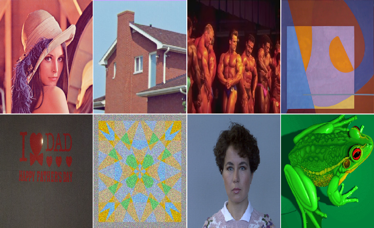
Figure 1: The test images. From left to right and top to bottom: Lena, House, Men, T1, T2, T3, Cara and Frog.

A growing number of research [21]-[24] indicates that quaternions are well adapted to color image processing by encoding color channels into three imaginary parts. The quaternion analytic signals are the boundary values of the functions in quaternion Hardy space [25]. Based on the quaternion analytic signal, researchers in [26] proposed some phase-based algorithms to detect the edge map of gray-scale images. It is shown that the introducing of quaternion analytic signal can reduce the influence of noise on edge detection results. It should be noted that although the tool of quaternion was applied, the algorithms (QDPC and QDPA) in [26] only considered the gray-scale images. Based on the quaternion Hardy filter and the improved Di Zenzo gradient operator, we propose a novel edge detection algorithm, which can be applied to color image.

The contributions of this paper are summarized as follows.

1. We propose a novel filter, named quaternion Hardy filter (QHF), for color image processing. Compared with quaternion analytic signal, our method has a better performance due to the flexible parameter selection of QHF.

2. Based on the QHF and the improved Di Zenzo gradient operator, we propose a robust color edge detection algorithm. It can enhance the color edge in a holistic manner by extracting the main features of the color image.

3. We set up a series of experiments to verify the denoising performance of the proposed algorithm in various environments. Visual and quantitative analysis are both conducted. Three widely used edge detection algorithms, Canny, Sobel and Prewitt, and two recent edge detection algorithms, QDPC, QDPA, DPC and MDPC, are compared with the proposed algorithm. In terms of peak SNR (PSNR) and similarity index measure (SSIM), the proposed algorithm presents the superiority in edge detection.

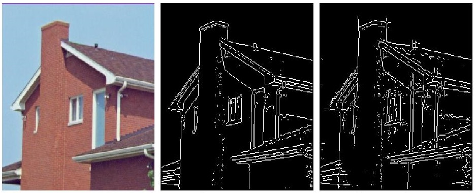
Figure 2: The noiseless House image (left). The edge maps obtained by IDZ gradient algorithm (middle) and the proposed algorithm (right).

The rest of the paper is organized as follows. Section II recalls some preliminaries of the improved Di Zenzo gradient operator, quaternions, quaternion Fourier transform, quaternion Hardy space and quaternion analytic signal. Section III presents the main result of the paper, it defines the novel algorithm for color-based edge detection of real-world images. Experimental results of the proposed algorithm are shown in Section IV. Conclusions and discussions of the future work are drawn in Section V.

II Preliminaries

This part recalls some preparatory knowledge of the improved Di Zenzo gradient operator [20], quaternions, quaternion Fourier transform [27], quaternion Hardy space [26] and quaternion analytic signal [28] which will be used throughout the paper.

II-A The improved Di Zenzo gradient operator

In the following, we recall the improved Di Zenzo gradient operator, namely the IDZ gradient operator, which will be combined with the quaternion Hardy filter to establish the novel edge detection algorithm in the next section.

Let $f$ be an $M\times{N}$ color image that maps a point $(x_{1},x_{2})$ to a vector $(f_{1}(x_{1},x_{2}),f_{2}(x_{1},x_{2}),f_{3}(x_{1},x_{2}))$. Then the square of the variation of $f$ at the position $(x_{1},x_{2})$ with the distance $\gamma$ in the direction $\theta$ is given by

$$\begin{aligned} df^{2}&:=\|f(x_{1}+\gamma{\cos\theta,x_{2}+\gamma{\sin\theta})-f(x_{1},x_{2})}\|_{2}^{2}\\ &\approx\sum\limits_{i=1}^{3}\left(\frac{\partial{f_{i}}}{\partial{x_{1}}}\gamma\cos\theta+\frac{\partial{f_{i}}}{\partial{x_{2}}}\gamma\sin\theta\right)^{2}\\ &=\gamma^{2}f(\theta),\end{aligned}$$ (1)

where

$$\begin{aligned} f(\theta):=&2\sum\limits_{i=1}^{3}\frac{\partial{f_{i}}}{\partial{x_{1}}}\frac{\partial{f_{i}}}{\partial{x_{2}}}\cos\theta\sin\theta\\ &+\sum\limits_{i=1}^{3}\left(\frac{\partial{f_{i}}}{\partial{x_{1}}}\right)^{2}\cos^{2}\theta+\sum\limits_{i=1}^{3}\left(\frac{\partial{f_{i}}}{\partial{x_{2}}}\right)^{2}\sin^{2}\theta.\end{aligned}$$ (2)

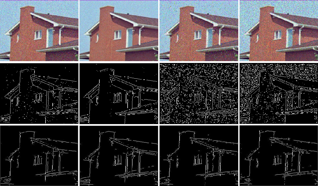
Figure 3: The first row is the noisy House image with additive Gaussian noise, Poisson noise, Salt & Pepper noise and Speckle noise from left to right. The second and third rows are the edge maps which are captured by IDZ algorithm and the proposed algorithm, respectively.

Let

$$\left\{\begin{aligned} &A:=\sum\limits_{i=1}^{3}\left(\frac{\partial{f_{i}}}{\partial{x_{1}}}\right)^{2};\\ &B:=\sum\limits_{i=1}^{3}\left(\frac{\partial{f_{i}}}{\partial{x_{2}}}\right)^{2};\\ &C:=\sum\limits_{i=1}^{3}\frac{\partial{f_{i}}}{\partial{x_{1}}}\frac{\partial{f_{i}}}{\partial{x_{2}}}.\end{aligned}\right.$$ (3)

Then the gradient magnitude $f_{\max}$ of the improved Di Zenzo’s gradient operator is given by

$$\begin{aligned} f_{\max}(\theta_{\max}):&=\max_{0\leq\theta\leq 2\pi}{f(\theta)}\\ =&\frac{1}{2}\bigg{(}A+C+\sqrt{(A-C)^{2}+(2B)^{2}}\bigg{)}.\end{aligned}$$ (4)

The gradient direction is defined as the value $\theta_{\max}$ that maximizes $f(\theta)$ over $0\leq\theta\leq 2\pi$

$$\theta_{\max}:= \mbox{sgn}(B)\arcsin\bigg{(}\frac{f_{\max}-A}{2f_{\max}-A-C}\bigg{)},$$ (5)

where $(A-C)^{2}+B^{2}\neq 0$, $\mbox{sgn}(B)=\left\{\begin{array}[]{ll}1,&{B\geq 0;}\\ -1,&{B<0.}\end{array}\right.$ When $(A-C)^{2}+B^{2}=0$, $\theta_{\max}$ is undefined.

It is important to note that the IDZ edge detector is designed to process real domain signals and don’t possess the capability of de-noising.

II-B Quaternions

As a natural extension of the complex space $\mathbb{C}$, the quaternion space $\mathbb{H}$ was first proposed by Hamilton in 1843 [29]. A complex number consists of two components: one real part and one imaginary part. While a quaternion $q\in\mathbb{H}$ has four components, i.e., one real part and three imaginary parts

$$q=q_{0}+q_{1}\mathbf{i}+q_{2}\mathbf{j}+q_{3}\mathbf{k},$$ (6)

where $q_{n}\in\mathbb{R},n=0,1,2,3$, and the basis elements $\{\mathbf{i},\mathbf{j},\mathbf{k}\}$ obey the Hamilton’s multiplication rules

$$\begin{aligned} \mathbf{i}^{2}&=\mathbf{j}^{2}=\mathbf{k}^{2}=\mathbf{i}\mathbf{j}\mathbf{k}=-1;\\ \mathbf{i}\mathbf{j}&=\mathbf{k},\mathbf{j}\mathbf{k}=\mathbf{i},\mathbf{k}\mathbf{i}=\mathbf{j};\\ \mathbf{j}\mathbf{i}&=-\mathbf{k},\mathbf{k}\mathbf{j}=-\mathbf{i},\mathbf{i}\mathbf{k}=-\mathbf{j}.\\ \end{aligned}$$ (7)

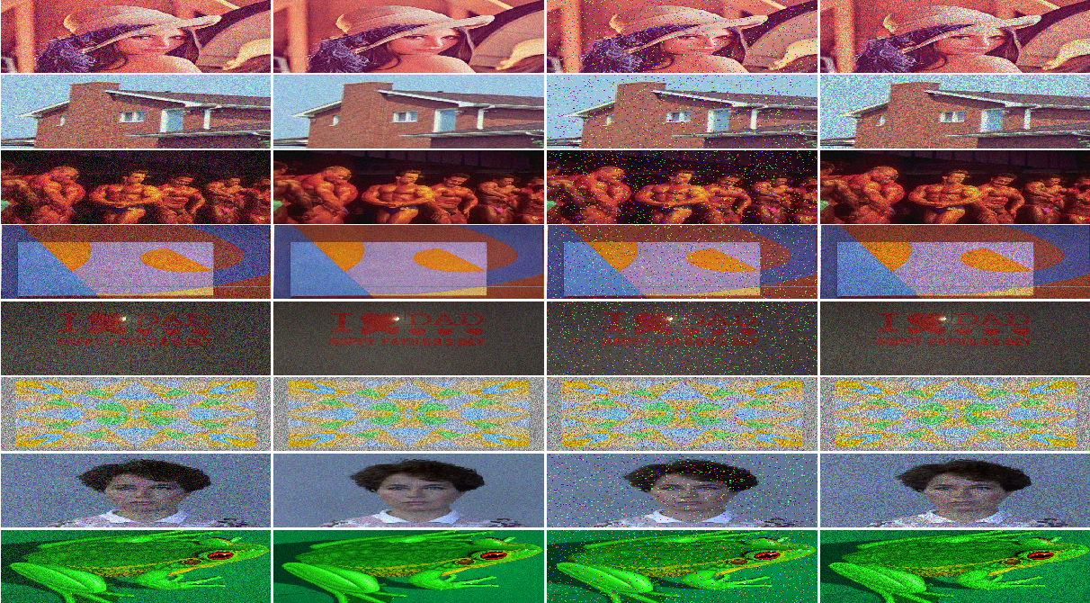
Figure 4: Noisy images. From left to right, they are obtained by adding: Gaussian noise, Poisson noise, Salt & Pepper noise and Speckle noise to the original images (Fig. 1).

Given a quaternion $q=q_{0}+q_{1}\mathbf{i}+q_{2}\mathbf{j}+q_{3}\mathbf{k}$, its quaternion conjugate is $\overline{q}:=q_{0}-q_{1}\mathbf{i}-q_{2}\mathbf{j}-q_{3}\mathbf{k}$. We write $\mathbf{Sc}(q):=\frac{1}{2}(q+\overline{q})=q_{0}$ and $\mathbf{Vec}(q):=\frac{1}{2}(q-\overline{q})=q_{1}\mathbf{i}+q_{2}\mathbf{j}+q_{3}\mathbf{k}$, which are the scalar and vector parts of $q$ , respectively. This leads to a modulus of $q\in\mathbb{H}$ defined by

$$|q|:=\sqrt{q\overline{q}}=\sqrt{\overline{q}q}=\sqrt{q_{0}^{2}+q_{1}^{2}+q_{2}^{2}+q_{3}^{2}},$$ (8)

where $q_{n}\in\mathbb{R},n=0,1,2,3$.

By (6), an $\mathbb{H}$-valued function $f:\mathbb{R}^{2}\rightarrow\mathbb{H}$ can be expressed as

$$\begin{aligned} f(x_{1},x_{2})=&f_{0}(x_{1},x_{2})+f_{1}(x_{1},x_{2})\mathbf{i}+f_{2}(x_{1},x_{2})\mathbf{j}\\ &+f_{3}(x_{1},x_{2})\mathbf{k},\end{aligned}$$ (9)

where $f_{n}:\mathbb{R}^{2}\rightarrow\mathbb{R}(n=0,1,2,3)$.

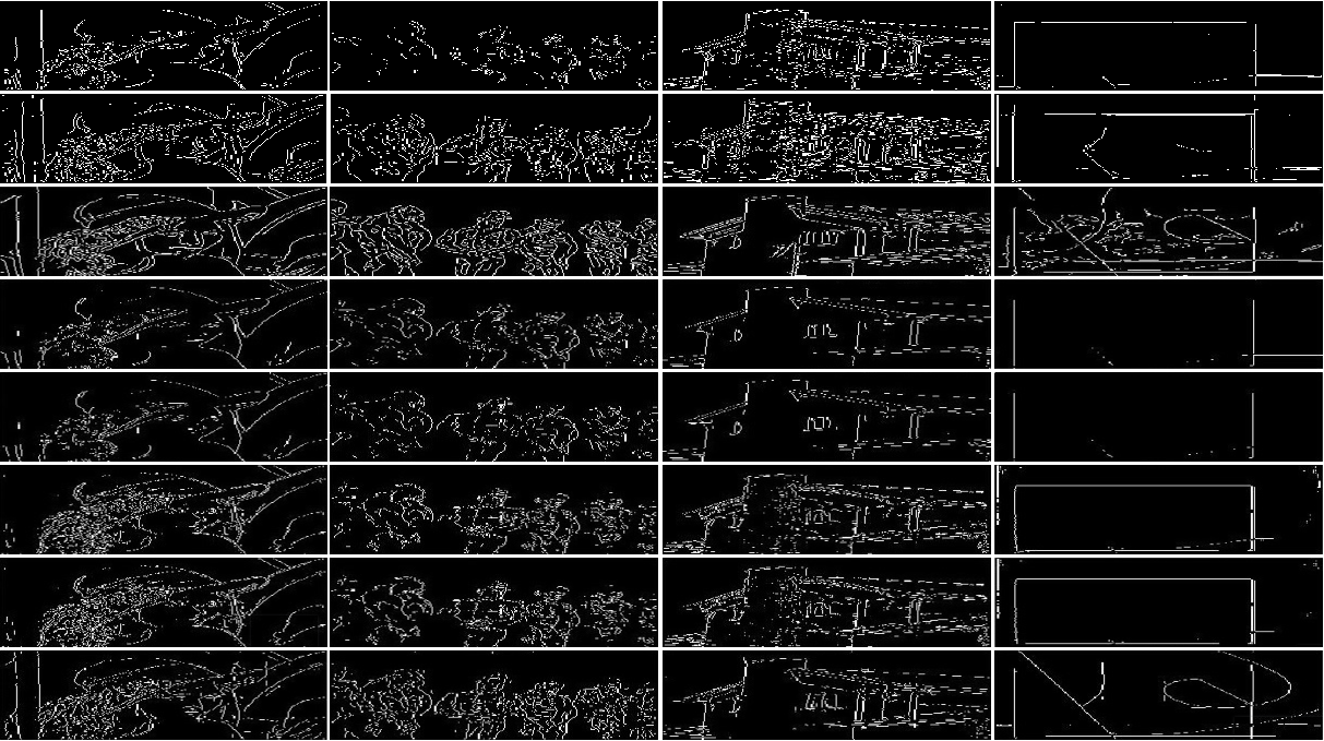
Figure 5: Edge maps of noiseless image Lena, Men , House and T1 generated by different edge detectors. From top to bottom: QDPC, QDPA, Canny, Sobel, Prewitt, DPC, MDPC and the proposed algorithm.

II-C Quaternion Fourier transform

Suppose that $f$ is an absolutely integrable complex function defined on $\mathbb{R}$, then the Fourier transform [30] of $f$ is given by

$$\widehat{f}(w):=\frac{1}{\sqrt{2\pi}}\int_{\mathbb{R}}f(x)e^{-iwx}d{x},$$ (10)

where $w$ denotes the angular frequency. Moreover, if $\widehat{f}$ is an absolutely integrable complex function defined on $\mathbb{R}$ , then $f$ can be reconstructed by the Fourier transform of $f$ and is expressed by

$$f(x)=\frac{1}{\sqrt{2\pi}}\int_{\mathbb{R}}\widehat{f}(w)e^{iwx}dw.$$ (11)

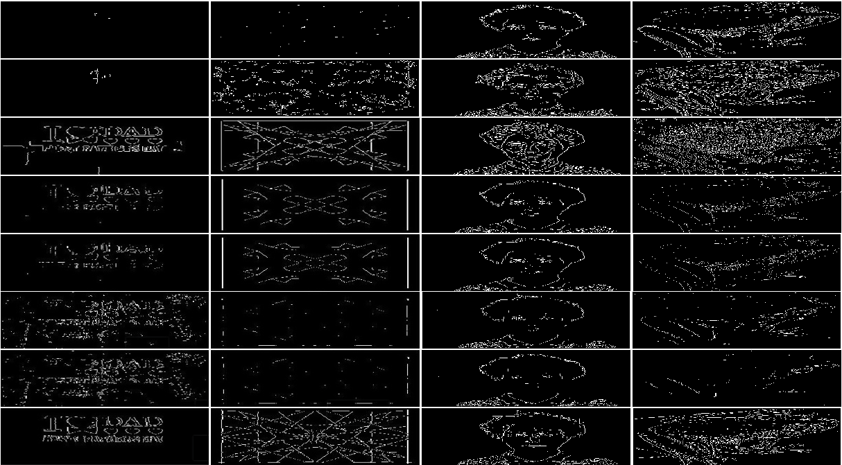
Figure 6: Edge maps of noiseless image T2, T3, Cara and Frog generated by different edge detectors. From top to bottom: QDPC, QDPA, Canny, Sobel, Prewitt, DPC, MDPC and the proposed algorithm.

The quaternion Fourier transform, regarded as an extension of Fourier transform in quaternion domain, plays a vital role in grayscale image processing. The first definition of the quaternion Fourier transform was given in 1992 [31] and the first application to color images was discussed in 1996 [32]. It was recently applied to find the envelope of the image [33]. The application of quaternion Fourier transform on color images was discussed in [24], [34]. The Plancherel and inversion theorems of quaternion Fourier transform in the square integrable signals class was established in [35]. Due to the non-commutativity of the quaternions, there are various types of quaternion Fourier transforms. In the following, we focus our attention on the two-sided quaternion Fourier transform (QFT).

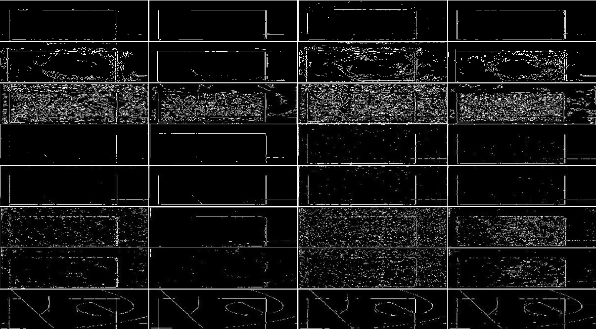
Figure 7: The edge maps of the noisy image T1 given by different algorithms. From top to bottom: QDPC, QDPA, Canny, Sobel, Prewitt, DPC, MDPC and the proposed algorithm. The first column to the last column show respectively the edge maps of T1 with Gaussian noise, Poisson noise, Salt & Pepper noise and Speckle noise.

Suppose that $f$ is an absolutely integrable $\mathbb{H}$-valued function defined on $\mathbb{R}^{2}$, then the continuous quaternion Fourier transform of $f$ is defined by

$$(\mathcal{F}f)(w_{1},w_{2}):=\frac{1}{2\pi}\int_{\mathbb{R}^{2}}e^{-\mathbf{i}w_{1}x_{1}}f(x_{1},x_{2})e^{-\mathbf{j}w_{2}x_{2}}d{x_{1}}d{x_{2}},$$ (12)

where $w_{l}$ and $x_{l}$ denote the 2D angular frequency and 2D space ($l=1,2$), respectively.

Furthermore, if $f$ is an absolutely integrable $\mathbb{H}$-valued function defined on $\mathbb{R}^{2}$, then the continuous inverse quaternion Fourier transform (IQFT) of $f$ is defined by

$$({\mathcal{F}}^{-1}f)(x_{1},x_{2}):=\frac{1}{2\pi}\int_{\mathbb{R}^{2}}e^{\mathbf{i}w_{1}x_{1}}f(w_{1},w_{2})e^{\mathbf{j}w_{2}x_{2}}d{w_{1}}d{w_{2}},$$ (13)

where $w_{l}$ and $x_{l}$ denote the 2D angular frequency and 2D space ($l=1,2$), respectively.

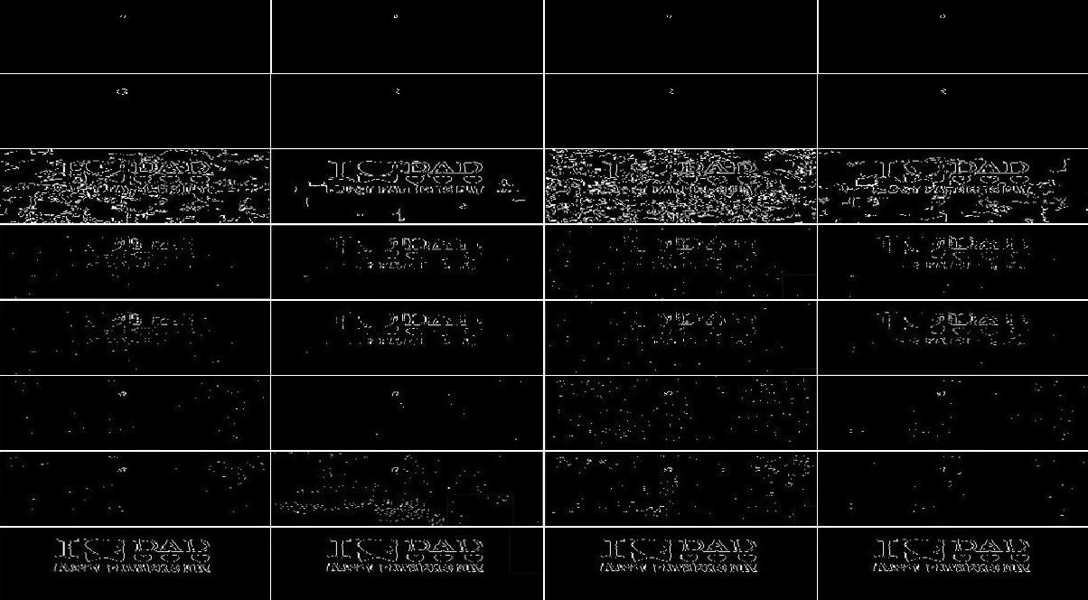
Figure 8: The edge maps of the noisy image T2 given by different algorithms. From top to bottom: QDPC, QDPA, Canny, Sobel, Prewitt, DPC, MDPC and the proposed algorithm. The first column to the last column show respectively the edge maps of T2 with Gaussian noise, Poisson noise, Salt & Pepper noise and Speckle noise.

The discrete quaternion Fourier transform (DQFT) and its inverse is introduced by Sangwine [36] in 1996. Suppose that the discrete array $f(m,n)$ is of dimension $M\times N$. The DQFT has the following form

$$\mathcal{F}_{D}[f](p,s):=\frac{1}{\sqrt{MN}}{\sum_{m=0}^{M-1}}{\sum_{n=0}^{N-1}}e^{-\mathbf{i}2\pi\frac{mp}{M}}f(m,n)e^{-\mathbf{j}2\pi\frac{ns}{N}}.$$ (14)

And the inverse discrete quaternion Fourier transform (IDQFT) is

$$f(m,n):=\frac{1}{\sqrt{MN}}{\sum_{p=0}^{M-1}}{\sum_{s=0}^{N-1}}e^{\mathbf{i}2\pi\frac{mp}{M}}\mathcal{F}_{D}[f](p,s)e^{\mathbf{j}2\pi\frac{ns}{N}}.$$ (15)

II-D Quaternion Hardy space

Let ${\mathbb{C}}:=\{z|z=x+si,x,s\in\mathbb{R}\}$ be the complex plane and a subset of ${\mathbb{C}}$ is defined by ${\mathbb{C}}^{+}:=\{z|z=x+si,x,s\in\mathbb{R},s>0\}$, namely upper half complex plane.

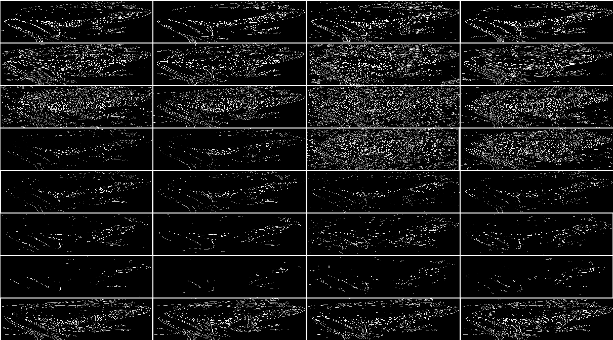
Figure 9: The edge maps of the noisy image Frog given by different algorithms. From top to bottom: QDPC, QDPA, Canny, Sobel, Prewitt, DPC, MDPC and the proposed algorithm. The first column to the last column show respectively the edge maps of Frog with Gaussian noise, Poisson noise, Salt & Pepper noise and Speckle noise.

The Hardy space ${\mathbf{H}}^{2}(\mathbb{C}^{+})$ on the upper half complex plane consists of functions $c$ satisfying the following conditions

$$\left\{\begin{aligned} &\frac{\partial}{\partial\overline{z}}c(z)=0;\\ &(\sup\limits_{s>0}\int_{\mathbb{R}}|c(x+si)|^{2}dx)^{\frac{1}{2}}<\infty.\end{aligned}\right.$$ (16)

The generalization [26] to higher dimension is given as follows. Let $\mathbb{C}_{\mathbf{i}\mathbf{j}}:=\{(z_{1},z_{2})|z_{1}=x_{1}+s_{1}\mathbf{i},z_{2}=x_{2}+s_{2}\mathbf{j},x_{l},s_{l}\in\mathbb{R},l=1,2\}$ and a subset of $\mathbb{C}_{\mathbf{i}\mathbf{j}}$ is defined by $\mathbb{C}_{\mathbf{i}\mathbf{j}}^{+}:=\{(z_{1},z_{2})|z_{1}=x_{1}+s_{1}\mathbf{i},z_{2}=x_{2}+s_{2}\mathbf{j},x_{l},s_{l}\in\mathbb{R},s_{l}>0,l=1,2\}.$ The quaternion Hardy space $\mathbf{Q}^{2}(\mathbb{C}_{\mathbf{i}\mathbf{j}}^{+})$ consists of all functions satisfying the following conditions

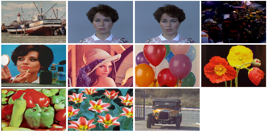
Figure 10: The test images. These images are randomly selected from the public image dataset (http://decsai.ugr.es/cvg/dbimagenes/).

$$\left\{\begin{aligned} &\frac{\partial}{\partial\overline{z_{1}}}h(z_{1},z_{2})=0;\\ &h(z_{1},z_{2})\frac{\partial}{\partial\overline{z_{2}}}=0;\\ &(\sup\limits_{\begin{subarray}{c}s_{1}>0\\ s_{2}>0\end{subarray}}\int_{\mathbb{R}^{2}}|h(x_{1}+s_{1}\mathbf{i},x_{2}+s_{2}\mathbf{j})|^{2}dx_{1}dx_{2})^{\frac{1}{2}}<\infty,\end{aligned}\right.$$ (17)

where $\frac{\partial}{\partial\overline{z_{1}}}:=\frac{\partial}{\partial{x_{1}}}+\mathbf{i}\frac{\partial}{\partial{s_{1}}}$, $\frac{\partial}{\partial\overline{z_{2}}}:=\frac{\partial}{\partial{x_{2}}}+\mathbf{j}\frac{\partial}{\partial{s_{2}}}$.

II-E Quaternion analytic signal

In the following, we review the concept of analytic signal. Given a real signal $f$, combined with its own Hilbert transform, then the analytic signal of $f$ is given by

$$f_{a}(x):=f(x)+i\mathcal{H}[f](x),x\in\mathbb{R},$$ (18)

where $\mathcal{H}[f]$ denotes the Hilbert transform of $f$ and is defined by

$$\mathcal{H}[f](x):=\frac{1}{\pi}\lim\limits_{\varepsilon\to 0^{+}}\int_{\varepsilon\leq|x-s|}\frac{f(s)}{x-s}ds.$$ (19)

The Fourier transform of an analytic $f_{a}$ defined in (18) is given by

$$\widehat{f_{a}}(w)=\left(1+\mbox{sgn}(w)\right)\widehat{f}(w),$$ (20)

where $w\in\mathbb{R}$.

A natural extension of the analytic signal from 1D to 4D space in the quaternion setting is called quaternion analytic signal. It was proposed by Bülow and Sommer [HypercomplexsignalsSommer] using partial and total Hilbert transform associated with QFT. Given a 2D quaternion valued signal $f$, combined with its own quaternion partial and total Hilbert transform, then we get a quaternion analytic signal $f_{q}$ [HypercomplexsignalsSommer] as follows

$$f_{q}(x_{1},x_{2}):= f(x_{1},x_{2})+\mathbf{i}\mathcal{H}_{x_{1}}[f](x_{1})$$ (21)

$$+\mathcal{H}_{x_{2}}[f](x_{2})\mathbf{j}+\mathbf{i}\mathcal{H}_{{x_{1}}{x_{2}}}[f](x_{1},x_{2})\mathbf{j},$$

where

$$\begin{aligned} &\mathcal{H}_{x_{1}}[f](x_{1}):=\frac{1}{\pi}\lim\int\frac{f(t_{1},x_{2})}{x_{1}-t_{1}}dt_{1},\\ &\mathcal{H}_{x_{2}}[f](x_{2}):=\frac{1}{\pi}\lim\int\frac{f(x_{1},t_{1})}{x_{2}-t_{1}}dt_{1},\\ \end{aligned}$$ (22)

are the quaternion partial Hilbert transform of $f$ along the $x_{1}$-axis, $x_{2}$-axis, respectively. While

$$\mathcal{H}_{{x_{1}}{x_{2}}}[f](x_{1},x_{2}):=\frac{1}{\pi}\lim\int\frac{f(t_{1},t_{2})}{(x_{1}-t_{1})(x_{2}-t_{2})}dt_{1}dt_{2},$$ (23)

is the quaternion total Hilbert transform along the $x_{1}$ and $x_{2}$ axes. By direct computation, the quaternion Fourier transform of quaternion analytic signal is given by

$$(\mathcal{F}{f_{q}})(w_{1},w_{2})= [1+\mbox{sgn}(w_{1})][1+\mbox{sgn}(w_{2})]$$ (24)

$$(\mathcal{F}{f})(w_{1},w_{2}).$$

III Proposed algorithm

In this section, we introduce our new color edge detection algorithm. To begin with, the definition of quaternion Hardy filter is presented.

III-A Quaternion Hardy filter

The quaternion analytic signal $f_{q}$ can be regarded as the output signal of a filter with input $f$. The system function of this filter is

$$H_{1}(w_{1},w_{2}):=[1+\mbox{sgn}(w_{1})][1+\mbox{sgn}(w_{2})].$$ (25)

In this paper, we use a novel filter, named quaternion Hardy filter (QHF), to construct a high-dimensional analytic signal. The system function of QHF is defined by

$$H(w_{1},w_{2},s_{1},s_{2}):= [1+\mbox{sgn}(w_{1})][1+\mbox{sgn}(w_{2})]$$ (26)

$$e^{-\mid{w_{1}}\mid{s_{1}}}e^{-\mid{w_{2}}\mid{s_{2}}},$$

where $s_{1}\geq 0,s_{2}\geq 0$ are parameters of the system function. The factors $(1+\mbox{sgn}(w_{1}))(1+\mbox{sgn}(w_{2}))$ and $e^{-\mid{w_{1}}\mid{s_{1}}}e^{-\mid{w_{2}}\mid{s_{2}}}$ play different roles in quaternion Hardy filter. The former performs Hilbert transform on the input signal, while the later plays a role of suppressing the high-frequency. On the one hand, the Hilbert transform operation can selectively emphasize the edge feature of an input object. On the other hand, the low-pass filtering can improve the ability of noise immunity for the QHF. It can be seen that as increase with $s_{1},s_{2}$, the effect of inhibiting for the high frequency becomes more obvious. In particular, if $s_{1}=s_{2}=0$, then $e^{-\mid{w_{1}}\mid{s_{1}}}e^{-\mid{w_{2}}\mid{s_{2}}}=1$, it follows that

$$H(w_{1},w_{2},0,0)=H_{1}(w_{1},w_{2}),$$ (27)

which means that there is no effect in high frequency inhibiting.

Parameters $s_{1}$ and $s_{2}$ play the role of low-pass filtering in vertical and horizontal directions, respectively. When the signal frequencies in the two directions are similar, then $s_{1}$ and $s_{2}$ can be set to the same value. If the signal frequencies in these two directions are different, then $s_{1}$ and $s_{2}$ should be different. For example, if the horizontal noise in the image is large, the value of $s_{2}$ should be set larger to enhance the anti-noise ability in that direction. This means that the QHF is very general and flexible, and it can solve many problems that can’t be solved well by quaternion analytic signal.

TABLE I: The PSNR comparison values of Lena, Men, House and T1. Types of noise: I- Gaussian noise, II- Poisson noise, III- Salt & Pepper noise and IV- Speckle noise.

		QDPC	QDPA	Canny	Sobel	Prewitt	MDPC	DPC	IDZ	Ours
LENA	I	58.1631	56.8276	56.6985	64.7819	64.6047	57.6375	57.6707	53.9715	64.8622
	II	58.1378	56.9719	57.5531	68.2679	68.1332	59.9609	60.0363	56.0557	65.8570
	III	58.1625	56.8949	55.8291	62.4449	62.6426	57.7647	57.6952	54.2721	63.0016
	IV	58.1266	58.8760	56.4122	64.4007	64.3951	58.8433	58.7682	53.8232	64.6239
MEN	I	58.8880	57.3084	59.1716	62.7258	62.7488	58.7690	58.8037	53.7155	62.9965
	II	58.8770	57.4573	63.4944	66.3657	66.2739	60.9465	61.0934	59.2063	65.2541
	III	58.8746	57.1006	57.3177	58.9356	59.2481	58.2379	58.2515	54.4117	62.0697
	IV	58.8770	57.4397	60.6136	62.9773	62.9611	60.3605	60.4286	56.3922	63.0900
HOUSE	I	59.1106	56.6819	56.3984	64.9506	65.1998	57.7217	57.7132	54.0252	61.4998
	II	59.1389	56.9562	63.4558	67.6564	67.9324	60.0384	60.1424	56.0046	63.4681
	III	59.0990	56.5921	56.7973	62.9551	63.1633	58.0498	57.9419	54.3644	61.0881
	IV	59.0520	56.2835	56.0536	63.8801	64.0296	58.2135	58.0122	53.7992	61.0322
Image T1	I	64.9126	62.7373	54.6441	71.3263	72.8126	64.3338	61.0803	53.9459	69.7830
	II	65.2066	62.2319	57.7629	78.5871	77.5450	68.2203	69.1860	57.4738	74.1626
	III	65.2066	62.7854	54.8312	67.8883	68.4996	59.1397	57.6659	54.3844	68.8984
	IV	65.0181	62.4863	55.7384	71.3680	72.0796	62.1912	59.4687	53.8051	70.2784

TABLE II: The PSNR comparison values of T2, T3, Cara and Frog. Types of noise: I- Gaussian noise, II- Poisson noise, III- Salt & Pepper noise and IV- Speckle noise.

		QDPC	QDPA	Canny	Sobel	Prewitt	DPC	MDPC	Ours
Image T2	I	82.3162	76.5637	57.9033	67.5161	62.0191	61.7502	61.6269	67.7956
	II	82.1459	79.1356	66.8262	70.8302	63.8282	61.8739	60.8068	70.8856
	III	77.6624	70.3738	55.8679	66.7100	60.4750	61.2672	61.0374	66.8058
	IV	82.3162	75.1562	61.7685	68.6092	61.7823	61.8209	61.7823	68.7155
Image T3	I	75.3200	59.8140	53.3384	61.5886	61.6987	62.8951	62.9903	62.9955
	II	75.3265	60.648	54.0415	62.2696	62.2132	66.3745	66.1757	64.3923
	III	74.4772	59.1910	53.7885	58.5834	58.4737	63.8012	63.8826	61.8965
	IV	74.7422	58.5271	53.0448	61.7655	61.8349	62.0452	61.8975	63.0900
Image Cara	I	62.4899	59.2739	55.6093	64.7180	64.7514	64.1129	62.9773	65.9913
	II	63.0755	61.1621	60.2663	66.1169	66.3480	64.3532	63.4694	66.7686
	III	60.7350	57.7018	55.2998	55.0236	63.4468	63.3421	61.7183	63.4500
	IV	62.4128	59.9237	55.4111	55.4800	64.7758	64.0322	62.9250	64.8002
Image Frog	I	59.5452	57.6452	57.9129	63.3546	64.3588	60.8068	59.8769	64.3217
	II	60.0641	59.0153	61.1945	65.5119	65.5584	60.8961	60.2096	65.8411
	III	58.6196	56.5482	56.3742	56.3881	63.3670	60.3883	59.1801	63.8809
	IV	59.2447	57.5758	57.8310	57.2878	64.0090	60.6560	59.6291	63.9898

For any fixed $s_{1},s_{2}\geq 0$, denote by $f_{H}(x_{1},x_{2},s_{1},s_{2})$ the output signal of the QHF with input $f(x_{1},x_{2})$. By the definition, we have

$$(\mathcal{F}{f_{H}})(w_{1},w_{2},s_{1},s_{2})=[1+\mbox{sgn}(w_{1})][1+\mbox{sgn}(w_{2})]$$ (28)

$$e^{-\mid{w_{1}}\mid{s_{1}}}e^{-\mid{t_{2}}\mid{s_{2}}}(\mathcal{F}{f})(w_{1},w_{2}).$$

Here, the QFT acts on the variable $x_{1},x_{2}$. We will show that as a function of $z_{1}=x_{1}+\mathbf{i}s_{1}$ and $z_{2}=x_{2}+\mathbf{j}s_{2}$, $f_{H}$ belongs to the quaternion Hardy space $\mathbf{Q}^{2}(\mathbb{C}_{\mathbf{i}\mathbf{j}}^{+})$.

Theorem 1

Let $f\in L^{2}(\mathbb{R}^{2},\mathbb{H})$ and $f_{H}$ be given above. Then $f_{H}\in\mathbf{Q}^{2}(\mathbb{C}_{\mathbf{i}\mathbf{j}}^{+})$ .

Proof III.1

Using inverse quaternion Fourier transform defined by Eq. (13), we have that

$$f_{H}(x_{1},x_{2},s_{1},s_{2})= \frac{1}{2\pi}\int_{\mathbb{R}^{2}}e^{\mathbf{i}w_{1}x_{1}}[1+\mbox{sgn}(w_{1})]$$ (29)

$$[1+\mbox{sgn}(w_{2})]e^{-\mid{w_{1}}\mid{s_{1}}}e^{-\mid{w_{2}}\mid{s_{2}}}$$

$$(\mathcal{F}{f})(w_{1},w_{2})e^{\mathbf{j}w_{2}x_{2}}d{w_{1}}d{w_{2}}.$$

Taking the derivative of $f_{H}$ with respect to $\overline{z_{1}}$, we get

$$\frac{\partial}{\partial\overline{z_{1}}}f_{H}(x_{1},x_{2},s_{1},s_{2})$$ (30)

$$= [\frac{\partial}{\partial{x_{1}}}+\mathbf{i}\frac{\partial}{\partial{s_{1}}}]f_{H}(x_{1},x_{2},s_{1},s_{2})$$

$$= \frac{1}{2\pi}\int_{\mathbb{R}^{2}}\mathbf{i}(w_{1}-|w_{1}|)e^{\mathbf{i}w_{1}x_{1}}[1+\mbox{sgn}(w_{1})][1+\mbox{sgn}(w_{2})]$$

$$e^{-\mid{w_{1}}\mid{s_{1}}}e^{-\mid{w_{2}}\mid{s_{2}}}(\mathcal{F}{f})(w_{1},w_{2})e^{\mathbf{j}w_{2}x_{2}}d{w_{1}}d{w_{2}}$$

$$= 0.$$

The last equality holds since the integrand vanishes identically. Similarly,

$$f_{H}(x_{1},x_{2},s_{1},s_{2})\frac{\partial}{\partial\overline{z_{2}}}$$ (31)

$$= \frac{\partial}{\partial{x_{2}}}f_{H}(x_{1},x_{2},s_{1},s_{2})+\frac{\partial}{\partial{s_{2}}}f_{H}(x_{1},x_{2},s_{1},s_{2})\mathbf{j}$$

$$= \frac{1}{2\pi}\int_{\mathbb{R}^{2}}e^{\mathbf{i}w_{1}x_{1}}[1+\mbox{sgn}(w_{1})][1+\mbox{sgn}(w_{2})]$$

$$e^{-\mid{w_{1}}\mid{s_{1}}}e^{-\mid{w_{2}}\mid{s_{2}}}(\mathcal{F}{f})(w_{1},w_{2})\mathbf{j}(w_{2}-|w_{2}|)e^{\mathbf{j}w_{2}x_{2}}d{w_{1}}d{w_{2}}$$

$$= 0.$$

For any fixed $s_{1}>0,s_{2}>0$, from (28) we can obtain that

$$(\mathcal{F}{f_{H}})(w_{1},w_{2},s_{1},s_{2})\leq 4(\mathcal{F}{f})(w_{1},w_{2}).$$ (32)

According to the QFT Parseval’s identity [ChengQFT], we obtain that

$$\int_{\mathbb{R}^{2}}|(\mathcal{F}{f_{H}})(w_{1},w_{2},s_{1},s_{2})|^{2}dw_{1}dw_{2}$$ (33)

$$= \int_{\mathbb{R}^{2}}|f_{H}(x_{1},x_{2},s_{1},s_{2})|^{2}dx_{1}dx_{2},$$

$$\int_{\mathbb{R}^{2}}|(\mathcal{F}{f})(w_{1},w_{2})|^{2}dw_{1}dw_{2}$$ (34)

$$= \int_{\mathbb{R}^{2}}|f(x_{1},x_{2})|^{2}dx_{1}dx_{2}.$$

Using (32), (33) and (34), a direct computation shows that

$$\sup\limits_{\begin{subarray}{c}s_{1}>0\\ s_{2}>0\end{subarray}}\int_{\mathbb{R}^{2}}|f_{H}(x_{1}+s_{1}\mathbf{i},x_{2}+s_{2}\mathbf{j})|^{2}dx_{1}dx_{2}$$ (35)

$$\leq\sup\limits_{\begin{subarray}{c}s_{1}>0\\ s_{2}>0\end{subarray}}16\int_{\mathbb{R}^{2}}|(\mathcal{F}{f})(w_{1},w_{2})|^{2}dw_{1}dw_{2}<\infty.$$

The proof is complete.

III-B Color edge detection algorithm

In this section, the edge detector based on QHF are described. The IDZ approach for edge detection based on the QHF consists in using (14), (15) and (26) to obtain the high-dimensional analytic signal, and then use it as inputs for an appropriately defined robust edge detection algorithm. Let us now give the details of the quaternion Hardy filter based algorithm. They are divided by the following steps.

• Step 1. Given an input digital color image of size $M\times N$, associate it with a $\mathbb{H}$-valued signal

  $$f:=f_{1}\mathbf{i}+f_{2}\mathbf{j}+f_{3}\mathbf{k},$$ (36)

  where $f_{1},f_{2}$ and $f_{3}$ represent respectively the red, green and blue components of the given color image.

• Step 2. Compute the DQFT of the $f$ using equation (14). The result will be $\mathcal{F}_{D}[f]$.

• Step 3. For fixed $s_{1}>0,s_{2}>0$ (the values of parameters $s_{1}$ and $s_{2}$ of the original image ranged from 1.0 to 2.0, and those of the noisy image ranged from 1.0 to 8.0, for details please refer Table LABEL:tab1-parameter-LENA-LABEL:tab1-parameter-FROG), multiplying $\mathcal{F}_{D}[f]$ by the system function (26) of the QHF. Then we obtain the DQFT of $f_{H}$ which has the following form

  $$(\mathcal{F}_{D}{f_{H}})(w_{1},w_{2},s_{1},s_{2})=[1+\mbox{sgn}(w_{1})]$$ (37)

  $$[1+\mbox{sgn}(w_{2})]e^{-\mid{w_{1}}\mid{s_{1}}}e^{-\mid{t_{2}}\mid{s_{2}}}(\mathcal{F}_{D}{f})(w_{1},w_{2}).$$

  This is the most significant step in our algorithm, because it allows the advantages of QHF to be presented.

• Step 4. Compute the inverse DQFT for $\mathcal{F}_{D}[f_{H}]$ by applying equation (15), we obtain $f_{H}$.

• Step 5. Extract the vector part of $f_{H}$, we obtain

  $$\mathbf{Vec}(f_{H})=h_{1}\mathbf{i}+h_{2}\mathbf{j}+h_{3}\mathbf{k},$$ (38)

  where $h_{k}$, $k=1,2,3$ are real-valued functions. In the following, we will operate IDZ algorithm based on $\mathbf{Vec}(f_{H})$ instead of $f$.

• Step 6. Perform the IDZ gradient operator to $\mathbf{Vec}(f_{H})$. Applying equation (3), we obtain

  $$\left\{\begin{aligned} &A=\sum\limits_{k=1}^{3}(\frac{\partial{h_{k}}}{\partial{x_{1}}})^{2};\\ &B=\sum\limits_{k=1}^{3}(\frac{\partial{h_{k}}}{\partial{x_{2}}})^{2};\\ &C=\sum\limits_{k=1}^{3}\frac{\partial{h_{k}}}{\partial{x_{1}}}\frac{\partial{h_{k}}}{\partial{x_{2}}},\end{aligned}\right.$$ (39)

  then we substitute them into equation (4), obtain

  $$\mathbf{Vec}(f_{H})_{\max}=\frac{1}{2}\bigg{(}A+C+\sqrt{(A-C)^{2}+(2B)^{2}}\bigg{)}.$$ (40)

• Step 7. Finally, we obtain the processed result, edge map, by applying the nonmaxmum suppress.

IV Experimental results

In this section, we shall demonstrate the effectiveness of the proposed algorithm for color image edge detection.

Here both visual and quantitative analysis for edge detection are considered in our experiments. All experiments are programmed in Matlab R2016b. To validate the effectiveness of the proposed method, we have carried out verification on many images, eight of which are shown in Fig. 1. The images are from the public image dataset (http://decsai.ugr.es/cvg/dbimagenes/), which has been used by previous researchers. It consists of 805 test images with 3 different size scales. There are 3 and 6 classes in color images and gray images, respectively. Here, the Gaussian filter [37, 38] is applied to these algorithms (Canny, Sobel, Prewitt, DPC and MDPC), since they doesn’t have the ability of resisting noise. Digital images distorted with different types of noise such as I- Gaussian noise [39], II- Poisson noise, III- Salt & Pepper noise and IV- Speckle noise. The ideal noiseless (Fig. 1) and noisy images (Fig. 4) are both taken into account.

TABLE III: The SSIM comparison values of Lena, Men, House and T1. Types of noise: I- Gaussian noise, II- Poisson noise, III- Salt & Pepper noise and IV- Speckle noise.

		QDPC	QDPA	Canny	Sobel	Prewitt	DPC	MDPC	Ours
LENA	I	0.4346	0.3473	0.6568	0.8041	0.8011	0.2876	0.2986	0.8058
	II	0.4365	0.3641	0.8593	0.9165	0.9124	0.6198	0.6200	0.9275
	III	0.4331	0.3632	0.5299	0.5406	0.5611	0.1711	0.1710	0.7155
	IV	0.4301	0.3579	0.5658	0.7604	0.7613	0.4953	0.4959	0.7872
MEN	I	0.4736	0.3644	0.6850	0.6673	0.6722	0.4342	0.4343	0.6878
	II	0.4723	0.3741	0.8739	0.8575	0.8572	0.6523	0.6522	0.8843
	III	0.4629	0.3379	0.3973	0.1668	0.1726	0.1375	0.1376	0.4669
	IV	0.4730	0.3744	0.7670	0.7200	0.7281	0.5633	0.5677	0.7463
HOUSE	I	0.5728	0.6699	0.4250	0.8475	0.8522	0.2289	0.2292	0.8518
	II	0.6015	0.7218	0.8503	0.9183	0.9134	0.5101	0.5106	0.9192
	III	0.3814	0.5899	0.3759	0.5767	0.5921	0.1419	0.1423	0.6723
	IV	0.4343	0.6188	0.3387	0.7502	0.7756	0.2691	0.2672	0.6707
Image T1	I	0.8417	0.7673	0.1449	0.9562	0.9309	0.3935	0.7128	0.9196
	II	0.8441	0.7674	0.4470	0.9270	0.9456	0.9191	0.8435	0.9652
	III	0.8440	0.7617	0.1227	0.7497	0.8045	0.0637	0.1679	0.8833
	IV	0.8454	0.7578	0.3621	0.8970	0.9121	0.4338	0.6074	0.9139

TABLE IV: The SSIM comparison values for T2, T3, Cara and Frog. Types of noise: I- Gaussian noise, II- Poisson noise, III- Salt & Pepper noise and IV- Speckle noise.

		QDPC	QDPA	Canny	Sobel	Prewitt	DPC	MDPC	Ours
Image T2	I	0.9957	0.9815	0.4350	0.8217	0.8314	0.3271	0.3204	0.9248
	II	0.9954	0.9926	0.9034	0.9202	0.9311	0.5865	0.5635	0.9664
	III	0.9674	0.9428	0.1942	0.7720	0.7880	0.3206	0.3153	0.9098
	IV	0.9957	0.9819	0.7197	0.8914	0.8901	0.3780	0.3584	0.9483
Image T3	I	0.9456	0.4588	0.0827	0.3983	0.4001	0.1116	0.0964	0.7560
	II	0.9469	0.5161	0.1872	0.6195	0.6175	0.3285	0.3330	0.8434
	III	0.9324	0.3999	0.0675	0.2326	0.2430	0.1729	0.1745	0.7192
	IV	0.9389	0.3382	0.0386	0.3714	0.3497	0.0803	0.0725	0.6850
Image Cara	I	0.7624	0.5932	0.1991	0.8394	0.8499	0.8041	0.7584	0.8500
	II	0.8024	0.7220	0.6606	0.8923	0.8907	0.8069	0.7953	0.8916
	III	0.4524	0.3382	0.1682	0.0828	0.7135	0.7463	0.6085	0.7302
	IV	0.7625	0.6328	0.2010	0.1433	0.8457	0.7993	0.7511	0.7998
Image Frog	I	0.6200	0.5090	0.5309	0.8025	0.8185	0.6271	0.5614	0.8220
	II	0.6490	0.6194	0.7770	0.8396	0.8510	0.6384	0.5960	0.8548
	III	0.4830	0.3636	0.3343	0.2443	0.7139	0.5718	0.4464	0.7231
	IV	0.6128	0.5276	0.5572	0.4034	0.7939	0.6116	0.5416	0.8003

IV-A Visual comparisons

In terms of visual analysis, a color-based method IDZ and seven widely used and noteworthy methods QDPC, QDPA, Canny, Sobel, Prewitt, Differential Phase Congruence (DPC) and Modified Differential Phase Congruence (MDPC) will be compared with our algorithm.

IV-A1 Color-based algorithm

In this part, we first compare the proposed algorithm with the IDZ gradient algorithm. In order to make the experiment more convincing, we used Gaussian filter before IDZ algorithm to achieve the effect of denoising. Fig. 2 presents the edge map of the noiseless House image, while Fig. 3 presents the edge map of the House image corrupted with four different types of noise. It can be seen from the second row of Fig. 3 that IDZ gradient algorithm performs well in the first two images of the first line, while poorly in the last two images. This illustrates that the IDZ gradient algorithm’s limitations as a edge detector. The third row of Fig. 3 shows the detection result of the proposed algorithm. It preserves details more clearly than the second row. It demonstrates that the proposed algorithm gives robust performance compared to that of the IDZ gradient algorithm.

IV-A2 Grayscale-based algorithms

TABLE V: The PSNR comparison values for Fig. 10. Types of noise: I- Gaussian noise, II- Poisson noise, III- Salt & Pepper noise and IV- Speckle noise.

	QDPC	QDPA	Canny	Sobel	Prewitt	DPC	MDPC	Ours
I	59.5875	57.1603	54.8202	61.4068	61.8794	58.5991	59.1803	62.5796
II	59.7487	58.0289	56.0615	61.7013	62.0238	59.1115	59.5553	64.3704
III	58.9160	56.4631	54.2282	59.9397	60.7958	57.5608	58.4340	61.6690
IV	59.4685	57.4581	54.7294	60.3342	61.5622	58.4213	59.1584	62.9552

TABLE VI: The SSIM comparison values for Fig. 10. Types of noise: I- Gaussian noise, II- Poisson noise, III- Salt & Pepper noise and IV- Speckle noise.

	QDPC	QDPA	Canny	Sobel	Prewitt	DPC	MDPC	Ours
I	0.5250	0.3732	0.1650	0.5817	0.6089	0.4226	0.4711	0.7276
II	0.5292	0.4451	0.3232	0.6508	0.6642	0.4768	0.5207	0.8188
III	0.3871	0.2828	0.0920	0.3426	0.3897	0.2471	0.3543	0.6602
IV	0.5160	0.3899	0.1673	0.4769	0.5877	0.4103	0.4779	0.7536

We compare the performance of the proposed algorithm with seven widely used and noteworthy algorithms. The noiseless (Fig. 1) and noisy images (Fig. 4) are both taken into consideration. Here, the commonly used color-to-gray conversion formula [40, 41] is applied in the experiments, which is defined as follows

$$Gray=0.299*R+0.587*G+0.114*B.$$ (41)

• Noiseless case: Fig. 1 shows the eight noiseless test images. Fig. 5 demonstrates the edge detection results of the noiseless test images of Lena, Men, House and T1. Different rows correspond to the results of different methods. From top to bottom they are QDPC, QDPA, Canny, Sobel, Prewitt, DPC, MDPC and the proposed algorithms, respectively. While Fig. 6 demonstrates the edge maps of the noiseless test images T2, T3, Cara and Frog.

• Noisy case: Fig. 4 is produced by adding four noises (I-IV) to each image in Fig. 1. The edge maps obtained by applying the QDPC, QDPA, Canny, Sobel, Prewitt, DPC, MDPC and the proposed methods to noisy images T1, T2 and Frog (Fig. 4) are shown in Fig. 7, Fig. 8 and Fig. 9, respectively.

The bottom row of Fig. 7, Fig. 8 and Fig. 9 respectively shows the edge results of the noisy image T1, T2 and Frog (Fig. 4) using our proposed method. we can clearly see that the proposed algorithm is able to extract edge maps from the noisy images. This means that the proposed algorithm is resistant to the noise. In particular, it is superior to the other detectors on images with Salt & Pepper noise.

IV-B Quantitative analysis

The PSNR [42] is a widely used method of objective evaluation of two images. It is based on the error-sensitive image quality evaluation. In addition, the SSIM [43] is a method of comparing two images under the three aspects of brightness, contrast and structure. To show the accuracy of the proposed edge detector, the PSNR and SSIM values of various type of edge detectors on noisy images (I- Gaussian noise, II- Poisson noise, III- Salt & Pepper noise and IV- Speckle noise) are calculated (Table I - IV).
Tables I - IV give the comparison results of the PSNR and SSIM values of the test images. Each value in the table represents the similarity between the edge map of the noisy image and the edge map of the noiseless image. That is, the larger the value, the stronger the denoising ability. From the results in Tables I and II, we obtain the following conclusions.

• Image Lena, Men, House and T1 results in Table I show that the top three algorithms are clearly, that is Sobel, Prewitt and the the proposed one. This shows that these three algorithms can achieve high similarity between the edge map of noisy image and noiseless image. Therefore, from the point of view of PSNR value, these three algorithms have excellent robustness than the others.

• In Table II, for image T2, the top three algorithms are QDPC, QDPA and the proposed algorithm. For images Cara and Frog, although Sobel and DPC also performed well, it is not difficult to see that Prewitt and the proposed algorithm are more robust to the four type of noises than the others. While for image T3, the proposed method has also shown satisfactory performance for Gaussian noise and Speckle noise. On the whole, using the proposed method to do color edge detection on this type of image, the performance is obviously excellent.

Tables III and IV show the SSIM values between the edge maps of noiseless images and the edge maps of the noisy images. The closer the SSIM value is to 1, the better performance of the algorithm is. From the SSIM values in these tables, we obtain the following conclusions.

• From the SSIM values in Table III, our proposed algorithm gives better performance than the other algorithms. For Poisson noise, the noise reduction effect of Sobel, Prewitt and the proposed algorithm are more robust than the other five methods. For Salt & Pepper noise, the proposed method has the best noise reduction performance. While for Gaussian noise and Speckle noise, the proposed menthod is still in the top three. Therefore, from the perspective of SSIM value, the denoising performance of the proposed method is maintained very well.

• Table IV shows that, for image T2 and T3, the top three algorithms are QDPC and QDPA and the proposed algorithm. For image Cara and Frog, the top three algorithms are Sobel, Prewitt and the proposed algorithm. In general, the proposed algorithm SSIM values are always in the top three. Therefore, the noise immunity of the proposed method is optimal.

Tables V and VI show the PSNR and SSIM values between the edge maps of noiseless images and the edge maps of the noisy images, respectively. Each value in these tables is an average of the results for all the images in Fig. 10. In particular, the images in Fig. 10 are randomly selected from the public dataset (http://decsai.ugr.es/cvg/dbimagenes/). From the result values in Tables V and VI, we find that the proposed method can achieve superior performance over state-of-the-art methods to detect edge, which demonstrates the effectiveness and feasibility of their practical use. It is more robust against noises.

V Conclusions and Discussions

In this paper, we have proposed QHF as an effective tool for color image processing. Different from quaternion analytic signal, the QHF contains two parameters that offers flexible perspective to deal with different color noisy images. Based on QHF and the improved Di Zenzo gradient operator, we proposed a new edge detection algorithm. Several experiments including visual comparison and quantitative analysis are conducted in the paper to verify the effectiveness of the proposed color image edge detection algorithm. However, the noisy images considered in this article each only involved one single kind of noise disturbance. In the future, further speed optimization needs to be invested and mixed types of noise [44]-[49] situation should be considered for test.

References

- [1] G. Chen, Y. H. H. Yang, “Edge detection by regularized cubic B-spline fitting,” IEEE Trans. Syst., Man, Cybern., Syst., vol. 25, no. 4, pp. 636–643, 1995.
- [2] C. Zuppinger, “Edge-detection for contractility measurements with cardiac spheroids,” Stem Cell-Derived Models in Toxicology, New York (NY): Humana Press, pp. 211–227, 2017.
- [3] P. Shui, S. Fan, “SAR image edge detection robust to isolated strong scatterers using anisotropic morphological directional ratio test,” IEEE Access, vol. 6, pp. 37272–37285, 2018.
- [4] Y. Gao, and M. K. H. Leung, “Face recognition using line edge map,” IEEE Trans Pattern Anal and Machine Intell, vol. 24, no. 6, pp. 764–779, 2002.
- [5] H. Nejati, Z. Azimifar, M. Zamani, “Using fast fourier transform for weed detection in corn fields,” 2008 IEEE Int. Conf. Syst., Man and Cybern., IEEE, 2008.
- [6] T. Zhang, X. Wang, X. Xu, and C. L. P. Chen, “GCB-Net: Graph Convolutional Broad Network and Its Application in Emotion Recognition,” IEEE Trans. Affective Comput., 2019.
- [7] T. Zhang, G. Su, C. Qing, X. Xu, B. Cai, and X. Xing, “Hierarchical Lifelong Learning by Sharing Representations and Integrating Hypothesis,” IEEE Trans. Syst., Man, Cybern., 2018.
- [8] T. Zhang, C. L. P. Chen, L. Chen, X. Xu, and B. Hu, “Design of Highly Nonlinear Substitution Boxes Based on I-Ching Operators,” IEEE Trans. Cybernetics, vol. 48, no. 12, pp. 3349–3358, 2018.
- [9] Peng X, Zhu H, Feng J, Shen C, Zhang H, Zhou JT. “Deep Clustering With Sample-Assignment Invariance Prior,” IEEE Trans. Neural Networks Learning Systems, 2019.
- [10] X. Peng, J. Feng, S. Xiao, W. Yau, J. T. Zhou and S. Yang, “Structured AutoEncoders for Subspace Clustering,” IEEE Trans. Image Process., vol. 27, no. 10, pp. 5076–5086, 2018.
- [11] P. Hu, D. Peng, Y. Sang Y, et al., “Multi-view linear discriminant analysis network,” IEEE Trans. Image Process., vol. 28, no. 11, pp. 5352–5365, 2019.
- [12] P. Hu, D. Peng, X. Wang, Y. Xiang, “Multimodal adversarial network for cross-modal retrieval,” Knowledge-Based Systems, vol. 180, pp. 38–50, 2019.
- [13] J. Canny, “A computational approach to edge detection,” IEEE Trans Pattern Anal machine Intell, vol. 8, pp. 679–714, 1986.
- [14] I. Sobel, “An isotropic 3* 3 image gradient operator,” Machine vision for three-dimensional scenes, 1990. pp. 376–379.
- [15] J. M. S. Prewitt, “Object enhancement and extraction,” Picture Process. Psych., vol. 10, no. 1, pp. 15–19, 1970.
- [16] M. Felsberg, and G. Sommer, “The monogenic scale-space: A unifying approach to phase-based image processing in scale-space,” J. Math. Imaging Vision, vol. 21, no. 1-2, pp. 5–26, 2004.
- [17] Y. Yang, K. I. Kou, and C. Zou, “Edge detection methods based on modified differential phase congruency of monogenic signal,” Multidim. Syst. Sign. Process., vol. 29, no. 1, pp. 339–359, 2018.
- [18] A. Koschan, M. Abidi, “Detection and classification of edges in color images,” IEEE Signal Process. Mag., vol. 22, no. 1, pp. 64–73, 2005.
- [19] S. Di Zenzo, “A note on the gradient of a multi-image,” vol. 33, no. 1, pp. 116–125, 1986.
- [20] L. Jin, H. Liu, X. Xu, and E. Song, “Improved direction estimation for Di Zenzo’s multichannel image gradient operator,” Pattern Recogn., vol. 45, no. 12, pp. 4300–4311, 2012.
- [21] S. C. Pei, and J. J. Ding, “Efficient implementation of quaternion Fourier transform, convolution, and correlation by 2-D complex FFT,” IEEE Trans. Signal Process., vol. 49, no. 11, pp. 2783–2797, 2001.
- [22] Q. Barthelemy, A. Larue, and J. I. Mars, “Color sparse representations for image processing: review, models, and prospects,” IEEE Trans. Image Process., vol. 24, no. 11, pp. 3978–3989, 2015.
- [23] R. Lan, Y. Zhou, and Y. Y. Tang, “Quaternionic weber local descriptor of color images,” IEEE Trans. Circuits Syst. Video Technol., vol. 27, no. 2, pp. 261–274, 2015.
- [24] T. A. Ell, and S. J. Sangwine, “Hypercomplex Fourier transforms of color images,” IEEE Trans. Image Process., vol. 16, no. 1, pp. 22–35, 2007.
- [25] X. X. Hu, K. I. Kou, “Quaternion Fourier and linear canonical inversion theorems,” Math. Meth. Appl. Sci., vol. 40, no. 7, pp. 2421–2440, 2017.
- [26] X. X. Hu, K. I. Kou, “Phase-based edge detection algorithms,” Math. Meth. Appl. Sci., pp. 1-22, 2018.
- [27] E. M. S. Hitzer, ”Quaternion Fourier transform on quaternion fields and generalizations,” Adv. Appl. Clifford Alg., vol. 17, no. 3, pp. 497–517, 2007.
- [28] T. Bülow, G. Sommer, “Hypercomplex signals-a novel extension of the analytic signal to the multidimensional case,” IEEE Trans. Signal Process., vol. 49, no. 11, pp. 2844–2852, 2001.
- [29] W. R. Hamilton, “On quaternions; or on a new system of imaginaries in algebra,” Philosophical Magazine, vol. 25, no. 3, pp. 489–495, 1844.
- [30] E. M. Stein, and R. Shakarchi, “Fourier analysis: an introduction,” Princeton University Press, 2011.
- [31] T. A. Ell, “Hypercomplex spectral transformations [PhD thesis],” Minneapolis: University of Minnesota, 1992.
- [32] S. J. Sangwine, ”Fourier transforms of colour images using quaternion or hypercomplex,” Electronics Letters, vol. 32, no. 21, pp. 1979–1980, 1996.
- [33] K. I. Kou, M. S. Liu, J. P. Morais, and C. Zou, “Envelope detection using generalized analytic signal in 2D QLCT domains,” Multidimensional Syst. Signal Process., vol. 28, no. 4, pp. 1343–1366, 2017.
- [34] A. M. Grigoryan, J. Jenkinson, and S. S. Agaian, “Quaternion Fourier transform based alpha-rooting method for color image measurement and enhancement,” Signal Process., vol. 109, pp. 269–289, 2015.
- [35] D. Cheng, and K. I. Kou, “Plancherel theorem and quaternion Fourier transform for square integrable functions,” Complex Var. Elliptic., pp. 1–20, 2018.
- [36] S. J. Sangwine. “Fourier transforms of color images using quaternion, or hypercomplex, numbers,” Electronics Letters, vol. 32, no. 21, pp. 1979–1980, 1996.
- [37] W. Farag W, Z. Saleh, “Road Lane-Lines Detection in Real-Time for Advanced Driving Assistance Systems,” 2018 Int. Conf. Inno. Intel. Inf., Comp., Tech. (3ICT). IEEE, pp. 1–8, 2018.
- [38] C. Khongprasongsiri, P. Kumhom, W. Suwansantisuk, et al. “A hardware implementation for real-time lane detection using high-level synthesis,” 2018 International Workshop Advanced Image Technology (IWAIT). IEEE, pp. 1–4, 2018.
- [39] A. A. Masoud, M. M. Bayoumi, “Using local structure for the reliable removal of noise from the output of the LoG edge detector,” IEEE Trans. Syst., Man, Cybern., vol. 25, no. 2, 328–337, 1995.
- [40] Y. Kortli, M. Marzougui, B. Bouallegue, et al., “A novel illumination-invariant lane detection system,” 2017 2nd International Conference on Anti-Cyber Crimes. IEEE, pp. 166–171, 2017.
- [41] X. Yan, Y. Li., “A method of lane edge detection based on canny algorithm,” 2017 Chinese Automation Congress. IEEE, pp. 2120–2124, 2017.
- [42] S. M. Tseng, Y. F. Chen, “Average PSNR optimized cross layer user grouping and resource allocation for uplink MU-MIMO OFDMA video communications,” IEEE Access, vol. 6, pp. 50559–50571, 2018.
- [43] H. Jia, X. Peng, W. Song, et al., “Multiverse optimization algorithm based on L vy flight improvement for multithreshold color image segmentation,” IEEE Access, vol. 7, pp. 32805–32844, 2019.
- [44] Y. Shen, B. Han, and E. Braverman, “Removal of mixed Gaussian and impulse noise using directional tensor product complex tight framelets,” J. Math. Imaging Vision, vol. 54, no. 1, pp. 64–77, 2016.
- [45] C. L. P. Chen, L. Liu, L. Chen, Y. Y. Tang, and Y. Zhou, “Weighted couple sparse representation with classified regularization for impulse noise removal,” IEEE Trans. Image Process., vol. 24, no. 11, pp. 4014–4026, 2015.
- [46] L. Liu,Chen L, C. L. P. Chen, and Y. Y. Tang, “Weighted joint sparse representation for removing mixed noise in image,” IEEE Trans. Cybernetics, vol. 47, no. 3, pp. 600–611, 2017.
- [47] S. Subhasini, M. Singh, “Color image edge detection: a survey,” Int. J. Innov. Eng. Technol., vol. 8, pp. 235–247, 2017.
- [48] Zhang W C, Zhao Y L, Breckon T P, et al. “Noise robust image edge detection based upon the automatic anisotropic Gaussian kernels,” Pattern Recogn., vol. 63, pp. 193–205, 2017.
- [49] X. Ma, S. Liu, S. Hu, et al, “SAR image edge detection via sparse representation,” Soft Comput., vol. 22, no. 8, pp. 2507–2515, 2018.