Dead zones of classical habitability
in stellar binary systems

Abstract

Although habitability, defined as the general possibility of hosting life, is expected to occur under a broad range of conditions, the standard scenario to allow for habitable environments is often described through habitable zones (HZs). Previous work indicates that stellar binary systems typically possess S-type or P-type HZs, with the S-type HZs forming ring-type structures around the individual stars and P-type HZs forming similar structures around both stars, if considered a pair. However, depending on the stellar and orbital parameters of the system, typically, there are also regions within the systems outside of the HZs, referred to as dead zones (DZs). In this study, we will convey quantitative information on the width and location of DZs for various systems. The results will also depend on the definition of the stellar HZs as those are informed by the planetary climate models.

Keywords astrobiology – binaries: general – planetary systems – stars: late-type

1 Introduction

For more than a decade, the concept of habitable planets in stellar binary systems has been a topic of great interest, most notably due to the numerous discoveries of planets within those systems in addition to the large percentage of stellar binary and higher order systems observed in our galactic neighborhood (Duquennoy and Mayor, 1991; Patience et al., 2002; Eggenberger et al., 2004; Raghavan et al., 2006, 2010; Roell et al., 2012). Such systems provide a new and unique set of potential candidates to be explored in the search for life beyond Earth; however, certain candidate locations appear to be statistically preferred over others as these statistical studies underlie the notion of habitability.

Habitability is just as it implies, the capability to be habitable, and it carries with it a list of requirements, some of which could be argued as classical whereas others exotic. One traditional criterion for a target location to be habitable is that it must reside within a physically defined region called the habitable zone. Habitable zones (HZs) are classically defined as spherical regions around a star or system of stars in which terrestrial planets could potentially possess surface temperatures allowing the existence of liquid water, given a sufficiently dense atmosphere (e.g., Kasting et al., 1993, and related work). The classical HZ is characterized by the greenhouse effect of CO₂ and H₂O vapor with the accompanying assumption that rocky planets are geologically active, allowing them to regulate their CO₂ in their N₂–CO₂–H₂O atmospheres.

However, the existence of HZs does not ultimately signify the possibility of life as the latter is expected to depend on additional factors; e.g., Des Marais et al. (2008), and references therein. Conversely, life may even possibly be based on non-standard biochemistries (e.g., Bains, 2004). Nonetheless, the standard definition of HZs assumes regions around stars with the general possibility for liquid water on possible system planets (or moons); however, following previous analyses by, e.g., Kasting and Catling (2003), Lammer et al. (2009), and Cockell et al. (2016), the notion of circumstellar habitability is significantly more complex. Although, even if the water-based definition is adopted, as customarily done, the imposed requirements do not necessarily encompass all instances of potential habitability. For example, planets on eccentric orbits could potentially remain habitable (i.e., retain enough heat to allow for surface water) even with portions of their orbits located outside of the classical HZ (Williams and Pollard, 2002). Moreover, large moons in orbit about the giant planets of our Solar System currently residing beyond the traditionally defined HZ could potentially be habitable due to secondary factors, such as tidal heating (e.g., Barnes et al., 2009; Heller and Barnes, 2013), or could eventually become habitable owing to the HZ’s migration with increasing luminosity as the Sun ages (e.g., Underwood et al., 2003; Jones et al., 2005; Gallet et al., 2017). Physical constraints on the likelihood of life on exoplanets with a focus on stellar properties have been discussed by, e.g., Lingam and Loeb (2018).

Despite the fact that those example cases are not considered classically habitable, they are of current interest to habitability even prompting future missions, such as the mission to Europa, a moon of Jupiter, with the Europa Clipper and to Saturn’s largest moon, Titan, with Dragonfly. With this in mind, we are aware of the developing and ever-evolving habitability paradigms; nonetheless, the scope of this study is solely devoted to the study of classical HZs.

Previous work by Cuntz (2014, 2015), focusing on HZs in stellar binary systems, demonstrated that binary star systems produce more intricate HZs than those of single star systems owing to orbital mechanics principles and orbital stability requirements. Orbital mechanics allows stellar binary systems to possess two different types of orbits: the first being P-type which places the planet in an orbit external to and encircling both stars, whereas the second is S-type which places the planet in orbit around only one of the stars with the other acting as a perturber; see, e.g., Dvorak (1982) and a large body of subsequent work.

Though analysis of the possible HZs is necessary for our work, we focus primarily on the notion of dead zones (DZs) and their occurrence for various binary systems composed of main-sequence stars. The DZ is terminology given to represent parameter space where neither S-type nor P-type habitability is achievable; any system which falls within this region is deemed classically not habitable. However, as said, just as candidate locations residing within classically defined HZs do not guarantee habitability, residency within defined DZs does not imply uninhabitability. In the following, we present various sets of model calculations pertaining to the existence of DZs. Our paper is structured as follows: Section 2 conveys the adopted theoretical approach, Section 3 presents our set of case studies, Section 4 reports our discussion and conclusions, whereas Section 5 conveys an outlook also considering future space missions.

2 Theoretical approach

In this study, we build on the previous work by Cuntz (2014, 2015) and Wang and Cuntz (2019a). The adopted methodology includes both an analytical and numerical approach allowing to determine S-type and P-type habitable regions in stellar binary systems. A joint constraint is applied including the ensurance of orbital stability and a habitable region for a possible system planet. The first constraint consists in a gravitational criterion, whereas the second constraint implies a radiative criterion; both of them in reference to a possible system planet.

The radiative criterion allows to define a radiative habitable zone (RHZ) as an intermediate step of the computational process. In fact, the stellar S-type and P-type RHZs in that approach are calculated through solving a fourth-order polynomial. Thereafter, considering the computational result for the RHZs, the HZs can be identified. Generally, they consist in subregions of the RHZs, where according to the gravitational criterion orbital stability for a possible system planet is warranted. According to previous analyses, e.g., Cuntz (2014) and subsequent work, the HZ may encompass the entire domain of the RHZ, parts of it, or it may not exist at all. Those outcomes are fully determined by the system’s parameters.

There is also previous work by other authors on habitability in binary systems. A recent up-to-date summary of research results is given by Pilat-Lohinger et al. (2019) and references therein. Clearly, the prospect of habitability for planets and moons in stellar binaries depends on a large set of conditions, including (but not limited to) long-term orbital stability of the respective object, the radiative environment as supplied by the stellar components, and the likelihood of successful planet formation.

Another important aspect is the adopted planetary climate model. In the following, we consider two different kinds of models previously introduced in the literature. One of those models allows to define the general habitable zone (GHZ) previously studied by Kopparapu et al. (2013, 2014) (see below). The other model allows to define the optimistic habitable zone (OHZ) studied by the same authors; it is defined by the Recent Venus / Early Mars limits (RVEM). Fundamental work pertaining to both the GHZ and OHZ has previously been pursued by Kasting et al. (1993) and others; see, e.g., Kaltenegger (2017), Ramirez (2018), and Moorman et al. (2019) for further information and applications to observed star-planet systems.

Regarding the GHZ, we adopt the approach pursued by Kopparapu et al. (2014). It includes parametric equations with climate model predicted inner and outer HZ limit coefficients for calculating the GHZ for different planetary masses; i.e., Mars-mass (0.1 $M_{\oplus}$), Earth-mass ($1~{}M_{\oplus}$), and super-Earth-mass (5 $M_{\oplus}$). The convention also used here details the GHZ bounded by the runaway greenhouse limit (inner limit) and the maximum greenhouse limit (outer limit). Following Kopparapu et al. (2014), the GHZ can be calculated assuming different planetary masses.

Hence, the investigation of the GHZ based on a Mars-mass, Earth-mass, and super-Earth-mass planet assumption is henceforth denoted as GHZM, GHZE, and GHZSE, respectively. The OHZ, as defined above, however, does not depend on the planetary mass, as pointed out by Kopparapu et al. (2014); thus, there is no analogous planetary mass distinction. Lastly, we employ the work by Mann et al. (2013) to convert mass and luminosity for the various stellar system components. This approach has previously also been used by Wang and Cuntz (2019a, b) and others.

3 Case studies

3.1 Overview

In order to explore how the associated HZs and DZs change in response to certain system parameters, various case studies were chosen for investigation. The first case study details the scenario in which the stellar binary systems consist of identical stars (i.e., equal mass and spectral type). The second case study applies an additional layer of complexity such that the stellar primary mass is fixed while different values are assumed for the secondary mass (and, by implication, luminosity). The third case study compares HZs and the widths of the DZs for selected equal-mass and nonequal-mass systems while additionally comparing the outcomes for Mars, Earth, and super-Earth planets.

3.2 Example 1: Equal mass and system plots — spectral type representation

The initial case study, intended as a tutorial example, examines how the HZs and DZs change for stellar binaries with two identical stellar components. Figure 1 illustrates the width of the DZs as a function of stellar spectral type, binary semi-major axis $a_{\mathrm{bin}}$, and binary eccentricity $e_{\mathrm{bin}}$. In the four plots shown, both the primary and secondary stellar components share the same spectral type, given on the horizontal axis ranging from F0 to M0. In our investigation, we focus on main-sequence stars with luminosities moderately above that of the Sun with an emphasis on low-luminosity stars, thus excluding early-type stars. This approach is justified by the shape of the initial mass function that is significantly skewed toward low-mass stars (e.g., Kroupa, 2001).

The dark and light gray regions correspond to the GHZ and OHZ criterion, respectively. The results show that there is a DZ domain for each set of selected stellar parameters. For relatively small values of $a_{\mathrm{bin}}$, P/PT-type HZs are observed, whereas for relatively large values of $a_{\mathrm{bin}}$, S/ST-type HZs are identified, as expected. For fixed values of $e_{\mathrm{bin}}$, the extent of the DZs is largest for high-luminosity stars and smallest for low-luminosity stars such as M-type stars (and to a lesser degree for K-type stars). Those systems of stars possess extended domains of S-type habitability even for relatively small semi-major axes.

Another important aspect concerns the comparison of systems with different values of $e_{\mathrm{bin}}$. Here it is found that systems in circular orbits ($e_{\mathrm{bin}}=0.00$) possess the smallest DZ domains, both in reference to the GHZ and OHZ, whereas highly eccentric systems ($e_{\mathrm{bin}}=0.75$) possess the largest DZ domains. This outcome is of course caused by the underlying assumptions that planets need to remain in the HZs at all times without losing their prospects of habitability; clearly, this condition is inapplicable to systems with planets of thick atmospheres and/or other features in support of habitability as pointed out by, e.g., Williams and Pollard (2002) and others.

3.3 Example 2: Distance versus secondary mass examination

The second case study examines how the HZs and DZs change as a function of secondary companion mass $M_{2}$ with the primary mass $M_{1}$ assumed as fixed. Figures 2, 3, and 4 convey the changing DZ width for primary masses of 0.60, 0.80, and 1.00 $M_{\odot}$, respectively, depicting each system at binary eccentricity values of 0.00, 0.25, 0.50, and 0.75. As before, the gray regions correspond to the HZs, with dark and light gray corresponding to the GHZ and OHZ criteria, respectively, assuming an Earth-mass planet. In addition, we also report distinct corresponding values of luminosity $L_{2}$, in increments of 0.01 $L_{\odot}$ for $M_{1}=0.60~{}M_{\odot}$ and 0.10 $L_{\odot}$ for all other $M_{1}$ values, noting that $L_{2}=1.00$ $L_{\odot}$ is coincidental with $M_{2}=1.00$ $M_{\odot}$.

Figure 2 reports the case of $M_{1}=0.60~{}M_{\odot}$. For the GHZ criterion, the width of the DZ varies from 0.57 au to 0.74 au for $e_{\rm bin}$ = 0.00 and from 4.39 au to 5.31 au for $e_{\rm bin}$ = 0.75 for the adopted range for secondary masses. For the OHZ criterion, the DZ varies, correspondingly, from 0.39 au to 0.50 au for $e_{\rm bin}$ = 0.00 and from 3.43 au to 4.15 au for $e_{\rm bin}$ = 0.75. Moreover, Figure 4 conveys the case of $M_{1}=1.00~{}M_{\odot}$. Here, for the GHZ criterion, the width of the DZ varies from 2.02 au to 2.74 au for $e_{\rm bin}$ = 0.00 and from 15.37 au to 19.32 au for $e_{\rm bin}$ = 0.75 for the adopted range for secondary masses. For the OHZ criterion, the DZ varies, correspondingly, from 1.42 au to 1.90 au for $e_{\rm bin}$ = 0.00 and from 12.04 au to 15.10 au for $e_{\rm bin}$ = 0.75. These results show that there is a notable increase in the DZ widths of both the GHZ and the OHZ as the secondary mass is increased. This behavior is due to the reduction of the S/ST HZ as the stellar secondary components are of larger mass and, by implication, larger luminosity. This pattern is identified for any value of $e_{\rm bin}$.

3.4 Example 3: Histograms with focus on the relevance of different planet masses

The final case study examines the extent of the HZs and DZs for selected equal-mass and nonequal-mass systems. Information is given in Figures 5 through 9 and in Tables 1, 2, and 3. Figure 5 compares the different possible HZ regions for three equal-mass systems ($M_{1}$ = $M_{2}$ = $M$) where $M$ = 0.50, 0.75, and 1.00 $M_{\odot}$. A particular aspect of this study is the distinguishedness regarding the GHZM, GHZE, and GHZSE, which stem from the consideration of planets of different masses, which impact the size and extent of the GHZ (Kopparapu et al., 2014). For each mass combination, we give two sets of plots. The left and right columns provide detailed plots depicting the P/PT-type and S/ST-type HZ regions, respectively; plots in the left column are zoomed-in versions of the P/PT-type HZ regions. It is found that the DZs are modestly increased for planets of smaller masses.

The dotted contours demonstrate the boundaries pertaining to the different HZ definitions. For further illustration, the OHZ S/ST-type and P/PT-type HZ regions are represented by the gray areas bounded by the dotted black line, whereas the GHZM S/ST-type and P/PT-type HZ regions are represented by the gray areas bounded by the red dotted lines. Furthermore, although the plots in the left column only show a small difference between the OHZ and the GHZs (i.e., GHZM, GHZE, GHZSE), if we were to zoom in further, an even smaller distinction between the different GHZs would be observable. We also marked the differences between the GHZs and OHZs; evidently, the DZs pertaining to the OHZs are well-pronounced subregions of the DZs pertaining to the GHZs as the OHZs correspond to a wider range of conditions potentially permitting exolife.

Figure 5 indicates that for equal-mass systems, the DZs are largest for systems of largest stellar masses (i.e., also corresponding to highest luminosities). Furthermore, the DZs are found to be increased for highly eccentric systems, i.e., high values of $e_{\rm bin}$. This outcome is also consistent with the two previous case studies (see Sect. 3.2 and 3.3). Detailed numerical information is provided in Table 1, where $e_{\rm bin}$ is varied in increments of 0.05.

Figure 6 compares the DZ widths for each system at specific binary eccentricities with different planetary mass assumptions where applicable. For the GHZ criterion that includes the GHZM, GHZE, and GHZSE, the DZ extends from the bottom of each bar to different heights depending on the planetary mass assumption. With a Mars-mass planet assumed, the corresponding DZ extends through the red portion exhibiting the largest DZ. An Earth-mass planet assumption yields a DZ that extends through the blue portion but terminates where the red begins, resulting in the second largest DZ. Further, a super-Earth-mass planet assumption would generate a DZ that extends through the green but terminates at the blue portion yielding a smaller DZ than the last two, and finally, the OHZ with any planetary mass assumption would yield the smallest DZ represented by the gray region which initiates slightly higher than the very bottom of the bar and terminates at the gray-green boundary.

Figures 7 and 8 are presented in the same manner as Figs. 5 and 6, respectively; however, in this case, three nonequal-mass systems are investigated. All systems chosen for investigation have the same secondary mass of $M_{2}$ = 0.50 $M_{\odot}$, but the primary masses vary as $M_{1}$ = 0.75, 1.00, and 1.25 $M_{\odot}$. Here the same pattern holds as found before: the DZs are largest for systems of largest stellar masses (i.e., also corresponding to highest luminosities). Furthermore, the DZs are found to be increased for highly eccentric systems, i.e., high values of $e_{\rm bin}$. Detailed numerical information is provided in Tables 2 and 3. They also indicate that the family of GHZs entail the largest DZ widths (in descending order: GHZM, GHZE, GHZSE). Moreover, the DZ width increases with increasing values of $e_{\rm bin}$, as expected; see also Tables 4 and 5 for additional information.

Lastly, Fig. 9 compares six different stellar binary systems, half being equal-mass systems and the other half nonequal-mass systems, at $e_{\rm bin}$ = 0.00, 0.25, 0.50, and 0.75. These plots deviate from the color coding of the previous plots in the sense that the DZ corresponding to the OHZ criterion is given in green whereas the DZs associated with the different GHZs are shown in varying shades of gray. The darkest gray corresponds to a Mars-mass planet assumption and the lightest gray corresponds to a super-Earth-mass planet assumption, with the Earth-mass planet assumption lying in between in medium gray. Strong tendencies are observed regarding the DZs depending on the stellar masses.

4 Discussion and conclusions

The aim of this work encompassed case studies pertaining to classical habitability in stellar binary systems with a particular emphasis on the description of DZs. The theoretical approach is mostly based on the previous contributions by Wang and Cuntz (2019a). The adopted methodology is based on an intricate approach allowing the determination of S/ST-type and P/PT-type habitable regions in stellar binary systems. Here we presented several sets of examples, reflective of systems with main-sequence stars of different masses (and, by implication, luminosities), semi-major axes and eccentricities for the stellar components. By examining those case studies, specific HZ and DZ trends became evident. Our key findings include:

(1) For systems of identical stars, the DZs are greatest in extent for relatively massive solar-type stars (i.e., spectral type F) compared to less massive stars. The smallest DZ extents are found for pairs of M-type stars.

(2) Additionally, this trend is observed for each select binary eccentricity, with the DZ further increasing with increasing binary eccentricity. The smallest DZ occurs for stellar binary systems consisting of low-mass stars in circular orbits (i.e., $e_{\rm bin}$ = 0.00). Moreover, our investigations elucidate the strong dependence of DZ width on S/ST-type habitability, with P/PT-type habitability exhibiting very little effect on the resulting DZ.

(3) Subsequent studies based on fixed primary stars but with a variable mass secondary companion illustrate similar trends as pointed out in (1) and (2), with the DZ illustrating a positive correlation with binary eccentricity. Numerical analyses show that the OHZ yields the smallest DZ. This kind of pattern is also identified for the GHZs in ascending order from super-Earth-mass planets to the largest DZ for Mars-mass planets.

(4) Furthermore, the DZ increases with increasing primary mass and secondary mass, independently — a behavior to be expected owing to the relationship between mass and luminosity (i.e., an increase in mass results in an increase in luminosity). Our study also shows that DZ widths increase with increasing primary mass. For the cases as studied, the highest values for $M_{1}$ yield the largest DZ widths.

(5) Moreover, for the various kinds of GHZs as well as the OHZ, the width of the DZs notably increases as a function of $e_{\rm bin}$. This behavior is found for various sets of models, including those with fixed $M_{1}$ and variable values of $M_{2}$. The increase in DZ width with increasing secondary mass is identified for each HZ criterion.

(6) We also compared the DZ widths for different HZ criteria for several stellar binary systems. As expected, the OHZ yields a smaller DZ compared to each of the GHZs (GHZM, GHZE, and GHZSE) for all primary / secondary mass combinations over the entire range of eccentricities. Previously, additional information pertaining to intermediate planetary masses has been given by Wang and Cuntz (2019b).

We limited our investigation to main-sequence stars with masses and luminosities between spectral types F and M. The justification for this restriction lies in the well-known initial mass function (IMF), illustrating that lower mass, and therefore lower luminosity, stars occur in higher frequency (Kroupa, 2001, 2002; Chabrier, 2003, and subsequent work). Additionally, low-mass / low-luminosity stars appear to possess some preferential features to support environments favorable for life, possibly including advanced life, and may also more likely permit exolife detectability (e.g., Heller and Armstrong, 2014; Cuntz & Guinan, 2016; Arney, 2019).

5 Outlook

Future planetary search mission such as the Transiting Exoplanet Survey Satellite (TESS), the James Webb Space Telescope (JWST), the CHaracterising ExOPlanets Satellite (CHEOPS), and the space telescope PLAnetary Transits and Oscillations of stars (PLATO), are expected to shed further light on the existence and characteristics of extrasolar planets, including planets in DZs of stellar binaries. Generally, DZs still allow the existence of planets in those zones noting that they are expected to contain subzones permitting planetary orbital stability. The latter are expected to occur in close proximity to stars for S-type orbits and beyond considerable distances from the center of mass for P-type orbits; see, e.g., Quarles et al. (2018) for detailed planetary stability studies.

TESS will search for exoplanets that periodically block part of the light from their host stars, events called transits. TESS is expected to survey 200,000 of the brightest stars in the solar neighborhood. JWST is capable to answer numerous questions pertaining to planetary science, including determining the building blocks of planets, the constituents of circumstellar disks, and various aspects of planetary evolution relevant to astrobiology and astrochemistry. The main goal of CHEOPS is the measurement of planetary radii, allowing to describe the planets’ densities and approximate compositions. PLATO, on the other hand (if launched), will focus on planetary transits across up to one million stars to discover and characterize rocky exoplanets around Sun-like stars, subgiants, and K and M dwarfs.

It is noteworthy, however, that for planets situated in DZs the radiative (climatological) criterion as defined for classical habitability (see Section 2) will not be met; hence, the reason for the DZ. Therefore, possible life forms (if existing) might be based on non-terrestrial biochemistry (e.g., Bains, 2004); note that the latter may include “ammonochemistry” and “silicon biochemistry” with the latter potentially also present in the Solar System planetary-sized objects beyond Mars. Ultimately, additional observational campaigns are desired. Those should also encompass the search for biosignatures, including molecules and molecular disequilibria that are apparently irreproducible through non-biological processes; see, e.g., Seager et al. (2016), Meadows et al. (2018), Olson et al. (2018), Schwieterman et al. (2018), and Arney (2019) for background information.

Table 1 : DZ Widths for $M_{1}$ = $M_{2}$ = 1.00 $M_{\odot}$

$e\rm_{bin}$ GHZM GHZE GHZSE OHZ … (au) (au) (au) (au) $0.00$ 2.94 2.73 2.60 1.90 $0.05$ 3.25 3.03 2.89 2.14 $0.10$ 3.58 3.34 3.19 2.40 $0.15$ 3.93 3.67 3.52 2.69 $0.20$ 4.32 4.05 3.88 2.98 $0.25$ 4.76 4.46 4.28 3.32 $0.30$ 5.26 4.94 4.74 3.71 $0.35$ 5.84 5.49 5.27 4.14 $0.40$ 6.51 6.12 5.89 4.65 $0.45$ 7.32 6.88 6.62 5.26 $0.50$ 8.30 7.81 7.52 5.99 $0.55$ 9.52 8.97 8.63 6.91 $0.60$ 11.08 10.45 10.07 8.09 $0.65$ 13.17 12.42 11.98 9.65 $0.70$ 16.10 15.20 14.65 11.84 $0.75$ 20.51 19.37 18.68 15.13 $0.80$ 27.84 26.30 25.36 20.61

Table 2 : DZ Widths for $M_{1}$ = 1.00 $M_{\odot}$, $M_{2}$ = 0.75 $M_{\odot}$

$e\rm_{bin}$ GHZM GHZE GHZSE OHZ … (au) (au) (au) (au) $0.00$ 2.66 2.47 2.36 1.74 $0.05$ 2.95 2.74 2.62 1.96 $0.10$ 3.23 3.02 2.89 2.20 $0.15$ 3.56 3.33 3.19 2.44 $0.20$ 3.91 3.66 3.51 2.72 $0.25$ 4.31 4.05 3.88 3.03 $0.30$ 4.76 4.48 4.30 3.38 $0.35$ 5.30 4.98 4.78 3.78 $0.40$ 5.91 5.56 5.35 4.24 $0.45$ 6.65 6.26 6.02 4.80 $0.50$ 7.55 7.11 6.85 5.48 $0.55$ 8.68 8.18 7.88 6.32 $0.60$ 10.12 9.55 9.20 7.40 $0.65$ 12.05 11.37 10.96 8.85 $0.70$ 14.76 13.93 13.43 10.87 $0.75$ 18.85 17.80 17.16 13.93 $0.80$ 25.64 24.22 23.37 19.00

Table 3 : DZ Widths for $M_{1}$ = 1.00 $M_{\odot}$, $M_{2}$ = 0.50 $M_{\odot}$

$e\rm_{bin}$ GHZM GHZE GHZSE OHZ … (au) (au) (au) (au) $0.00$ 2.35 2.18 2.08 1.54 $0.05$ 2.60 2.43 2.32 1.75 $0.10$ 2.86 2.68 2.56 1.96 $0.15$ 3.15 2.95 2.83 2.19 $0.20$ 3.48 3.26 3.13 2.44 $0.25$ 3.84 3.60 3.46 2.71 $0.30$ 4.25 3.99 3.84 3.03 $0.35$ 4.73 4.45 4.28 3.39 $0.40$ 5.28 4.98 4.78 3.81 $0.45$ 5.96 5.61 5.40 4.31 $0.50$ 6.78 6.38 6.15 4.93 $0.55$ 7.80 7.36 7.08 5.70 $0.60$ 9.12 8.60 8.29 6.69 $0.65$ 10.88 10.27 9.90 8.00 $0.70$ 13.36 12.61 12.16 9.85 $0.75$ 17.09 16.14 15.57 12.65 $0.80$ 23.29 22.00 21.23 17.28

Table 4 : DZ Widths for different $M_{1}$ with $M_{2}$ = 0.60 $M_{\odot}$

$M_{1}$ GHZE GHZE OHZ OHZ ($M_{\odot}$) (au) (au) (au) (au) … $e\rm_{bin}$ = 0.00 $e\rm_{bin}$ = 0.75 $e\rm_{bin}$ = 0.00 $e\rm_{bin}$ = 0.75 $0.60$ 0.74 5.31 0.50 4.15 $0.80$ 1.85 13.06 1.33 10.23 $1.00$ 2.33 16.75 1.67 13.12

Table 5 : DZ Widths for different $M_{1}$ with $M_{2}$ = 0.40 $M_{\odot}$

$M_{1}$ GHZE GHZE OHZ OHZ ($M_{\odot}$) (au) (au) (au) (au) … $e\rm_{bin}$ = 0.00 $e\rm_{bin}$ = 0.75 $e\rm_{bin}$ = 0.00 $e\rm_{bin}$ = 0.75 $0.60$ 0.57 4.39 0.39 3.43 $0.80$ 1.60 11.87 1.13 9.30 $1.00$ 2.02 15.37 1.42 12.04

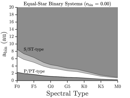
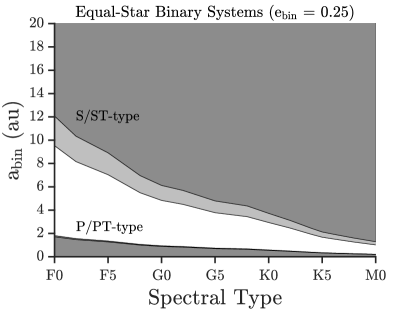
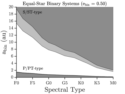
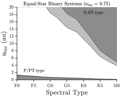
Fig. 1 : Case study 1: Calculated HZs and DZs for equal-mass (and identical spectral type) stellar binary systems ($M_{1}=$ $M_{2}=$ $M$) for different masses, $M$, corresponding to spectral types ranging from F0 to M0 at selected binary eccentricities ($e_{\rm bin}$ = 0.00, 0.25, 0.50, and 0.75). The gray regions indicate the different possible HZs (i.e., S/ST-type and P/PT-type) with the white regions in between illustrating the DZs. The dark and light gray regions correspond to the adopted definitions of GHZ and OHZ, respectively, assuming an Earth-mass planet.

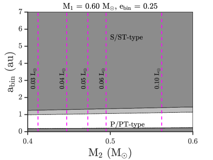
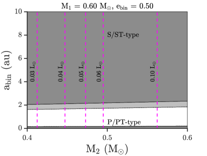
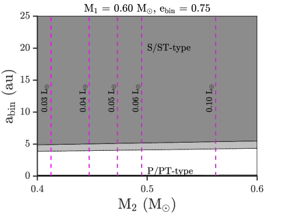
Fig. 2 : Case study 2: Calculated HZs and DZs for a stellar binary system consisting of a primary ($M_{1}=0.60$ $M_{\mathrm{\odot}}$) with a variable mass secondary companion ($M_{2}$) at selected binary eccentricities ($e_{\rm bin}$ = 0.00, 0.25, 0.50, and 0.75). The gray regions indicate the different possible HZs (i.e., S/ST-type and P/PT-type) with the white regions in between illustrating the DZs. The dark and light gray regions correspond to the adopted definitions of GHZ and OHZ, respectively, assuming an Earth-mass planet. The vertical dotted lines (magenta) convey lines of secondary companion luminosity, $L_{2}$.

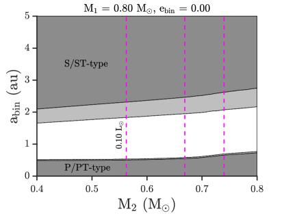
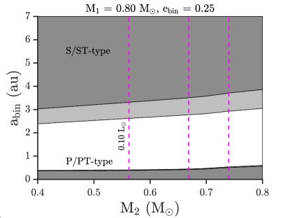
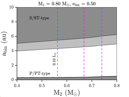
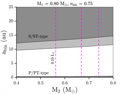
Fig. 3 : Case study 2: Same as Fig. 2, but for a primary of $M_{1}=0.80$ $M_{\mathrm{\odot}}$ and secondary companion luminosity, $L_{2}$, in increments of 0.10 $L_{\mathrm{\odot}}$, with the luminosity increasing from left to right.

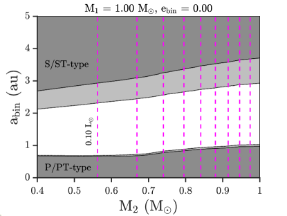
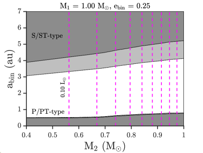
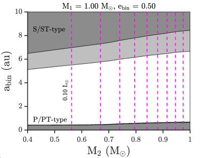
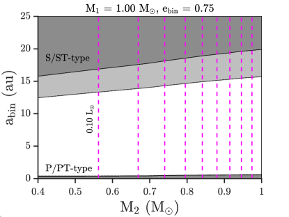
Fig. 4 : Case study 2: Same as Fig. 3, but for a primary of $M_{1}=1.00$ $M_{\mathrm{\odot}}$.

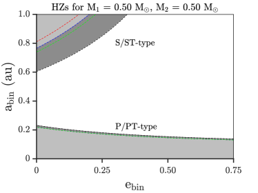
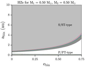
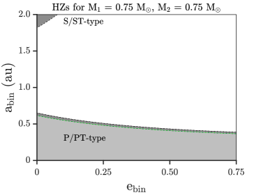
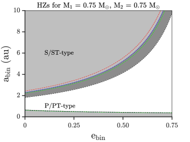
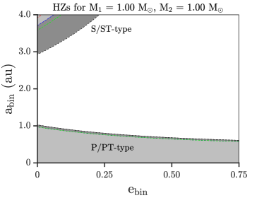
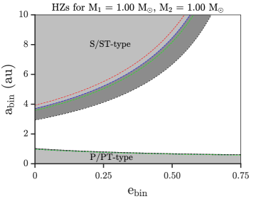
Fig. 5 : Case study 3: Calculated HZs and DZs for three equal-mass stellar binary systems where $M_{1}$ = $M_{2}$ = 0.50, 0.75, and 1.00 $M_{\mathrm{\odot}}$. The gray regions indicate the different possible HZs (i.e., S/ST-type and P/PT-type) with the white regions in between illustrating the DZs. The dark and light gray regions correspond to the adopted definitions of GHZ and OHZ, respectively, assuming an Earth-mass planet; these definitions are also represented by black-dotted lines (OHZ) and blue-dotted lines (GHZE). Additionally, the red-dotted and green-dotted lines illustrate the GHZ regions assuming a Mars-mass (GHZM) and super-Earth-mass planet (GHZSE), respectively.

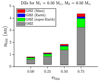
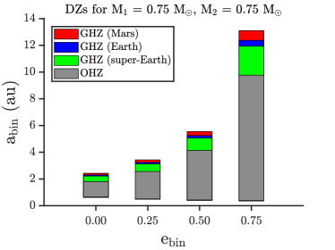
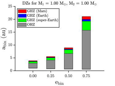
Fig. 6 : Case study 3: DZ widths for the three equal-mass stellar binary systems shown at selected binary eccentricities ($e_{\rm bin}$ = 0.00, 0.25, 0.50, and 0.75). The gray region indicates the OHZ, whereas the red, blue, and green regions correspond to the GHZM, GHZE, and GHZSE case study, respectively.

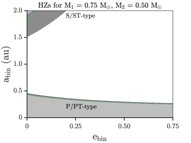
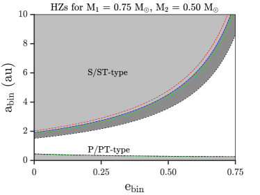
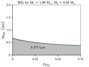
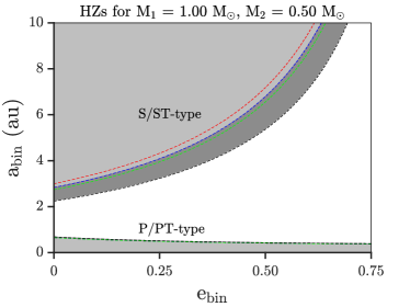
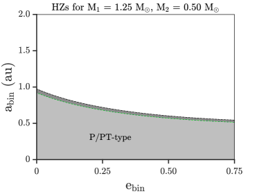
Fig. 7 : Case study 3: Same as Fig. 5, but for three nonequal-mass stellar binary systems where $M_{1}$ = 0.75, 1.00, and 1.25 $M_{\mathrm{\odot}}$ and $M_{2}$ = 0.50 $M_{\mathrm{\odot}}$.

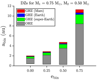
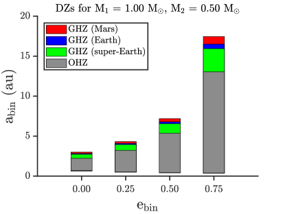
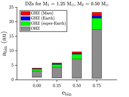
Fig. 8 : Case study 3: Same as Fig. 6, but for three nonequal-mass stellar binary systems where $M_{1}$ = 0.75, 1.00, and 1.25 $M_{\mathrm{\odot}}$ and $M_{2}$ = 0.50 $M_{\mathrm{\odot}}$.

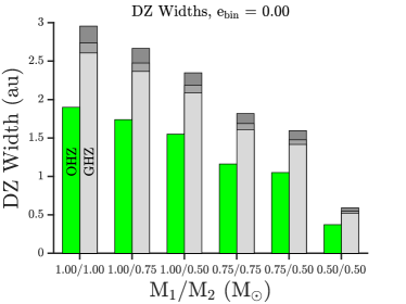
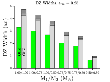
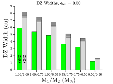
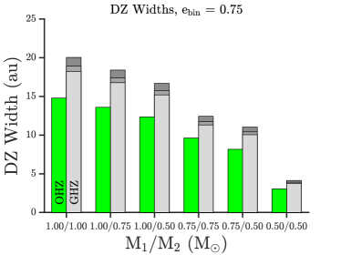
Fig. 9 : Case study 3: DZ widths for several stellar binary systems at selected binary eccentricities ($e_{\rm bin}$ = 0.00, 0.25, 0.50, and 0.75). The gray regions indicate the different DZs corresponding to the GHZ criterion with light, medium, and dark gray corresponding to super-Earth-mass, Earth-mass, and Mars-mass planets, respectively. The green regions represent the OHZ criterion; following Kopparapu et al. (2014) (see text), it does not depend on the planetary mass. The horizontal axes convey the stellar binary systems in terms of primary and secondary mass ($M_{1}/M_{2}$) with the vertical axes illustrating the binary semi-major axes, $a_{\mathrm{bin}}$.

References

- Arney (2019) Arney, G.N.: Astrophys. J. Lett. 873, L7 (2019)
- Bains (2004) Bains, W.: Astrobiol. 4, 137 (2004)
- Barnes et al. (2009) Barnes, R., Jackson, B., Greenberg, R., Raymond, S.N.: Astrophys. J. Lett. 700, L30 (2009)
- Chabrier (2003) Chabrier, G.: Publ. Astron. Soc. Pac. 115, 763 (2003)
- Cockell et al. (2016) Cockell, C.S., Bush, T., Bryce, S., et al.: Astrobiol. 16, 89 (2016)
- Cuntz (2014) Cuntz, M.: Astrophys. J. 780, 14 (2014)
- Cuntz (2015) Cuntz, M.: Astrophys. J. 798, 101 (2015)
- Cuntz & Guinan (2016) Cuntz, M., Guinan, E.F.: 2016, Astrophys. J. 827, 79 (2016)
- Des Marais et al. (2008) Des Marais, D.J., Nuth III., J.A., Allamandola, L.J., et al.: Astrobiol. 8, 715 (2008)
- Duquennoy and Mayor (1991) Duquennoy, A., Mayor, M.: Astron. Astrophys. 248, 485 (1991)
- Dvorak (1982) Dvorak, R.: Österreichische Akad. Wissenschaften Math. Naturwissenschaftl. 191, 423 (1982)
- Eggenberger et al. (2004) Eggenberger, A., Udry, S., Mayor, M.: Astron. Astrophys. 417, 353 (2004)
- Gallet et al. (2017) Gallet, F., Charbonnel, C., Amard, L., Brun, S., Palacios, A., Mathis, S.: Astron. Astrophys. 597, A14 (2017)
- Heller and Armstrong (2014) Heller, R., Armstrong, J.: Astrobiol. 14, 50 (2014)
- Heller and Barnes (2013) Heller, R., Barnes, R.: Astrobiol. 13, 18 (2013)
- Jones et al. (2005) Jones, B.W., Underwood, D.R., Sleep, P.N.: Astrophys. J. 622, 1091 (2005)
- Kaltenegger (2017) Kaltenegger, L.: Annu. Rev. Astron. Astrophys. 55, 433 (2017)
- Kasting et al. (1993) Kasting, J.F., Whitmire, D.P., Reynolds, R.T.: Icarus 101, 108 (1993)
- Kasting and Catling (2003) Kasting, J.F., Catling, D.: Annu. Rev. Astron. Astrophys. 41, 429 (2003)
- Kopparapu et al. (2013) Kopparapu, R.K., Ramirez, R., Kasting, J.F., et al.: Astrophys. J. 765, 131; Erratum 770, 82 (2013)
- Kopparapu et al. (2014) Kopparapu, R.K., Ramirez, R.M., SchottelKotte, J., et al.: Astrophys. J. 787, L29 (2014)
- Kroupa (2001) Kroupa, P.: Mon. Not. R. Astron. Soc. 322, 231 (2001)
- Kroupa (2002) Kroupa, P.: Science 295, 82 (2002)
- Lammer et al. (2009) Lammer, H., Bredehöft, J.H., Coustenis, A., et al.: Astron. Astrophys. Rev. 17, 181 (2009)
- Lingam and Loeb (2018) Lingam, M., Loeb, A.: Internat. J. Astrobiol. 17, 116 (2018)
- Mann et al. (2013) Mann, A.W., Gaidos, E., Ansdell, M.: Astrophys. J. 779, 188 (2013)
- Meadows et al. (2018) Meadows, V.S., Reinhard, C.T., Arney, G.N., et al.: Astrobiol. 18, 630 (2018)
- Moorman et al. (2019) Moorman, S.Y., Quarles, B.L., Wang, Zh., Cuntz, M.: Internat. J. Astrobiol. 18, 79 (2019)
- Olson et al. (2018) Olson, S.L., Schwieterman, E.W., Reinhard, C.T., et al.: Astrophys. J. Lett. 858, L14 (2018)
- Patience et al. (2002) Patience, J., White, R.J., Ghez, A.M., et al.: Astrophys. J. 581, 654 (2002)
- Pilat-Lohinger et al. (2019) Pilat-Lohinger, E., Eggl, S., Bazsó, Á.: Planetary Habitability in Binary Systems. Advances in Planetary Science, Vol. 4, World Scientific Publ., Singapore (2019)
- Quarles et al. (2018) Quarles, B., Satyal, S., Kostov, V., Kaib, N., Haghighipour, N.: Astrophys. J. 856, 150 (2018)
- Raghavan et al. (2006) Raghavan, D., Henry, T.J., Mason, B.D., et al.: Astrophys. J. 646, 523 (2006)
- Raghavan et al. (2010) Raghavan, D., McAlister, H.A., Henry, T.J., et al.: Astrophys. J. Suppl. Ser. 190, 1 (2010)
- Ramirez (2018) Ramirez, R.M.: Geosciences 8, 280 (2018)
- Roell et al. (2012) Roell, T., Neuhäuser, R., Seifahrt, A., Mugrauer, M.: Astron. Astrophys. 542, A92 (2012)
- Schwieterman et al. (2018) Schwieterman, E.W., Kiang, N.Y., Parenteau, M.N., et al.: Astrobiol. 18, 663 (2018)
- Seager et al. (2016) Seager, S., Bains, W., Petkowski, J.J.: Astrobiol. 16, 465 (2016)
- Underwood et al. (2003) Underwood, D.R., Jones, B.W., Sleep, P.N.: Internat. J. Astrobiol. 2, 289 (2003)
- Wang and Cuntz (2019a) Wang, Zh., Cuntz, M.: Astrophys. J. 873, 113 (2019a)
- Wang and Cuntz (2019b) Wang, Zh., Cuntz, M.: Res. Not. Am. Astron. Soc. 3e, 70 (2019b)
- Williams and Pollard (2002) Williams, D.M., Pollard, D.: Internat. J. Astrobiol. 1, 61 (2002)