Softening of DNA near Melting as Disappearance of an Emergent Property
Abstract
Near the melting transition the bending elastic constant , an emergent property of double-stranded DNA (dsDNA), is shown not to follow the rodlike scaling for small length . The reduction in with temperature is determined by the denatured bubbles for a continuous transition, e.g., when the two strands are Gaussian, but by the broken bonds near the open end in a Y-like configuration for a first-order transition as for strands with excluded volume interactions. In the latter case, a lever rule is operational implying a phase coexistence although dsDNA is known to be a single phase.
I Introduction
DNA stores the genetic information in its base sequence, but its functionality relies on its physical properties, like stiffness and length. The elastic energy of DNA packaged in a viral capsid helps in the injection processpurohit ; garcia , energetically-costly bends of DNA provide sites for attachments of transcription factors and other enzymeshori ; rees ; topoiso , while the melting of DNA is a vital step in polymerase chain reactionsmullis . The topological constraint when double-stranded DNA (dsDNA) is viewed as a ribbon, leads to two independent elastic constants for twist and bendvologo ; hager ; dietler ; abels . Both these elastic constants vanish on the melting of dsDNAbrunet ; vologo ; olson , when the ribbon picture is lost, showing that the stiffness is an emergent property of the bound DNAkivelson . However, how this emergent behaviour goes away at melting is still unknown. Here we determine the fundamental relation between the emergent bending elastic constant and the fraction of broken base-pairs that drives the melting transition. We show, by simulating long semiflexible DNA, that the relation is dependent on the order of the melting transition, and involve different physical mechanisms.
For a continuous melting transition, as for Gaussian chains, a renormalized semiflexible chain picture is valid where effective for long chains is renormalized non-trivially by the fraction of broken bonds. Melting is found to occur homogeneously along the chain but a worm-like chain model is applicable only at low temperatures where there are no broken pairs. In contrast, in the presence of excluded volume interaction, when melting is first order, the effective is found to be determined by a phase-coexistence type picture with the reduction in rigidity coming mainly from the large fraction of broken bonds near the open end of dsDNA. It is not homogeneous melting, and a phase-coexistence is at odds with the conventional mechanism of bubble-induced melting transition.
The stiffness of dsDNA is expressed in terms of the persistence lengthhager ; dietler ; abels nm which is much larger than that of highly flexible individual strands of DNA (ssDNA) with nm. Generally, at temperature is defined on dimensional ground from the bending elastic constant as (the Boltzmann constant ), whereas the intuitive picture that a semiflexible polymer behaves like a rod for lengths less than , follows from the decay length of the tangent-tangent correlation function, where is the tangent to the space curve at monomer as shown in Fig. 1, is the bond length, and denotes ensemble average. These two definitions match for a worm-like chain which is Gaussian at long length, but not in the presence of excluded volume interaction when decays as a power-law without any typical lengthhager ; schafer ; hsu .
As the base-pair energy - kcal/mol, thermal fluctuations lead to a cooperative breaking of the hydrogen bonds in the long length limit. This is the melting of DNAvologodski3 . The broken base pairs may be distributed along the chain or maybe near the open end (called the Y-fork) when one end of DNA is kept fixed. A consecutive set of broken pairs is to be called a bubble; see Fig. 2. This bubble mediated transition is the usual Poland-Scheraga scheme of thermal melting of DNAfisher . The fraction of unbroken bonds play the role of the order-parameter for the transition, viz., in the dsDNA (denatured) phase, and depending on the nature of the interactions, the melting transition can be continuous or first-orderfisher ; causo . As the ssDNA’s are flexible, the bubbles act as hinges for the rigid segmentsyan ; forties ; wiggins ; vologodskii2 ; palsmb ; bonnet ; vologo , and, additionally, bubbles have biologically important roles chongli ; ramstein . The extra flexibility introduced by the bubbles leads to a downward renormalization of the elastic constant as shown schematically in Fig. 1, provided the bubbles are distributed homogeneously along the chain. The loss of stiffness of dsDNA is gradual over a range of C near melting brunet , but the validity of the homogeneous picture and the functional form of the temperature dependence are not known. There is also a problem in defining or a “ribbon” at higher temperatures for configurations dotted with bubbles (Fig. 1), unless one coarse-grains at the scale of the bubble size.
Why is dsDNA stiff when individual strands are not and how does that stiffness go away with the increase of temperature? These questions may resemble similar ones about the rigidity of crystals. However, there are fundamental differences between the two cases. For a solid, rigidity is also an emergent phenomenon, where the shear modulus, imparting rigidity, is a consequence of continuous-symmetry breakingkivelson . There is no such scenario for , especially because it is not the response function associated with any order-parameter, like . Instead, the bound phase allows a ribbon-like description for which topological argumentsvologo , e.g., the Călugăreanu theorem, are applicable. The twist elastic constant, related to the helical nature, and the bending elastic constant related to the entropy of DNAvologodski3 , are relevant for dsDNA, but not for ssDNA or the denatured phase where the ribbon picture is lost. Of the two elastic constants, is a large scale property that should be insensitive to microscopic details, while the twist constant is dependent on the details of the structure. It is, therefore, possible to model the reduction of through the changes in the semiflexible bound structure mediated by the broken base-pairs. The occurrences of bubbles, as in Fig. 1, may seem to invalidate the ribbon picture, even raising questions on defining a tangent vector . These issues may be alleviated by coarse-graining on a scale larger than the bubble size (Fig. 1) restoring the ribbon picture with renormalized elastic constants. With this in mind, we use coarse-grained models for finite length DNA, which are important from experimental point of view, since experiments are performed upon finite system.
This paper is organized in the following manner. In Sec. II the coarse-grained models are defined. Two models, viz., Gaussian chain model and chains with self- and mutual-avoidance, both on a cubic lattice are defined there. The connection of the elastic constant with appropriate sizes via fluctuation theorems are also elaborated there. Sec. III gives the details of the simulation method of developing PERM for dsDNA. Sec. IV discusses the drastic difference in the behaviour of rigidity when excluded volume interactions are taken into account. Sec. V concludes the paper with some analogies between DNA melting and crystal melting.

II Model and Qualitative Description
Two different models are considered here, viz., I and II, on a cubic lattice. In model I, the strands are Gaussian chains, while in model II, we incorporate both self and mutual avoidance. The binding of the chains is allowed by an attractive energy whenever a monomer of one chain is in contact with a monomer of the other chain provided both monomers have the same position along the chain. This ensures the native base-pairing of DNA. In each case, we consider two varieties of polymers, viz., (i) flexible polymers where both the single and double strands are flexible, and (ii) semiflexible dsDNA where only the bound parts are semiflexible but the bubbles consist of flexible chains. The semi-flexibility in dsDNA is incorporated by penalizing a bend of two successive paired bonds with energy where is the angle between two bonds and is the bending energy constant; see Fig. 2(a)-(c). Whereas a bent ds configuration as in Fig. 2(c) is energetically favourable compared to Fig. 2(b), the latter is a source of additional entropy. Consequently, bubbles (Fig. 2(d)) are to be expected at higher temperatures vis-a-vis bent ds-chains at lower temperatures comm3 .
To explore the elastic behaviour, a force is applied at the end point of each strand of length , keeping the other ends fixed. The additional force-term in the Hamiltonian is , where . The elastic response can be defined from a tensorial quantity as , with the subscripts denoting the Cartesian components. In the zero force limit (), isotropy can be used to define the elastic constant as , which can be related to the zero-force fluctuations of as where the averaging is done with the Hamiltonian. This fluctuation relation allows us to determine without any external force. As we see, the bending elastic constant is not the response function associated with and so the conventional critical behaviour of response functions in phase transition problems are not applicable here.

Naively, one may interpret as the variance of the end-to-end distance of the center-of-mass (CM) chain . Therefore, the dependence of is given by the size of the CM chain, with a scaling behaviour . However, the CM chain is not expected to behave like an ordinary polymer, except in special situations, but in case it does so, the size exponent for a Gaussian chain and for a self-avoiding walk (polymers in good solvent). For a semiflexible Gaussian chain, the crossover from for to for , is given byfloryrev
| (1) |
with as the persistence length. Here both and length are measured in units of bond lengths which is set to one. This formula is used often for DNA when the CM chain more or less coincides with the strands, i.e., in absence of bubbles. In general, the temperature dependence of would show us how DNA softens as the melting point is reached.
In terms of the individual coordinates,
| (2) |
is determined by the inter-chain correlation. In the perfect bound state with no bubbles, , and we get , while in the high-temperature phase, if the two chains remain uncorrelated, then is equal to the sum of the individual modulus. Then, , for Gaussian chains. The ratio is expected to be for strands with excluded volume interactions because there will be inter-strand correlations for long chains as dictated by the second virial coefficient (or overlap concentration ) degenne . Moreover, in the bound phase, individual strands also acquire the stiffness of the state, punctuated by bubbles and Y-fork. Therefore, the microscopic stiffness would no longer be the sole parameter determining the overall elasticity of the chain (Fig. 1). In our study, it is assumed that the bending rigidity is isotropic i.e. the bending energy only depends on the angle by which the polymer is bent locally, and do not depend on the direction of bending, although, it has been shown that the bending rigidity in the direction of the grooves is essentially smaller than in the perpendicular directionolson ; zhurkin . To characterize the transition, we computed the fraction of broken bonds in the bubbles and , the fraction in the Y-fork like region. The transition temperature was determined from the specific heat curves; see Appendix A. In all cases, the order of transition is found to be independent of the value of stiffness .
III Simulation Algorithm
For simulation, we have used the zero parameter version of the flatPERM (Pruned and Enriched Rosenbluth Method) which generates equilibrium configurations through cloning and pruningprellberg ; causo . Both the strands are grown simultaneously by considering all the joint possibilities of taking steps together. The weighted atmosphere at each step, i.e., the number of free sites available for the next step, serves as the weight of that step , and the weight of a configuration is the successive multiplication of the weights of the previous steps . For example, for the first step, each of the chains has different possibilities to step into. Of a total of possibilities, there are possible ways of making a contact; thus the local weighted atmosphere becomes . Similarly, the weight for the second step including a bend and excluded volume interaction is . For Gaussian strands, reverse steps in the ds mode with are considered with an appropriate change in . The partition function for chain length is estimated by averaging over the weights of configurations of length with respect to the number of started tours where a tour is a set of chains generated with a rooted tree topology between two successive return to the main() function. An average over tours were used in this study for chain lengths up to and error bars are estimated on the fly; see Appendix D. Pruning and enrichment is done continuously depending on whether the ratio of the weight of the particular configuration and the partition function estimate for length , is smaller or greater than respectively. For ratio the configuration keeps on growing with probability and pruned otherwise. While for we make distinct copies with , where is the total atmosphere and each copy with weight . And for the configuration continues to grow without any pruning or enrichment. The input parameters for the simulations consist of the temperature , contact energy , bending energy constant with throughout the simulation unless otherwise specified. To translate in our simulation to a variation in C in experiments, one requires a proper scaling, e.g. can be estimated by comparing our to the experimental melting temperature.

(a)
 (b)
(b)
IV Results and Discussion
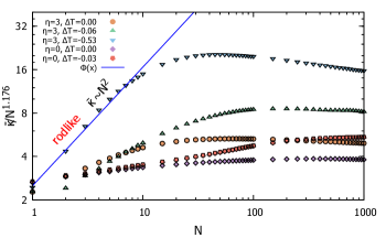
If dsDNA behaves as a semiflexible chain, then for small , as a rigid rod, with a crossover to Gaussian or SAW-like behaviour for large . No rodlike behaviour is seen for . Fig. 3(a) shows that for model I, a tightly bound DNA (without bubbles) at () satisfies Eq. (1) with , consistent with the estimate of from a transfer matrix calculation (see Appendix F). For model II also, at low temperatures, it is possible to define a rodlike behaviour; see Fig. 3(b). However, the crossover description fails near the transition because of substantial contributions from and/or . In the log-log plot, the slope for small lengths is not consistent with the rigid rod expectations. For close to , DNA is neither rodlike nor completely flexible for small chain lengths. We call this region as soft DNA. It follows that though an effective elastic constant can be defined, persistence length from tangent correlations may not have any special significance.
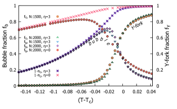
Model I: For Gaussian chains, the melting transition is continuous at for and for . Below melting, bubbles develop, and the fraction of broken bonds, , increases with temperature continuously to 1 as for . For finite chains, there are also broken bonds at the open end, but vs curve sharpens into a step function for . Stiffness on the ds segments has the effect of suppressing the bubble formation at lower temperatures but the continuous transition remains intact. Fig. 4(a) shows the fractions for and .
(a)
 (b)
(b)
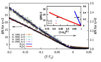
These results are consistent with the Poland-Scheraga picture of DNA melting, that most of the broken bonds are in the bubbles, while the fraction in the Y-region increases for . As the bubbles act like hinges, the decrease of the elastic constant with can be attributed to the broken bonds, thereby renormalizing the effective elastic constant as in Fig. 1. As melting is continuous (see Appendix A and Fig. 4(a)) the change in the elasticity near melting is expected to be a power law for comm2 . The order parameter has the asymptotic behaviour , so that the temperature dependence of elastic constant is . To extend the range of the asymptotic form valid for , we make an ansatz
| (3) |
where is the amplitude, and the exponents and take care of the softening by the bubbles. The values of and are found to give a good agreement of the data shown in Fig. 4(b) when the values of were used from Fig. 4(a). The same picture remains valid for both and . We find for and for . This proposed model for elasticity suggests that the rigidity follows the order parameter curve as the melting point is approached from the bound side.

(a)
 (b)
(b)
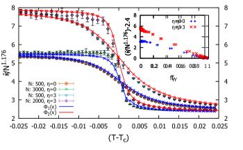
Model II: For self and mutually-avoiding chains the melting transition is first-order at for and for . The temperature dependence of and are shown in Fig. 5(a), while that of in Fig. 5(b), where takes into account the effect of excluded volume interaction (see Eq. (2)). There are significant differences from model I. Close to melting, most of the broken bonds are in the Y-fork, the fraction in the bubbles remains more or less the same. Consequently, Eq. (3), encoding Fig. 1, is not meaningful; but instead an empirical equation, reminiscent of the lever rule in phase coexistence, is found to describe the data. We see a deviation from the Poland-Scheraga picture. Our proposed model for rigidity in this case is based on the superposition of the elastic constant for the bound and the unbound Y-part in the proportion of as
| (4) |
which gives of the bound phase for , and of the unbound phase for with , the two limiting values were adjusted to get a good fit with the values of taken from Fig. 5(a). These points are also shown in the figure. The bubble contribution in the bound part is found to be very small. The temperature independence of the elastic constant on the bound side away from melting is consistent with the experimental results of brunet . The major implication of Eq. (4) is the coexistence of the bound and the unbound state, although dsDNA is a single phase.
We note that the bubble fraction is lower for the semi-flexible models [Figs. 4(a) and 5(a)], and is a manifestation of the coupling between bubble formation and DNA bending energetics (see Fig. 2). For stiffer bonds, it becomes energetically favourable to maintain a bound state and make a straight move than to form a bubble to become flexible; in other words, bending energy of a semi-flexible DNA reduces the possibility of bubble formation. This tendency to maintain the bound state decreases the entropy of the system compared to the case, thereby providing thermal stability to the bound phase. Thus the melting temperature is higher for nonzero , and the transition becomes sharper. However, the bubble size distribution and thus the average bubble length near the transition remain unaltered by stiffness.
V Conclusion
We conclude by comparing the melting picture of DNA with that of a crystal. Two main contenders of the mechanism for melting of a crystal are the homogeneous melting via the formation of defects, topological or nontopological, and a surface meltingyip ; mei . If the defects form anywhere in the bulk crystal due to thermal fluctuations, the ordering is destroyed with a reduction of the rigidity. The melting process is then homogeneous. A different possibility is a surface melting where a wetting liquid layer is formed on the surface and the thickness of the layer diverges at the melting point. We do see analogs of these two processes in DNA melting, though distinctly different in detail, and dependent on the order of the transition. For continuous transitions, it is the Poland-Scheraga scheme of homogeneous bubble formation that modifies the elastic constant as in Eq. (3). For a ribbon picture to be applicable, a coarse-graining as shown in Fig. 1, is necessary. The reduction in rigidity follows the temperature dependence of the fraction of intact bonds. On the other hand, with excluded volume interaction the melting process starts at the open end, like surface melting, at temperatures below the real melting temperature, forming the Y-region. The melting process completes when the length of the Y-region diverges (for infinite chains). In this scenario, for long chains, the density of broken bonds when expressed in terms of the length of the bound segment, viz., should be independent of , as we found to be the case (see Appendix E). This picture also suggests that if a dsDNA is capped by a sequence of high binding energy (i.e. of a higher melting point), then there is a possibility of superheating a dsDNA, when the dsDNA state can be maintained in its bound phase above the melting point. This nonequilibrium aspect is beyond the scope of equilibrium simulations.
Acknowledgements
Computations performed on a FUJITSU high-performance computing facility (SAMKHYA) at the Institute Of Physics Bhubaneswar. SMB acknowledges support from the JCBose Fellowship grant.
(a)
 (b)
(b)
Appendix A Estimation of the Transition point
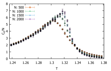
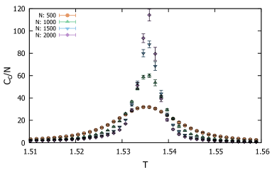
The transition (melting) point has been estimated from the contact number fluctuation per basepair (related to the specific heat). For model I, undergoing a continuous transition, the transition point is determined from the intersection point of the curves for various lengths , that remains invariant under a change of system size (Fig. 6(a)) and the transition point is estimated to be for . For model II which undergoes a first-order transition, the transition point is determined from the peak of the contact number fluctuation curves (Fig. 6(b)), and the transition point is estimated to be for .
Appendix B Bubble Size Distribution
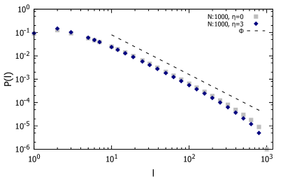
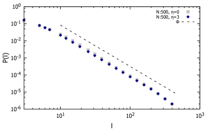
The bubble size distribution at the transition point scales asfisher ; carlon
| (5) |
where is the probability of a bubble of length and the exponent is related to the nature of the transitionfisher . If , it represents a first-order transition, while represents a continuous transition and for there is no transition at all. As per the definition of a bubble, broken bonds in the Y-fork is not included in the bubble statistics. See Fig. 7. The observed slopes are consistent with a continuous transition for Model I (Gaussian chains) but a first-order transition for Model II (chains with excluded volume interaction).
(a)
 (b)
(b)
Appendix C Benchmark for Simulation results
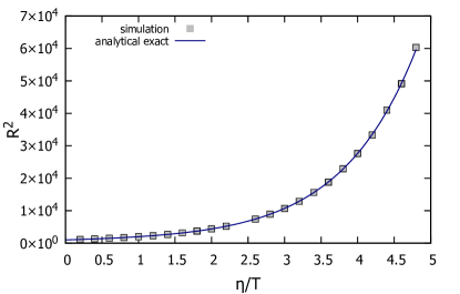
To check for the accuracy of our code in case of semi-flexible Gaussian chains, we calculated the mean squared end-to-end distance for different rigidities at a very low temperature where the DNA is in the bound state, and compared with the exact analytical result for a single ideal semi-flexible chain. Analytically, for an ideal semi-flexible chain the mean squared end-to-end distance varies with the rigidity of the local bending asfloryrev
| (6) |
where
and is the two step partition function when no external force is applied. The comparison is shown in Fig. 8. The form of is specific to our convention of the energetics for polymer bending, where if overlapped (i.e. in the single chain limit) the polymer has the following local partition function for a two step walk
| (7) |
where is for moving straight, for moving backwards and 1 for right angle turns over a cubic lattice according to the bending energy .
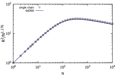
In the presence of self and mutual avoidance, for model II of DNA, a good check would be to compare the size of the polymer chain at a very low temperature (i.e. large ) when the two chains would be completely in the overlapped state and would behave as a single rigid chain, with that of the single chain of the same rigidityhsuS . The comparison is shown in Fig. 9. Note that for both dsDNA and a single self-avoiding chain, the relatve weight for bending is taken as .
Appendix D On the fly error calculation for fluctuating quantities
The estimation of error for any thermodynamical observable is the fluctuation of that quantity. For quantities which are fluctuating in itself e.g. contact number fluctuation or elastic modulus estimation of error becomes tricky. The way PERM is implemented every tour provides an independent estimate of any quantity which contributes to another sample in the running average. Now, with every new estimate from a tour the difference of the present estimate from the estimate of the average up to now gives a measure for the fluctuation of that quantity. The updates of the mean and the fluctuation of a quantity follows the scheme
| (8) | |||||
| (9) |
where is the current th estimate of the quantity, represents the average up to samples and . Thus, the standard deviation is given by
| (10) |
This method is known as Welford’s method.
Appendix E Data collapse for first-order melting
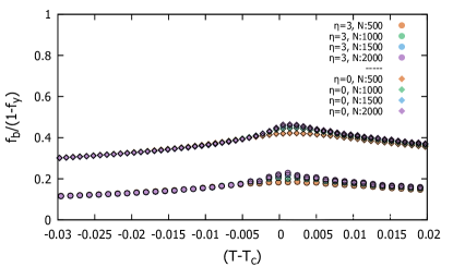
Let and be the total number of broken bonds in bubbles and the Y-fork region. Then and and their temperature dependence is shown in Fig. 5(a). If we treat the chain as consisting of two segments, bound and Y, then the density of broken bonds in the bound segment will be . For long bound segments, should be independent of . The plot of vs in Fig. 10 shows a nice collapse both for and , except for the usual finite size effect near . This data collapse validates the coexistence picture.
Appendix F Transfer Matrix Calculation of Persistence Length
For Gaussian semiflexible chains, the tangent-tangent correlation or bond-bond correlation (Fig. 1) decays exponentially for large , providing a definition for persistence length , where is the bond length. This definition is not applicable for cases with excluded volume interaction, as SAWs are critical objects schafer . The persistence length for model I with at temperature () can be exactly calculated from transfer matrix calculation of a two step walk. The transfer matrix for a two step walk is written as
| (11) |
The largest eigenvalue for the above matrix is , and for the second largest eigenvalue obtained using MATHEMATICA is .Therefore, the persistence length is .
References
- (1) P.K. Purohit, J. Kondev, and R. Phillips. Mechanics of DNA packaging in viruses. Proc. Natl. Acad. Sci. USA 100, 3173-3178 (2003).
- (2) H.G. Garcia, P. Grayson, L. Han, M. Inamdar, J. Kondev, P.C. Nelson, R. Phillips, J. Widom, and P.A. Wiggins. Biological Consequences of Tightly Bent DNA: The Other Life of a Macromolecular Celebrity. Biopolymers 85, 115 (2007).
- (3) M. Horikoshi, C. Bertuccioli, R. Takada, J. Wang, T. Yamamoto, and R.G. Roeder. Transcription factor TFIID induces DNA bending upon binding to the TATA element. Proc. Natl. Acad. Sci. USA 89, 1060-1064 (1992).
- (4) W. Rees, R. Keller, J. Vesenka, G. Yang, and C. Bustamante. Evidence of DNA bending in transcription complexes imaged by scanning force microscopy. Science 260, 1646-1649 (1987).
- (5) S. Lee, S-R. Jung, K. Heo, Jo Ann W. Byl, J.E. Deweese, N. Osheroff, and S. Hohng. DNA cleavage and opening reactions of human topoisomerase II are regulated via Mg2+-mediated dynamic bending of gate-DNA. Proc. Natl. Acad. Sci. USA 109, 2925-2930 (2012).
- (6) K.B. Mullis and F.A. Faloona. Specific Synthesis of DNA in Vitro via a Polymerase-Catalyzed Chain Reaction. Methods Enzymol 155, 335-350 (1987).
- (7) S. Geggier and A. Vologodskii. Sequence dependence of DNA bending rigidity. Proc. Natl. Acad. Sci. USA 107, 15421-15426 (2010).
- (8) P.J. Hagerman. Flexibility of DNA, Ann. Rev. Biophys. Biophys. Chem. 17, 265 (1988).
- (9) K. Rechendorff, G. Witz, J. Adamcik, and G. Dietler. Persistence length and scaling properties of single-stranded DNA adsorbed on modified graphite. J. Chem. Phys. 131, 095103 (2009).
- (10) J.A. Abels, F. Moreno-Herrero, T. van der Heijden, C. Dekker, and N.H. Dekker. Single-Molecule Measurements of the Persistence Length of Double-Stranded RNA. Biophys. J. 88, 2737 (2005).
- (11) A. Brunet, A. et al.. How does temperature impact the conformation of single DNA molecules below melting temperature? Nucl. Acd. Res. 46, 2074 (2018).
- (12) W.K. Olson, A.A. Gorin, X.J. Lu, L.M. Hock, and V.B. Zhurkin. DNA sequence-dependent deformability deduced from protein-DNA crystal complexes. Proc. Natl. Acad. Sci. USA 95, 11163-11168 (1998).
- (13) S. Kivelson and S.A. Kivelson. Defining emergence in physics. npj Quantum Materials 1, 16024 (2016).
- (14) L. Schäfer, A. Ostendorf and J. Hager. Scaling of the correlations among segment directions of a self-repelling polymer chain. J. Phys. A: Math. Gen. 32, 7875 (1999).
- (15) H-P. Hsu, W. Paul and K. Binder. Standard Definitions of Persistence Length Do Not Describe the Local “Intrinsic” Stiffness of Real Polymer Chains. Macromolecules 43, 3094 (2010).
- (16) A. Vologodskii. Biophysics of DNA (Cambridge University Press, Cambridge, UK, 2015).
- (17) Our models differ from other models considered previously, e.g., in palmeri , which considered a distance dependent elastic constant. Our models differ with palmeri in the following respect: (i) Both models I and II incorporate polymeric correlations in bubbles, that change the nature of the melting transition, but this correlation is not present in the model of palmeri . (ii) Our Model II considers excluded volume interaction, both inter and intra strand, which are known to be relevant interactions for polymers, and change the reunion exponents relevant for melting fisher . This interaction is absent in palmeri .
- (18) J. Palmeri, M. Manghi, and N. Destainville. Thermal Denaturation of Fluctuating DNA Driven by Bending Entropy. Phys. Rev. Lett. 99, 088103 (2007).
- (19) M.E. Fisher. Walks, walls, wetting, and melting. J. Stat. Phys. 34, 667 (1984).
- (20) M.S. Causo, B. Coluzzi, and P. Grassberger. Simple model for the DNA denaturation transition. Phys. Rev. E 62, 3958 (1999).
- (21) J. Yan and J.F. Marko. Localized Single-Stranded Bubble Mechanism for Cyclization of Short Double Helix DNA. Phys. Rev. Lett. 93, 108108 (2004).
- (22) R.A. Forties, R. Bundschuh and M.G. Poirier. The flexibility of locally melted DNA. Nucleic Acids Res. 37, (2009).
- (23) P.A. Wiggins, R. Phillips and P.C. Nelson. Exact theory of kinkable elastic polymers. Phys. Rev. E 71, 021909 (2005).
- (24) A. Vologodskii, and M.D. Frank-Kamenetskii. Strong bending of the DNA double helix. Nucleic Acids Res. 41, 6785 (2013).
- (25) G. Altan-Bonnet, A. Libchaber and O. Krichevsky. Bubble Dynamics in Double-Stranded DNA. Phys. Rev. Lett. 90, 138101 (2003).
- (26) T. Pal, T. and S.M. Bhattacharjee. Rigidity of melting DNA. Phys. Rev. E. 93, 052102 (2016).
- (27) C. Yuan, E. Rhoades, X.W. Lou and L.A. Archer. Spontaneous sharp bending of DNA: role of melting bubbles. Nucleic Acids Res. 34, 4554 (2006).
- (28) J. Ramstein and R. Lavery. Energetic coupling between DNA bending and base pair opening. Proc. Natl. Acad. Sci. USA 85, 7231 (1988).
- (29) S.M. Bhattacharjee, A. Giacometti and A. Maritan. Flory Theory for Polymers. J. Phys. Condens. Matter 25, 503101 (2013).
- (30) Here refers to the unbound phase for .
- (31) S.R. Phillpot, S. Yip and D. Wolf. How Do Crystals Melt?. Comp. in Phys. 3, 20 (1989).
- (32) Q.S. Mei and K. Lu. Melting and superheating of crystalline solids: From bulk to nanocrystals. Prog in Mat. Sci. , 52 1175-1262 (2007).
- (33) V.B. Zhurkin, Y.P. Lysov and V.I. Ivanov. Anisotropic flexibility of DNA and the nucleosomal structure. Nucleic Acids Res. 6, 1081 (1979).
- (34) P.G. de Gennes, Scaling Concepts in Polymer Physics (Cornell University Press, Ithaca, NY, 1979).
- (35) T. Prellberg and J. Krawczyk. Flat Histogram Version of the Pruned and Enriched Rosenbluth Method. Phys. Rev. Lett. 92, 120602 (2004).
- (36) E. Carlon, E. Orlandini and A.L. Stella. Roles of stiffness and excluded volume in DNA denaturation. Phys. Rev. Lett., 88, 198101 (2002).
- (37) H-P. Hsu, W. Paul and K. Binder. Polymer chain stiffness vs. excluded volume: A Monte Carlo study of the crossover towards the worm-like chain model. Euro Phys. Lett. 92, 28003 (2010).