Detection of quantum non-Markovianity close to the Born-Markov approximation

Abstract

We calculate in an exact way the conditional past-future correlation for the decay dynamics of a two-level system in a bosonic bath. Different measurement processes are considered. In contrast to quantum memory measures based solely on system propagator properties, here memory effects are related to a convolution structure involving two system propagators and the environment correlation. This structure allows to detect memory effects even close to the validity of the Born-Markov approximation. An alternative operational-based definition of environment-to-system backflow of information follows from this result. We provide experimental support to our results by implementing the dynamics and measurements in a photonic experiment.

Decoherence and dissipation are phenomena induced by the unavoidable coupling of an open quantum system with its environment. When describing this kind of system dynamics some important approximations are usually considered. A paradigmatic example is the Born-Markov approximation (BMA), which considers that the reservoir is not altered significantly due to the presence of the system. The BMA has been used extensively, providing excellent agreement with many experiments such as for example in the context of quantum optics and magnetic resonance.

The high degree of control on individual quantum systems achieved in the last years leads to the necessity of characterizing dynamics beyond the BMA breuerbook ; vega . In this regime, the environmental degrees of freedom are affected and depend on the system state. This property gives the physical ground for a wide class of witnesses and measures of quantum non-Markovianity BreuerReview ; plenioReview , where the system-environment mutual influence is read in terms of an environment-to-system backflow of information piilo ; breuerDecayTLS ; dario ; sabrina ; paris ; acin ; indu ; EnergyBackFLow ; Energy ; HeatBackFLow . This phenomenon has been studied through physical variables such as energy and heat EnergyBackFLow ; Energy ; HeatBackFLow , and observed experimentally in different setups mari ; mfs1 ; mfs2 ; alejandra ; china ; breuerDrift ; flowExp .

Consistently, the definitions of the previous quantum memory measures rely on the system density matrix evolution or propagator, whose properties in fact encode the memory effects induced by the system-environment coupling. Nevertheless, even when a quantum master equation is obtained beyond the BMA, these memory measures may indicate the absence of any non-Markovian effect. For example, dynamics characterized by positive time-dependent decay rates are usually classified as Markovian ones vega ; BreuerReview ; plenioReview .

This drawback is circumvented by operational quantum memory approaches, where different consecutive measurements are performed during the system evolution modi ; pollock ; budini ; budiniChina . Both, a univocal relation between memory effects and departures from BMA, as well as consistence with the classical definition of non-Markovianity are achieved with these techniques. Experimental implementation has been recently performed budiniChina .

In spite of the previous achievements, the understanding of operational quantum memory witnesses is in its early days. In fact, phenomenon like environment-to-system backflow of information and similar memory measures can be completely characterized after knowing the system density matrix evolution. In contrast, we notice that this information is not sufficient to characterize operational approaches, where dynamical memory effects that arise between consecutive measurement processes are not captured by knowing solely the unperturbed system dynamics. The main goal of this contribution is to determine which object may take the role of the system propagator when characterizing operational memory witnesses, which in turn allows to detecting memory effects close to the validity of the BMA.

In this work, by using a conditional past-future (CPF) correlation method, we study memory effects in the decay dynamics of a two-level system coupled to a bosonic environment. Given that this paradigmatic model admits an exact solution, main differences between operational and non-operational memory approaches are deduced. The CPF correlation is a minimal operational memory witness that is defined by the correlation between the outcomes of “past” and “future” system measurement processes when conditioned to a “present” system state budini . We find that, for different measurement schemes, this witness is proportional to a convolution term that involves two system propagators and the bath correlation. This structure only vanishes when approaching the BMA, which elucidates our main guiding question. An alternative formulation of the phenomenon of environment-to-system backflow of information, which involves the measurement processes, follows from this result. We also develop a photonic setup that implements the system channel dynamics, which provides experimental support to our findings. Experimental conditions necessary to achieve resolution close to the Markovian limit are analyzed in detail.

Microscopic dynamics: The decay dynamics of a two-level system induced by a bosonic bath is described by the Hamiltonian breuerbook

$$H_{\mathrm{tot}}=\frac{\omega_{0}}{2}\sigma_{z}+\sum_{k}\omega_{k}b_{k}^{{\dagger}}b_{k}+\sum_{k}(g_{k}\sigma_{+}b_{k}+g_{k}^{\ast}\sigma_{-}b_{k}^{{\dagger}}).$$ (1)

Here, $\sigma_{z}$ is the $z$-Pauli matrix, $\sigma_{+}=\left|{\uparrow}\right\rangle\left\langle{\downarrow}\right|$ and $\sigma_{-}=\left|{\downarrow}\right\rangle\left\langle{\uparrow}\right|$ are the raising and lowering operators of the qubit in the natural basis $\{\left|{\uparrow}\right\rangle,\left|{\downarrow}\right\rangle\}.$ The bosonic operators satisfy the relations $[b_{k},b_{k}^{{\dagger}}]=1.$

We assume that the total initial wave vector is $|\Psi_{0}\rangle=(a\left|{\uparrow}\right\rangle+b\left|{\downarrow}\right\rangle)\otimes|0\rangle,$ where the environment vacuum state is $|0\rangle\equiv\prod_{k}|0\rangle_{k}.$ The qubit state $\rho_{t}$ is obtained by tracing out the environmental degrees of freedom $\rho_{t}=\mathrm{Tr}_{e}[|\Psi_{t}\rangle\langle\Psi_{t}|],$ obtaining, in the interaction picture,

$$\rho_{t}=\left(\begin{array}[]{cc}|a|^{2}|G(t)|^{2}&ab^{\ast}G(t)\\ a^{\ast}bG^{\ast}(t)&1-|a|^{2}|G(t)|^{2}\end{array}\right).$$ (2)

The operator $\rho_{t}$ fulfills the non-Markovian master equation $(d\rho_{t}/dt)=\frac{-i}{2}\omega(t)[\sigma_{z},\rho_{t}]+\gamma(t)([\sigma_{-}\rho_{t},\sigma_{+}]+[\sigma_{-},\rho_{t}\sigma_{+}]).$ The time-dependent decay rate and frequency are defined as $\gamma(t)+i\omega(t)=-(d/dt)\ln[G(t)].$ The “wave vector propagator” $G(t)$ obeys the convoluted evolution

$$\frac{d}{dt}G(t)=-\int_{0}^{t}f(t-t^{\prime})G(t^{\prime})dt^{\prime},$$ (3)

where the memory kernel is defined by the bath correlation $f(t)\equiv\sum_{k}|g_{k}|^{2}\exp[+i(\omega_{0}-\omega_{k})t].$

Non-operational memory witnesses: As is well known breuerDecayTLS for the model (1), standard memory witnesses such as the trace distance between initial states and departure from divisibility, coincide. In fact, the dynamics is considered Markovian if the rate $\gamma(t)$ is positive. Equivalently, this means that $|G(t)|^{2}$ decays monotonically, giving place to a monotonous decay from the upper level $\left|{\uparrow}\right\rangle$ to the lower state $\left|{\downarrow}\right\rangle.$ Nevertheless, this regime is not necessarily within the BMA.

Operational memory witness: Memory effects defined from a CPF correlation budini rely on three system measurement processes. They are performed at successive times $t_{x}<t_{y}<t_{z}$ during the system dynamics. The CPF measures the correlation between future and past outcomes, labeled by indexes $z$ and $x$ respectively, when conditioned to a given fixed outcome $y$ at the intermediate present time. Explicitly,

$$C_{pf}(t,\tau)|_{y}=\sum_{zx}[P(z,x|y)-P(z|y)P(x|y)]O_{z}O_{x},$$ (4)

where in general $P(b|a)$ denotes the conditional probability of $b$ given $a.$ Furthermore, $t\equiv t_{y}-t_{x}$ and $\tau\equiv t_{z}-t_{y}$ are the time elapsed between consecutive measurements. $\{O_{z}\}$ and $\{O_{x}\}$ are the (eigen) values of the measured quantum observables.

The CPF correlation intrinsically depends on which measurement processes are performed at each time. Here, we consider projective measurements performed in different directions $\hat{n}$ in the Bloch sphere. Thus, $x=\pm 1,$ $y=\pm 1,$ $z=\pm 1$, while $O_{z}=z,\ O_{x}=x.$ Considering the initial state $|\Psi_{0}\rangle$, $t_{x}=0$, and the unitary dynamics associated to Eq. (1), we calculate the exact CPF for two different sets of directions $\hat{n}$ suppl . For the directions $\hat{z}$-$\hat{z}$-$\hat{z},$ the CPF correlation when conditioned to $y=-1$ reads

$$C_{pf}(t,\tau)|_{y=-1}\underset{\hat{z}\hat{z}\hat{z}}{=}\left\{\frac{4|a|^{2}|b|^{2}}{[(1-|G(t)|^{2})|a|^{2}+|b|^{2}]^{2}}\right\}|G(t,\tau)|^{2}.$$ (5)

Alternatively, by performing successive measurements in the $\hat{x}$-$\hat{z}$-$\hat{x}$ directions, for conditional $y=-1,$ it becomes

$$C_{pf}(t,\tau)|_{y=-1}\underset{\hat{x}\hat{z}\hat{x}}{=}-\left\{\frac{1-[2\mathrm{Re}(ab^{\ast})]^{2}}{1-|G(t)|^{2}/2}\right\}\mathrm{Re}[G(t,\tau)].$$ (6)

In the previous two expressions, the function $G(t,\tau)$ is

$$G(t,\tau)\equiv\int_{0}^{t}dt^{\prime}\int_{0}^{\tau}d\tau^{\prime}f(\tau^{\prime}+t^{\prime})G(t-t^{\prime})G(\tau-\tau^{\prime}).$$ (7)

Apart from normalization factors proportional to the initial system state ($a$ and $b$) and the propagator $G(t)$, both Eqs. (5) and (6) are proportional to $G(t,\tau)$ CPFCero . Thus, in contrast to previous approaches, instead of $G(t),$ the memory effects here are determined by this other contribution. It consists in a convolution involving two system propagators mediated by the environment correlation. It is simple to check that $G(t,\tau)\rightarrow 0$ when $f(t)$ approaches a delta function. Consequently, $G(t,\tau)$ measures departures with respect to the BMA, even close to its validity. Interestingly, this factor has a simple physical operational meaning.

Backflow of information: Given that the underlying dynamics admits an exact treatment, a simple relation between a non-operational backflow of information breuerDecayTLS and an operational one can be established as follows: Let us consider that the system is at the initial time in the upper state, a non-monotonous decay of the conditional probability $P(\uparrow,t|\uparrow,0)=|G(t)|^{2}$ determines the presence of an environment-to-system backflow of information (non-operational way). In contrast, under the same initial condition, an operational backflow of information can be defined by the conditional probability $P(\uparrow,t+\tau|\downarrow,t;\uparrow,0)=|G(t,\tau)|^{2}/[1-|G(t)|^{2}]$ suppl which measures the capacity of the environment of reexciting the system given that it has been found in the lower state at an intermediate time. The previous equality univocally defines the operational meaning of $G(t,\tau),$ which in turn guarantees that $P(\uparrow,t+\tau|\downarrow,t;\uparrow,0)$ only vanishes in the Markovian limit [Eq. (7)]. These two clearly different physical scenarios determine the possibility of detecting or not memory effects close to BMA, which in turn may be read as different notions of environment-to-system backflow of information. These results can be generalized by considering other possible system states at the initial and final times $[t=0$ and $(t+\tau)$ respectively]. In fact, this degree of freedom leads to different dependences of the CPF correlation on $G(t,\tau),$ Eqs. (5) and (6).

Decay channel dynamics: In order to demonstrate the experimental feasibility of measuring memory effects close to the BMA, we develop a photonic platform that simulates the non-Markovian system dynamics. The CPF correlation is measured through the sequence $X\rightarrow U(t)\rightarrow Y\rightarrow U(\tau)\rightarrow Z,$ where $X,$ $Y,$ and $Z$ are the measurement processes while $U(t)$ and $U(\tau)$ are the unitary transformation maps associated to the total Hamiltonian (1). These maps represent the system-environment total changes between consecutive measurement processes. Although the real environment is composed of an infinite number of modes, the system reduced dynamical map can be obtained if the environment is regarded also as a two-level system nielsen . The map $U(t)$ is defined by the transformations

$$\left|{\downarrow}\right\rangle\otimes\left|{0}\right\rangle \rightarrow\left|{\downarrow}\right\rangle\otimes\left|{0}\right\rangle,$$ (8a)

$$\left|{\uparrow}\right\rangle\otimes\left|{0}\right\rangle \rightarrow\cos(2\theta)\left|{\uparrow}\right\rangle\otimes\left|{0}\right\rangle+\sin(2\theta)\left|{\downarrow}\right\rangle\otimes\left|{1}\right\rangle.$$ (8b)

Here, $$\left|{0}\right\rangle \left|{1}\right\rangle \theta \cos(2\theta)=G(t). U(\tau)$$ and represent the bath in its ground state and (first) excited state respectively. The angle is such that Eq. (8) is an amplitude damping channel nielsen . Given that the intermediate (second) measurement may leave the system in its ground state and the bath in an excited state, the channel associated to is defined as

$$\left|{\downarrow}\right\rangle\otimes|0\rangle \rightarrow \left|{\downarrow}\right\rangle\otimes|0\rangle,$$ (9a)

$$\left|{\uparrow}\right\rangle\otimes|0\rangle \rightarrow \cos(2\tilde{\theta})\left|{\uparrow}\right\rangle\otimes|0\rangle+\sin(2\tilde{\theta})\left|{\downarrow}\right\rangle\otimes|1\rangle,$$ (9b)

$$\left|{\downarrow}\right\rangle\otimes|1\rangle \rightarrow \sin(2\tilde{\theta}^{\prime})\left|{\uparrow}\right\rangle\otimes|0\rangle+\cos(2\tilde{\theta}^{\prime})\left|{\downarrow}\right\rangle\otimes|1\rangle.\ \ \ \$$ (9c)

This extended damping channel involves one extra initial state, which takes into account the capacity of the environment of reexciting the system after it has been found in the ground state. In fact, the angles are given by the relations $$\cos(2\tilde{\theta})=G(\tau), \sin(2\tilde{\theta}^{\prime})=G(t,\tau)/\sqrt{1-|G(t)|^{2}}$$ and suppl .

The previous maps can be experimentally simulated by encoding the system states $\{|{\downarrow\rangle},\left|{\uparrow}\right\rangle\}$ into polarization of photons $\{|{H\rangle},\left|{V}\right\rangle\},$ while the bath states are encoded into the path degree of freedom of photons. Angles $\{\theta,\tilde{\theta},\tilde{\theta}^{\prime}\}$ are chosen as a function of the simulated bath properties brasil ; rio , where, consistently with Eqs. (8) and (9), a real bath correlation is assumed $[G(t)\in\mathbb{R}].$

Experimental setup: The specific experimental setup is illustrated in Fig. 1. A continuous-wave (CW) laser, centered at 325 nm, is sent to a beta-barium-borate (BBO) crystal. Degenerated pairs of photons (wavelength centered at 650 nm), are produced in the modes signal “s” and idler “i” via spontaneous-parametric-down-conversion Kwiat99 . The photons in mode i are sent directly to detection as they only herald the presence of photons in mode s, while the photons in mode s pass through nested interferometers, which emulate the maps $U(t)$ and $U(\tau)$ rio . Projective measurements are introduced in modules $X,$ $Y,$ $Z.$ The CPF correlation is extracted by using coincidence counts in each projection set.

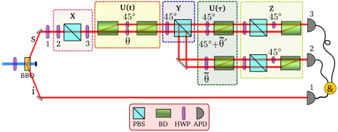
Figure 1: Experimental Setup. Modules $X,$ $Y,$ and $Z$ perform the projective measurements. Modules $U(t)$ and $U(\tau)$ implement the unitary system-environment maps. From coincidence counting, the avalanche photon detectors (APD) allow measuring the CPF correlation (see text).

Given that the photons created in the BBO crystal are horizontally polarized, we prepare any initial linear polarization state $(a\left|{H}\right\rangle+b\left|{V}\right\rangle,\quad a,b\in\mathbb{R})$ using a half-wave plate (HWP₁). The past measurement $X$ is performed using a set of two HWPs and a polarizing beam-splitter (PBS), which transmits the horizontal polarization and reflects the vertical one. In this measurement, the angle set in HWP₂ selects the linear polarization state mapped to $H$ and hence transmitted by the PBS, while HWP₃ prepares the projected state from the transmitted horizontal polarization. After this module, the map $U(t)$ [Eq. (8)] is implemented by coupling the polarization with the path degrees of freedom. For this, we use an interferometer composed of two beam-displacers (BD), each transmitting (deviating) the vertical (horizontal) polarization, and two HWPs, one at each path mode. HWP_θ rotates the polarization so that photons exit the interferometer in (spatial) mode $|0\rangle$ (upper path) or in mode $|1\rangle$ (lower path), depending on $\theta$. HWP_45º simply rotates the photons from $H$ to $V,$ such that all photons of this mode are mapped to mode $|0\rangle$ at the output of the interferometer. Posteriorly, measurement $Y$ is performed using a HWP and a PBS. We restrict ourselves to perform projections in the $\sigma_{z}$ basis. This is done by fixing a HWP at 45º to correct the polarization state such that the $H$-polarized photons are transmitted and $V$-polarized ones are reflected. The map $U(\tau)$ [Eq. (9)], characterized by angles $\tilde{\theta}$ and $\tilde{\theta}^{\prime},$ is implemented in a similar way, noticing that slightly different dynamics take place depending on the result of the Y measurement ($|\downarrow\rangle$ or $|\uparrow\rangle$, equivalent here to transmitted or reflected). The photons on both paths are coherently combined at the two BD. The final $Z$ measurement is also implemented by two sets of HWP and PBS, one set for the transmitted light and the other to the reflected light. The last two BDs, which are just before the detectors Det₂ and Det₃, are used to trace out the path degrees of freedom.

From an experimental viewpoint, to condition the probabilities on the result $y$ of the intermediate measurement is to consider only the coincidence counts between Det₁ and Det₃ (Det₁ and Det₂) for $y=-1$ ($y=+1$). Let $N_{z,x}^{(j)}$ denotes the number of coincidences registered between Det₁ and Det_j when the past and future projective measurements are set to $x$ and $z$ correspondent eigenvectors, respectively. The probabilities used to calculate the CPF correlation (4) can be obtained as $P(z,x|y)=N_{z,x}^{(j)}/\left(\sum_{x^{\prime},z^{\prime}}N_{z^{\prime},x^{\prime}}^{(j)}\right)$, while $P(z|y)=\sum_{x}P(z,x|y)$ and $P(x|y)=\sum_{z}P(z,x|y)$.

Detection of memory effects close to the BMA: The developed platform allows the simulation of the non-Markovian decay dynamics after knowing the environment properties. As a concrete example, we consider a bath with a Lorentzian spectral density, which implies the exponential correlation $f(t)=(\gamma/2\tau_{c})\exp[-|t|/\tau_{c}].$ In this case, the propagator (3) reads

$$G(t)=e^{-t/2\tau_{c}}\Big{[}\cosh(\frac{t\chi}{2\tau_{c}})+\frac{1}{\chi}\sinh(\frac{t\chi}{2\tau_{c}})\Big{]},$$ (10)

where $\chi\equiv\sqrt{1-2\gamma\tau_{c}}.$ Furthermore, Eq. (7) becomes

$$G(t,\tau)=\frac{2\gamma\tau_{c}}{\chi^{2}}e^{-(t+\tau)/2\tau_{c}}\sinh(\frac{t\chi}{2\tau_{c}})\sinh(\frac{\tau\chi}{2\tau_{c}}).$$ (11)

In the weak coupling limit $\gamma\ll 1/\tau_{c},$ where the correlation time $\tau_{c}$ of the bath is the minor time scale of the problem, it follows that $G(t)\simeq\exp[-\gamma t/2],\ G(t,\tau)\simeq 0,$ which in turn implies that, independently of the measurement scheme, a Markovian limit is approached $C_{pf}(t,\tau)|_{y}\simeq 0.$

In Fig. 2 we plot both the theoretical results (full lines) as well as the experimental ones (symbols) for the CPF correlation at equal times, $C_{pf}(t,t)|_{y=-1}.$ Both the $\hat{z}$-$\hat{z}$-$\hat{z}$ [Eq. (5)] and $\hat{x}$-$\hat{z}$-$\hat{x}$ [Eq. (6)] measurement schemes were measured (upper and lower curves respectively). While for the chosen bath correlation parameters the propagator $G(t)$ decays in a monotonous way, detection of memory close to the BMA is confirmed for different bath correlation times $\tau_{c}.$ An excellent agreement between theory and experiment is observed. In particular, at time $t=0,$ null values of the CPF correlation are experimentally observed, meaning that correlation between the system and environment are negligible at the preparation stage budiniChina . While the modulus of $C_{pf}(t,t)|_{y=-1}$ depends on the initial system state,  we note that it is smaller in the $\hat{z}$-$\hat{z}$-$\hat{z}$ scheme when compared with the $\hat{x}$-$\hat{z}$-$\hat{x}$ measurement scheme. In fact, $|G(t,\tau)|^{2}\leq|\mathrm{Re}[G(t,\tau)]|$ [see Eqs. (5) and Eq. (6)]. This feature also reflects that in the former case, in contrast to the last one, the dynamics between measurements is incoherent.

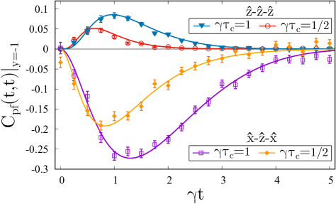
Figure 2: CPF correlation for different projective measurements and bath correlation times. Theoretical results (full lines), experimental results (symbols). The two upper curves correspond to the $\hat{z}$-$\hat{z}$-$\hat{z}$ measurements and the lower ones to $\hat{x}$-$\hat{z}$-$\hat{x}$ measurements. The initial system state is $(\sqrt{p}\left|{\uparrow}\right\rangle+\sqrt{1-p}\left|{\downarrow}\right\rangle)$ with $p=0.8$ (upper curves) and $p=1$ (lower curves). From top to bottom, the bath parameters are $\gamma\tau_{c}=1,$ $1/2,$ $1/2,$ $1.$

We also used the experimental setup for measuring memory effects even closer to the BMA, that is, for smaller bath correlation times. Experimental limitations emerge due to different aspects suppl . For instance, reduced visibility in the interferometers degrades the quality of our operations, weakening agreement between theory and experiment. The finite count statistics also become more relevant when approaching the Markovian limit, as it becomes unclear if a nonnull CPF comes from memory or fluctuation effects. In spite of these limitations, our experiment demonstrates the total feasibility of measuring quantum non-Markovian effects close and beyond the BMA.

Conclusions: Detection of quantum non-Markovianity close to the Born-Markov approximation was characterized through an operational based memory witness. The CPF correlation was calculated for the decay dynamics of a two-level system coupled to a bosonic environment. Instead of the propagator, here the relevant object associated to memory effects consists in the convolution of two system propagators weighted by the environment correlation. This structure can be related to an alternative formulation of the phenomenon of environment-to-system backflow of information, where an intermediate condition on the system state allows to detects memory effects even close to the validity of the BMA. A photonic experiment corroborates the feasibility of detecting quantum memory effects close to the BMA with excellent agreement with the theory.

These results provide a relevant contribution to the understanding of operational-based quantum memory witnesses. In particular, our study elucidates which structure replaces the system propagator when studying these alternative approaches. The validity of the present conclusions to arbitrary system-environment dynamics can be established by using perturbation techniques bonifacio .

Acknowledgments: T.L.S., M.F.S., S.P.W. and G.H.A. acknowledge financial support from the Brazilian agencies CNPq (PQ grants 307058/2017-4, 305384/2015-5, 304196/2018-5 and INCT-IQ 465469/2014-0), FAPERJ (PDR10 E-26/202.802/2016, JCN E-26/202.701/2018, E-26/010.002997/2014, E-26/202.7890/2017), CAPES (PROCAD2013). A.A.B. acknowledges support from Consejo Nacional de Investigaciones Científicas y Técnicas (CONICET), Argentina.

Appendix A System-environment unitary evolution

To calculate the CPF correlation in an exact way, it is necessary to solve the system-environment dynamics for different initial conditions. The total Hamiltonian $H_{\mathrm{tot}}=\frac{\omega_{0}}{2}\sigma_{z}+\sum_{k}\omega_{k}b_{k}^{{\dagger}}b_{k}+\sum_{k}(g_{k}\sigma_{+}b_{k}+g_{k}^{\ast}\sigma_{-}b_{k}^{{\dagger}}),$ in an interaction representation with respect to the uncoupled dynamics becomes

$$H_{\mathrm{tot}}^{I}=\sigma_{+}(t)B(t)+\sigma_{-}(t)B^{\dagger}(t),$$ (12)

where $\sigma_{\pm}(t)=\sigma_{\pm}\exp(\pm i\omega_{0}t),$ and $B(t)=\sum_{k}g_{k}b_{k}\exp(-i\omega_{k}t).$

A.1 Evolution in the time interval $(0,t)$

Let us consider that we can prepare the system-environment in a state

$$|\Psi_{0}\rangle=(a\left|{\uparrow}\right\rangle+b\left|{\downarrow}\right\rangle)\otimes|0\rangle.$$ (13)

Given that the dynamics of both the system and environment is described by the Hamiltonian (12), the state at time $t$ is written as

$$|\Psi_{t}\rangle=\Big{[}a(t)\left|{\uparrow}\right\rangle+b(t)\left|{\downarrow}\right\rangle+\left|{\downarrow}\right\rangle\sum_{k}c_{k}(t)b_{k}^{{\dagger}}\Big{]}|0\rangle.$$ (14)

From Schrödinger equation, the coefficients evolves as $(d/dt)b(t)=0.$ Therefore, $b(t)=b(0)=b.$ In addition, it follows that

$$\frac{d}{dt}a(t) = -i\sum_{k}g_{k}\exp(+i\phi_{k}t)c_{k}(t),$$ (15)

$$\frac{d}{dt}c_{k}(t) = -ig_{k}^{\ast}\exp(-i\phi_{k}t)a(t),$$ (16)

where $\phi_{k}\equiv\omega_{0}-\omega_{k}.$ Integrating the last equation as

$$c_{k}(t)=c_{k}(0)-ig_{k}^{\ast}\int_{0}^{t}dt^{\prime}\exp(-i\phi_{k}t^{\prime})a(t^{\prime}),$$ (17)

the evolution for $a(t)$ becomes

$$\frac{d}{dt}a(t)=-\int_{0}^{t}f(t-t^{\prime})a(t^{\prime})dt^{\prime}-ig(t).$$ (18)

Here, $f(t)$ defines the bath correlation

$$f(t)\equiv\sum_{k}|g_{k}|^{2}\exp(+i\phi_{k}t),$$ (19)

while the inhomogeneous term is

$$g(t)\equiv\sum_{k}g_{k}\exp(+i\phi_{k}t)c_{k}(0).$$ (20)

Defining the Green function $G(t)$ by the evolution

$$\frac{d}{dt}G(t)=-\int_{0}^{t}f(t-t^{\prime})G(t^{\prime})dt^{\prime},$$ (21)

with $G(0)=1,$ the coefficient $a(t)$ can be written as

$$a(t)=G(t)a(0)-i\int_{0}^{t}G(t-t^{\prime})g(t^{\prime})dt^{\prime}.$$ (22)

Initial conditions: Taking the initial conditions

$$a(0)=1,\ \ \ \ \ \ \ c_{k}(0)=0,$$ (23)

which implies $g(t)=0,$ the coefficients can be expressed as

$$a(t)=G(t),\ \ \ \ \ \ c_{k}(t)=-ig_{k}^{\ast}\int_{0}^{t}dt^{\prime}\exp(-i\phi_{k}t^{\prime})G(t^{\prime}).$$ (24)

From Eq. (14) if follows that $|a(t)|^{2}$ is the probability $P(\uparrow,t|\uparrow,0)$ of finding the system in the upper state given that at the initial time $t=0$ it was in the the upper state. From Eq. (24) it follows

$$P(\uparrow,t|\uparrow,0)=|G(t)|^{2}.$$ (25)

A.2 Evolution in the time interval $(t,t+\tau)$

To obtain the CPF correlation, the total evolution must also be solved in the time interval $(t,t+\tau).$ In this case, the state at time $t$ in Eq. (14) plays the role of initial state. Letting the system-environment evolve, the total state can be written as

$$|\Psi_{\tau}\rangle=\Big{[}\tilde{a}(\tau)\left|{\uparrow}\right\rangle+\tilde{b}(\tau)\left|{\downarrow}\right\rangle+\left|{\downarrow}\right\rangle\sum_{k}\tilde{c}_{k}(\tau)b_{k}^{{\dagger}}\Big{]}|0\rangle.$$ (26)

In this case, from the Schrödinger equation we get $(d/d\tau)\tilde{b}(\tau)=0,$ which also implies $\tilde{b}(\tau)=\tilde{b}(0).$ In addition,

$$\frac{d}{d\tau}\tilde{a}(\tau) = -i\sum_{k}g_{k}\exp[+i\phi_{k}(\tau+t)]\tilde{c}_{k}(\tau),$$ (27)

$$\frac{d}{d\tau}\tilde{c}_{k}(\tau) = -ig_{k}^{\ast}\exp[-i\phi_{k}(\tau+t)]\tilde{a}(\tau).$$ (28)

Integrating the last equation, we have

$$\tilde{c}_{k}(\tau)=\tilde{c}_{k}(0)-ig_{k}^{\ast}\int_{0}^{\tau}d\tau^{\prime}\exp[-i\phi_{k}(\tau^{\prime}+t)]\tilde{a}(\tau^{\prime}).$$ (29)

As before, replacing this solution in the previous equation we obtain

$$\frac{d}{d\tau}\tilde{a}(\tau)=-\int_{0}^{\tau}f(\tau-\tau^{\prime})\tilde{a}(\tau^{\prime})d\tau^{\prime}-i\tilde{g}(\tau),$$ (30)

where the inhomogeneous term now is

$$\tilde{g}(\tau)=\sum_{k}g_{k}\exp[+i\phi_{k}(\tau+t)]\tilde{c}_{k}(0).$$ (31)

The coefficient $\tilde{a}(\tau)$ can be written in terms of the propagator $G(t)$ [Eq. (21)] as

$$\tilde{a}(\tau)=G(\tau)\tilde{a}(0)-i\int_{0}^{\tau}G(\tau-\tau^{\prime})\tilde{g}(\tau^{\prime})d\tau^{\prime}.$$ (32)

To calculate the CPF correlation, we have to consider different initial conditions.

First Initial conditions: When

$$\tilde{a}(0)=1,\ \ \ \ \ \ \tilde{c}_{k}(0)=0,$$ (33)

which implies $\tilde{g}(\tau)=0,$ we have the solution

$$\tilde{a}(\tau)=G(\tau),$$ (34a)

while from Eq. (29) we get

$$\tilde{c}_{k}(\tau)=-ig_{k}^{\ast}\int_{0}^{\tau}d\tau^{\prime}\exp[-i\phi_{k}(\tau^{\prime}+t)]G(\tau^{\prime}).$$ (34b)

These solutions are equivalent to the previous ones [Eq. (24)] under the replacement $$t\rightarrow\tau.$$

Second initial conditions: An extra set of initial conditions is given by

$$\tilde{a}^{\prime}(0)=0,\ \ \ \ \ \ \tilde{c}_{k}^{\prime}(0)=c_{k}(t)/\sqrt{1-|G(t)|^{2}},$$ (35)

jointly with $c_{k}(0)=0,$ $a(0)=1$ [Eq. (23)]. This case corresponds to finding the system in its ground state after the second measurement. From Eq. (17) we write $c_{k}(t)=-ig_{k}^{\ast}\int_{0}^{t}dt^{\prime}\exp(-i\phi_{k}t^{\prime})G(t^{\prime}).$ Thus, Eq. (31) becomes

$$\tilde{g}(\tau) = -i\frac{\int_{0}^{t}dt^{\prime}\sum_{k}|g_{k}|^{2}\exp[+i\phi_{k}(\tau+t-t^{\prime})]G(t^{\prime})}{\sqrt{1-|G(t)|^{2}}},$$ (36)

$$= \frac{-i}{\sqrt{1-|G(t)|^{2}}}\int_{0}^{t}dt^{\prime}f(\tau+t-t^{\prime})G(t^{\prime}).$$

From Eq. (32), $\tilde{a}^{\prime}(\tau)=-i\int_{0}^{\tau}G(\tau-\tau^{\prime})\tilde{g}(\tau^{\prime})d\tau^{\prime},$ resulting in

$$\tilde{a}^{\prime}(\tau)=\frac{-\int_{0}^{\tau}d\tau^{\prime}\int_{0}^{t}dt^{\prime}f(\tau^{\prime}+t-t^{\prime})G(\tau-\tau^{\prime})G(t^{\prime})}{\sqrt{1-|G(t)|^{2}}},$$ (37)

which can be rewritten as

$$\tilde{a}^{\prime}(\tau)=\frac{-G(t,\tau)}{\sqrt{1-|G(t)|^{2}}}.$$ (38a)

This equation defines the function $$G(t,\tau).$$ Moreover, from Eq. (29), the other coefficients read

$$\tilde{c}_{k}^{\prime}(\tau) = \frac{1}{\sqrt{1-|G(t)|^{2}}}\Big{\{}c_{k}(t)+ig_{k}^{\ast}$$

$$\times\int_{0}^{\tau}d\tau^{\prime}\exp[-i\phi_{k}(\tau^{\prime}+t)]G(\tau^{\prime},t)\Big{\}}.$$

The function $$G(t,\tau),$$ after a change of integration variables in Eq. (37), can be written as

$$G(t,\tau)=\int_{0}^{t}dt^{\prime}\int_{0}^{\tau}d\tau^{\prime}f(\tau^{\prime}+t^{\prime})G(t-t^{\prime})G(\tau-\tau^{\prime}).$$ (39)

From Eq. (26) it follows that $|\tilde{a}^{\prime}(\tau)|^{2}$ is the probability $P(\uparrow,t+\tau|\downarrow,t;\uparrow,0)$ of finding the system in the upper state given that both at time $t$ is was in the lower state and at the initial time $t=0$ in the upper state. From Eq. (38) it follows

$$P(\uparrow,t+\tau|\downarrow,t;\uparrow,0)=|G(t,\tau)|^{2}/[1-|G(t)|^{2}].$$ (40)

Appendix B Calculation of the CPF correlation

Here we explicitly calculate the CPF correlation defined as

$$C_{pf}(t,\tau)|_{y}=\langle O_{z}O_{x}\rangle_{y}-\langle O_{z}\rangle_{y}\langle O_{x}\rangle_{y}.$$ (41)

Equivalently, $C_{pf}(t,\tau)|_{y}=\sum_{zx}O_{z}O_{x}[P(z,x|y)-P(z|y)P(x|y)],$ for different possible measurement schemes. The conditional values explicitly read

$$\langle O_{x}\rangle_{y}=\sum_{x=\pm 1}xP(x|y),\ \ \ \ \ \ \ \langle O_{z}\rangle_{y}=\sum_{z=\pm 1}zP(z|y),$$ (42)

and

$$\langle O_{z}O_{x}\rangle_{y}=\sum_{z,x=\pm 1}zxP(z,x|y).$$ (43)

Furthermore, $P(z|y)=\sum_{x=\pm 1}P(z,x|y),$ and $P(x|y)=\sum_{z=\pm 1}P(z,x|y).$ Measurement outcomes are indicated by $x,$ $y,$ and $z,$ while directions in Bloch sphere are denoted with a hat symbol, $\hat{x},$ $\hat{y},$ and $\hat{z}.$

B.1 First scheme, measurements ẑ-ẑ-ẑ

The three measurements necessary to obtain the CPF correlations are performed in the same $\hat{z}-$direction, with corresponding measurement projectors $\Pi_{\hat{z}=+1}=\left|{\uparrow}\right\rangle\left\langle{\uparrow}\right|$ and $\Pi_{\hat{z}=-1}=\left|{\downarrow}\right\rangle\left\langle{\downarrow}\right|.$ The initial condition is taken as

$$|\Psi_{0}\rangle=(a\left|{\uparrow}\right\rangle+b\left|{\downarrow}\right\rangle)\otimes|0\rangle.$$ (44)

After the first $x$-measurement (measurement in the past), the total state suffers the transformation $|\Psi_{0}\rangle\rightarrow|\Psi_{0}^{x}\rangle=\Pi_{\hat{z}=x}|\Psi_{0}\rangle/\sqrt{\langle\Psi_{0}|\Pi_{\hat{z}=x}|\Psi_{0}\rangle}$ resulting in $(x=\pm 1)$

$$|\Psi_{0}^{x}\rangle=|x\rangle\otimes|0\rangle,$$ (45)

where we disregarded a global phase contribution. The probability of each option $P(x)=\langle\Psi_{0}|\Pi_{\hat{z}=x}|\Psi_{0}\rangle,$ reads

$$P(x=+1)=|a|^{2},\ \ \ \ \ P(x=-1)=|b|^{2}.$$ (46)

After the first measurement, the system and environment evolve with the Hamiltonian dynamics during a time interval $t,$ $|\Psi_{0}^{x}\rangle\rightarrow|\Psi_{t}^{x}\rangle.$ We get,

+[a(t)|↑⟩+|↓⟩∑kck(t)bk†]|0⟩−|↓⟩⊗|0⟩,fragments fragments[a(t)|↑⟩|↓⟩𝑘c𝑘(t)b𝑘†]|0⟩fragments|↓⟩tensor-product|0⟩\begin{tabular}[]{cccc}$x$&\vline&$|\Psi_{t}^{x}\rangle$&\vline\\ \hline\cr$+$&\vline&$[a(t)\left|{\uparrow}\right\rangle+\left|{\downarrow}\right\rangle\sum_{k}c_{k}(t)b_{k}^{{\dagger}}]|0\rangle$&\vline\\ $-$&\vline&$\left|{\downarrow}\right\rangle\otimes|0\rangle$&\vline\end{tabular},

x|Ψtx⟩x|Ψtx⟩ (47)

with $a(0)=1,$ $c_{k}(0)=0$ and normalization $|a(t)|^{2}+\sum_{k}|c_{k}(t)|=1.$ Thus, from Eq. (23), these coefficients are explicitly given by Eq. (24).

Posteriorly, the second $y$-measurement, correspondent to the present, is performed. The conditional probability of outcomes $y,$ given the previous outcomes $x,$ is given by $P(y|x)=\langle\Psi_{t}^{x}|\Pi_{\hat{z}=y}|\Psi_{t}^{x}\rangle.$ The joint probability of both outcomes is $P(y,x)=P(y|x)P(x).$ The retrodicted probability of past outcomes given the present ones is $P(x|y)=P(y,x)/P(y),$ where $P(y)=\sum_{x}P(y,x).$ We get

++|a(t)|2|G(t)|2|a|21+−000−+1−|a(t)|2(1−|G(t)|2)|a|2(1−|G​(t)|2)​|a|2(1−|G​(t)|2)​|a|2+|b|2−−1|b|2|b|2(1−|G​(t)|2)​|a|2+|b|2.fragments fragments|a(t)|2fragments|G(t)|2|a|21000fragments1|a(t)|2fragments(1|G(t)|2)|a|21superscript𝐺𝑡2superscript𝑎21superscript𝐺𝑡2superscript𝑎2superscript𝑏21fragments|b|2superscript𝑏21superscript𝐺𝑡2superscript𝑎2superscript𝑏2\begin{tabular}[]{ccccccccc}$y$&$x$&\vline&$P(y|x)$&\vline&$P(y,x)$&\vline&$P(x|y)$&\vline\\ \hline\cr$+$&$+$&\vline&$|a(t)|^{2}$&\vline&$|G(t)|^{2}|a|^{2}$&\vline&$1$&\vline\\ $+$&$-$&\vline&$0$&\vline&$0$&\vline&$0$&\vline\\ $-$&$+$&\vline&$1-|a(t)|^{2}$&\vline&$(1-|G(t)|^{2})|a|^{2}$&\vline&$\frac{(1-|G(t)|^{2})|a|^{2}}{(1-|G(t)|^{2})|a|^{2}+|b|^{2}}$&\vline\\ $-$&$-$&\vline&$1$&\vline&$|b|^{2}$&\vline&$\frac{|b|^{2}}{(1-|G(t)|^{2})|a|^{2}+|b|^{2}}$&\vline\end{tabular}.

yxP(|yx)P(y,x)P(|xy)yxP(|yx)P(y,x)P(|xy) (48)

After the second measurement, the total state suffers the transformation $|\Psi_{t}^{x}\rangle\rightarrow|\Psi_{t}^{yx}\rangle=\Pi_{\hat{z}=y}|\Psi_{t}^{x}\rangle/\sqrt{\langle\Psi_{t}^{x}|\Pi_{\hat{z}=y}|\Psi_{t}^{x}\rangle}.$ Posteriorly, starting at time $t,$ $|\Psi_{t}^{yx}\rangle$ evolves with the total unitary dynamics during a time interval $\tau,$ leading to the transformation $|\Psi_{t}^{yx}\rangle\rightarrow|\Psi_{t+\tau}^{yx}\rangle.$ From Eq. (47) the states conditioned to the output of each measurement are

++|↑⟩⊗|0⟩[a~(τ)|↑⟩+|↓⟩∑kc~k(τ)bk†]|0⟩+−∄∄−+|↓⟩∑kck​(t)​bk†​|0⟩1−|a​(t)|2[a~′(τ)|↑⟩+|↓⟩∑kc~k′(τ)bk†]|0⟩−−|↓⟩⊗|0⟩|↓⟩⊗|0⟩.fragments fragments|↑⟩tensor-product|0⟩fragments[~𝑎(τ)|↑⟩|↓⟩𝑘~𝑐𝑘(τ)b𝑘†]|0⟩not-existsnot-existsfragments|↓⟩subscript𝑘subscript𝑐𝑘𝑡superscriptsubscript𝑏𝑘†ket01superscript𝑎𝑡2fragments[~𝑎′(τ)|↑⟩|↓⟩𝑘~𝑐𝑘′(τ)b𝑘†]|0⟩fragments|↓⟩tensor-product|0⟩fragments|↓⟩tensor-product|0⟩\begin{tabular}[]{ccccccc}$y$&$x$&\vline&$|\Psi_{t}^{yx}\rangle$&\vline&$|\Psi_{t+\tau}^{yx}\rangle$&\vline\\ \hline\cr$+$&$+$&\vline&$\left|{\uparrow}\right\rangle\otimes|0\rangle$&\vline&$[\tilde{a}(\tau)\left|{\uparrow}\right\rangle+\left|{\downarrow}\right\rangle\sum_{k}\tilde{c}_{k}(\tau)b_{k}^{{\dagger}}]|0\rangle$&\vline\\ $+$&$-$&\vline&$\nexists$&\vline&$\nexists$&\vline\\ $-$&$+$&\vline&$\left|{\downarrow}\right\rangle\frac{\sum_{k}c_{k}(t)b_{k}^{{\dagger}}|0\rangle}{\sqrt{1-|a(t)|^{2}}}$&\vline&$[\tilde{a}^{\prime}(\tau)\left|{\uparrow}\right\rangle+\left|{\downarrow}\right\rangle\sum_{k}\tilde{c}_{k}^{\prime}(\tau)b_{k}^{{\dagger}}]|0\rangle$&\vline\\ $-$&$-$&\vline&$\left|{\downarrow}\right\rangle\otimes|0\rangle$&\vline&$\left|{\downarrow}\right\rangle\otimes|0\rangle$&\vline\end{tabular}.

yx|Ψtyx⟩|Ψ+tτyx⟩yx|Ψtyx⟩|Ψ+tτyx⟩ (49)

The solution form $(y,x)=(+,+)$ comes from Eq. (33) [solutions (34)], while for $(y,x)=(-,+)$ follows from Eq. (35) [solutions (38)].

Finally, the third $z$-measurement is performed (measurement in the future). The probability $P(z|yx)$ of outcome $z$ given the previous outcomes $y$ and $x,$ is given by $P(z|yx)=\langle\Psi_{t+\tau}^{yx}|\Pi_{\hat{z}=z}|\Psi_{t+\tau}^{yx}\rangle.$ The conditional probability of past and future event is $P(z,x|y)=P(z|y,x)P(x|y),$ where $P(x|y)$ follows from Eq. (48). We get

+++|a~(τ)|2|G(τ)|2++−00+−+|a~′(τ)|2|G​(t,τ)|2​|a|2(1−|G​(t)|2)​|a|2+|b|2+−−00−++1−|a~(τ)|21−|G(τ)|2−+−00−−+1−|a~′(τ)|2(1−|G​(t,τ)|2−|G​(t)|2)​|a|2(1−|G​(t)|2)​|a|2+|b|2−−−1|b|2(1−|G​(t)|2)​|a|2+|b|2.fragments fragments|~𝑎(τ)|2fragments|G(τ)|200fragments|~𝑎′(τ)|2superscript𝐺𝑡𝜏2superscript𝑎21superscript𝐺𝑡2superscript𝑎2superscript𝑏200fragments1|~𝑎(τ)|2fragments1|G(τ)|200fragments1|~𝑎′(τ)|21superscript𝐺𝑡𝜏2superscript𝐺𝑡2superscript𝑎21superscript𝐺𝑡2superscript𝑎2superscript𝑏21superscript𝑏21superscript𝐺𝑡2superscript𝑎2superscript𝑏2\begin{tabular}[]{cccccccc}$z$&$y$&$x$&\vline&$P(z|y,x)$&\vline&$P(z,x|y)$&\vline\\ \hline\cr$+$&$+$&$+$&\vline&$|\tilde{a}(\tau)|^{2}$&\vline&$|G(\tau)|^{2}$&\vline\\ $+$&$+$&$-$&\vline&$0$&\vline&$0$&\vline\\ $+$&$-$&$+$&\vline&$|\tilde{a}^{\prime}(\tau)|^{2}$&\vline&$\frac{|G(t,\tau)|^{2}|a|^{2}}{(1-|G(t)|^{2})|a|^{2}+|b|^{2}}$&\vline\\ $+$&$-$&$-$&\vline&$0$&\vline&$0$&\vline\\ $-$&$+$&$+$&\vline&$1-|\tilde{a}(\tau)|^{2}$&\vline&$1-|G(\tau)|^{2}$&\vline\\ $-$&$+$&$-$&\vline&$0$&\vline&$0$&\vline\\ $-$&$-$&$+$&\vline&$1-|\tilde{a}^{\prime}(\tau)|^{2}$&\vline&$\frac{(1-|G(t,\tau)|^{2}-|G(t)|^{2})|a|^{2}}{(1-|G(t)|^{2})|a|^{2}+|b|^{2}}$&\vline\\ $-$&$-$&$-$&\vline&$1$&\vline&$\frac{|b|^{2}}{(1-|G(t)|^{2})|a|^{2}+|b|^{2}}$&\vline\end{tabular}.

zyxP(|zy,x)P(z,|xy)zyxP(|zy,x)P(z,|xy) (50)

The conditional probability of the last measurement follows from $P(z|y)=\sum_{x}P(z,x|y),$ giving

++|G(τ)|2+−|G​(t,τ)|2​|a|2(1−|G​(t)|2)​|a|2+|b|2−+1−|G(τ)|2−−(1−|G​(t,τ)|2−|G​(t)|2)​|a|2+|b|2(1−|G​(t)|2)​|a|2+|b|2.fragments fragments|G(τ)|2superscript𝐺𝑡𝜏2superscript𝑎21superscript𝐺𝑡2superscript𝑎2superscript𝑏2fragments1|G(τ)|21superscript𝐺𝑡𝜏2superscript𝐺𝑡2superscript𝑎2superscript𝑏21superscript𝐺𝑡2superscript𝑎2superscript𝑏2\begin{tabular}[]{ccccc}$z$&$y$&\vline&$P(z|y)$&\vline\\ \hline\cr$+$&$+$&\vline&$|G(\tau)|^{2}$&\vline\\ $+$&$-$&\vline&$\frac{|G(t,\tau)|^{2}|a|^{2}}{(1-|G(t)|^{2})|a|^{2}+|b|^{2}}$&\vline\\ $-$&$+$&\vline&$1-|G(\tau)|^{2}$&\vline\\ $-$&$-$&\vline&$\frac{(1-|G(t,\tau)|^{2}-|G(t)|^{2})|a|^{2}+|b|^{2}}{(1-|G(t)|^{2})|a|^{2}+|b|^{2}}$&\vline\end{tabular}.

zyP(|zy)zyP(|zy) (51)

From Eqs. (48) and (51), the expectation values [Eqs. (42) and (43)] read

$$\langle O_{x}\rangle_{y=1}=1,\ \ \ \ \ \ \langle O_{z}\rangle_{y=1}=2|G(\tau)|^{2}-1,$$ (52)

while from Eq. (50) we get

$$\langle O_{z}O_{x}\rangle_{y=1}=2|G(\tau)|^{2}-1.$$ (53)

Thus, it follows

$$C_{pf}(t,\tau)|_{y=+1}=0.$$ (54)

On the other hand, for $y=-1,$ the averages read

$$\langle O_{x}\rangle_{y=-1}=\frac{(1-|G(t)|^{2})|a|^{2}-|b|^{2}}{(1-|G(t)|^{2})|a|^{2}+|b|^{2}},$$ (55)

while

$$\langle O_{z}\rangle_{y=-1}=\frac{(2|G(t,\tau)|^{2}+|G(t)|^{2}-1)|a|^{2}-|b|^{2}}{(1-|G(t)|^{2})|a|^{2}+|b|^{2}},$$ (56)

and

$$\langle O_{z}O_{x}\rangle_{y=-1}=\frac{(2|G(t,\tau)|^{2}+|G(t)|^{2}-1)|a|^{2}+|b|^{2}}{(1-|G(t)|^{2})|a|^{2}+|b|^{2}}.$$ (57)

The CPF correlation then is

$$C_{pf}(t,\tau)|_{y=-1}\underset{\hat{z}\hat{z}\hat{z}}{=}\left\{\frac{4|a|^{2}|b|^{2}}{[(1-|G(t)|^{2})|a|^{2}+|b|^{2}]^{2}}\right\}|G(t,\tau)|^{2}.$$ (58)

B.2 Second scheme, x̂-ẑ-x̂

In this scheme, the first and last measurements are performed in $\hat{x}-$direction, with measurement projector $\Pi_{\hat{x}+1}=|+\rangle\langle+|,$ and $\Pi_{\hat{x}-1}=|-\rangle\langle-|,$ where $|\pm\rangle=(1/\sqrt{2})(\left|{\uparrow}\right\rangle\pm\left|{\downarrow}\right\rangle).$ The intermediate one is realized in $\hat{z}-$direction, with projector $\Pi_{\hat{z}=+1}$ and $\Pi_{\hat{z}=-1}$ defined above. The initial system-environment state is

$$|\Psi_{0}\rangle=(a\left|{\uparrow}\right\rangle+b\left|{\downarrow}\right\rangle)\otimes|0\rangle.$$ (59)

After the first $x$-measurement $|\Psi_{0}\rangle\rightarrow|\Psi_{0}^{x}\rangle=\Pi_{\hat{x}=x}|\Psi_{0}\rangle/\sqrt{\langle\Psi_{0}|\Pi_{\hat{x}=x}|\Psi_{0}\rangle},$ the bipartite state is

$$|\Psi_{0}^{x}\rangle=\frac{\left|{\uparrow}\right\rangle+x\left|{\downarrow}\right\rangle}{\sqrt{2}}\otimes|0\rangle,$$ (60)

where global phase contributions are disregarded. The probability of each option $(x=\pm 1)$ $P(x)=\langle\Psi_{0}|\Pi_{\hat{x}=x}|\Psi_{0}\rangle,$ reads

$$P(x)=\frac{1}{2}|a+xb|^{2}.$$ (61)

After the previous step, $|\Psi_{0}^{x}\rangle$ evolves unitarily during a time interval $t,$ $|\Psi_{0}^{x}\rangle\rightarrow|\Psi_{t}^{x}\rangle.$ Using the initial conditions (23) and their associated solution (24), we get

$$|\Psi_{t}^{x}\rangle=\frac{1}{\sqrt{2}}\Big{[}a(t)\left|{\uparrow}\right\rangle+x\left|{\downarrow}\right\rangle+\left|{\downarrow}\right\rangle\sum_{k}c_{k}(t)b_{k}^{{\dagger}}\Big{]}|0\rangle,$$ (62)

where $a(0)=1$ and $c_{k}(0)=0.$

Posteriorly, the second $y$-measurement is performed. The conditional probability for the outcomes is $P(y|x)=\langle\Psi_{t}^{x}|\Pi_{\hat{z}=y}|\Psi_{t}^{x}\rangle,$ which gives

$$P(+|x)=\frac{|a(t)|^{2}}{2},\ \ \ \ \ \ P(-|x)=1-\frac{|a(t)|^{2}}{2},$$ (63)

where we used $|a(t)|^{2}+\sum_{k}|c_{k}(t)|^{2}=1.$ This result indicates that the random variable $y$ is statistically independent of $x,$ $P(y|x)=P(y).$ Thus, the joint probability for the first and second outcomes is $P(y,x)=P(y|x)P(x)=P(y)P(x).$ The retrodicted probability $P(x|y)=P(y,x)/P(y),$ where $P(y)=\sum_{x}P(y,x),$ becomes

$$P(x|y)=P(x).$$ (64)

After the second measurement, the state suffers the transformation $|\Psi_{t}^{x}\rangle\rightarrow|\Psi_{t}^{yx}\rangle=\Pi_{\hat{z}=y}|\Psi_{t}^{x}\rangle/\sqrt{\langle\Psi_{t}^{x}|\Pi_{\hat{z}=y}|\Psi_{t}^{x}\rangle}.$ From Eq. (62), for $y=+1$ we get

$$|\Psi_{t}^{+,x}\rangle=\left|{\uparrow}\right\rangle\otimes|0\rangle,$$ (65)

while for $y=-1,$

$$|\Psi_{t}^{-,x}\rangle=\frac{1}{\sqrt{2-|a(t)|^{2}}}\left|{\downarrow}\right\rangle\otimes\Big{[}x+\sum_{k}c_{k}(t)b_{k}^{{\dagger}}\Big{]}|0\rangle.$$ (66)

Starting at time $t,$ $|\Psi_{t}^{yx}\rangle$ evolves with the total unitary dynamics during a time interval $\tau,$ leading to the transformation $|\Psi_{t}^{yx}\rangle\rightarrow|\Psi_{t+\tau}^{yx}\rangle.$ From Eq. (65) we get

$$|\Psi_{t+\tau}^{+,x}\rangle=\Big{[}\tilde{a}(\tau)\left|{\uparrow}\right\rangle+\left|{\downarrow}\right\rangle\sum_{k}\tilde{c}_{k}(\tau)b_{k}^{{\dagger}}\Big{]}|0\rangle,$$ (67)

with $\tilde{a}(0)=1,$ $\tilde{c}_{k}(0)=0$ [Eq. (33)], with $|\tilde{a}(\tau)|^{2}+\sum\nolimits_{k}|\tilde{c}_{k}(\tau)|^{2}=1.$ Thus, $\tilde{a}(\tau)$ and $\tilde{c}_{k}(\tau)$ are given by Eq. (34). On the other hand, from Eq. (66), it follows that

$$|\Psi_{t+\tau}^{-,x}\rangle = \frac{x\left|{\downarrow}\right\rangle\otimes|0\rangle}{\sqrt{2-|a(t)|^{2}}}+\sqrt{\frac{1-|a(t)|^{2}}{2-|a(t)|^{2}}}$$

$$\times\Big{[}\tilde{a}^{\prime}(\tau)\left|{\uparrow}\right\rangle+\left|{\downarrow}\right\rangle\sum_{k}\tilde{c}_{k}^{\prime}(\tau)b_{k}^{{\dagger}}\Big{]}|0\rangle,$$

where $\tilde{a}^{\prime}(0)=0$ and $\tilde{c}_{k}^{\prime}(0)=c_{k}(t)/\sqrt{1-|a(t)|^{2}}$ [Eq. (35)] with $|\tilde{a}^{\prime}(\tau)|^{2}+\sum\nolimits_{k}|\tilde{c}_{k}^{\prime}(\tau)|^{2}=1.$ In this case, $\tilde{a}^{\prime}(\tau)$ and $\tilde{c}_{k}^{\prime}(\tau)$ are then given by Eq. (38).

At the final stage, the third $z$-measurement is performed, where the corresponding conditional probability reads $P(z|yx)=\langle\Psi_{t+\tau}^{yx}|\Pi_{\hat{x}=z}|\Psi_{t+\tau}^{yx}\rangle.$ From the previous expressions, we get

$$P(z|+,x)=\frac{1}{2},$$ (69)

while

$$P(z|-,x)=\frac{1}{2}\Big{[}1-zx\frac{G(t,\tau)+G^{\ast}(t,\tau)}{2-|G(t)|^{2}}\Big{]}.$$ (70)

The CPF probability $P(z,x|y)=P(z|y,x)P(x|y),$ from the previous two expressions and Eq. (64), reads $(y=+1)$

$$P(z,x|+)=\frac{1}{2}P(x)=\frac{1}{4}|a+xb|^{2},$$ (71)

while $(y=-1)$

$$P(z,x|-)=\frac{|a+xb|^{2}}{4}\Big{[}1-zx\frac{G(t,\tau)+G^{\ast}(t,\tau)}{2-|G(t)|^{2}}\Big{]}.$$ (72)

From Eqs. (71) and (72), the conditional expectation values [Eqs. (42) and (43)] for $y=+1$ read

$$\langle O_{x}\rangle_{y=+1}=2\mathrm{Re}(ab^{\ast}),\ \ \ \ \ \ \langle O_{z}\rangle_{y=+1}=0,$$ (73)

and

$$\langle O_{z}O_{x}\rangle_{y=+1}=0,$$ (74)

which implies

$$C_{pf}(t,\tau)|_{y=+1}=0.$$ (75)

On the other hand, for $y=-1,$ the averages read

$$\langle O_{x}\rangle_{y=-1}=2\mathrm{Re}(ab^{\ast}),$$ (76)

while

$$\langle O_{z}\rangle_{y=-1}=-2\mathrm{Re}(ab^{\ast})\frac{G(t,\tau)+G^{\ast}(t,\tau)}{2-|G(t)|^{2}}.$$ (77)

Furthermore,

$$\langle O_{z}O_{x}\rangle_{y=-1}=-\frac{G(t,\tau)+G^{\ast}(t,\tau)}{2-|G(t)|^{2}}.$$ (78)

The CPF correlation then is

$$C_{pf}(t,\tau)|_{y=-1}\underset{\hat{x}\hat{z}\hat{x}}{=}-\left\{\frac{1-[2\mathrm{Re}(ab^{\ast})]^{2}}{1-|G(t)|^{2}/2}\right\}\mathrm{Re}[G(t,\tau)].$$ (79)

For a$\ \hat{y}$-$\hat{z}$-$\hat{y}$ measurements scheme, by performing a similar calculation, the CPF correlation reads

$$C_{pf}(t,\tau)|_{y=-1}\underset{\hat{y}\hat{z}\hat{y}}{=}-\left\{\frac{1-[2\mathrm{Im}(ab^{\ast})]^{2}}{1-|G(t)|^{2}/2}\right\}\mathrm{Re}[G(t,\tau)].$$ (80)

Appendix C Map representation  of the total unitary dynamics

For experimental implementation, the system is encoded in the polarization state of single photons, while the bath is effectively implemented through different spatial modes brasil ; rio .

The total unitary evolution in first interval $(0,t)$ can be written as the amplitude damping map

$$\left|{\downarrow}\right\rangle\otimes|0\rangle \rightarrow \left|{\downarrow}\right\rangle\otimes|0\rangle,$$ (81a)

$$\left|{\uparrow}\right\rangle\otimes|0\rangle \rightarrow \cos(2\theta)\left|{\uparrow}\right\rangle\otimes|0\rangle+\sin(2\theta)\left|{\downarrow}\right\rangle\otimes|1\rangle,\ \ \ \$$ (81b)

where here $$|0\rangle |1\rangle \theta$$ and represent spatial modes that respectively take into account the absence or presence of one excitation in the environment bosonic modes. Thus, the angle is given by the relation

$$\cos(2\theta)=a(t)=G(t),$$ (82)

where $a(t)$ follows from Eq. (24).

In the interval $(t,t+\tau)$ the total unitary dynamics realize the following mapping

$$\left|{\downarrow}\right\rangle\otimes|0\rangle \rightarrow \left|{\downarrow}\right\rangle\otimes|0\rangle,$$ (83a)

$$\left|{\uparrow}\right\rangle\otimes|0\rangle \rightarrow \cos(2\tilde{\theta})\left|{\uparrow}\right\rangle\otimes|0\rangle+\sin(2\tilde{\theta})\left|{\downarrow}\right\rangle\otimes|1\rangle,$$ (83b)

$$\left|{\downarrow}\right\rangle\otimes|1\rangle \rightarrow \sin(2\tilde{\theta}^{\prime})\left|{\uparrow}\right\rangle\otimes|0\rangle+\cos(2\tilde{\theta}^{\prime})\left|{\downarrow}\right\rangle\otimes|1\rangle.\ \ \ \$$ (83c)

The angles are given by the relations

$$\cos(2\tilde{\theta})=\tilde{a}(\tau)=G(\tau),$$ (84)

and

$$\sin(2\tilde{\theta}^{\prime})=\tilde{a}^{\prime}(\tau)=-\frac{G(t,\tau)}{\sqrt{1-|G(t)|^{2}}},$$ (85)

where $\tilde{a}(\tau)$ and $\tilde{a}^{\prime}(\tau)$ follows from Eqs. (34) and (38) respectively.

From the previous mapping, it is possible to rewrite the CPF correlation in terms of angle variables. From Eq. (58) we get

$$C_{pf}|_{y=-1}\underset{\hat{z}\hat{z}\hat{z}}{=}\left\{\frac{4|a|^{2}|b|^{2}}{[\sin^{2}(2\theta)|a|^{2}+|b|^{2}]^{2}}\right\}\sin^{2}(2\theta)\sin^{2}(2\tilde{\theta}^{\prime}),$$ (86)

while from Eq. (80) it follows

$$C_{pf}|_{y=-1}\underset{\hat{x}\hat{z}\hat{x}}{=}\left\{\frac{1-[2\mathrm{Re}(ab^{\ast})]^{2}}{1-\cos^{2}(2\theta)/2}\right\}\sin(2\theta)\sin(2\tilde{\theta}^{\prime}).$$ (87)

These two expressions do not depend on angle $\tilde{\theta}.$ In fact, this angle is relevant when $y=+1,$ where $C_{pf}|_{y=+1}\underset{\hat{z}\hat{z}\hat{z}}{=}0$ and $C_{pf}|_{y=+1}\underset{\hat{x}\hat{z}\hat{x}}{=}0.$

The previous expressions for the CPF correlation in terms of angle variables can also be derived from the measurement schemes and by using the dynamical maps Eqs. (81) and (83). For example, the CPF probability $P(z,x|y)$ for the $\hat{z}$-$\hat{z}$-$\hat{z}$ scheme [compare with Eq. (50)] reads

+++cos2(2θ~)++−0+−+sin2⁡(2​θ)​sin2⁡(2​θ~′)​|a|2sin2⁡(2​θ)​|a|2+|b|2+−−0−++sin2(2θ~)−+−0−−+sin2⁡(2​θ)​cos2⁡(2​θ~′)​|a|2sin2⁡(2​θ)​|a|2+|b|2−−−|b|2sin2⁡(2​θ)​|a|2+|b|2.fragments fragments2(2~𝜃)0superscript22𝜃superscript22superscript~𝜃′superscript𝑎2superscript22𝜃superscript𝑎2superscript𝑏20fragments2(2~𝜃)0superscript22𝜃superscript22superscript~𝜃′superscript𝑎2superscript22𝜃superscript𝑎2superscript𝑏2superscript𝑏2superscript22𝜃superscript𝑎2superscript𝑏2\begin{tabular}[]{cccccc}$z$&$y$&$x$&\vline&$P(z,x|y)$&\vline\\ \hline\cr$+$&$+$&$+$&\vline&$\cos^{2}(2\tilde{\theta})$&\vline\\ $+$&$+$&$-$&\vline&$0$&\vline\\ $+$&$-$&$+$&\vline&$\frac{\sin^{2}(2\theta)\sin^{2}(2\tilde{\theta}^{\prime})|a|^{2}}{\sin^{2}(2\theta)|a|^{2}+|b|^{2}}$&\vline\\ $+$&$-$&$-$&\vline&$0$&\vline\\ $-$&$+$&$+$&\vline&$\sin^{2}(2\tilde{\theta})$&\vline\\ $-$&$+$&$-$&\vline&$0$&\vline\\ $-$&$-$&$+$&\vline&$\frac{\sin^{2}(2\theta)\cos^{2}(2\tilde{\theta}^{\prime})|a|^{2}}{\sin^{2}(2\theta)|a|^{2}+|b|^{2}}$&\vline\\ $-$&$-$&$-$&\vline&$\frac{|b|^{2}}{\sin^{2}(2\theta)|a|^{2}+|b|^{2}}$&\vline\end{tabular}.

zyxP(z,|xy)zyxP(z,|xy) (88)

For the $\hat{x}$-$\hat{z}$-$\hat{x}$ scheme [compare with Eqs. (71) and (72)] it can be written as $(y=+1)$

$$P(z,x|+)=\frac{1}{4}|a+xb|^{2},$$ (89)

while $(y=-1)$

$$P(z,x|-)=\frac{1}{4}|a+xb|^{2}\Big{[}1+2zx\frac{\sin(2\theta)\sin(2\tilde{\theta}^{\prime})}{2-\cos(2\theta)}\Big{]}.$$ (90)

Appendix D Robustness of the experimental setup

In this section we study the behavior of the CPF correlation in real world implementations. In particular, we consider two limitations of our experimental setup, namely the finite counts statistics and the non-unit visibility of the interferometers. The last one is an issue only for the $\hat{x}$-$\hat{z}$-$\hat{x}$ scheme, since the evolution in the $\hat{z}$-$\hat{z}$-$\hat{z}$ scheme is incoherent and no interference takes place in this case. In Fig. 3 we show results of simulations when these issues are considered. In Fig. 3a) we show in black hollow squares the results for the ideal case of visibility V$=1$ and infinite counts. In red circles, we also show results for V$=1$ but considering finite counts such as the ones we have in the experiment (around $10000$ events in total). One can see that the circles are dispersed around the theoretical prediction, giving rise to values of the CPF correlation up to 15$\%$ greater than what is expected theoretically. This shows that the CPF correlation is quite sensitive to statistical fluctuations. In Fig. 3b) we show results of simulations for V$=0.9$. The results do not coincide with the theoretical prediction even in the case of infinite counts (blue hollow squares). Moreover, when imperfect visibility and finite counts are considered together, experimental values could differ from theory for more than 25$\%$. When V$=0.8$, results in Fig. 3c), the dispersion of the simulated values is even larger, obtaining high discrepancy between theory and data. As a consequence, to restore the agreement between theory and experiment it would be necessary to introduce dephasing in the theoretical description. By comparing the results of these simulations and the experimental measurements in Fig. (2) of the main text, we conclude that the main reason for observing some dispersion between experimental data and theory is related to finite counts statistics of our experiment.

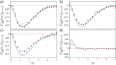
Figure 3: CPF correlation as a function of time for simulated data taking into account different experimental limitations. In all plots the solid blue line represents the ideal theoretical CPF correlation. a), b) and c): V$=1$, V$=0.9$ and V$=0.8$, respectively, for the $\hat{x}$-$\hat{z}$-$\hat{x}$ measurement scheme with $\gamma\tau_{c}=1,$ and initial state $|\uparrow\rangle$, considering infinite (black squares) or finite (red circles) statistics. In d) the red circles are simulated data considering finite statistics for the $\hat{z}$-$\hat{z}$-$\hat{z}$ measurement scheme with initial state $\sqrt{p}|\uparrow\rangle+\sqrt{1-p}|\downarrow\rangle$, $p=0.8$.

As mentioned in the main text, we find experimental issues when going even closer to BMA limit ($\tau_{c}\,\rightarrow\,0$). In Fig. 3d) we show the exact value of the CPF correlation (blue solid curve) and a theoretical simulation including finite statistic effects (red circles) for $\tau_{c}\gamma=0.1$ in the $\hat{z}$-$\hat{z}$-$\hat{z}$ scheme of measurement. In this case, the values of CPF correlation and its “experimental” variations due to fluctuations in the number of counts are comparable. This alone prevents us to assign a non vanishing correlation to memory effects instead of considering it as fluctuations. In this analisis we only took into account finite statistics, making the other experimental issues neglectable.

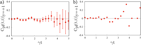
Figure 4: CPF correlation for conditional $y=+1$ in the $\hat{x}$-$\hat{z}$-$\hat{x}$ scheme. $\gamma\tau_{c}=1,$ and $p=1$ are used in this case. a) Experimental data and b) simulation assuming Poissonian fluctuations.

In Fig. 4a), we plot the experimental values of CPF correlation when the outcome of the present (intermediate) measurement is $y=+1.$ In this case, the correlation is null within the error bars, in agreement with what is predicted theoretically. One can see that the error bars increase substantially while time passes. This is related to the fact that the system excitation tends to decay to the reservoir, making the probabilities to find it in an excited state $(y=+1)$ almost null for values of $\gamma t$ larger that 3. In our setup, this is translated as a reduction of the number of coincidence counts, causing the probabilities to be much more sensitive to statistical fluctuations. The fluctuations observed experimentally are compatible with finite count statistics as shown in Fig. 4b), where we plot the result of a simulation assuming Poissonian fluctuations around the ideal theoretical value of the counts.

References

(1) H. P. Breuer and F. Petruccione, The theory of
open quantum systems, (Oxford University Press, 2002).
(2) I. de Vega and D. Alonso, Dynamics of non-Markovian open
quantum systems, Rev. Mod. Phys. 89, 015001 (2017).
(3) H. P. Breuer, E. M. Laine, J. Piilo, and V. Vacchini,
Colloquium: Non-Markovian dynamics in open quantum systems, Rev. Mod. Phys.
88, 021002 (2016).
(4) A. Rivas, S. F. Huelga, and M. B. Plenio, Quantum
non-Markovianity: characterization, quantification and detection, Rep. Prog.
Phys. 77, 094001 (2014).
(5) H. -P. Breuer, E. -M. Laine, and J. Piilo, Measure for the
Degree of Non-Markovian Behavior of Quantum Processes in Open Systems, Phys.
Rev. Lett. 103, 210401 (2009).
(6) E. -M. Laine, J. Piilo, and H. -P. Breuer, Measure
for the non-Markovianity of quantum processes, Phys. Rev. A 81,
062115 (2010).
(7) D. Chruscinski, A, Kossakowski, and A. Rivas, Measures of
non-Markovianity: Divisibility versus backflow of information, Phys. Rev. A
83, 052128 (2011).
(8) C. Addis, G. Brebner, P. Haikka, and S. Maniscalco,
Coherence trapping and information backflow in dephasing qubits, Phys. Rev.
A 89, 024101 (2014).
(9) J. Trapani and M. G. A. Paris, Nondivisibility versus
backflow of information in understanding revivals of quantum correlations
for continuous-variable systems interacting with fluctuating environments,
Phys. Rev. A 93, 042119 (2016).
(10) B. Bylicka, M. Johansson, and A. Acín, Constructive Method
for Detecting the Information Backflow of Non-Markovian Dynamics, Phys. Rev.
Lett. 118, 120501 (2017).
(11) S. Chakraborty, Generalized formalism for information
backflow in assessing Markovianity and its equivalence to divisibility,
Phys. Rev. A 97, 032130 (2018); S. Chakraborty and D. Chruscinski,
Information flow versus divisibility for qubit evolution, Phys. Rev. A
99, 042105 (2019).
(12) G. Guarnieri, C. Uchiyama, and B. Vacchini, Energy
backflow and non-Markovian dynamics, Phys. Rev. A 93, 012118 (2016).
(13) G. Guarnieri, J. Nokkala, R. Schmidt, S. Maniscalco, and B.
Vacchini, Energy backflow in strongly coupled non-Markovian
continuous-variable systems, Phys. Rev. A 94, 062101 (2016).
(14) R. Schmidt, S. Maniscalco, and T. Ala-Nissila, Heat
flux and information backflow in cold environments, Phys. Rev. A 94, 010101(R) (2016).
(15) B. -H. Liu, L. Li, Y. -F. Huang, C. -F. Li, G. -C. Guo, E.
-M. Laine, H. -P. Breuer, and J. Piilo, Experimental control of the
transition from Markovian to non-Markovian dynamics of open quantum systems,
Nat. Phys. 7, 931 (2011).
(16) N. K. Bernardes, A. Cuevas, A. Orieux, C. H. Monken, P. Mataloni,
F. Sciarrino and M. F. Santos, Experimental observation of weak non-Markovianity,
Sci. Rep. 5, 17520 (2015).
(17) N. K. Bernardes, J. P. S. Peterson, R. S. Sarthour, A. M. Souza,
C. H. Monken, I. Roditi, I. S. Oliveira and M. F. Santos,
High Resolution non-Markovianity in NMR, Sci. Rep. 6, 33945 (2016).
(18) D. F. Urrego, J. Flórez, J. Svozilík, M. Nuñez, and A.
Valencia, Controlling non-Markovian dynamics using a light-based structured
environment, Phys. Rev. A 98, 053862 (2018).
(19) S. Yu, Y. -T. Wang, Z. -J. Ke, W. Liu, Y. Meng, Z. -P. Li,
W. -H. Zhang, G. Chen, J. -S. Tang, C. -F. Li, and G. -C. Guo, Experimental
Investigation of Spectra of Dynamical Maps and their Relation to
non-Markovianity, Phys. Rev. Lett. 120, 060406 (2018).
(20) M. Wittemer, G. Clos, H. P. Breuer, U. Warring, and T.
Schaetz, Measurement of quantum memory effects and its fundamental
limitations, Phys. Rev. A 97, 020102(R) (2018).
(21) D. Khurana, B. K. Agarwalla, and T. S. Mahesh,
Experimental emulation of quantum non-Markovian dynamics and coherence
protection in the presence of information backflow, Phys. Rev. A 99, 022107 (2019).
(22) F. A. Pollock, C. Rodríguez-Rosario, T. Frauenheim, M.
Paternostro, and K. Modi, Operational Markov Condition for Quantum
Processes, Phys. Rev. Lett. 120, 040405 (2018); F. A. Pollock, C.
Rodríguez-Rosario, T. Frauenheim, M. Paternostro, and K. Modi, Non-Markovian
quantum processes: Complete framework and efficient characterization, Phys.
Rev. A 97, 012127 (2018).
(23) P. Taranto, F. A. Pollock, S. Milz, M. Tomamichel, and K.
Modi, Quantum Markov Order, Phys. Rev. Lett. 122, 140401 (2019); P.
Taranto, S. Milz, F. A. Pollock, and K. Modi, Structure of quantum
stochastic processes with finite Markov order, Phys. Rev. A 99,
042108 (2019).
(24) A. A. Budini, Quantum Non-Markovian Processes Break
Conditional Past-Future Independence, Phys. Rev. Lett. 121, 240401
(2018); A. A. Budini, Conditional past-future correlation induced by
non-Markovian dephasing reservoirs, Phys. Rev. A 99, 052125 (2019).
(25) S. Yu, A. A. Budini, Y. -T. Wang, Z. -J. Ke, Y. Meng,
W. Liu, Z. -P. Li, Q. Li, Z. -H. Liu, J. -S. Xu, J. -S. Tang, C. -F. Li ,
and G. -C. Guo, Experimental observation of conditional past-future
correlations, Phys. Rev. A 100, 050301(R) (2019).
(26) See the Appendices for detailed derivations and further experimental analysis.
(27) For the conditional we get In fact, when finding the system in the upper state,
the environment must be in the ground state. Therefore, the system evolution
during the first two measurements (interval ) is exactly the same than in
the interval between the second and third measurements (interval ).
Consequently, the CPF correlation vanishes budini .
(28) M. A. Nielsen and I. L. Chuang, Quantum Computation and
Quantum Information (Cambridge University Press, Cambridge, 2000).
(29) F. F. Fanchini, G. Karpat, B. Çakmak, L. K. Castelano, G.
H. Aguilar, O. Jiménez Farías, S. P. Walborn, P. H. Souto Ribeiro, and M. C.
de Oliveira, Non-Markovianity through Accessible Information, Phys. Rev.
Lett. 112,210402 (2014).
(30) O. Jiménez Farías, G. H. Aguilar, A. Valdés-Hernández, P. H.
Souto Ribeiro, L. Davidovich, and S. P. Walborn, Observation of the
Emergence of Multipartite Entanglement Between a Bipartite System and its
Environment, Phys. Rev. Lett. 109, 150403 (2012).
(31) P. G. Kwiat, E. Waks, A. G. White, I. Appelbaum, P. H.
Eberhard, Ultrabright source of polarization-entangled photons, Phys. Rev.
A. 60, 773(R) (1999).
(32) M. Bonifacio and A. A. Budini (unpublished).