Efficient Simulation of Sparse Graphs of Point Processes

Abstract.

We derive new discrete event simulation algorithms for marked time point processes. The main idea is to couple a special structure, namely the associated local independence graph, as defined by Didelez (didelez), with the activity tracking algorithm (cise-muzy) for achieving high performance asynchronous simulations. With respect to classical algorithm, this allows reducing drastically the computational complexity, especially when the graph is sparse.

1. Introduction

Point processes in time are stochastic objects that model efficiently event occurrences. The variety of applications is huge: from medical data applications (time of death or illnesses) to social sciences (dates of crimes, weddings, etc), from seismology (earthquake occurrences) to micro-finance (actions of selling or buying a certain assets), from genomics (gene positions on the DNA strand) to reliability analysis (breakdowns of complex systems) (see e.g. (andersen; didelez; Hoff; VeO82; RBS; cha)).

Most of the time, point processes are multivariate, in the sense that either several processes are considered at the same time, or in the sense that one process regroups together all the events of the different processes and marks them by their type. A typical example consists in considering either two processes, one counting the wedding events of a given person and one counting the birth dates of children of the same person. One can see this as a marked process which regroups all the possible dates of birth or weddings independently and on each event one marks it by its type, here wedding or birth.

In the sequel, we denote the individual process $N_{j}$, the set of all events corresponding to type $j$, for $j=1,...,M$ and the joint process $N=N_{1}\cup..\cup N_{m}$. In this multivariate or marked case, the individual processes are usually globally dependent, the apparition of one event or point on a given type influencing the apparition of other points for the other types and the simulation of the whole system cannot be easily parallelized.

This is especially true in neuroscience (IEEE). Let us detail a bit more this set up which is a benchmark example here. Neurons are excitable electric cells that are linked together inside a huge network ($10^{11}$ for humans (nbNeurons), $10^{8}$ for rats (Herculano-Houzel2518), $10^{6}$ for coackroaches), each cell receives inputs from approximately $10^{3}$ to $10^{4}$ presynaptic (upstream) neurons (PAKKENBERG200395). Depending on its excitation, the neuron might then produce an action potential also called spike, information which is propagated to postsynaptic (downstream) neurons.

From a stochastic point of view, one might then see the spike trains emitted by a given neuron as an individual point process which in fact is embedded in a multivariate point process with $M$, the total number of neurons as the total number of types. The size of the network requires then very well adapted simulation schemes that may use the relative sparseness of the network with respect to the global size of the network.

To do so, we use the mathematical notion of local independence graph for marked point processes due to Didelez (didelez), which is detailed in Section 4 and which informally corresponds to the real neuronal network. In this sense, in the sequel we call marks, processes and type the nodes of the graph. The only strong assumption that is used is the time asynchrony hypothesis, (i.e. points or events of different mark or types, meanings points or events appearing in different nodes, cannot occur at the exact same time) together with the fact that all processes have a conditional intensity (bremaud1981point).

Simulation of point processes has a long history that dates back to Doob in the 40’s (Doob) for Markov processes. In the 70’s, Gillespie (gillespie) popularized the method for a particular application: chemical reactions. At the same time, Lewis and Shedler (lewis) proposed a thinning algorithm for simulating univariate inhomogeneous Poisson processes (this can also be viewed as a rejection method). Few years later, Ogata (ogata) produced a hybrid algorithm able to simulate multivariate point processes in the general case even if they are not markovian, including both a choice of the next point by thinning and a choice of the node to activate thanks to Gillespie principle. This method is still up to now the benchmark for simulating such processes, and is for instance used in recent packages such as ppstat in R (2012). It has been rediscovered many times in various cases, most of the time as a Generalized Gillespie method (see for instance (barrio)).

When the number of types or nodes is huge, this method can quickly become inefficient in terms of computational times. Many people have found shortcuts, especially in Markovian settings. For instance, Peters and de With (peters) proposed a new simulation scheme exploiting a network of interaction for particular physical applications. In (doucet), the authors reformulated this algorithm in a more mathematical way for a particular case of Piecewise Deterministic Markov Processes. People have even exploited very particular structures such as Hawkes processes, with exponential interactions (special case which leads to Markovian intensities) (dassios), to be able to simulate huge networks, as in the Python package tick (2017).

In the mean time, the technique of discrete event simulation first appeared in the mid-1950s (tocher) and was used to simulate the components (machines) of a system changing state only at discrete “events”. This technique has then been formalised in the mid-1970s (tms76). Discrete event modelling and simulation seem very close to point process models (dealing with events, directed graphs, continuous time, etc.). Against all expectations, as far as we know, there is no direct use of any discrete event simulation algorithm for point processes. Maybe, the sophistication of these algorithms being of the same order than the mathematical technicality of point processes, prevented any direct application. Besides, the continuous nature of the conditional intensity associated to a point process with respect to the discreteness of event-based simulations could make appear the two domains as separated whereas discrete event theory is a computational specification of mathematical (continuous) systems theory (mesarovic) integrating more and more formally stochastic simulation concepts (tms2). We hope to show here that both domains can take advantage from each other, by introducing new discrete-events models that act as generators of point processes. Especially, whereas discrete event simulation algorithms have been developed considering independently the components (nodes) of a system, a new algorithm for activity tracking simulation (cise-muzy) have been proposed to track activity (events from active nodes to children). The activity tracking algorithm is used here and proved to be the right tool for both simplifying usual discrete event algorithms (which are difficult to relate to usual point process algorithms) and efficiently simulating point processes.

Our aim is to derive a new simulation algorithm, which generalises the algorithm of (doucet) to general multivariate point processes that are not necessarily Markovian, by exploiting the underlying network between the types, which is here a local independence graph. In Section 2, the main mathematical background and notations are provided and the classical multivariate algorithm due to Ogata (ogata) is explained. A simplified version in discrete event terms and called full scan algorithm is proposed. In Section 3, discrete event data structure and operations specific to point processes are designed. In Section 4, after recalling the notion of local independence graph (didelez), a new local graph algorithm is presented. In Section 5, we evaluate the computational complexities of both algorithms on Hawkes processes with piecewise constant interactions, which model easily neuronal spike trains (IEEE). We show that in this case, for sparse graphs, new local graph algorithm clearly outperforms the classical Ogata’s algorithm in its discrete event version.

2. Set-up

2.1. Mathematical framework

A (univariate) point process $N$ in $\mathbb{R}_{+}$ is a random countable set of points of $\mathbb{R}_{+}$. For any subset $A$ of $\mathbb{R}_{+}$, $N(A)$ is the number of points that lie in $A$.

As real random variables might be defined by their density with respect to Lebesgue measure, if it exists, a point process is characterised by its conditional intensity with respect to a given filtration or history $(\mathcal{F}_{t},t\geq 0)$. For the mathematical details, we refer the reader to (bremaud1981point). Informally, the filtration or history at time $t-$, $\mathcal{F}_{t-}$, contains all the information that is needed to simulate the next point of $N$, when one is just before time $t$. It usually includes as generators, all the points $T\in N$ such that $T<t$ in particular. The (conditional) intensity of the point process $N$ is then informally defined  (bremaud1981point) by

$$\lambda(t)=\lim_{dt\to 0}\frac{1}{dt}\mathbb{P}\left(\mbox{there is a point of }N\mbox{ in }[t,t+dt]\Big{|}\mathcal{F}_{t-}\right),$$

for infinitesimal $dt$, where $\mathbb{P}\left(\mbox{there is a point of }N\mbox{ in }[t,t+dt]\Big{|}\mathcal{F}_{t-}\right)$ is the probability that a point appears in the interval $[t,t+dt]$ given what happened strictly before $t$ in the history. This is a random process which, at time $t$, may depend in particular on all the past occurrences of the process itself, that is the $T<t$.

A multivariate point process can be seen as a collection of $M$ different point processes $N_{j}$. With the time asynchrony hypothesis, one can also consider equivalently the univariate joint point process $N=N_{1}\cup...\cup N_{M}$ and say that for each point $t$ of $N$ there is one and only one subprocess $j$ such that $t\in N_{j}$. This $j$ is then called the mark of point $t$, or the node associated to $t$.

We are given the set of intensities of each of the $N_{j}$, $t\mapsto\lambda_{j}(t)$, with respect to a common filtration $(\mathcal{F}_{t},t\geq 0)$. Note that $\mathcal{F}_{t-}$ includes as generators, all the points $T\in N$, the joint process such that $T<t$ as well as their respective marks.

Examples

Let us give just few basic examples

• Homogeneous Poisson processes with rates $(\nu_{i})_{i=1,...,M}$. In this case, all $\lambda_{i}$ are constant and not even random and for all $i$,

  $$\lambda_{i}(t)=\nu_{i}.$$

  We see in this expression, that the intensities do not depend neither on time, nor on the previous occurrences. This is why one often refers to such dynamics as “memoryless”. Since these processes do not interact, one can of course simulate each $N_{i}$ in parallel if need be. In this case, for each of them, it is sufficient to simulate the time elapsed until the next point, by an exponential variable of parameter $\nu_{i}$, independently from anything else. To unify frameworks, this exponential variable might also be seen as $-\log(U)/\nu_{i}$, with $U$ a uniform variable on $[0,1]$.

• Inhomogeneous Poisson processes with time-dependent rates $(f_{i})_{i=1,...,M}$. In this case, the $\lambda_{i}$’s are not necessarily constant and but they are still non random and for all $i$,

  $$\lambda_{i}(t)=f_{i}(t).$$

  Once again parallelization is possible, and for each individual process $N_{i}$ and given point $t_{k}^{i}$, one finds the next point $t_{k+1}^{i}$ by solving

  $$\int_{t_{k}^{i}}^{t_{k+1}^{i}}f_{j}(s)\mathop{}\,\mathrm{d}s=-\log(U)$$

• Linear multivariate Hawkes process with spontaneous parameter $(\nu_{j})_{j=1,...,M}$ and non negative interaction functions $(h_{j\to i})_{i,j=1,...,M}$ on $\mathbb{R}_{+}$. This process has intensity

  (1) $$\lambda_{i}(t)=\nu_{i}+\sum_{j=1}^{M}\sum_{T\in N_{j},T<t}h_{j\to i}(t-T).$$

  This process is used for many excitatory systems, especially the ones modelling the spiking activity of neurons (IEEE). It can be interpreted in this sense, informally: to a homogeneous Poisson process of rate $\nu_{i}$, which models the spontaneous activity of the neuron $i$, one adds extra-points coming from the interactions. Typically a point $T$ of mark (neuron) $j$ adds a term $h_{j\to i}(\delta)$, after delay $\delta$ to the intensity of $N_{i}$ making the apparition of a new point at time $t=T+\delta$ more likely. In this sense there is an excitation of $j$ on $i$. Here we see a prototypical example of global dependence between the marks. Each new point for each mark depends on all the points that have appeared before, with all the possible marks, preventing a brute force parallelization of the simulation. Except when the $h_{j\to i}$’s are exponentially decreasing (dassios), this process is clearly not Markovian. It is for this kind of general process that one needs efficient simulation algorithms.

2.2. Simulation of univariate processes

The time-rescaling theorem (see (brown) or (bremaud1981point) for more mathematical insight) states that if a point process $N$ has a conditional intensity $\lambda(t)$, and if

$$\forall t,\Lambda(t)=\int_{0}^{t}\lambda(s)\mathop{}\,\mathrm{d}s,$$

then $\mathcal{N}=\{\Lambda(T),T\in N\}$ is a Poisson process of rate 1. This is why, even for general point processes, it is always possible to find, by iteration the next point of $N$ by solving recursively, for all $k\in\mathbb{N}^{*}$ the set of positive natural numbers,

(2) $$\int_{t_{k}}^{t_{k+1}}\lambda(s)\mathop{}\,\mathrm{d}s=-\log(U)$$

initializing the method with $t_{0}=0$.

Of course, to be able to mathematically solve this easily, one needs to be able at time $t_{k}$ to compute $\lambda(t)$ on $(t_{k},+\infty)$ if no other point occurs. This in particular happens if the filtration $\mathcal{F}_{t}$ is reduced to the filtration generated by the points themselves and this is what we will assume here. Of course all algorithms discussed here can easily be adapted to richer filtrations, as long as the computation of $\lambda(t)$ on $(t_{k},+\infty)$ can be carried out (if no other point occurs).

In this situation, two cases might happen, each of them leading to a different algorithm:

Transformation method::

The function $\lambda(t)$ on $(t_{k},+\infty)$ (and if no other point occurs) has an easily computable primitive function with inverse $\Lambda^{-1}(t)$. Then (2) reduces to

$$t_{k+1}=\Lambda^{-1}(-\log(U)+\Lambda(t_{k})).$$

Thinning method::

It applies if the previous computation is not possible or easy but one can still compute $\lambda^{*}(t)\geq\lambda(t)$ such that $\lambda^{*}(t)$ has all the desired properties of the transformation method (typically $\lambda^{*}(t)$ is constant, with constant that might depend on the $t_{\ell}$ for $\ell\leq k$). Then the algorithm does as follows to compute a possible next point (cf. Algorithm 1). If thinning for Poisson processes is due to (lewis), it has been generalized to general processes by Ogata (ogata). One can find a complete proof in (maria).

1:initialize $t_{0}^{*}\leftarrow t_{k}$

2:repeat

3:     Generate next point $t^{*}$ after $t_{0}^{*}$ of a point process with intensity function $\lambda^{*}$ by the Transformation method.

4:     Generate $U\sim\mathcal{U}[0,1]$

5:     if $U>\lambda(t^{*})/\lambda^{*}(t^{*})$ then # Rejection

6:         $t_{0}^{*}\leftarrow t^{*}$      

7:until $U\leq\lambda(t^{*})/\lambda^{*}(t^{*})$

8:return $t_{k+1}\leftarrow t^{*}$

Algorithm 1 Thinning algorithm

2.3. Discrete event version of classical multivariate algorithm for point processes

To simulate multivariate processes, Ogata (ogata) made an hybridation between two different notions : the thinning algorithm presented above and the attribution of marks. Indeed, since all processes $N_{j}$ are communicating with each other, Ogata’s idea for the attribution of marks is to generate the next point of the aggregated process $N$ and, then, to decide for its mark.

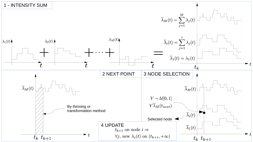
In the present article, we choose to discard the thinning part, which can be added to all the algorithms that we derive here. The attribution part of Ogata’s multivariate algorithm (ogata), is referred in the sequel as full scan, because the intensities of all nodes of the graph need to be scanned and updated at each time stamp $t_{k}$. Once the next point of $N$ is decided, the basic idea for the attribution of marks is to attribute them at random, the distribution taking into account the relative value of the intensity of each subprocess. The main steps of this algorithm are presented in Figure 1 for a visual representation of the method. More details about the algorithm steps are provided through the Hawkes application in Section 5.

1:$t_{0}\leftarrow 0$

2:while $t_{k}<T$ do

3:     Compute intensity sums $\sum_{j=1}^{i}\lambda_{j}(t)=\overline{\lambda}_{i}(t)$, for $i\in\{1,...,M\}$ on $t\in(t_{k},+\infty)$

4:     Get by simulation $t_{k+1}$ as the next point of a univariate point process of intensity $\overline{\lambda}_{M}(t)$

5:     Select the unique possible node $i_{k+1}$, such that $\frac{\overline{\lambda}_{i_{k+1}-1}(t_{k+1})}{\overline{\lambda}_{M}(t_{k+1})}<V\leq\frac{\overline{\lambda}_{i_{k+1}}(t_{k+1})}{\overline{\lambda}_{M}(t_{k+1})}$, with $V\sim\mathcal{U}[0,1]$ and $\overline{\lambda}_{0}=0$

6:     Update intensities $\lambda_{j}$ on $(t_{k+1},+\infty),\forall j\in\{1,...,M\}$

7:     $k\leftarrow k+1$

8:return points $(t_{1},...,t_{k-1})$ and associated nodes $(i_{1},...,i_{k-1})$

Algorithm 2 Full scan multivariate algorithm modified from (ogata)

Figure 1. Steps of the full scan algorithm for point processes. The intensities are piecewise constant (cf. Section 5).

Original Ogata’s algorithm uses thinning at step 4 of Algorithm 2. However the complexity of a thinning step is difficult to evaluate because it depends on both the complexity of the upper-bounding function $\lambda^{*}$ and how far this function is from $\lambda$, which influences how much time the thinning algorithm rejects. Therefore for a clear evaluation of the complexity, we focused on simulations where the transformation method is doable, typically when the intensities are piecewise constant.

3. Specific discrete event data structures and operations

Before introducing our new algorithm, we present a particular structure, which is very important for discrete events algorithm : the scheduler.

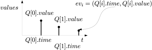
A scheduler $Q$ is a data structure, which can be represented as an ordered set of events, and which is provided with a set of operations for ensuring the correct order of the events. The events are noted $ev_{i}=(t_{i},v_{i})$, where $t_{i}$ is the event time and $v_{i}$ is the event value. The events in the scheduler are increasingly ordered in time, i.e., $ev_{i},ev_{j}\in Q$, $ev_{i}<ev_{j}\iff t_{i}<t_{j}$. The length of the scheduler is noted $|Q|$.

Figure 2. Example of events in scheduler $Q$. For an event $ev_{i}$ in the scheduler, the value is accessed by $Q[i].value$ and the time is accessed by $Q[i].time$, with $i=0$ the first event index.

In both full scan and local graph algorithms schedulers are used. They are usually implemented using one of the many kinds of self-balancing binary tree. The choice of structure (AVL, red-black, etc.) depends on corresponding operation complexity. Here we choose the red-black self balancing tree, which exhibits the best performance with respect to other usual self-balancing trees (heger).

To make a scheduler, the red-black tree is equipped with a set of classical (insert, remove, upper bound and lower bound) and non-classical operations. All these operations, except stated otherwise, have time complexity bounded by the logarithm $\log_{2}$ of the number of elements in the set. In addition it is supposed that any element of the scheduler can be accessed with a constant time. This may not be the case depending on the language used for the implementation. However, it is true for C++ language, which was used in our implementation.

3.1. Basic scheduler operations

We describe and illustrate the set of operations completing the red-black tree to form the scheduler data structure needed for our algorithms. Any operation on a scheduler $Q$ directly modifies it. Also, to simplify the operations, it is supposed that all events stored in a scheduler $Q$ are unique.

Access element operation:

$(t^{i},v^{i})_{i\in\{0,\dots,|Q|-1\}}$ is the list of events stored in scheduler $Q$ and sorted by ascending values of $t$. Then operation $Q[i]$ returns event $(t^{i},v^{i})$ with constant time complexity $\mathscr{O}(1)$.

Insert operation:

of an event $(t,v)\in\mathbb{R}_{+}\times\mathbb{R}$ (cf. Figure 3): $Q\oplus(t,v)$ inserts the event in the tree. This operation has a total maximum complexity of $\mathcal{O}(log_{2}(|Q|))$, to find the place of the event and rebalance the tree.

Figure 3. A graphical example of the insertion of a new event $(t_{*},v_{*})$ inside a scheduler. There are two cases: if the event time is unmatched in the set of event times already present in the scheduler (case $t_{1}<t_{*}<t_{2}$), the event is just inserted in the right place; otherwise (case $t=t_{*}$) the event in the scheduler with the same time has its value increased by the value $v_{*}$ of the new event.

Remove operation:

of an event (cf. Figure 4): $Q\ominus(t,v)$, removes the event $(t,v)$ from the tree. This operation has a maximum complexity of $\mathscr{O}\left(\log_{2}(|Q|)\right)$, to find the place of the event and rebalance the tree. If the index $i$ of the element is known, the remove operation can be executed in constant time.

Figure 4. A graphical example of the removal of an event given its time $t$.

Remove first operation:

$Q^{*}$ over the scheduler $Q$, which removes the first event $Q[0]=(t^{0},v^{0})$ from the scheduler, the second event becoming the first. Operation $\cdot^{*}$ has complexity $\mathcal{O}(1)$.

Prune operation:

of the scheduler $Q^{t}$ (cf. Figure 5) removes all events $(t^{*},v^{*})$ from $|Q|$ whose time value $t^{*}\leq t$. The operation $Q^{t}$ has complexity $\mathcal{O}\left(log_{2}(|Q|)+|\textrm{number of events until time }t|\right)$.

Figure 5. A graphical example of the prune operation : Here all the points with a time less or equal to $t$ (here the first two points of this scheduler) are removed. The time complexity of the operation is $\mathscr{O}(\log_{2}(4)+2)$ (scheduler of size $|Q|=4$ and $2$ events removed).

Upper and lower bound operations:

(cf. Figure 6): Upper bound operation: $\left\lceil t\right\rceil_{Q}$ and lower bound operation $\left\lfloor t\right\rfloor_{Q}$, return the smaller event $(t^{*},v^{*})$ verifying respectively $t^{*}>t$ and $t^{*}\geq t$. In both cases the time complexity of the operation is $\mathcal{O}(log_{2}(|Q|))$.

Figure 6. Upper/lower bound operations on an example of scheduler $Q$. For $t_{k}<t<t_{\ell}$ the upper bound operation consists of $\left\lceil t\right\rceil_{Q}=\ell$. The lower bound operation consists of $\left\lfloor t\right\rfloor_{Q}=k$.

3.2. Using a scheduler to represent piecewise constant functions

Let $h\colon\mathbb{R}^{*}\to\mathbb{R},t\mapsto h(t)$ be a piecewise constant function with finite support $S\subseteq\mathbb{R}^{*}$. A scheduler can encode piecewise constant functions on $S$. There are two possible methods to achieve this:

1. Let each discontinuity $(t,h(t))$ be its own event in the scheduler $Q$ representing the function $h$ (see top part of Figure 7).

2. Represent the discontinuity not as a new value $(t,h(t))$ but as an increment, that is a difference between the new value of $h$ after the discontinuity and the value of $h$ just before: $(t,h(t)-h(t_{-}))$ (see bottom part of Figure 7).

The first representation is more straightforward, and is very efficient when the function is stored only for lookups: the function can then be stored in an array and a dichotomic search algorithm be used to locate any event in logarithmic time.

However, if discontinuities must be introduced or removed, for instance by adding another piecewise constant function to $h$, then some of the events stored in the scheduler may need to be changed or moved in the scheduler, thus creating an undesirable overhead. For instance in the first line of figure 7, a piecewise function $h$ (first column) is represented and encoded (second column) with the straightforward method by a scheduler. Last column shows the new encoding representing a sum. The discontinuity at $t_{k+2}$ had to be modified because of the introduction of discontinuities at $t_{k+3}$ and $t_{k+4}$. For a function with many more discontinuities, or when summing two piecewise functions of similar size, the operation would necessitate to modify a large part of the already represented points.

The solution we proposed is to store not the values $h(t)$ of the function $h$ at a time $t$ where a discontinuity happens, but the variation $\Delta h_{t}=h(t)-h(t_{-})$ of the value of $h$ during the discontinuity. An example is represented on the second line of Figure 7.

Function	Encoding	Summing

Figure 7. Example of a straightforward encoding of a piecewise constant function (first line) and an optimised one (second line). We use the notation $H_{n}=h(t_{k+n}),n\in\mathbb{N}$ for concision. The Function column represents the piecewise constant function $h$ to encode (plain lines), as well as another function $h^{\prime}$ (dashed lines, see column Summing). Column Encoding represents in bold the events $(t_{n},h(t_{n}))$ encoded by a scheduler representing the function $h$. Column Summing represents in bold the values encoded by a scheduler now representing the function $h+h^{\prime}$.

Let us now present two different operations for piecewise contant functions with this encoding:

Piecewise sum,:

which is in fact a union operation over two schedulers $Q,Q^{\prime}$ encoding two piecewise constant functions (cf. Figure 8): The operation $Q\cup Q^{\prime}$ has complexity $\mathcal{O}(min(|Q|,|Q^{\prime}|)log_{2}(max(|Q|,|Q^{\prime}|)))$, since the smallest scheduler is inserted into the largest scheduler.

Piecewise prune operation:

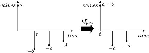
of the scheduler $Q^{t}_{pcw}$ (cf. Figure 9): removes from scheduler $Q$ all the events $(t^{*},v^{*})$ with $t^{*}\leq t$, while accumulating all the values $v^{*}$ up to time $t$. At the end of the operation the scheduler begins with an event of the form $(t,\sum v^{*})$. The operation $Q^{t}_{pcw}$ has complexity $\mathcal{O}(log_{2}(|Q|)+|\textrm{number of events until time }t|)$.

Shift operation:

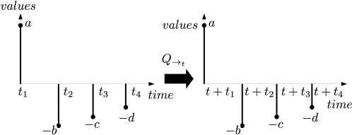
of the scheduler $Q_{\rightarrow_{t}}$ (cf. Figure 10): shifts all points by $t$. The operation $Q_{\rightarrow_{t}}$ has complexity $\mathcal{O}(|Q|)$.

Figure 8. A graphical example of the union of two schedulers. The events of $\text{Sched}_{i}$ are represented as dotted, while the events of $\text{Sched}_{j}$ are dashed. In the merged scheduler $\text{Sched}_{k}$, the values of events at the same time in both schedulers $i$ and $j$ are summed and the resulting event is represented with a continuous line.

Figure 9. Example of piecewise prune operation $Q^{t}_{pcw}$.

Figure 10. The shift operation $Q_{\rightarrow_{t}}$

4. Local graph algorithm for point processes

4.1. Local independence graph

Local independence graphs are fully presented in a sound mathematical form in (didelez). For a given multivariate point process $N_{j},{j=1,...,M}$, the corresponding local independence graph is a directed graph on the nodes $j=1,...,M$ (see for instance Figure 11). We assume for sake of simplicity that the filtration is reduced to the internal history, that is $\mathcal{F}_{t}$ is generated only by the $T<t$ in $N=N_{1}\cup...\cup N_{M}$ and their associated mark or node.

To explain more fully what a local independence graph means, we need to define rougher filtration. For a subset $I\subset\{1,...,M\}$, $\mathcal{F}_{t}^{I}$ is the filtration generated by the $T<t$ in $\cup_{i\in I}N_{i}$ and their associated node.

In a local independence graph, the absence of edge $j\to i$ means that the apparition of a point at time $t$ in $N_{i}$ is independent from $\mathcal{F}_{t-}^{\{j\}}$ conditionally to $\mathcal{F}_{t-}^{\{j\}^{c}}$, where $\{j\}^{c}=\{1,...,M\}\setminus\{j\}$.

So this means that for every time $t$, the intensity $\lambda_{i}(t)$ of $N_{i}$ does not depend directly on the positions of the points of $N_{j}$ strictly before $t$.

This extends directly to the notion of parents and children in the graph. For a given node $i$, one defines

$$pa(i)=\{j,j\to i\mbox{ is in the graph}\}\mbox{ and }ch(i)=\{j,i\to j\mbox{ is in the graph}\}.$$

Therefore it means that the intensity $\lambda_{i}(t)$ at time $t$ of $N_{i}$ in fact only depends on the points of $N_{j}$ for $j\in pa(i)$ strictly before $t$.

Conversely, a point on $N_{i}$ directly impacts the occurrence of points for $N_{j}$ for $j\in ch(i)$. Note that in any case, it also impacts the next point of $N_{i}$ because even for a Poisson process without memory one needs by the transformation method to know $t_{k}$ for finding $t_{k+1}$. However, it will not have any direct impact on the future points of $N_{j}$ for $j\not\in ch(i)\cup\{i\}$.

Figure 11. Example of local independence graph. With this graph, $ch(2)=\{3,6\}$ and $pa(2)=\{1,5\}$. As indicated by the difference of colour, a point with mark $2$ shall impact the point generation only for $\{2\}\cup\{3,6\}$.

For instance, for linear Hawkes process (cf. Equation 1), $ch(i)=\{j/h_{i\to j}\neq 0\}.$

4.2. Local-graph algorithm

The children of each node are stored in a simple one dimensional array, whose indexes are the node indexes, and whose cells contain vectors of the children indexes. So accessing a node simply costs $\mathcal{O}(1)$.

Because of the interpretation of $I=ch(i)\cup\{i\}$ of a given node $i$ given above in the local independence graph, it means that in fact, after having simulated $t_{k}$ with mark/node $i_{k}$ in the joint process, we know that only the next points of $N_{j}$ for $j\in I$ have to be modified.

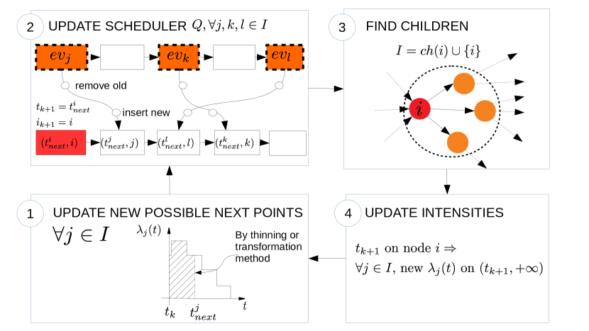
At simulation level, discrete events are used to track activity nodes associated to selected points (time stamps) to their children. Discrete events are stored into a scheduler $Q$ of events $ev_{i}=(t_{next}^{i},i)$, where $t_{next}^{i}$ is the possible next point associated to node $i$.

The local graph algorithm for point processes is described in Algorithm 3. A visual representation is presented in Figure 12.

Let us detail a bit more each step.

• At Step a/, we decide for the next possible point of each of the subprocesses $N_{i}$ by either using the transformation method or the thinning algorithm (Algorithm 1).

• At Step b/, for each $i\in I$ we remove the old event associated to $i$ and insert the one computed at Step a/.

• At Step c/, we retrieve the minimum of all possible times to find out which subprocess $i$ is actually generating a new point.

• At Step d/, we look for the children of $i$ and update $I$.

• Step e/ depends hugely on the type of process at hand. The apparition of a new point has clear impact on the intensity but this depends on the formula. For instance if the intensity is given by Equation (1), we need to shift intensities and update sums (see Section 5 for more details).

More details about the algorithm steps are provided in Section 5, which presents in full details the application of the algorithm to the Hawkes case.

1:$k\leftarrow 0,t_{k}\leftarrow 0$

2:$I\leftarrow\{1,...,M\}$

3:while $t_{k}<T$ do

4:     Compute the next possible points $t^{i}_{next}$ for each $i\in I$ based on intensity $\lambda_{i}$ on $(t_{k},+\infty)$

5:     Update $Q$ with each next possible point $t^{i}_{next}$ for each $i\in I$

6:     Get next selected point $t_{k+1}\leftarrow min\{t^{i}_{next}\}$ and $i$ the associated node, updating $Q\leftarrow Q^{*}$

7:     Find the children of $i$ and update $\bm{I}\leftarrow ch(i)\cup\{i\}$

8:     Update intensities $\lambda_{j}(t)$ for each node $j\in I$ on $(t_{k+1},+\infty)$

9:     $k\leftarrow k+1$

10:return $(t_{1},...,t_{k-1})$ points and associated nodes $(i_{1},...,i_{k-1})$

Algorithm 3 Local graph algorithm for the simulation of point processes: Application of the simulation activity tracking algorithm (cise-muzy).

Figure 12. Steps of the local graph algorithm for the simulation of point processes. As for figure 1, the intensities are piecewise constant.

5. Hawkes evaluation

We want to evaluate the complexity of the previous algorithms, but this of course depends on the computational complexity of the conditional intensities associated to each point process. Previous general algorithms for simulating point processes are applied here to non explosive Hawkes processes with piecewise constant interactions with finite support (see Equation (1)). In this situation, note that the $\lambda_{i}$’s become piecewise constant, so that the complexity for calculating such intensities or updating them will be linked to the number of breakpoints of the corresponding piecewise constant function. Moreover with piecewise constant intensities, one can apply the transformation method directly, so we do not evaluate the complexity of the thinning /rejection step. The general algorithms are specified at data structure level in order to detail the computational complexity of each algorithmic step.

5.1. Notation and data structures

In the following, $\leftrightarrow$ means ”corresponds to the mathematical notation”. Data structure notation consists of:

• $Q$: A scheduler of next point events $ev_{i}=(t_{next}^{i},i)$, where $t_{next}^{i}$ is a possible next point associated to node $i$.

• $L[i](\leftrightarrow\lambda_{i})$: is the scheduler corresponding to the piecewise constant intensity of node $i$, The length of the scheduler is $L_{t}^{i}=length(L[i])$ when $L[i][0].time=t$.

• $h[j][i](\leftrightarrow h_{j\rightarrow i})$: is the scheduler corresponding to the piecewise constant interaction $h_{j\rightarrow i}$ (with support included in $[0,S]$) from node $j$ to node $i$. The maximum number of events in $h[j][i]$ is noted $A\geq length(h[j][i])$.

• $\overline{L}=L[1]\cup...\cup L[M]$ ($\leftrightarrow\overline{\lambda}(t)=\sum_{i=1}^{M}\lambda_{i}(t)$): is a scheduler storing the piecewise sum of all $L[i]$, from node $1$ to node $M$ (cf. Figure 8).

• $\overline{L}[i]=L[1]\cup...\cup L[i]$ ($\leftrightarrow\overline{\lambda}_{i}(t)=\sum_{j=1}^{i}\lambda_{j}(t)$): is a scheduler storing the partial piecewise sum of the intensities from node $1$ to node $i$. Obviously, $\overline{L}[M]=\overline{L}$.

5.2. Algorithm for the transformation method for piecewise constant intensities

Algorithm 4 presents the basic transformation method for piecewise constant conditional intensity functions, here represented by the scheduler $Q$ (cf. Equation 2).

1:function getTnext($Q$)

2:     $V\sim\mathcal{U}[0,1]$

3:     $integral\leftarrow 0$

4:     $t_{next}\leftarrow Q[0].time$

5:     $k\leftarrow 0$

6:     $val\leftarrow 0$

7:     repeat

8:         $val\leftarrow val+Q[k].value$

9:         $integral\leftarrow integral+(Q[k+1].time-Q[k].time)\times val$

10:         $k\leftarrow k+1$

11:     until $(integral>-log(V)\text{ or }k=size(Q)-1)$

12:     if $integral\leq-log(V)$ then

13:         $val\leftarrow val+Q[k].value$      

14:     return $t_{next}\leftarrow Q[k].time-\frac{integral+log(V)}{val}$ // $t_{next}\leftarrow+\infty$ if $val=0$

Algorithm 4 Function getTnext(Q) with $Q$ a scheduler storing the events corresponding to a piecewise constant intensity trajectory.

The complexity of the getTnext(Q) operation is $\mathcal{O}(|Q|)$.

5.3. Full scan and local graph algorithms

Algorithm LABEL:alg:centH is the application of Algorithm 2 to Hawkes processes. The mention to a, b c, d refers to the steps in Algorithm 2. We split step d to lower the complexity. The value $T$ is an arbitrary stopping time, the condition $t_{k}<T$ ending the main loop in both Algorithm LABEL:alg:centH and Algorithm LABEL:alg:distributedH can be changed by whatever condition is deemed more appropriate by the modeller.

1:$t_{0}\leftarrow 0$

2:$k\leftarrow 0$

3:while $t_{k}<T$ do

4:     $\overline{L}[1]\leftarrow L[1]$

5:     for all $j\in\{2,...,M\}$ do