Tempered Lefschetz thimble method and its application to the Hubbard model away from half filling

Abstract:

The tempered Lefschetz thimble method (TLTM) is a parallel-tempering algorithm towards solving the numerical sign problem. It tames both the sign and ergodicity problems simultaneously by tempering the system with the flow time of continuous deformations of the integration region. In this article, after reviewing the basics of the TLTM, we explain a new algorithm within the TLTM that enables us to estimate the expectation values precisely with a criterion ensuring global equilibrium and the sufficiency of the sample size. To demonstrate the effectiveness of the algorithm, we apply the TLTM to the quantum Monte Carlo simulation of the Hubbard model away from half filling on a two-dimensional lattice of small size, and show that the obtained numerical results agree nicely with exact values.

1 Introduction

The sign problem is one of the major obstacles for numerical calculations in various fields of physics, including finite density QCD [1], quantum Monte Carlo (QMC) calculations of quantum statistical systems [2], and the numerical simulations of real-time quantum field theories. In this article, we argue that a new algorithm which we call the “tempered Lefschetz thimble method” (TLTM) [3, 4] is a promising method towards solving the sign problem. We exemplify its effectiveness by applying the method to the QMC simulations of the Hubbard model away from half filling on a two-dimensional lattice of small size (see [4] for a detailed analysis).

2 Sign problem and the (generalized) Lefschetz thimble method

We start with reviewing Lefschetz thimble methods [5, 6, 7, 8, 9, 3, 10, 4].

Let ${\mathbb{R}}^{N}=\{x\}$ be a configuration space of $N$-dimensional real variable $x=(x^{i})$ $(i=1,\ldots,N)$, and $S(x)$ the action. Our main concern is to estimate the expectation value of an observable $\mathcal{O}(x)$,

$$\langle\mathcal{O}(x)\rangle_{S}\equiv\frac{\int dx\,e^{-S(x)}\,\mathcal{O}(x)}{\int dx\,e^{-S(x)}}.$$ (1)

When $S(x)$ takes complex values ($S(x)=S_{R}(x)+i\,S_{I}(x)$), one can no longer regard the Boltzmann weight $e^{-S(x)}/\int dx\,e^{-S(x)}$ as a probability distribution function, and thus a direct use of MCMC method to estimate (1) is invalidated. An obvious workaround is the reweighting with $S_{R}(x)$:

$$\langle\mathcal{O}(x)\rangle_{S}=\frac{\langle e^{-i\,S_{I}(x)}\,\mathcal{O}(x)\rangle_{S_{R}}}{\langle e^{-i\,S_{I}(x)}\rangle_{S_{R}}}.$$ (2)

However, in MCMC simulations, the numerator and the denominator are estimated separately, and for large $N$ (or in general, when the action takes large values) the integrals of the numerator and the denominator may become highly oscillatory and take vanishingly small values of $e^{-O(N)}$. Then, the estimate of (2) with a sample of size $N_{\rm conf}$ will take the following form:

$$\langle\mathcal{O}(x)\rangle_{S}\approx\frac{e^{-O(N)}+O(1/\sqrt{N_{\rm conf}})}{e^{-O(N)}+O(1/\sqrt{N_{\rm conf}})}.$$ (3)

This means that we need to set the sample size to be exponentially large, $N_{\rm conf}=e^{O(N)}$, in order to make an estimation with relatively small statistical errors. This is the sign problem.

In this article, we always assume that both $e^{-S(z)}$ and $e^{-S(z)}\,\mathcal{O}(z)$ are entire functions over ${\mathbb{C}}^{N}$. Then, due to Cauchy’s theorem in higher dimensions, the integrals in (1) do not change under continuous deformations of the integration region $\Sigma_{t}$ ($t\geq 0$) with $\Sigma_{0}={\mathbb{R}}^{N}$. The sign problem will then get much reduced if $\textrm{Im}\,S(z)$ is almost constant on some $\Sigma\in\{\Sigma_{t}\}$. In Lefschetz thimble methods, such deformations are made according to the following antiholomorphic flow equation:

$$\dot{z}_{t}^{i} =[\partial_{i}S(z_{t})]^{\ast},\quad z^{i}_{t=0}=x^{i}.$$ (4)

Equation (1) can then be rewritten as

$$\langle\mathcal{O}(x)\rangle_{S}=\frac{\int_{\Sigma_{t}}dz\,e^{-S(z)}\,\mathcal{O}(z)}{\int_{\Sigma_{t}}dz\,e^{-S(z)}}\quad(\Sigma_{t}\equiv z_{t}({\mathbb{R}}^{N})),$$ (5)

which can be further rewritten as a ratio of reweighted integrals over the parametrization space (the same as the original configuration space ${\mathbb{R}}^{N}$ in this article) by using the Jacobian matrix $J_{t}(x)\equiv\bigl{(}\partial z_{t}^{i}(x)/\partial x^{j}\bigr{)}$ [8]:

$$\langle\mathcal{O}(x)\rangle_{S}=\frac{\int_{{\mathbb{R}}^{N}}dx\,\det\!J_{t}(x)\,e^{-S(z_{t}(x))}\,\mathcal{O}(z_{t}(x))}{\int_{{\mathbb{R}}^{N}}dx\,\det\!J_{t}(x)\,e^{-S(z_{t}(x))}}=\frac{\bigl{\langle}e^{i\theta_{t}(x)}\mathcal{O}(z_{t}(x))\bigr{\rangle}_{S^{\rm eff}_{t}}}{\bigl{\langle}e^{i\theta_{t}(x)}\bigr{\rangle}_{S^{\rm eff}_{t}}}.$$ (6)

Here, $S^{\rm eff}_{t}(x)$ and $\theta_{t}(x)$ are defined by

$$e^{-S^{\rm eff}_{t}(x)}\equiv e^{-{\rm Re}\,S(z_{t}(x))}\,|\det J_{t}(x)|,\quad e^{i\theta_{t}(x)}\equiv e^{-i\,{\rm Im}\,S(z_{t}(x))}\,e^{i\,{\rm arg}\,\det J_{t}(x)},$$ (7)

and $J_{t}(x)$ obeys the following differential equation [8] (see also footnote 2 of [3]):

$$\dot{J}_{t} =[H(z_{t}(x))\cdot J_{t}]^{\ast},\quad J_{t=0}=\boldsymbol{1}$$ (8)

with $H(z)\equiv(\partial_{i}\partial_{j}S(z))$. In the limit $t\to\infty$, $\Sigma_{t}$ will approach a union of Lefschetz thimbles, on each of which ${\rm Im}\,S(z)$ is constant, and thus the sign problem is expected to disappear there (except for a possible residual and/or global sign problem). However, in MCMC calculations one cannot take the $t\to\infty$ limit naïvely, because the potential barriers between different thimbles become infinitely high. This ergodicity problem becomes serious when contributions from more than one thimble are relevant to estimation.

3 Tempered Lefschetz thimble method

In the tempered Lefschetz thimble method (TLTM) [3], we resolve the dilemma between the sign and ergodicity problems by tempering the system with the flow time. As a tempering algorithm, we adopt parallel tempering [15, 16] because then we need not specify the probability weight factors at various flow times and because most of relevant steps can be done in parallel processes.

The algorithm consists of three steps. (1) First, we introduce replicas of configuration space, each having its own flow time $t_{a}$ $(a=0,1,\ldots,A)$ with $t_{0}=0<t_{1}<\cdots<t_{A}=T$. Here, the maximal flow time $T$ is chosen such that the sign average $|\langle e^{i\theta_{T}}\rangle|$ is $O(1)$ without tempering. (2) We then construct a Markov chain that drives the enlarged system $({\mathbb{R}}^{N})^{A+1}=\{(x_{0},x_{1},\ldots,x_{A})\}$ to global equilibrium with the distribution proportional to $\prod_{a}\exp[-S^{\rm eff}_{t_{a}}(x_{a})].$ This can be realized by combining (a) the Metropolis algorithm (or the Hybrid Monte Carlo algorithm [17]) in the $x$ direction at each replica and (b) the swap of configurations at two adjacent replicas. Each of the steps (a) and (b) can be done in parallel processes. (3) After the system is well relaxed to global equilibrium, we estimate the expectation value at flow time $t_{a}$ [see (6)] by using the subsample at replica $a$, $\{x_{a}^{(k)}\}_{k=1,2,\ldots,N_{\rm conf}}$, that is retrieved from the total sample $\{(x_{0}^{(k)},x_{1}^{(k)},\ldots,x_{A}^{(k)})\}_{k=1,2,\ldots,N_{\rm conf}}$:

$$\frac{\bigl{\langle}e^{i\theta_{t_{a}}(x)}\mathcal{O}(z_{t_{a}}(x))\bigr{\rangle}_{S^{\rm eff}_{t_{a}}}}{\bigl{\langle}e^{i\theta_{t_{a}}(x)}\bigr{\rangle}_{S^{\rm eff}_{t_{a}}}}\thickapprox\frac{\sum_{k=1}^{N_{\rm conf}}\exp[i\theta_{t_{a}}(x_{a}^{(k)})]\,\mathcal{O}(z_{t_{a}}(x_{a}^{(k)}))}{\sum_{k=1}^{N_{\rm conf}}\exp[i\theta_{t_{a}}(x_{a}^{(k)})]}\equiv\bar{\mathcal{O}}_{a}.$$ (9)

The original proposal in [3] is to use (9) at the maximum flow time, $\bar{\mathcal{O}}_{a=A}$, as an estimate of $\langle\mathcal{O}\rangle_{S}$. However, the left-hand side of (9) is independent of $a$ due to Cauchy’s theorem, and thus the ratio $\bar{\mathcal{O}}_{a}$ at large $a$’s (where the sign problem is relaxed) should yield the same value within the statistical error margin if the system is well in global equilibrium. This observation lead us to the following algorithm that ensures global equilibrium and the sufficiency of the sample size [4]: First, we continue the sampling until we find some range of $a$, in which $\bigl{|}\overline{e^{i\theta_{t_{a}}}}\bigr{|}$ are well above $1/\sqrt{2N_{\rm conf}}$ (the values for the uniform distribution of phases) and $\bar{\mathcal{O}}_{a}$ take the same value within the statistical error margin. Then, we estimate $\langle\mathcal{O}\rangle_{S}$ by using the $\chi^{2}$ fit of $\{\bar{\mathcal{O}}_{a}\}$ in the region with a constant function of $a$. Global equilibrium and the sufficiency of the sample size are checked by looking at the optimized value of $\chi^{2}/{\rm DOF}$.

We here give three comments [4]. (1) In the TLTM, one can expect a sufficient overlap between adjacent replicas even for large flow times, because the distributions at large $a$’s have peaks at the same points in ${\mathbb{R}}^{N}$ that flow to critical points in ${\mathbb{C}}^{N}$. (2) The optimal form of $t_{a}$ is linear in $a$ when flowed configurations are close to a critical point, because the optimal choice for the overall coefficients in tempering algorithms is exponential (see, e.g., [18, 19]) and because the real part of the action grows exponentially in flow time near critical points. See [4, 20] for more details. (3) The computational cost in the TLTM is expected to be $O(N^{3-4})$. Note that the additional increase caused by the tempering algorithm (which will be $O(N^{0-1})$) can be compensated by the increase of parallel processes.

4 Application to the Hubbard model away from half filling

Let us consider the Hubbard model on a $d$-dimensional bipartite lattice with $N_{s}$ lattice points. By using the Trotter decomposition with equal spacing $\epsilon$ ($\beta=N_{\tau}\epsilon$), and by introducing a Gaussian Hubbard-Stratonovich variable $\phi=(\phi_{\ell,{\textbf{x}}})$ $(\ell=0,1,\ldots,N_{\tau}-1)$, the expectation value of the number density operator can be expressed in a path-integral form (see [4] for the derivation):

$$\langle n\rangle_{S} \equiv\frac{\int[d\phi]\,e^{-S[\phi]}\,n[\phi]}{\int[d\phi]\,e^{-S[\phi]}}\quad\Bigl{(}[d\phi]\equiv\prod_{\ell,{\textbf{x}}}d\phi_{\ell,{\textbf{x}}}\Bigr{)}.$$ (10)

Here, $e^{-S[\phi]}\equiv e^{-(1/2)\,\sum_{\ell,{\textbf{x}}}\phi_{\ell,{\textbf{x}}}^{2}}\,\det M^{a}[\phi]\,\det M^{b}[\phi]$, $M^{a/b}[\phi]\equiv\boldsymbol{1}+e^{\pm\beta\mu}\,\prod_{\ell}e^{\epsilon\kappa K}\,e^{\pm\,i\sqrt{\epsilon U}\phi_{\ell}}$, $n[\phi]\equiv$ $(i\sqrt{\epsilon U}N_{s})^{-1}\,\sum_{\textbf{x}}\phi_{\ell=0,{\textbf{x}}}$, $\phi_{\ell}\equiv(\phi_{\ell,{\textbf{x}}}\,\delta_{{\textbf{x}}{\textbf{y}}})$, and $\prod_{\ell}$ is a product in descending order. Note that the physical quantities depend only on the dimensionless parameters $\beta\mu$, $\beta\kappa$, $\beta U$ for fixed $N_{\tau}$.

We now apply the TLTM to the Hubbard model on a two-dimensional periodic square lattice of size $2\times 2$ (thus $N_{s}=4$) with $N_{\tau}=5$. We estimate $\langle n\rangle_{S}$ numerically by using the expressions (10) for various values of $\beta\mu$ with other parameters fixed to be $\beta\kappa=3$, $\beta U=13$. As an example, the sign averages and the data $\{\bar{n}_{a}\}$ for $\beta\mu=5$ with $T=0.5$ are shown in Fig. 1.

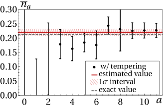
Figure 1: With tempering ($\beta\mu=5$) [4]. (Left) the sign averages at various replicas. The horizontal dashed line represents $3/\sqrt{2N_{\rm conf}}=0.017$. (Right) the data $\bar{n}_{a}$. The solid red line with a shaded band represents the estimate of $\langle n\rangle_{S}$ with $1\sigma$ interval. The gray dashed line represents the exact value.

We see that $\bar{n}_{a}$ take almost the same values for large $a$’s where the sign averages are well above the value $1/\sqrt{2N_{\rm conf}}$. The $\chi^{2}$ fit for $\{a\}=\{5,\ldots,11\}$ gives the estimate $\langle n\rangle_{S}\approx 0.221\pm 0.012$ (exact value: 0.212) with $\chi^{2}/{\rm DOF}=0.45$. Repeating this analysis for various $\beta\mu$, we obtain Fig. 2 [4].

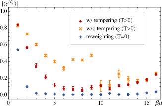
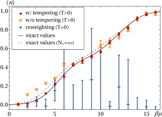
Figure 2: (Left) the sign averages at $T$, $|\langle e^{i\theta_{T}(x)}\rangle_{S^{\rm eff}_{T}}|$ [4]. (Right) the expectation values of the number density operator, $\langle n\rangle_{S}$ $(N_{\tau}=5)$ [4]. The results obtained with tempering correctly reproduce the exact values. The exact values for $N_{\tau}=\infty$ are also displayed for comparison.

We see that the exact values are correctly reproduced when the tempering is implemented, while there are significant deviations when not implemented. As in the $(0+1)$-dimensional massive Thirring model [3], the deviation reflects the fact that the relevant thimbles are not sampled sufficiently. This can be explicitly observed by looking at the distribution of flowed configurations (see Fig. 3).

Figure 3: The distribution of $\hat{z}\equiv(1/N)\sum_{i}z_{T}^{i}$ at $T=0.5$ for $\beta\mu=5$ [4]. (Left) with tempering. (Right) without tempering.

Two comments are in order [4]. (1) A larger value of the sign average does not necessarily mean a better resolution of the sign problem (see the left panel of Fig. 2).

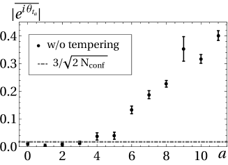
Figure 4: Without tempering ($\beta\mu=5$) [4]. (Left) the sign averages. (Right) the estimates $\bar{n}_{a}$.

In fact, when only a very few thimbles are sampled, the sign averages can become larger than the correctly sampled values due to the absence of phase mixtures among different thimbles. (2) From the right panel of Fig. 4, we see that it should be a difficult task to find such an intermediate flow time (without tempering) that avoids both the sign problem (severe at smaller flow times) and the ergodicity problem (severe at larger flow times. See [4] for more detailed discussions.

5 Conclusion and outlook

In this article, we reviewed the basics of the TLTM [3] and explained a new algorithm [4] which allows a precise estimation within the TLTM. We demonstrated its effectiveness by applying the TLTM to the two-dimensional Hubbard model away from half filling. Since the lattice we considered here is still small, it must be enlarged much more both in the spatial and imaginary time directions to claim the validity of our method for the sign problem in the Hubbard model, revealing its phase structure. In doing this, it should be important to check whether the computational scaling is actually $O(N^{3-4})$ as expected. More generally, we should keep developing the algorithm further so that the TLTM can be more easily applied to the three major problems listed in Introduction.

- [1] G. Aarts, Introductory lectures on lattice QCD at nonzero baryon number, J. Phys. Conf. Ser. 706 (2016) 022004 [1512.05145].
- [2] L. Pollet, Recent developments in Quantum Monte-Carlo simulations with applications for cold gases, Rep. Prog. Phys. 75 (2012) 094501 [1206.0781].
- [3] M. Fukuma and N. Umeda, Parallel tempering algorithm for integration over Lefschetz thimbles, PTEP 2017 (2017) 073B01 [1703.00861].
- [4] M. Fukuma, N. Matsumoto and N. Umeda, Applying the tempered Lefschetz thimble method to the Hubbard model away from half filling, Phys. Rev. D100 (2019) 114510 [1906.04243].
- [5] M. Cristoforetti, F. Di Renzo and L. Scorzato, New approach to the sign problem in quantum field theories: High density QCD on a Lefschetz thimble, Phys. Rev. D86 (2012) 074506 [1205.3996].
- [6] M. Cristoforetti, F. Di Renzo, A. Mukherjee and L. Scorzato, Monte Carlo simulations on the Lefschetz thimble: Taming the sign problem, Phys. Rev. D88 (2013) 051501(R) [1303.7204].
- [7] H. Fujii, D. Honda, M. Kato, Y. Kikukawa, S. Komatsu and T. Sano, Hybrid Monte Carlo on Lefschetz thimbles - A study of the residual sign problem, JHEP 1310 (2013) 147 [1309.4371].
- [8] A. Alexandru, G. Başar and P. Bedaque, Monte Carlo algorithm for simulating fermions on Lefschetz thimbles, Phys. Rev. D93 (2016) 014504 [1510.03258].
- [9] A. Alexandru, G. Başar, P. F. Bedaque, G. W. Ridgway and N. C. Warrington, Sign problem and Monte Carlo calculations beyond Lefschetz thimbles, JHEP 1605 (2016) 053 [1512.08764].
- [10] A. Alexandru, G. Başar, P. F. Bedaque and N. C. Warrington, Tempered transitions between thimbles, Phys. Rev. D96 (2017) 034513 [1703.02414].
- [11] A. Mukherjee and M. Cristoforetti, Lefschetz thimble Monte Carlo for many-body theories: A Hubbard model study, Phys. Rev. B90 (2014) 035134 [1403.5680].
- [12] Y. Tanizaki, Y. Hidaka and T. Hayata, Lefschetz-thimble analysis of the sign problem in one-site fermion model, New J. Phys. 18 (2016) 033002 [1509.07146].
- [13] M. Ulybyshev, C. Winterowd and S. Zafeiropoulos, Taming the sign problem of the finite density Hubbard model via Lefschetz thimbles, 1906.02726.
- [14] M. Ulybyshev, C. Winterowd and S. Zafeiropoulos, Lefschetz thimbles decomposition for the Hubbard model on the hexagonal lattice, 1906.07678.
- [15] R. H. Swendsen and J.-S. Wang, Replica Monte Carlo Simulation of Spin-Glasses, Phys. Rev. Lett. 57 (1986) 2607.
- [16] C. J. Geyer, Markov Chain Monte Carlo Maximum Likelihood, in Computing Science and Statistics: Proceedings of the 23rd Symposium on the Interface, American Statistical Association, New York, p. 156 (1991).
- [17] M. Fukuma, N. Matsumoto and N. Umeda, Implementation of the HMC algorithm on the tempered Lefschetz thimble method, 1912.13303.
- [18] M. Fukuma, N. Matsumoto and N. Umeda, Distance between configurations in Markov chain Monte Carlo simulations, JHEP 1712 (2017) 001 [1705.06097].
- [19] M. Fukuma, N. Matsumoto and N. Umeda, Emergence of AdS geometry in the simulated tempering algorithm, JHEP 1811 (2018) 060 [1806.10915].
- [20] M. Fukuma, N. Matsumoto and N. Umeda, Distance between configurations in MCMC simulations and the geometrical optimization of the tempering algorithms, PoS LATTICE2019 (2019) 168.
- [21] R. Blankenbecler, D. J. Scalapino and R. L. Sugar, Monte Carlo Calculations of Coupled Boson - Fermion Systems. 1., Phys. Rev. D24 (1981) 2278.