A Hybrid Approach to Temporal Pattern Matching

Abstract

The primary objective of graph pattern matching is to find all appearances of an input graph pattern query in a large data graph. Such appearances are called matches. In this paper, we are interested in finding matches of interaction patterns in temporal graphs. To this end, we propose a hybrid approach that achieves effective filtering of potential matches based both on structure and time. Our approach exploits a graph representation where edges are ordered by time. We present experiments with real datasets that illustrate the efficiency of our approach.

I Introduction

In this paper, we focus on graphs whose edges model interactions between entities. In such graphs, each edge is timestamped with the time when the corresponding interaction took place. For example, a phone call network can be represented as a sequence of timestamped edges, one for each phone call between two people. Other examples include biological, social and financial transaction networks. We are interested in finding patterns of interaction within such graphs. Specifically, we assume that we are given as input a graph pattern query $P$ whose edges are ordered and this order specifies the desired order of appearance of the corresponding interactions. We want to find all matches of $P$ in a temporal graph $G$, that is, the subgraphs of $G$ that match $P$ structurally, and whose edges respect the specified time order. We also ask that all interactions in the matching subgraph appear within a given time interval $\delta$. An example interaction pattern $P$ and temporal graph $G$ are shown in Fig. 1.

We propose an efficient algorithm which uses an edge-based representation of the graph where edges are ordered based on time. This representation allows fast pruning of the candidate matches that do not meet the temporal constraints. We then extent this representation to achieve combined structural and temporal pruning. Our experiments on four real datasets show the efficiency of our approach.

Related Work: There has been recent interest in processing and mining temporal graphs, including among others discovering communities [14], computing measures such as density [1, 12], PageRank [3, 9], and shortest path distances [4, 10, 13]. There have also been previous work on locating temporal motifs and subgraphs [2, 5, 6, 7, 8, 11, 15].

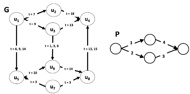
Figure 1: Temporal graph $G$ and graph pattern $P$. For clarity, multiple edges between nodes in $G$ are shown as a single edge with multiple timestamps.

The work in [11] introduces the problem of finding the most durable matches of an input graph pattern query, that is, the matches that exist for the longest period of time in an evolving graph. An algorithm for finding temporal subgraphs is provided in [5], with the restriction that edges in the motif must represent consecutive events for the node. Temporal cycles are studied in [6] and a heuristic approach for computing an estimation of the numbers of temporal motifs is studied in [2]. The authors of [8] consider a query graph with non time-stamped edges and define as temporal match a subgraph such that all its incoming edges occur before its outgoing edges.

Most closely related to ours is the work in [7], and [15]. The authors of [15] index basic graph structures in the static graph so as to find a candidate set of isomorphic subgraphs quickly at query time, and then verify for each candidate match whether the time conditions hold. The authors of [7] use as similar to ours time ordered representation of the temporal graph but they locate the temporal graphs by a static subgraph matching algorithm and then use a separate algorithm to find all temporal subgraph matches. In summary, these works enumerate matches of a pattern graph using a two phase approach: they first perform structural matching and then they filter the results that do not meet the time conditions. Our work proposes a combined structural-temporal matching approach.

II Problem definition

A temporal graph $G(V,E)$ is a directed graph where $V$ is a set of nodes, $E$ is a set of temporal edges $(u,v,t)$ where $u$ and $v$ are nodes in $V$, and $t$ is a timestamp in $\mathbb{R}$. There may be multiple temporal edges between a pair of nodes capturing interactions appearing at different time instants. An example is shown in Fig. 1.

We use $\Pi(u,v)$ to denote the set of edges from $u$ to $v$, $\pi(u,v)$ the number of such edges, and $time(e)$ the timestamp of temporal edge $e$. For example in Fig. 1, the nodes $u_{1},u_{5}$ are connected through three edges, e.g, $\Pi(u_{1},u_{5})=\{e_{1},e_{2},e_{3}\}$ with $time(e_{i})=6,time(e_{2})=9$, and $time(e_{3})=14$.

The same timestamp may appear more than once modeling simultaneous interactions. Thus, timestamps impose a partial order $\prec_{\textsc{t}}$ on temporal edges. For a pair of temporal edges, $e_{i}$ and $e_{j}$ in $E$, $e_{i}$ $\prec_{\textsc{t}}$ $e_{j}$, if $time(e_{i})$ $<$ $time(e_{j})$ and $e_{i}$ $=_{\textsc{t}}$ $e_{j}$, if $time(e_{i})$ $=$ $time(e_{j})$.

We define the start time, $start\_time(G)$, and end time, $end\_time(G)$, of a temporal graph $G$ as the smallest and largest timestamp appearing in any of the temporal edges in $E$. We also define the duration, $dur(G)$ of a temporal graph as $end\_time(G)$ - $start\_time(G)+1$.

We are interested in finding patterns of interactions in a temporal graph that appear within a time period of $\delta$ time units. A $\delta$-interaction pattern $P$ is a temporal graph with $dur(P)$ $\leq$ $\delta$.

Definition 1

[Interaction Pattern Matching] Given a temporal graph $G(V,E)$, a time window $\delta$ and a $\delta$-interaction pattern $P$ = $G(V_{P},E_{P})$, a subgraph $M$ = $G(V_{M},E_{M})$ of $G$ is a match of $P$, such that the following conditions hold:

1. (subgraph isomorphism) There exists a bijection $f$: $V_{P}\rightarrow V_{M}$ such that, there is a one-to-one mapping between the edges in $E_{P}$ and $E_{M}$, such that. for each edge ($u$, $v$, $t$) in $E_{P}$, there is exactly one edge ($f(u)$, $f(v)$, $t^{\prime}$) in $E_{M}$,

2. (temporal order preservation) For each pair of edges $e_{1}$ and $e_{2}$ in $E_{P}$ mapped to edges $e^{\prime}_{1}$ and $e^{\prime}_{2}$ in $E_{M}$, it holds $e_{1}$ $\prec_{\textsc{t}}$ $e_{2}$ $\Rightarrow$ $e^{\prime}_{1}$ $\prec_{\textsc{t}}$ $e^{\prime}_{2}$ and $e_{1}$ $=_{\textsc{t}}$ $e_{2}$ $\Rightarrow$ $e^{\prime}_{1}$ $=_{\textsc{t}}$ $e^{\prime}_{2}$.

3. (within $\delta$) $dur(M)$ $\leq$ $\delta$.

For example, in Fig. 1, the subgraph $G^{\prime}$ induced by $\{u_{1},u_{2},u_{3},u_{4}\}$ is a match of $P$ with $dur(G^{\prime})=12$.

III Algorithms

We call static graph the directed graph $G_{S}(V,E_{S})$ induced from temporal graph $G(V,E)$, if we ignore timestamps and multiple edges, i.e., $(u,v)$ is an edge in $E_{S}$, if and only if, there is a temporal edge $(u,v,t)$ in $E$.

A straightforward approach is to apply a graph pattern matching algorithm on the static graph $G_{S}$ and then for each match find all time-ordered matches. However, it is easy to see that for a match $M_{S}$ in $G_{S}$, the number of candidate time-ordered matches can be up to $\prod_{i=1}^{|E_{M_{S}}|}\pi(e^{M_{S}}_{i})$, for each $e_{i}\in M_{S}$. In the following, we introduce an alternative approach.

III-A Interaction Pattern Matching

Our pattern matching algorithm identifies the interaction pattern matches by traversing a representation of the graph where edges are ordered based on $\prec_{\textsc{t}}$. Let $L_{G}$ be this representation, that is, the list of graph edges of $G$ ordered by $\prec_{\textsc{t}}$. We also order by $\prec_{\textsc{t}}$ the edges in the pattern, let $L_{P}$ = $e^{P}_{1},\dots e^{P}_{|E_{P}|}$ be the resulting list. We match pattern edges following the order specified in the input pattern. The algorithm matches the edges in the pattern edge-by-edge in a depth-first manner until all edges are mapped and a full matching subgraph is found. The basic steps are outlined in Algorithm 1. We use a stack $S$ to maintain the graph edges that have been mapped to pattern edges so far. Index $i$ denotes the pattern edge to be mapped next. MatchingEdge performs two types of pruning:

1. temporal pruning: matched edges must (a) follow the time-order and (b) be within $\delta$.

2. structural pruning: the matched graph must be isomorphic to the pattern subgraph.

Next, we describe a simple variation of MatchingEdge termed SimpleME and then a more efficient one termed IndexME.

Algorithm 1 InteractionSearch($G$, $P$, $\delta$)

1:Temporal graph $L_{G}$, pattern graph $L_{P}$, time window $\delta$

2:Interaction matches $m$  

3:$S\leftarrow\emptyset$ $\triangleright$ stack with candidate matches

4:$M\leftarrow\emptyset$ $\triangleright$ interaction matches

5:$sT\leftarrow\delta$ $\triangleright$ remaining time

6:$MoreMatches$ $\leftarrow$ $True$; $i$ $\leftarrow$ $1$

7:while $(MoreMatches)$ do

8:    $e^{G}_{i}\leftarrow$ MatchingEdge$(e^{P}_{i},sT)$

9:    if $e^{G}_{i}\neq null$ then

10:         $Push(e^{G}_{i},S)$

11:         if $i=|E_{P}|$ then $\triangleright$ a compete match is found

12:             $M$ $\leftarrow$ $M$ $\cup$ $Content(S)$

13:             $i$ $\leftarrow$ 1

14:         else$~{}~{}i\leftarrow i+1$; $sT\leftarrow sT-time(e^{G}_{i})$          

15:    else$\triangleright$ no match found

16:         if $i=1$ then $MoreMatches$ $\leftarrow$ $False$

17:         else$~{}~{}Pop(S)$; $i\leftarrow i-1$              

Simple Temporal-Structural filtering. SimpleME shown in Algorithm 2 scans the graph edges in $L_{G}$ linearly. The key idea is that when we have matched the $i$-th pattern edge with a graph edge at position $j$, to match the next $i+1$-th pattern edge, we need to look only at positions in $L_{G}$ larger than $j$. As we build the match, we maintain the mapping $F$ of pattern edges to graph edges. We use $F(u)$ to denote the graph node that pattern node $u$ was mapped to. If $u$ is not yet mapped, $F(u)$ is $null$.

Algorithm 2 SimpleME($(u^{P},v^{P})$, $rT$)

1:Pattern edge $(u^{P},v^{P})$ to be mapped, remaining time $rT$, mapping $F$ of pattern nodes to graph nodes, position in the graph of the previously matched edge $i^{G}$

2:Graph edge $(u^{G},v^{G})$ matching pattern edge $(u^{P},v^{P})$  

3:for ($i=i^{G}+1$ to $max$) do

4:    $(u^{G},v^{G})=L_{G}[i]$

5:    if ($time(u^{G},v^{G})$ $\leq$ $rT$) then

6:         if $(F(u^{P})=F(u^{P})=null$) or $(F(u^{P})=null$ and $F(v^{P})=v^{G})$ or $(F(v^{P})=null$ and $F(u^{P})=u^{G}$) or $(F(u^{P})=u^{G}$ and $F(v^{P})=v^{G}$)  then

7:             $i^{G}=i$ $\triangleright$ matching edge found

8:             Update map $F$

9:             return ($(u^{G},v^{G})$)          

10:    else

11:         $i$ $\leftarrow$ $i$ + 1     

12:return (null) $\triangleright$ no matching edge found

Let $i_{G}$ denote the last position in $L_{G}$ where a graph edge has been mapped to a pattern edge. In SimpleME, we just go through the edges of the graph starting just after the position of the previously matched edge (position $i^{G}$ + 1). For each edge, we check whether the edge satisfies the temporal and graph isomorphism conditions. The maximum number of edges to be checked is equal to the number of edges $e_{i}$ for which $time(e_{i})\leq rT+time(e_{i^{G}})$. For example, if $rT=5$ and the time of the last mapped edge is 4 then only the edges $e_{i}$ with $time(e_{i})\leq 9$ should be checked.

Indexed temporal-structural filtering. IndexME uses information about the ingoing and outgoing edges of each node to avoid the linear scanning of the graph. Two structures are used: (a) an additional mapping structure $F_{edge}$, and (b) an extension of the graph structure $L_{G}$ with neighborhood information.

Specifically, in addition to the mapping table $F$, we maintain a mapping table $F_{edge}$. Assume that pattern node $u^{P}$ during the course of the algorithm is mapped to graph node $u^{G}$. We maintain the matching graph edge $u^{G}$ in $F(u^{P})$, and also in $F_{edge}(u^{P})$ the most recently matched graph edge for which $u^{G}$ was either a source node or a target node. Note that this edge is also the most recent edge. All graph edges that will match the remaining pattern edges must appear later in time than this edge.

We also extend $L_{G}$. For each edge $e^{G}$ = $(u^{G},v^{G})$ in $L_{G}$, we maintain in $N_{s}(u^{G},e)$ the next in time edge with source node $u^{G}$, in $N_{t}(u^{G},e)$ the next in time edge with target node $u^{G}$ and similarly $N_{s}(v^{G},e)$ and $N_{t}(v^{G},e)$ for node $v^{G}$. We can retrieve all in and out neighbors of a node ordered by time by simply following these lists. For example, to find the out-neighbors of node $u$, we start by the first edge, say $e$, where $u$ appears, retrieve $N_{s}(u,e)$, then $N_{s}(u,N_{s}(u,e))$ and so on. We will use the notation $next_{in}(u)$ ($next_{out}(u))$ to denote getting the next in-neighbor (resp. out-neighbor) of $u$. Note, that each edge is represented by its position in the $L_{G}$ graph.

Algorithm 3 IndexME($(u^{P},v^{P})$, $rT$)

1:Pattern edge $(u^{P},v^{P})$ to be mapped, remaining time $rT$, mapping $F$ of pattern nodes to graph nodes, position in the graph of the previously matched edge $i^{G}$, list $L_{in}$ and $L_{out}$

2:Graph edge $(u^{G},v^{G})$ matching pattern edge $(u^{P},v^{P})$  

3:if $F(u^{P})=null$ and $F(v^{P})=null$ then

4:    for ($i=i^{G}+1$ to $max$) do

5:         $(u^{G},v^{G})=L_{G}[i^{G}]$

6:         if ($time(u^{G},v^{G})$ $\leq$ $rT$) then

7:             $i^{G}=i$ $\triangleright$ matching edge found

8:             Update $F(u^{P})$, $F_{edge}(u^{P})$, $F(v^{P})$, $F_{edge}(v^{P})$

9:             return ($(u^{G},v^{G})$)

10:         else$~{}~{}i$ $\leftarrow$ $i$ + 1              

11:    return (null) $\triangleright$ no matching edge found

12:else if $F(u^{P})\neq null$ and $F(v^{P})\neq null$ then

13:    $j$ $\leftarrow$ $max\{F_{edge}(u^{P}),F_{edge}(v^{P})\}$

14:    for ($i=j$ to $max$) do

15:         if $j$ = $F_{edge}(u^{P})$ then

16:             search the out-neighbors of $N_{s}(L_{G}[j]$ to find $F(v^{P})$

17:         else   search the in-neighbors of $N_{t}(L_{G}[j]$ to find $F(u^{P})$          

18:         Let $m$ be the edge found

19:         if ($time(m)$ $\leq$ $rT$) then

20:             $i^{G}=m$ $\triangleright$ matching edge found

21:             Update $F_{edge}(u^{P})$, $F_{edge}(v^{P})$

22:             return ($(m)$)

23:         else$~{}~{}i$ $\leftarrow$ $i$ + 1              

24:    return (null) $\triangleright$ no matching edge found

25:else if $F(u^{P})\neq null$ then

26:    search as above using next out $N_{s}(L_{G}[j])$

27:else$~{}~{}i$ search as above using next in $N_{t}(L_{G}[j])$

Let us now describe the IndexME algorithm (shown in Algorithm 3) in detail. The algorithm first checks whether any of the pattern edge endpoints has already been mapped. If none of them has already been matched, then in Lines 2-9, it searches for any match satisfying the time constraints in Line 4. Otherwise, if both endpoints have been matched in Lines 10-22, we get one of the endpoints, let this be node $u$ and depending on whether it is a source or a target node, either the $next_{out}(u)$ or $next_{in}(u)$ is used to find the edges containing the other endpoint in Lines 13-15. Next, if the mapped edge is active within the remaining time window the algorithm updates the matched edge index structure and returns the edge in Lines 17-20. In case just one of the two endpoints is matched, say $u$, we follow the same steps for missing endpoint $v$ by looking into the in-neighbor (resp. out-neighbor) lists of $u$ in Lines 23-25.

IV Experimental Evaluation

We use the following real datasets [7]: (1) Email-EU contains emails between members of a European research institution; an edge indicates an email send from a person $u$ to a person $v$ at time $t$. (2) FBWall records the wall posts between users on Facebook located in the New Orleans region; each edge indicates the post of a user $u$ to a user $v$ at a time $t$. (3) Bitcoin refers to the decentralized digital currency and payment system. It consists of all payments made up to October 19, 2014; an edge records the transfer of a bitcoin from address $u$ to address $v$ at a time $t$. (4) Superuser records the interactions on the stack exchange web site Super User; edges indicate the users’ answers/comments/replies to comments. The characteristics of the datasets are summarized in Table I.

TABLE I: Dataset characteristics

Dataset	# Nodes	# Static Edges	Edges	# Time (days)
Email-EU	986	24,929	332,334	803
FBWall	46,952	274,086	876,993	1,506
Bitcoin	1,704	4,845	5,121,024	1,089
Superuser	194,085	924,886	1,443,339	2,645

TABLE II: Execution time (sec) of $IPM$ and $Competitor$ for varying time window $\delta$ and path lengths.

	Email-EU		FBWall		Bitcoin		Superuser
$\delta$ (hours)	IPM	Comp	IPM	Comp	IPM	Comp	IPM	Comp
$\delta=1$	1.45	21	3.72	42	1.48	15.7	4.07	45
$\delta=3$	1.56	49	3.85	65	4.24	135	4.92	66
$\delta=6$	1.86	115	3.92	105	15.7	675	4.94	101
$\delta=9$	2.85	171	4.17	132	48.8	$>$ 0.5h	5.3	127
$\delta=12$	3.41	190	4.65	152	113	$>$ 0.5h	5.5	160
Path length	IPM	Comp	IPM	Comp	IPM	Comp	IPM	Comp
$l=2$	0.05	0.3	3.4	10	1	6.5	3.35	15
$l=4$	0.9	1.05	3.5	28	1.1	10	3.8	18
$l=6$	1.45	21	3.72	42	1.48	15.7	4.07	45
$l=8$	1.9	103	4	80	1.63	28	4.93	110
$l=10$	2.2	115	4.28	85	1.72	36	5.53	121

Results: We first compare our algorithm, termed $\sc{IPM}$, with the competitive approach followed in [7, 8] which first generates the candidate subgraphs that match the topology of the pattern and then filters the results that do not follow the specified temporal order. The generation of candidate subgraphs is done edge by edge and only the matches active within the $\delta$ time window are retained. As our default pattern queries, we use two type of queries: (a) path queries, and (b) random graph pattern queries. Path pattern queries represented as a sequence of edges with consequent timestamps. Random graph pattern queries are generated as follows. For a random query of size $n$, we select a node randomly from the graph and starting from this node, we perform a DFS traversal until the required number n of nodes is visited. We use as our pattern, the graph created by the union of visited nodes and traveled edges. We set the ordering of edges using the topological ordering of the graph. We report the average performance of 100 random queries for each size n.

Table II reports the results a) for various $\delta$ (for $\delta=1$ up to $12$ hours) and path length = 6, and b) for various path lengths (from 2 up to 10) and fixed $\delta=1$ hour. As shown, the $Competitor$’s response time increases with $\delta$, while $\sc{IPM}$ is considerably faster in all datasets. This is because the $Competitor$ tends to generate many redundant matches which do not follow the required temporal order. This is more prominent when we increase the query duration $\delta$. Also, there are cases where a found match $m$ contains edges with multiple timestamps and thus the algorithm must generate a large number of temporal matches. This is the case especially with the Bitcoin and the Email-EU datasets, where there are multiple timestamped edges per static edge. Regarding the path length, the $Competitor$’s response time is increasing with the path length while, again, $\sc{IPM}$ is considerably faster and not affected much by the query size. $\sc{IPM}$ takes advantage of the indexes and verifies for each edge with a few lookups whether there is any other valid edge within the remaining time window. Similar results hold for random queries.

(a) Bitcoin

(b) Superuser

Figure 2: Query time for random queries for various query sizes.

Fig. 2 reports the performance of our algorithm for random queries of different graph sizes $Qn$ (from $n=2$ up to $n=10$ nodes) and different time windows. All small queries are processed very fast because the algorithm requires only a few lookups to identify adjacent nodes within the given time window. Moreover, even for largest queries and longest timer windows where larger lookups are required, our algorithm only takes $\sim$2 and $\sim$10 minutes to process the query in Bitcoin and Superuser respectively. The performance difference in Superuser dataset is expected since it consists of a much larger number of edges and time instants than Bitcoin.

V Conclusions

In this paper, we studied the problem of locating matches of patterns of interactions in temporal graphs that appear within a specified time period. We presented an efficient algorithm based on a representation of graph where edges are ordered based on their interaction time. Our experimental evaluation with real datasets demonstrated the efficiency of our algorithm in finding time-ordered matches. In the future, we plan to study the streaming version of the problem where given a stream of graph updates we locate the interaction patterns occurring within a sliding time window.

References

- [1] Edoardo Galimberti, Alain Barrat, Francesco Bonchi, Ciro Cattuto, and Francesco Gullo. Mining (maximal) span-cores from temporal networks. In CIKM, pages 107–116, 2018.
- [2] Saket Gurukar, Sayan Ranu, and Balaraman Ravindran. COMMIT: A scalable approach to mining communication motifs from dynamic networks. In ACM SIGMOD, pages 475–489, 2015.
- [3] Weishu Hu, Haitao Zou, and Zhiguo Gong. Temporal pagerank on social networks. In WISE, pages 262–276, 2015.
- [4] Wenyu Huo and Vassilis J. Tsotras. Efficient temporal shortest path queries on evolving social graphs. In SSDBM, pages 38:1–38:4, 2014.
- [5] Lauri Kovanen, Márton Karsai, Kimmo Kaski, János Kertész, and Jari Saramäki. Temporal motifs in time-dependent networks. Journal of Statistical Mechanics: Theory and Experiment, 2011(11):P11005, 2011.
- [6] Rohit Kumar and Toon Calders. 2scent: An efficient algorithm to enumerate all simple temporal cycles. PVLDB, 11(11):1441–1453, 2018.
- [7] Ashwin Paranjape, Austin R. Benson, and Jure Leskovec. Motifs in temporal networks. In WSDM, pages 601–610, 2017.
- [8] Ursula Redmond and Pádraig Cunningham. Temporal subgraph isomorphism. In ASONAM, pages 1451–1452, 2013.
- [9] Polina Rozenshtein and Aristides Gionis. Temporal pagerank. In ECML PKDD, pages 674–689, 2016.
- [10] Konstantinos Semertzidis and Evaggelia Pitoura. Historical traversals in native graph databases. In ADBIS, pages 167–181, 2017.
- [11] Konstantinos Semertzidis and Evaggelia Pitoura. Top-k durable graph pattern queries on temporal graphs. IEEE Trans. Knowl. Data Eng., 31(1):181–194, 2019.
- [12] Konstantinos Semertzidis, Evaggelia Pitoura, Evimaria Terzi, and Panayiotis Tsaparas. Finding lasting dense subgraphs. Data Min. Knowl. Discov., 33(5):1417–1445, 2019.
- [13] Huanhuan Wu, James Cheng, Silu Huang, Yiping Ke, Yi Lu, and Yanyan Xu. Path problems in temporal graphs. PVLDB, 7(9):721–732, 2014.
- [14] Ding Zhou, Isaac G. Councill, Hongyuan Zha, and C. Lee Giles. Discovering temporal communities from social network documents. In ICDM, pages 745–750, 2007.
- [15] Andreas Züfle, Matthias Renz, Tobias Emrich, and Maximilian Franzke. Pattern search in temporal social networks. In EDBT, pages 289–300, 2018.