Theoretical investigation of the bow shock location for the solar wind interacting with the unmagnetized planet

Abstract

Martian bow shocks, the solar wind interacting with an unmagnetized planet, are studied. We theoretically investigated how solar parameters, such as the solar wind dynamic pressure and the solar extreme ultraviolet (EUV) flux, influence the bow shock location, which is still currently not well understood. We present the formula for the location of the bow shock nose of the unmagnetized planet. The bow shock location, the sum of the ionopause location and bow shock standoff distance, is calculated in the gasdynamics approach. The ionopause location is determined using thermal pressure continuity, i.e., the solar wind thermal pressure equal to the ionospheric pressure, according to tangential discontinuity. The analytical formula of the ionopause nose location and the ionopause profile around the nose are obtained. The standoff distance is calculated using the empirical model. Our derived formula shows that the shock nose location is a function of the scale height of ionosphere, the dynamic pressure of the solar wind and the peak ionospheric pressure. The theoretical model implies that the shock nose location is more sensitive to the solar EUV flux than solar wind dynamics pressure. Further, we theoretically show that the bow shock location is proportional to the solar wind dynamic pressure to the power of negative C, where C is about the ratio of the ionospheric scale height to the distance between bow shock nose and the planet center. This theory matches the gasdynamics simulation and is consistent with the spacecraft measurement result by Mars Express [Hall, et al. (2016) J. Geophys. Res. Space Physics, 121, 11,474-11,494].

Keywords: bow shock of the unmagnetized planet, standoff distance, ionosphere, ionopause, gasdynamics theory

¹Department of Physics, UC San Diego, USA

²Institute of Space and Plasma Sciences, National Cheng Kung University, Taiwan

1 Introduction

In the nowadays space physics research, more research focuses on the solar wind interacting with the magnetized planet than the unmagnetized planet or weakly-magnetized planet. However, the study of Martian bow shock is recently a hot topic due to the growing interests in the exploration of Mars, a weakly-magnetized planet. Furthermore, more and more data from the spacecraft measurement are available. A theoretical model of the bow shock nose position has been derived in this work.

There are three types of interaction between the solar wind and an obstacle in space: (1) solar wind interacting with the magnetized obstacle like Earth. (2) solar wind interacting with the unmagnetized obstacle with an atmosphere like Mars and Venus. (3) solar wind interacting with the unmagnetized obstacle without atmosphere like moon. Figure 1 is a schematic of these three types of interaction.

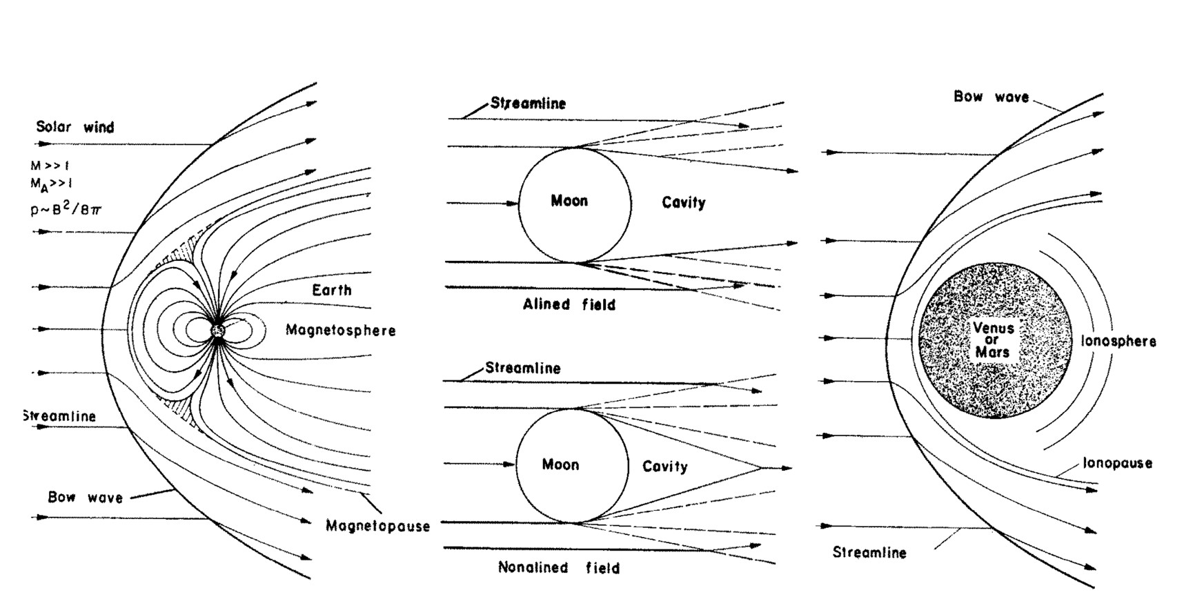
Figure 1: Schematic of solar wind past the (a) Earth (b) Moon (c) Mars and Venus. Courtesy of Ref. [1].

The detached bow shock is formed because of the supersonic solar wind and the deflection of the incident solar wind flow by the magnetosphere or ionosphere. Since the moon has neither ionosphere nor magnetosphere, no bow shock is formed in the solar wind interacting with the moon.

Formation of the bow shock in plasma interaction with Mars, unmagnetized planets with an atmosphere (Fig. 2), is as follows. First, the ionization by solar EUV radiation in the atmosphere forms an ionospheric obstacle, acting as a conductor. The boundary of the ionosphere is called ionopause. Then the solar-wind plasma with its frozen-in field flows at a supersonic velocity toward the conducting obstacle, resulting in the appearance of the bow shock.

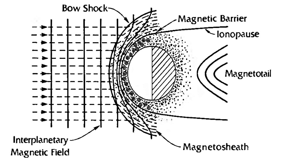
Figure 2: Schematic of the solar wind interaction with an unmagnetized planet with an atmosphere. Courtesy of Ref.[2].

Martian bow shock has been detailedly studied by spacecraft measurement and numerical simulation. Martian bow shock is formed by the interaction between the solar wind and the Martian ionosphere. Recently, the first measurement study[3] of the ionopause from the mission Mars Atmosphere and Volatile EvolutioN (MAVEN, 2014-present) was released in 2015. This mission will provide us a deeper understanding of the Martian bow shock. The shape of the bow shock is often modeled using the least-squares fitting of an axisymmetric or non-axisymmetric conic section[4, 5] with the data from spacecraft measurement. On the other hand, the theoretical model of the planetary bow shock location and shape can be seen in the review paper by Spreiter[1, 6, 7], Slavin[8, 9] and Verigin[10]. An efficient computational model for determining the global properties of the solar wind past a planet based on axisymmetric magnetohydrodynamics was proposed by Spreiter[11]. The specific study of the magnetohydrodynamics simulation for the solar wind interaction with Mars can be seen in Ref.[12] and Ref.[13].

However, how the factors influence the location of the Martian bow shock is not well understood. The main factors impacting the bow shock position are the solar wind dynamic pressure $P_{dyn}=\rho_{\infty}v_{\infty}^{2}$ and solar EUV flux $l_{euv}$. According to the fitting results (Fig. 3) from the data of Mars Express Analyser of Space Plasma and EneRgetic Atoms (ASPERA-3)[14], it is shown that the bow shock location ($r_{s}$) reduces in altitude with increasing solar wind dynamic pressure in the relation $r_{s}\propto P_{dyn}^{-0.02}$ and increases in altitude with increasing solar EUV flux in the relation $r_{s}\propto 0.11\,l_{EUV}$. It means that the bow shock position is more sensitive to the solar EUV flux than the solar wind dynamic pressure.

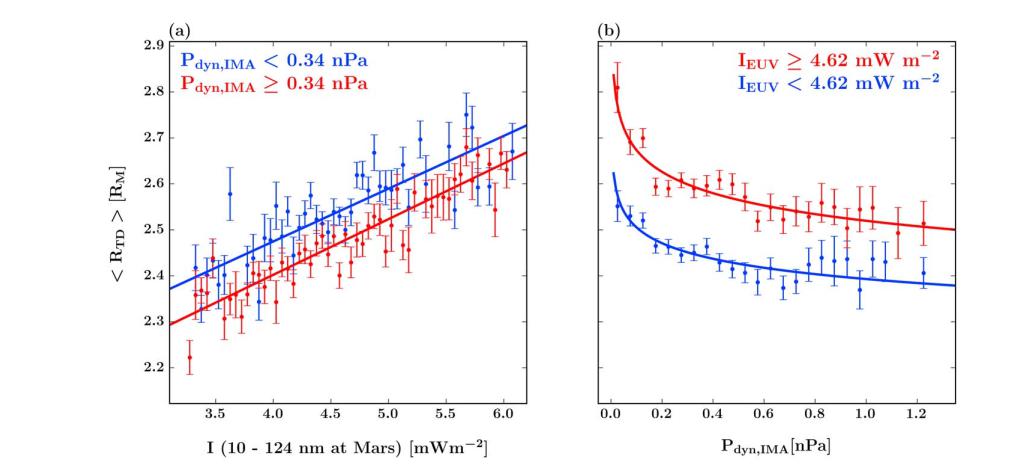
Figure 3: The response of the location of the Martian bow shock with the solar parameters. (a) Bow shock location against solar EUV radiance. (b) Bow shock location against solar wind dynamic pressure. Courtesy of [14].

Other parameters controlling the Martian bow shock location are the intense localized Martian crustal magnetic fields[15], the magnetosonic Mach number[16], the interplanetary magnetic fields and the convective electric field[17]. In this thesis, we will mainly focus on the dependence of the solar wind dynamics pressure and the ionospheric pressure, which is dependent on the solar EUV radiation.

It is not well understood how the location of the Martian bow shock is influenced by the solar parameters such as solar wind dynamic pressure and EUV flux. In this thesis work, we study the location of the bow shock generated from the interaction between the solar wind and unmagnetized planet in the theoretical aspect. The formula for the shock nose location as a function of the solar wind dynamic pressure and EUV flux will be presented and compared with the spacecraft measurement. Past studies by others are all related to observation, but this study provides a theory to explain the spacecraft measurement results. On the other hand, we are not going to study fine structure in the transition region of a shock and the shock microphysics, even though it is more theoretically fascinating. The dissipation mechanism for the shock will not influence the location of the bow shock, so we use the ideal hydrodynamics formulation throughout this work. Note that the thickness of the discontinuity surface is zero under the ideal hydrodynamics description.

The analytical theory is essential because the relationship between each physical quantities can be directly known in the formula. However, in simulation, to know the results from different conditions requires different runs, which is very numerically intensive especially for multi-scale and multi-physics simulation. This work will be beneficial for both space physics and laboratory astrophysics research. In laboratory astrophysics research.

In this paper, we will focus on theoretically determining the location of the nose of the bow shock for the solar wind past the unmagnetized planet. The formula for shock nose location is developed and compared to the results from the hydrodynamics simulation and spacecraft measurement. In section 2, we will give a detailed derivation of the formula for the shock nose position. The comparison of our formula and the spacecraft measurement results will be shown in section 3. In section 4, the conclusion of the thesis will be given.

2 Determination of the location of the bow shock nose

We theoretically investigate the bow shock location as a function of the solar wind and the ionospheric conditions, such as solar wind dynamic pressure $\rho_{\infty}v_{\infty}^{2}$, ionospheric scale length $H$, ionospheric peak pressure $P_{M,i}$ and the location of the ionospheric peak pressure $r_{M,i}$. The equation of bow shock location is derived and will be used to design the future experiments. We only focus on the nose location of the bow shock but not the whole shape profile of the bow shock. The shape of the bow shock and the ionopause is assumed to be symmetric around the x-axis.

The schematic of the bow shock and the obstacle boundary (ionopause) is shown in the Fig. 4. We use the following symbols to represent the geophysical quantities in the report: $r_{o}$ is nose positions of the obstacle, $r_{s}$ is nose positions of the bow shock, $r_{M,i}$ is the location inside ionosphere where maximal thermal pressure occurs, $\Delta$ is the bow shock standoff distance, i.e., the distance between ionopause nose position and bow shock nose position.

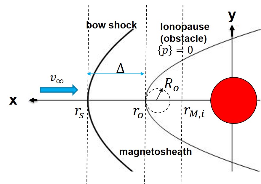
Figure 4: Definition of each variable used in the report

The goal is to determine the shock nose location $r_{s}$:

$$r_{s}=r_{o}+\Delta.$$ (1)

Ionopause nose location $r_{o}$ is calculated using the continuity of the thermal pressure by tangential discontinuity[1, 6, 10]; bow shock standoff distance is calculated by the empirical formula[4, 10].

We first introduce the hydrodynamics boundary conditions in subsection 2.1. The derivation of the ionopause nose location and the radius of curvature at ionopause nose are in subsection 2.3. The standoff distance formula is introduced in subsection 2.4. Finally, the formula of the bow shock nose location is shown in subsection 2.5. The comparison of the theory and the observation results will be given in next section (section 3).

2.1 Hydrodynamics boundary condition

Hydrodynamics formulation is used throughout this thesis. Ideal magnetohydrodynamics equations are

$$\frac{\partial\rho}{\partial t}+\nabla\cdot\rho\,\vec{v} =0,$$

$$\rho(\frac{\partial\vec{v}}{\partial t}+\vec{v}\cdot\nabla v) =-\nabla P+\frac{1}{\mu_{0}}(\nabla\times\vec{B})\times\vec{B},$$

$$\frac{\partial\vec{B}}{\partial t} =\nabla\times\vec{v}\times\vec{B},$$

$$\frac{\partial P}{\partial t}+\vec{v}\cdot\nabla P =-\gamma\,P\>\nabla\cdot\vec{v},$$ (2)

where $p$ is the pressure, $\rho$ is the mass density, $\vec{v}$ is the velocity and $\vec{B}$ is the magnetic field. The first one is the continuity equation, the second is the momentum equation, the third is Faraday’s law and the last is the entropy conservation equation, or adiabatic equation. Here we assume the gas follows the polytropic condition and adiabatic process.

Magnetohydrodynamics equations can be reduced to hydrodynamics equations under the condition that the magnetic pressure term is much smaller than the thermal pressure term in the right-hand side of the momentum equation (second equation in Eq. 2)

$$|\frac{\frac{1}{\mu_{0}}(\nabla\times\vec{B})\times\vec{B}}{\nabla P}|\approx\frac{B^{2}/2\mu_{0}}{P}=1/\beta,$$ (3)

where plasma beta $\beta$ is defined as thermal pressure divided by magnetic pressure. For the condition of solar wind past the unmagnetized planet, $\beta$ is much larger than 1 in both space and laboratory, so we can neglect the force term containing the magnetic field in the momentum equation, reducing the magnetohydrodynamics formulation to pure hydrodynamics formulation

$$\frac{\partial\rho}{\partial t}+\nabla\cdot\rho\,\vec{v} =0,$$

$$\rho(\frac{\partial\vec{v}}{\partial t}+\vec{v}\cdot\nabla v) =-\nabla p,$$

$$\frac{\partial P}{\partial t}+\vec{v}\cdot\nabla P =-\gamma\,P\>\nabla\cdot\vec{v.}$$ (4)

Throughout the paper, we will use hydrodynamics formulation instead of magnetohydrodynamics due to the high beta condition. The first one is the mass conservation equation, the second is the momentum equation for ideal fluid, or Euler equation and the third is the adiabatic equation.

The boundary condition for steady-state ideal hydrodynamics[18] is

$$\left[\rho v_{n}\right] =0$$

$$\left[P+\rho v_{n}^{2}\right] =0$$

$$\left[\rho v_{n}\vec{v_{t}}\right] =0$$

$$\left[v_{n}(\frac{\rho v^{2}}{2}+\frac{\gamma\,P}{\gamma-1})\right] =0,$$ (5)

where the subscript $n$ and $t$ are the normal direction and tangential direction, respectively. The brackets mean the difference of the quantity between both sides of the boundary. The Eq. 5 indicates the continuity of the mass flux, momentum flux and energy flux. Note that the discontinuity surfaces of the ionopause and the bow shock are zero thickness under the description of the dissipationless ideal (magneto)hydrodynamics[18, 19].

In our study, we are interested in two types of boundary:

• Tangential discontinuity[1, 6, 18] at the ionopause

  $$\left[\rho\right]\neq 0$$

  $$\left[\vec{v_{t}}\right]\neq 0$$

  $$v_{n}= 0$$

  $$\left[P\right]= 0.$$ (6)

  The normal velocity is zero in the tangential discontinuity. We will utilize the continuity of the thermal pressure to determine the location and the radius of curvature at the ionopause nose. Furthermore, we can observe that there is a density jump across the ionopause according to tangential discontinuity.

• Shock waves[1, 6, 18] at the bow shock front

  $$\left[\rho v_{n}\right]= 0$$

  $$\left[\vec{v_{t}}\right]= 0$$

  $$\left[P+\rho v_{n}^{2}\right]= 0$$

  $$\left[\frac{v_{n}^{2}}{2}+\frac{\gamma\,P/\rho}{\gamma-1}\right]= 0.$$ (7)

  For our purpose of the study of the global phenomenon like bow shock position, the ideal fluid description is enough. We are not going to study microphysics such as the shock formation mechanism, so the dissipation process of the shock will not be discussed throughout the thesis. In general, the shock in the space is formed in a collisionless magnetized environment and the shock dissipation mechanism is the wave-particle interaction.

2.2 Overview of the theory

In this subsection, we have an overview of all the theories which are used for calculating the location of the bow shock nose in terms of the solar wind and the ionospheric conditions. Fig. 5 shows the variation of the thermal pressure along the stagnation streamline.

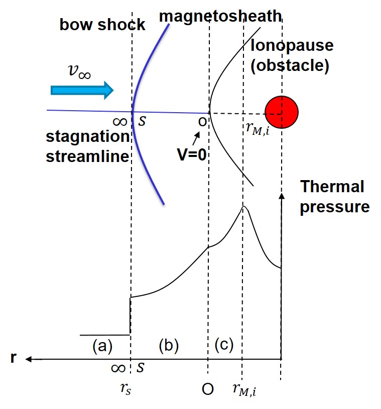
Figure 5: Thermal pressure along the stagnation streamline.

• (a) Solar wind

  • In the region of the solar wind, the thermal pressure can be expressed as a function of the dynamic pressure and the sonic Mach number, i.e., $P_{\infty}=\rho_{\infty}v_{\infty}^{2}/(M_{\infty}^{2}\,\gamma)$.

• (a) – (b) Bow shock

  • At the bow shock, momentum flux conservation in the normal shock relation is used

    $$P_{\infty}+\rho_{\infty}v_{\infty}^{2}=P_{s}+\rho_{s}v_{s}^{2}.$$ (8)

    Note that the entropy increases across the shock.

• (b) Magnetosheath

  • Within the magnetosheath, the plasma follows the process of the isentropic compression, i.e., the combination of the energy conservation of the compressible flow (Bernoulli equation)

    $$\frac{2\gamma}{\gamma-1}P+\rho\,v^{2}={\rm constant},$$ (9)

    and the adiabatic relation

    $$P\,V^{\gamma}={\rm constant,}$$ (10)

    where $V$ is the volume. We can observe that the sum of the thermal pressure and the dynamic pressure is conserved before and after shock, but not conserved along the stagnation streamline within the magnetosheath. Therefore, the value of $P+\rho v^{2}$ before shock is not the same as that at stagnation point.

• (b)-(c) Ionopause

  • At the ionopause, the thermal pressure is continuous according to tangential discontinuity.

• (c) Upper ionosphere

  • Within the upper ionosphere, the hydrostatic equilibrium (the balance between the gravity force and the pressure gradient) is assumed.

2.3 Ionopause (obstacle boundary)

Ionopause, the boundary of the ionosphere, is the location of the thermal pressure balance according to tangential discontinuity.[1, 10]. We first investigate the pressure variation on the center line, then the ionopause nose location $r_{o}$ and the radii of curvature at the ionopause nose $R_{o}$.

2.3.1 Thermal pressure at the ionopause

Ionopause profile is determined by the thermal pressure continuity at both sides of the ionopause according to tangential discontinuity. Here we discuss the thermal pressure at both sides of the ionopause respectively.

• Thermal pressure at the inner side of the ionopause

  The thermal pressure in the ionosphere is assumed to be spherical symmetric and at hydrostatic equilibrium[1] in equivalence to the balance between pressure gradient and gravity force. So the thermal pressure inside the ionosphere can be expressed as

  $$P_{i}(r)=P_{M,i}\ {\rm exp}(\frac{r_{M,i}-r}{H}),$$ (11)

  where $P_{i}(r)$ is the pressure inside the ionosphere, $r_{M,i}$ is the location inside ionosphere where peak thermal pressure $P_{M,i}$ occurs and $H=k_{B}T/mg$ is the scale height in which $m=1.67\times 10^{-24}g$ is the mass for a singly ionized hydrogen, $k_{B}$ is Boltzmann’s constant and $T$ is the absolute temperature for plasma and assumed to be constant inside the ionosphere.

• Thermal pressure at the outer side of the ionopause

  We use Rayleigh pitot tube formula[6, 12, 18] to obtain the thermal pressure just outside the ionosphere as a function of the solar wind dynamic pressure. Rayleigh pitot tube formula is used for the stagnation pressure at the blunt body nose with a detached bow shock. It is derived in two steps: (1) applying the hydrodynamic normal shock jump condition to get the downstream thermal pressure; (2) applying the isentropic compression to determine the thermal pressure at the stagnation point with Bernoulli’s law on the stagnation streamline within the magnetosheath. The rigorous derivation is shown in Appendix. The Rayleigh pitot tube formula is given as

  $$P_{o}=P_{\infty}M_{\infty}^{2}(\frac{\gamma+1}{2})^{(\gamma+1)/(\gamma-1)}\frac{1}{\left[\gamma-(\gamma-1)/(2M_{\infty}^{2})\right]^{1/(\gamma-1)}},$$ (12)

  where $P_{o}$ is the thermal pressure at the ionopause nose, $P_{\infty}$ is the thermal pressure of the solar wind, $M_{\infty}$ is the sonic Mach number of the solar wind and $\gamma$ is the specific heat ratio. Then, we plug $M_{\infty}=\frac{v_{\infty}}{\sqrt{\gamma p_{\infty}/\rho_{\infty}}}$ into the Rayleigh pitot tube formula, the relationship between thermal pressure at the ionopause $P_{o}$ as a function of solar wind dynamic pressure $\rho_{\infty}v_{\infty}^{2}$ can be expressed as

  $$P_{o}=k\rho_{\infty}v_{\infty}^{2},$$ (13)

  where

  $$k=(\frac{\gamma+1}{2})^{(\gamma+1)/(\gamma-1)}\frac{1}{\gamma\left[\gamma-(\gamma-1)/(2M_{\infty}^{2})\right]^{1/(\gamma-1)}}.$$ (14)

  For $\gamma=5/3$ and $M_{\infty}\gg 1$, this relation can be simplified to $k=0.88$.

2.3.2 Nose position of the ionopause $r_{o}$

The formula of the ionopause nose position $r_{o}$ is determined by the thermal pressure continuity ( Fig. 6) at the ionopause according to tangential discontinuity:

$$P_{o}=P_{i}(r_{o}).$$ (15)

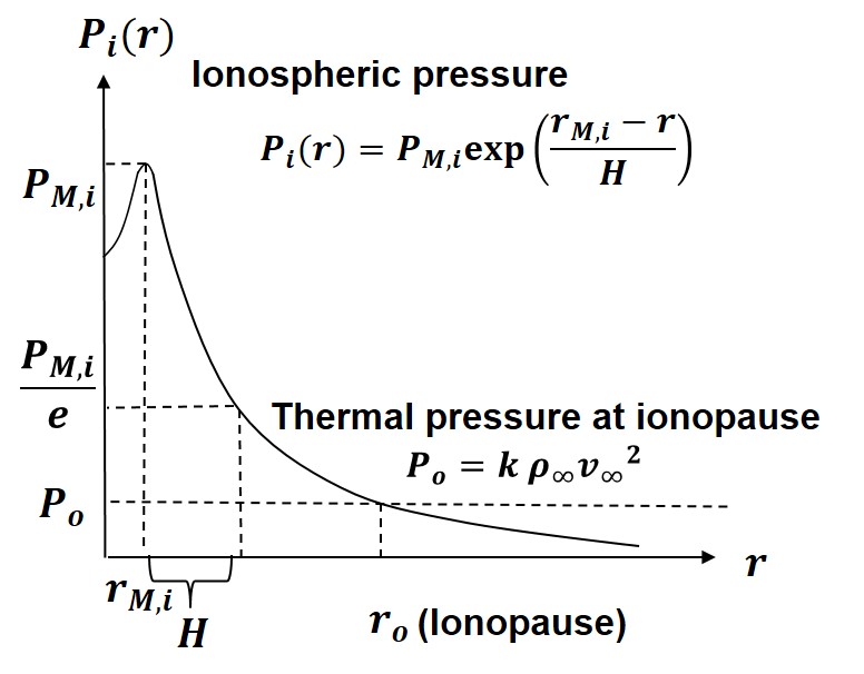
Figure 6: The schematic of the ionopause, where the ionsperic pressure is equal to solar wind thermal pressure.

By solving Eq. 15 with the expression of the thermal pressure at the both side of the ionopause (Eq. 11 and Eq. 13), the formula of the nose position of the bow shock $r_{o}$ can be derived as

$$r_{o}=r_{M,i}+H\ {\rm ln}(\frac{P_{M,i}}{k\rho_{\infty}v_{\infty}^{2}}).$$ (16)

The derived equation of the nose position (Eq. 16) of the ionopause is reasonable: the shorter the scale height $H$ or the larger the dynamic pressure of the solar wind $\rho_{\infty}v_{\infty}^{2}$, then ionopause closer to planet surface.

2.3.3 Radius of curvature at ionopause nose $R_{o}$

In this section, we analytically calculate the radius of curvature at ionopause nose $R_{o}$ by solving the ionopause profile equation near the ionopause nose. Since the ionopause is symmetric at x-axis, the ionopause profile can be expressed as $x=x(y)$ . We do the Taylor expansion at $y=0$ of the ionopause profile $x=x(y)$, then we can get the equation of the ionopause profile at the vicinity of the ionopause nose

$$x(y)=x(0)+(y-0)\,x^{\prime}(0)+\frac{1}{2}(y-0)^{2}x"(0)+...$$ (17)

Note that on the ionopause profile, $x(0)=r_{o}$ and $x^{\prime}(0)=0$. Furthermore, by the definition of the radius of curvature $R(y)=|\frac{(1+x^{\prime}(y))^{3/2}}{x"(y)}|$, the radius of curvature at ionopause nose ($y=0$) can be written as $R_{o}=-1/x"(0)$. Thus, the equation of the ionopause profile near the ionopause nose can be reduced to a quadratic equation

$$x=r_{o}-\frac{1}{2R_{o}}y^{2}.$$ (18)

Here we neglect the third and higher order term of the Taylor expansion.

The whole ionopause profile can be determined by the thermal pressure continuity at the ionopause according to tangential discontinuity, that is, the thermal pressure is equal at the outer side and the inner side of the ionopause.

$$k\rho_{\infty}v_{\infty}^{2}\,{\rm cos^{2}}\psi=P_{i}(r),$$ (19)

where $\psi$ is the angle between $v_{\infty}$ and the normal to ionopause, which is shown in Fig. 7.

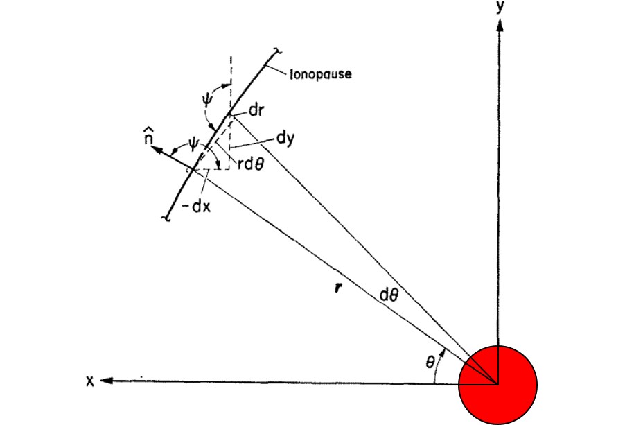
Figure 7: Element of the ionopause and the coordinate. Modified figure from Ref. [1].

The left hand side of the equation is the thermal pressure approximated at the outer side of the ionopause deviated from the nose position and the right hand side is the ionospheric pressure we introduced in section 2.3.1. Since $k\rho_{\infty}v_{\infty}^{2}$ is the ionospheric pressure at the ionopause nose $P_{i}(r_{o})$, the equation of the ionopause profile (Eq.19) can be reduced to

$$P_{i}(r_{o})\,{\rm cos^{2}}\psi=P_{i}(r).$$ (20)

By the geometric relation, $cos^{2}\psi$ can be expressed as

$$cos^{2}\psi=\left(\frac{dy}{ds}\right)^{2}=\frac{\left(r\,d\theta\>{\rm cos}\theta+dr\,{\rm sin}\theta\right)^{2}}{dr^{2}+(r\,d\theta)^{2}}.$$ (21)

We substitute the cosine relation in Eq.21 into the pressure continuity equation at the ionopause (Eq.20), we get

$$P_{i}(r_{o})\frac{\left({\rm cos}\theta+(\frac{dr}{r\,d\theta})\,{\rm sin}\theta\right)^{2}}{\left(\frac{dr}{r\,d\theta}\right)^{2}+1}=P_{i}(r).$$ (22)

Then we solve for $dr/r\>d\theta$ to obtain

$$\frac{dr}{r\,d\theta}=\frac{-P_{i}(r_{o})\,{\rm sin}2\theta+2\sqrt{P_{i}(r)P_{i}(r_{o})-P_{i}^{2}(r)}}{2(P_{i}(r_{o}){\rm sin^{2}}\theta-P_{i}(r))}.$$ (23)

This is the differential equation for the ionopause profile, which can be solved numerically[1] with the initial condition $r\left(\theta=0\right)=r_{o}$. Note that the ionopause is symmetric about the $x=0$ axis ($\theta=0$), so the first-order derivative at the ionopause nose is zero, that is,

$$\frac{1}{r(0)}\frac{dr}{d\theta}(0)=\frac{1}{r_{o}}\frac{dr}{d\theta}(0)=0.$$ (24)

In the second term of the numerator in the ionopause profile differential equation (Eq.23), it contains a square root. The value of the quantity inside the square root must be equal or larger than zero, or the square root term will become imaginary, which is physically unallowable. So, we can get

$$P_{i}(r)P_{i}(r_{o})-P_{i}^{2}(r)\geq 0,$$ (25)

where $P_{i}(r)$ is the ionospheric pressure exponentially decaying outward because of hydrostatic equilibrium. Then we can obtain that the ionopause profile must follow the condition

$$r\geq r_{o}.$$ (26)

The equality occurs at the ionopause nose.

For our purpose of deriving the radius of curvature at the ionopause nose, we only have to focus on the vicinity of the ionopause nose, i.e., the region $\theta\rightarrow 0$ and $r\rightarrow r_{o}$. Furthermore, at the ionospause nose, $dr/rd\theta$ can be approximated by $dx/dy.$ The differential equation for the ionopause profile (Eq. 23) at the vicinity of the ionopause nose can be simplified to

$$\frac{dx}{dy} =-\sqrt{\frac{P_{i}(r_{o})}{P_{i}(r)}-1}$$

$$=-\sqrt{\frac{P_{i}(r_{o})}{P_{i}(r)}}\sqrt{1-\frac{P_{i}(r)}{P_{i}(r_{o})}}$$

$$\simeq-\sqrt{1-\frac{P_{i}(r)}{P_{i}(r_{o})}}.$$ (27)

Now we express $P_{i}(r)$ in Taylor series at $r=r_{o}$, then the right hand side of the Eq. 27 can be rewritten as

$$-\sqrt{1-\frac{P_{i}(r)}{P_{i}(r_{o})}} =-\sqrt{-(r-r_{o})\frac{P_{i}^{\prime}(r_{o})}{P_{i}(r_{o})}-\frac{1}{2}(r-r_{o})^{2}\frac{P_{i}"(r_{o})}{P_{i}(r_{o})}-...}$$

$$=-\sqrt{-(r-r_{o})\frac{P_{i}^{\prime}(r_{o})}{P_{i}(r_{o})}}\sqrt{1+\frac{1}{2}(r-r_{o})\frac{P_{i}"(r_{o})}{P_{i}^{\prime}(r_{o})}+...}$$

$$\simeq-\sqrt{-(r-r_{o})\frac{P_{i}^{\prime}(r_{o})}{P_{i}(r_{o})}}\left(1+\frac{1}{4}(r-r_{o})\frac{P_{i}"(r_{o})}{P_{i}^{\prime}(r_{o})}+...\right).$$ (28)

Thus, now the differential equation for the ionopause profile near the ionopause nose is

$$\frac{dx}{dy}=-\sqrt{-(r-r_{o})\frac{P_{i}^{\prime}(r_{o})}{P_{i}(r_{o})}}\left(1+\frac{1}{4}(r-r_{o})\frac{P_{i}"(r_{o})}{P_{i}^{\prime}(r_{o})}+...\right)$$ (29)

Also, by $x\rightarrow r_{o}$and $y\rightarrow 0$ at the vicinity of the ionopause nose, $r-r_{o}$ can be approximated by

$$r-r_{o} =\sqrt{x^{2}+y^{2}}-r_{o}$$

$$=\sqrt{\left[r_{o}+\left(x-r_{o}\right)\right]^{2}+y^{2}}-r_{o}$$

$$=\sqrt{r_{o}^{2}+2\,r_{o}(x-r_{o})+(x-r_{o})^{2}+y^{2}}-r_{o}$$ (30)

$$=r_{o}\sqrt{1+2\,\frac{x-r_{o}}{r_{o}}+\frac{\left(x-r_{o}\right)^{2}}{r_{o}^{2}}+\frac{y^{2}}{r_{o}^{2}}}-r_{o}$$

$$\simeq r_{o}(1+\frac{x-r_{o}}{r_{o}}+\frac{\left(x-r_{o}\right)^{2}}{2\,r_{o}^{2}}+\frac{y^{2}}{2\,r_{o}^{2}})-r_{o}$$ (31)

$$=x-r_{o}+\frac{\left(x-r_{o}\right)^{2}}{2\,r_{o}}+\frac{y^{2}}{2\,r_{o}}.$$ (32)

By substituting the equation of the ionopause profile near the ionopause nose (Eq.18) in to Eq.32, we get

$$r-r_{o} =-\frac{1}{2R_{o}}y^{2}+\frac{\left(-\frac{1}{2R_{o}}y^{2}\right)^{2}}{2\,r_{o}}+\frac{y^{2}}{2\,r_{o}}$$ (33)

$$\simeq\frac{y}{2}^{2}\left(\frac{1}{r_{o}}-\frac{1}{R_{o}}\right)$$ (34)

In Eq.33, the second term at the right hand side is negligible as $y\rightarrow 0$ since it is of the order $y^{4}$ and the other two terms are of the order $y^{2}$.

We plug the $r-r_{o}$ relation (Eq. 34) into the differential equation of the ionopause profile (Eq. 29), then integrate the differential equation

$$\sideset{}{{}_{r_{o}}^{x}}{\int}dx=\sideset{-}{{}_{0}^{y}}{\int}dy\,\sqrt{\frac{-1}{2}\frac{P_{i}^{\prime}(r_{o})}{P_{i}(r_{o})}\left(\frac{1}{r_{o}}-\frac{1}{R_{o}}\right)}\left(y+\frac{1}{8}\left(\frac{1}{r_{o}}-\frac{1}{R_{o}}\right)\frac{P_{i}^{\prime\prime}(r_{o})}{P_{i}^{\prime}(r_{o})}\,y^{3}+...\right).$$ (35)

Therefore we obtain the formula of the ionopause profile at the vicinity of the ionopause:

$$x=r_{o}-\sqrt{-\frac{P_{i}^{\prime}(r_{o})}{2P_{i}(r_{o})}\left(\frac{1}{r_{o}}-\frac{1}{R_{o}}\right)}\left(\frac{y^{2}}{2}+\frac{1}{32}\left(\frac{1}{r_{o}}-\frac{1}{R_{o}}\right)\frac{P_{i}^{\prime\prime}(r_{o})}{P_{i}^{\prime}(r_{o})}\,y^{4}+...\right).$$ (36)

By comparing Eq. 36 and Eq. 18, finally, we get the equation of the radius of curvature at the ionopause nose

$$R_{o}=\sqrt{-\frac{2P_{i}(r_{o})}{P_{i}^{\prime}(r_{o})}\frac{R_{o}r_{o}}{R_{o}-r_{o}}}.$$ (37)

Eq.37 can be rearranged as a quadratic equation

$$R_{o}^{2}-r_{o}\,R_{o}-\sqrt{-\frac{2P_{i}(r_{o})}{P_{i}^{\prime}(r_{o})}}\,r_{o}=0.$$ (38)

Then we solve it and get

$$R_{o}=\frac{r_{o}\pm\sqrt{r_{o}^{2}+4\,\sqrt{-\frac{2P_{i}(r_{o})}{P_{i}^{\prime}(r_{o})}}\,r_{o}}}{2}.$$ (39)

We take the plus sign in the nominator since $R_{o}$ will be negative if we take the minus sign, which is not physically allowable. Thus, we obtain the expression of the radius of curvature at the ionopause nose

$$R_{o}=\frac{r_{o}+\sqrt{r_{o}^{2}+4\,\sqrt{-\frac{2P_{i}(r_{o})}{P_{i}^{\prime}(r_{o})}}\,r_{o}}}{2}.$$ (40)

With the ionospheric pressure $P_{i}(r)$ of the form in Eq. 11, the radius of curvature at the ionopause nose can be expressed as

$$R_{o}=\frac{r_{o}+\sqrt{r_{o}^{2}+8\,H\,r_{o}}}{2},$$ (41)

where $H$ is the scale height of the ionosphere. The expression of the radius of curvature at the ionopause nose from our calculation is the same as that from the Table A1 in Verigin et al. (2003) [10]. Thus, by plugging Eq.41 into Eq.18, we can get the ionopause profile near the ionopause nose

$$x=r_{o}-\frac{1}{r_{o}+\sqrt{r_{o}^{2}+8\,H\,r_{o}}}\,y^{2}.$$ (42)

In the derivation of the radius of curvature at the ionopause nose and the ionopause profile near the ionopause nose, we made many assumptions to get it. We have shown that the assumption we made above is all valid by verifying our analytical results with the simulation results, which will be given in Section 3.1.

This equation of the radius of the curvature at the ionopause (Eq.41) tells that

$$R_{o}\geq r_{o}.$$ (43)

The equality occurs as the ionospheric scale height $H$ is close to zero. By the equation of the ionopause nose location (Eq.16), we get that $r_{o}$ is equal to $r_{M,i}$ when $H$ is zero. Combining the above relation, we found that

$$R_{o}\rightarrow r_{M,i}\;{\rm as\;H\rightarrow 0}.$$ (44)

This relation means that if the ionospheric pressure decreases very sharply outward, the radius of the ionopause nose is about the distance between the location of the ionospheric peak pressure and the planet center. Furthermore, we can observe that $R_{o}$ is smaller as the dynamic pressure of the solar wind is larger since $r_{o}$ is smaller. These results are physically reasonable.

2.4 Bow shock standoff distance $\Delta$

The standoff distance of the bow shock $\Delta$ is determined by the empirical model [4, 6, 10, 20]. This empirical model is supported by gasdynamics experiment and observations of the flow past the planets[9]. The standoff distance is expressed by the empirical model

$$\frac{\Delta}{R_{o}}=\alpha\frac{\rho_{\infty}}{\rho_{s}},$$ (45)

where $\rho_{\infty}$and $\rho_{s}$ are the mass density before and after shock, respectively and

$$\alpha\approx 0.87$$

is the empirical coefficient from [4, 10]. The bow shock nose is farther from the obstacle as the radius of curvature of the obstacle nose is larger (Fig. 8). Bow shock can touch the obstacle only when the leading end of the obstacle is pointed.

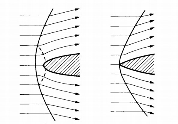
Figure 8: Schematic of the detached shock. Courtesy of [18]

The density ratio across the shock is related to solar wind Mach number and the specific heat ratio

$$\frac{\rho_{\infty}}{\rho_{s}}=\frac{(\gamma-1)M_{\infty}^{2}+2}{(\gamma+1)M_{\infty}^{2}}.$$ (46)

Thus, in the condition of the solar wind Mach number much larger than 1, the standoff distance can be expressed as

$$\Delta=\alpha\ R_{o}\epsilon,\quad M_{\infty}\gg 1,$$ (47)

where $\epsilon=\frac{\gamma-1}{\gamma+1}$. By substituting the Eq. 41 into Eq. 47, we get

$$\Delta =\alpha\epsilon\frac{r_{o}+\sqrt{r_{o}^{2}+8\,H\,r_{o}}}{2},\quad M_{\infty}\gg 1,$$ (48)

$$=\frac{1}{2}\,r_{o}\,\alpha\,\epsilon\left(1+\sqrt{1+8\,H/r_{o}}\right),\quad M_{\infty}\gg 1.$$

According to this relation, we can obtain the value of the standoff distance if we have the ratio of $H$ (scale height of the ionosphere) to $r_{o}$ (the distance between ionopause and the center of the planet).

2.5 The formula of the bow shock nose location

Thus, combining the results above, the shock nose location can be written as

$$r_{s} =r_{o}+\Delta,$$ (49)

$$=r_{o}+\frac{1}{2}\,\alpha\,\epsilon\left(r_{o}+\sqrt{r_{o}^{2}+8\,H\,r_{o}}\right),\quad M_{\infty}\gg 1,$$

where

$$r_{o}=r_{M,i}+H\ {\rm ln}(\frac{P_{M,i}}{k\rho_{\infty}v_{\infty}^{2}}),$$ (50)

, scale height $H=k_{B}T/(mg)$ and $\epsilon=\frac{\gamma-1}{\gamma+1}$.

Note that this equation is only valid for the sonic Mach number of the solar wind much larger than 1. As we can see in the shock nose equation (Eq. 49): the shorter the scale height $H$ or the larger the dynamic pressure of the solar wind $\rho_{\infty}v_{\infty}^{2}$, bow shock nose is closer to the planet. This result is reasonable and intuitive.

3 Comparison with the numerical simulation and spacecraft measurement results

The comparison of our formula of the bow shock location with the numerical simulation and the spacecraft measurement results is given in this section.

3.1 Verification of the analytical form of the radius of curvature by simulation

In this subsection, we verify the analytical results of the radius of curvature from the Section 2.3.3 by the numerical simulation. In our calculation, we analytically solve the differential equation of the ionopause profile (Eq. 23) near the ionopause nose ($\theta\rightarrow 0$) with the initial condition $r\left(\theta=0\right)=r_{o}$ to the get the equation of the ionopause profile near the ionopause nose (Eq. 42). The radius of curvature at the ionopause nose is also obtained in Eq. 41. In the derivation of the equation of the ionopause profile near the ionopause nose and the radius of curvature at the ionopause nose, we made many assumptions, so we will verify that the assumptions are valid by numerical simulation.

We use the function NDSolve in the software Mathematica to solve the differential equation of the ionopause profile (Eq. 23) to get the ionopause profile $r=r(\theta)$. We first compare the numerical result with our analytical result of the ionopause profile near the ionopause nose (Eq. 42). Fig. 9 shows the comparison of the ionopause profile from analytical theory and numerical simulation. We can observe that, from both the simulation and analytical results, the ionopause follows the rule that

$$r\geq r_{o},$$ (51)

which we show in the section 2.3.3. Also, we can see that the ionopause profile from analytical theory and numerical simulation match well near the nose position ($y\rightarrow 0$), which is reasonable since the analytical result is calculated under the approximation that $\theta\rightarrow 0$ in polar coordinate or $y\rightarrow 0$ in Cartesian coordinate.

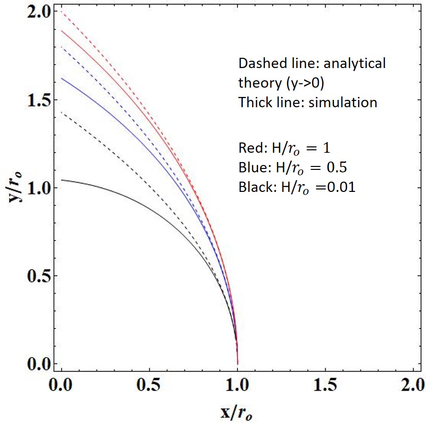
Figure 9: Ionopause profile calculated from analytical theory (Eq. 42) and numerical simulation. The analytical results is calculated under the approximation that $\theta\rightarrow 0$ in polar coordinate or $y\rightarrow 0$ in Cartesian coordinate.

We then compare the numerical results with our analytical result of the radius of curvature at the ionopause nose (Eq. 41). In the numerical simulation, we numerically solve the differential equation of the ionopause profile (Eq. 23) to get the ionopause profile $r=r(\theta)$ using the function NDSolve in Mathematica and then calculate the radius of curvature at $\theta=0$ in polar coordinate using the formula

$$R(\theta)=\frac{\left(r^{2}(\theta)+r^{\prime 2}(\theta)\right)^{3/2}}{|r^{2}(\theta)+2\,r^{\prime 2}(\theta)-r(\theta)r^{\prime\prime}(\theta)|}.$$ (52)

The comparison results are shown in Fig. 10. We can see that the difference between analytical and numerical results is smaller than 1 percent. Thus, our analytical form of the radius of curvature at the ionopause nose (Eq. 41) is verified. And we can say that the assumptions we made in the derivation are valid.

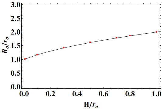
Figure 10: Radius of curvature at the ionopause nose from analytical theory (Eq. 41) and numerical simulation. The thick line is the analytical theory (Eq. 41) and the red dots are simulation results. The cases with $H/r_{o}=0.01,\,0.1,\,0.3,\,0.5,\,0.7,\,0.8,\,1.0$ are considered.

3.2 Comparison with hydrodynamics simulation

We now want to compare our formula of the bow shock nose with the simulation and spacecraft measurement results. Our derived formula of the bow shock location is $r_{s}=r_{o}+\Delta$ and the standoff distance is

$$\frac{\Delta}{r_{o}}=\frac{1}{2}\,\alpha\,\epsilon\left(1+\sqrt{1+8\,H/r_{o}}\right),\quad M_{\infty}\gg 1,$$ (53)

where $\epsilon=\frac{\gamma-1}{\gamma+1}$. In Fig. 11, we compare our formula of the standoff distance with the nonlinear gasdynamics simulation result for the bow shock profile, which is referred to the paper by Spreiter et al., 1970[1].

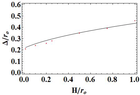
Figure 11: Comparison of the derived standoff distance formula (Eq. 53) with the gasdynamics simulation results from Spreiter et al., 1970[1]. The red dots are the simulation results; the black line is Eq. 53. The cases with $H/r_{o}=0.01,\,0.1,\,0.2,\,0.25,\,0.5,\,0.75,\,1.0$ are considered.

As we can observe in the comparison, our derived formula (Eq. 53) and the simulation results match well and both show that the standoff distance becomes larger with the increasing scale heights of the ionosphere. We can conclude that the theory is validated by the simulation results. Note that this formula of the bow shock standoff distance is only applied for the solar wind interacting with the unmangetized planet and the Mach number of the solar wind solar wind must be much larger than 1. The other assumption in this theory is that the ionosphere of the unmagnetized planet is in hydrostatic condition, resulting in the thermal pressure exponentially decaying outward.

3.3 Comparison with spacecraft measurements in Martian bow shock

We investigate the influence of the shock location from solar parameters, which control the $P_{dyn}$ (dynamic pressure of the solar wind), $P_{M,i}$ (peak pressure of the ionosphere), $H=k_{B}T/mg$ (scale height of the ionosphere). Our derived formula of the shock nose location is

$$r_{s}=r_{o}+\frac{1}{2}\,r_{o}\,\alpha\,\epsilon\left(1+\sqrt{1+8\,H/r_{o}}\right),\quad M_{\infty}\gg 1,$$ (54)

where $\epsilon=\frac{\gamma-1}{\gamma+1}$ and

$$r_{o}=r_{M,i}+H\ {\rm ln}(\frac{P_{M,i}}{k\,P_{dyn}}).$$ (55)

According to the spacecraft measurement[3] (Fig. 3), the measurement data shows that the Martian bow shock location increases linearly with the increasing EUV flux, i.e.,

$$r_{s}\propto 0.11\,l_{EUV},$$ (56)

but it reduces through a power law relationship with solar wind dynamic pressure, i.e.,

$$r_{s}\propto p_{dyn}^{-0.02}.$$ (57)

We can observe that our relation in Eq. 54 and the spacecraft measurement results in Eq. 57 both shows that the increasing solar EUV flux and decreasing solar wind dynamic pressure will increase the bow shock location. The increasing solar EUV flux will cause the $P_{M,i}$ (peak pressure of the ionosphere) increase via increasing the ionization rate. Furthermore, the increasing solar EUV flux will let the temperature increase, i.e., a larger scale height $H$. Since the dynamics pressure $P_{dyn}$ term is in the logarithm in our relation in Eq. 54, we suggest that the variation of dynamics pressure has less impact on the shock location than the EUV flux, which controls the scale height $H$ and ionospheric peak pressure $P_{M,i}$. Thus, our derived formula is qualitatively consistent with the spacecraft measurement results that the shock nose location is more sensitive to the solar EUV flux than solar wind dynamics pressure.

The power-law dependence of Martian bow shock location on solar wind dynamics pressure according to spacecraft measurement results (Eq. 57) can be rewritten

$$\frac{d\,r_{s}}{r_{s}}=-C\,\frac{d\,P_{dyn}}{P_{dyn}}.$$ (58)

where

$$C=0.02.$$

Now we derive the mathematical expression of the $C$ using our formula of the shock nose location (Eq. 54) and then compare it with the spacecraft measurement results. In the Martian condition, the scale height $H$ is much shorter than the distance between the Martian ionopause nose and the Mars center $r_{o}$, so the square root term in our formula of the bow shock location (Eq. 54) can be expanded, then it can be reduced to

$$r_{s} \simeq r_{o}+\frac{1}{2}\,r_{o}\,\alpha\,\epsilon\,(1+1+4\frac{H}{r_{o}}),$$ (59)

$$=r_{o}(1+\alpha\,\epsilon)+2\,\alpha\,\epsilon\,H,$$ (60)

$$=(1+\alpha\,\epsilon)\,r_{M,i}+(1+\alpha\,\epsilon)\,H\,{\rm ln}\left(\frac{P_{M,i}}{k\,P_{dyn}}\right)+2\,\alpha\,\epsilon\,H.$$ (61)

We are interested in the bow shock location $r_{s}$dependence on $H,\;P_{M,i},\;P_{dyn}$. The total variation of the bow shock location $r_{s}$ is written as

$$d\,r_{s}=\left[\left(1+\alpha\,\epsilon\right){\rm ln}\left(\frac{P_{M,i}}{k\,P_{dyn}}\right)+2\,\alpha\,\epsilon\right]\,d\,H+\left[\left(1+\alpha\,\epsilon\right)\,\frac{H}{P_{M,i}}\right]\,d\,P_{M,i}+\left[-\left(1+\alpha\,\epsilon\right)\,\frac{H}{P_{dyn}}\right]\,d\,P_{dyn}.$$ (62)

The bow shock location $r_{s}$ dependence on the solar wind dynamics pressure $P_{dyn}$ is

$$\frac{d\,r_{s}}{r_{s}}=-(1+\alpha\,\epsilon)\,\frac{H}{r_{s}}\,\frac{d\,P_{dyn}}{P_{dyn}},$$ (63)

where we assume the $H\;{\rm and}\;P_{M,i}$ are fixed. Thus, we get the expression of $C$ as

$$C=(1+\alpha\,\epsilon)\,\frac{H}{r_{s}}.$$ (64)

$C$ is approximately the ratio between ionospheric scale length and the distance between bow shock nose location and the planet center. According to spacecraft measurement results in the Martian environment [3], the ionospheric scale height $H$ is about 100 km and the distance between the Martian bow shock location between the Mars center is about 2.5 Mars radius (8473 km). Also, with $\alpha=0.87$ and $\epsilon=0.25$, the value of $C$ calculated from Eq. 64 is 0.014, which is at the same order of the results from spacecraft measurement results ($C=0.02$). Thus, in terms of the bow shock location dependence on the solar wind dynamics pressure, our formula is verified by the spacecraft measurement results. This formula can be used for the future spacecraft measurement prediction.

4 Conclusion

It is not well understood how the solar parameters, such as solar wind dynamics pressure, solar wind EUV flux and ionospheric pressure, influence the location of the Martian (unmagnetized planet) bow shock. The location of the bow shock produced from the solar wind interacting with the unmagnetized planet has been theoretically investigated. The formula for the location of the bow shock produced from the solar wind interacting with the unmagnetized planet is presented. The bow shock location is the sum of the ionopause location and standoff distance. The whole calculation is based on the gasdynamics formulation since the magnetic effect can be neglected in space environment for our purpose. We determine the ionopause nose location using thermal pressure continuity according to tangential discontinuity. The standoff distance of the bow shock produced by the supersonic plasma jet with sonic Mach number much larger than 1 past the obstacle is given in the empirical formula that the standoff distance is proportional to the radius of curvature at obstacle leading end. The formula of the shock nose position was derived and showed that the shock nose location increases with the increasing scale height of ionosphere, the decreasing dynamic pressure of the solar wind and the increasing peak pressure of the ionosphere. Furthermore, we derived the equation of the ionopause profile around the nose. Our derived theory is consistent with the numerical simulation. The derived analytical form of the radius of curvature at the obstacle leading end is verified by the numerical simulation. Also, the derived formula of the bow shock location for the unmagnetized planet is consistent with the results from the gasdynamics simulations.

Furthermore, we derived that the relation between the unmagnetized planet bow shock location and solar wind dynamics pressure, which is $r_{s}\propto p_{dyn}^{-C},$ where the constant $C$ is roughly the ratio between ionospheric scale length and the distance between bow shock nose location and the The constant $C$ calculated from the Martian parameter with our formula is at the same order as the results from the spacecraft measurements by Mars Express[14]. Also, our derived formula is qualitatively consistent with the spacecraft measurement results that the shock nose location is more sensitive to the solar EUV flux than solar wind dynamics pressure.

Since our model only provide the relation between bow shock location and the solar wind dynamics pressure, in order to have a more thorough comparison of our theory with the measurement results, we have to study how the solar EUV flux controls the ionospheric pressure, which is related to the photoionization from EUV radiation. On the other hand, throughout this work, we neglect the effect of the magnetic field for simplicity. In fact, Mars has some local magnetic field, which can influence the bow shock nose location. The magnetic field also influences the formation mechanisms of the bow shock and the ionopause. In the realistic condition, the interaction between the interplanetary magnetic field and the ionosphere will generate the “induced magnetosphere” and “magnetic pile-up boundary”. Furthermore, the magnetic draping effect will occur. Although the detailed study of how important the interplanetary magnetic field plays the role on controlling the bow shock location is yet to be done, our model with no magnetic field effect can now accurately predict the bow shock nose location and its relationship with the solar wind dynamics pressure, which has been verified by both numerical simulation and spacecraft measurement results.

5 Acknowledgment

I.L.Yeh acknowledges support through MOST grant No. and the helpful discussion with Frank C.Z. Cheng and Ling-Hsiao Lyu. I.L. Yeh did all the calculation and simulation and wrote the paper draft. P.Y. Chang came up with this project and reviewed the draft. Sunny W.Y. Tam reviewed the draft and provided the insights on the comparison with the theory and spacecraft measurement results.

References

- [1] John R Spreiter, Audrey L Summers, and Arthur W Rizzi. Solar wind flow past nonmagnetic planets—venus and mars. Planetary and Space Science, 18(9):1281–1299, 1970.
- [2] Christopher T. Russell Margaret G. Kivelson, editor. Introduction to space physics. Cambridge university press, 1995.
- [3] Marissa F Vogt, Paul Withers, Paul R Mahaffy, Mehdi Benna, Meredith K Elrod, Jasper S Halekas, John EP Connerney, Jared R Espley, David L Mitchell, Christian Mazelle, et al. Ionopause-like density gradients in the martian ionosphere: A first look with maven. Geophysical Research Letters, 42(21):8885–8893, 2015.
- [4] MH Farris and CT Russell. Determining the standoff distance of the bow shock: Mach number dependence and use of models. Journal of Geophysical Research: Space Physics, 99(A9):17681–17689, 1994.
- [5] JG Trotignon, C Mazelle, C Bertucci, and MH Acuna. Martian shock and magnetic pile-up boundary positions and shapes determined from the phobos 2 and mars global surveyor data sets. Planetary and Space Science, 54(4):357–369, 2006.
- [6] John R Spreiter, Audrey L Summers, and Alberta Y Alksne. Hydromagnetic flow around the magnetosphere. Planetary and Space Science, 14(3):223–253, 1966.
- [7] John R Spreiter and SS Stahara. The location of planetary bow shocks: A critical overview of theory and observations. Advances in Space Research, 15(8-9):433–449, 1995.
- [8] James A Slavin and Robert E Holzer. Solar wind flow about the terrestrial planets 1. modeling bow shock position and shape. Journal of Geophysical Research: Space Physics, 86(A13):11401–11418, 1981.
- [9] JA Slavin, RE Holzer, JR Spreiter, SS Stahara, and DS Chaussee. Solar wind flow about the terrestrial planets: 2. comparison with gas dynamic theory and implications for solar-planetary interactions. Journal of Geophysical Research: Space Physics, 88(A1):19–35, 1983.
- [10] M Verigin, J Slavin, A Szabo, T Gombosi, G Kotova, O Plochova, K Szegö, M Tátrallyay, K Kabin, and F Shugaev. Planetary bow shocks: Gasdynamic analytic approach. Journal of Geophysical Research: Space Physics, 108(A8), 2003.
- [11] John R Spreiter and Stephen S Stahara. A new predictive model for determining solar wind-terrestrial planet interactions. Journal of Geophysical Research: Space Physics, 85(A12):6769–6777, 1980.
- [12] John R Spreiter and Stephen S Stahara. Computer modeling of solar wind interaction with venus and mars. Washington DC American Geophysical Union Geophysical Monograph Series, 66:345–383, 1992.
- [13] Yingjuan Ma, Andrew F Nagy, Kenneth C Hansen, Darren L DeZeeuw, Tamas I Gombosi, and KG Powell. Three-dimensional multispecies mhd studies of the solar wind interaction with mars in the presence of crustal fields. Journal of Geophysical Research: Space Physics, 107(A10):SMP–6, 2002.
- [14] Benjamin Edward Stanley Hall, Mark Lester, Beatriz Sánchez-Cano, Jonathan D Nichols, David J Andrews, Niklas JT Edberg, Hermann J Opgenoorth, Markus Fränz, M Holmström, Robin Ramstad, et al. Annual variations in the martian bow shock location as observed by the mars express mission. Journal of Geophysical Research: Space Physics, 121(11):11–474, 2016.
- [15] D Vignes, MH Acuña, JEP Connerney, DH Crider, H Reme, and C Mazelle. Factors controlling the location of the bow shock at mars. Geophysical research letters, 29(9):42–1, 2002.
- [16] Niklas JT Edberg, M Lester, SWH Cowley, DA Brain, M Fränz, and S Barabash. Magnetosonic mach number effect of the position of the bow shock at mars in comparison to venus. Journal of Geophysical Research: Space Physics, 115(A7), 2010.
- [17] NJT Edberg, M Lester, SWH Cowley, and AI Eriksson. Statistical analysis of the location of the martian magnetic pileup boundary and bow shock and the influence of crustal magnetic fields. Journal of Geophysical Research: Space Physics, 113(A8), 2008.
- [18] Lev Davidovich Landau and EM Lifshiëtís. Fluid mechanics. Butterworth-Heinemann,, 1987.
- [19] Ya B Zel’Dovich and Yu P Raizer. Physics of shock waves and high-temperature hydrodynamic phenomena. Courier Corporation, 2012.
- [20] Alvin Seiff. Recent information on hypersonic flow fields. NASA Special Publication, 24:19, 1962.