Abstract

The present paper addresses the issue of choosing an optimal dynamic reinsurance policy, which is state-dependent, for an insurance company that operates under multiple insurance business lines. For each line, the Cramer-Landberg model is adopted for the risk process and one of the contracts such as Proportional reinsurance, excess-of-loss reinsurance (XL) and limited XL reinsurance (LXL) is intended for transferring a portion of the risk to reinsurance. In the optimization method used in this paper, the survival function is maximized relative to the dynamic reinsurance strategies. The optimal survival function is characterized as the unique nondecreasing viscosity solution of the associated Hamilton-Jacobi-‌‌‌‌‌‌Bellman equation (HJB) equation with limit one at infinity. The finite difference method (FDM) has been utilized for the numerical solution of the optimal survival function and optimal dynamic reinsurance strategies and the proof for the convergence of the numerical solution to the survival probability function is provided. The findings of this article provide insights for the insurance companies as such that based upon the lines in which they are operating, they can choose a vector of the optimal dynamic reinsurance strategies and consequently transfer some part of their risks to several reinsurers. Using numerical examples, the significance of the elicited results in reducing the probability of ruin is demonstrated in comparison with the previous findings.

Keywords: Cramer-lundberg process; Optimal reinsurance; Hamilton-Jacobi-Bellman equation; Viscosity solution; Dynamic programming principle.

1 Introduction

An effective way for an insurance firm to manage its risk is to buy reinsurance. According to the reinsurance contract, some parts of the claim are shared with the reinsurer, and against, the insurance firm pays a part of its income premium to the reinsurance. Determination of the optimal reinsurance contracts has been discussed extensively in the literature. Dynamic proportional reinsurance in the classical risk model for the minimization of the ruin probability was first studied by Schmidli (2001). Hipp & Vogt (2003) utilized the concept of dynamic excess of loss reinsurance to extend the Schimidli approach. Schmidli et al. (2002) have suggested the optimal investment and reinsurance strategies to minimise the ruin probability and have concluded that the investment and reinsurance decrease the ruin probability for larger initial surplus under the Pareto claim sizes. In this direction, Taksar & Markussen (2003) and Schmidli (2004) developed the above approach to the diffusion model. Subsequently, Irgens & Paulsen (2004) discussed the maximization of the expected utility of the asset of an insurance company under the reinsurance and investment constraints in a diffusion classical risk model. A general presentation on ruin probability minimization by means of reinsurance in a classical and diffusion risk models can be found in Schmidli (2007). Some additional results with a focus on non-proportional reinsurance contracts are given in Hipp & Taksar (2010). Recently, Cani & Thonhauser (2017) studied a dynamic reinsurance problem obtained from an economical valuation criterion in risk theory introduced by Højgaard & Taksar (1998a, b).

In this paper, we assume that the insurance company produces multiple types of coverage, where customers may purchase different types of insurance policies (such as fire, health, vehicle, etc.). Due to the different risk processes in different lines, it is reasonable that the insurance companies use several reinsurances to share their risk. For instance, it is possible for an insurance company to purchase a proportional reinsurance in one line and an excess-of-loss reinsurance in another line or buy one type of excess-of-loss in one line and a different type of excess-of-loss insurance in another line. The survival function, in this paper, is considered as the objective function, and the vector of reinsurance strategies is obtained in such a way that the objective function is maximized; therefore, the results presented in Azcue & Muler (2014), which use a dynamic reinsurance strategy for transferring risk to reinsurers, have been generalized in such a way that the insurer uses the vector of dynamic reinsurance strategies to transfer risk to several reinsurers.

In the second section of the paper, a brief introduction of the model with the presence of the reinsurer and the statement of the problem are provided. In the third section, the main results and in the fourth section numerical examples are presented.

2 Model formulation

In the classical Cramer-Lundberg process, the reserve $X_{t}$ of an insurance company can be described by

$$X_{t}=x+pt-\sum_{i=1}^{N_{t}}U_{i}$$ (2.1)

where $N_{t}$ is a Poisson process with claim arrival intensity $\beta>0$ and the claims size $U_{i}$ are i.i.d random variables with distribution $F$. The premium rate $p$ is calculated using the expected value principle with relative safety loading $\eta>0$; that is, $p=(1+\eta)\beta\mu$.the limitation of this model is the assumption that insurers produce only one type of insurance, but in practice, most insurers produce different types of coverage. (e.g. automobile insurance, fire insurance, workers’ compensation insurance, etc.). The idea for modeling the surplus process for a company that produces multiple types of coverage is as follows: consider the process $X_{t}=(X_{t}^{1},\cdots,X_{t}^{n})$ defined as;

$$X_{t}^{(k)}=p_{k}t-\sum_{i=1}^{N_{t}^{(k)}}U_{i}^{(k)},\qquad\qquad\qquad k=1,\cdots,n$$ (2.2)

where $N_{t}^{(k)}$ is a Poisson process with claim arrival intensity $\beta_{k}>0$ and the claims size $U_{i}^{(k)}$’s are i.i.d random variables with distribution $F_{k}$. Let the risk process of the $k$th line of insurance company be modelled by $X_{t}^{(k)}$. The premium rate $p_{k}$ is calculated using the expected value principle with relative safety loading $\eta>0$; that is, $p_{k}=(1+\eta)\beta_{k}\mu_{k}$. Given an initial surplus $x$, the surplus $Y_{t}$ of the insurance company at time $t$ can be written as $Y_{t}=x+\sum_{k=1}^{n}X_{t}^{(k)}$ and if $X_{t}^{(1)},\cdots,X_{t}^{(n)}$ are independent random variables, then $Y_{t}$ has a compound Poisson distribution, that is,

$$Y_{t}=x+(\sum_{k=1}^{n}p_{k})t-\sum_{i=1}^{N_{t}}U_{i},\qquad\qquad\qquad k=1,\cdots,n$$ (2.3)

where $N_{t}$ is a Poisson process with claim arrival intensity $\beta=\sum_{i=1}^{n}\beta_{i}$ and the claims size $U_{i}$’s are i.i.d random variables with distribution $\sum_{i=1}^{n}\frac{\beta_{i}}{\sum_{i=1}^{n}\beta_{i}}F_{i}$. Let $(\Omega_{k},\Sigma_{k},({{\cal{F}}_{k}}_{t})_{t\geq 0},P_{k})$ be the filtered probability space corresponds to line $k$, then, we can describe filtered probability space model by

$$(\boldsymbol{\Omega},\boldsymbol{\Sigma},(\boldsymbol{{\cal{F}}}_{t})_{t\geq 0},\boldsymbol{P})=(\Omega_{1},\Sigma_{1},({{\cal{F}}_{1}}_{t})_{t\geq 0},P_{1})\times\cdots\times(\Omega_{n},\Sigma_{n},({{\cal{F}}_{n}}_{t})_{t\geq 0},P_{n}).$$ (2.4)

Reinsurance can be an effective way to manage risk by transferring risk from an insurer to a second insurer (referred to as the reinsurer). A reinsurance contract is an agreement between an insurer and a reinsurer under which, claims that arise are shared between the insurer and reinsurer.

Let a Borel measurable function $R:[0,\infty)\longrightarrow[0,\infty)$, called retained loss function, describing the part of the claim that the company pays and satisfies $0\leq R(\alpha)\leq\alpha$. The reinsurance company covers $\alpha-R(\alpha)$), where the size of the claim is $\alpha$. Now assume that in order to reduce the risk exposure of the portfolio, the insurer has the possibility to take reinsurances in a dynamic way for some insurance lines, each of these reinsurances is indexed by $\{1,\cdots,n\}$. We denote by $\boldsymbol{\mathcal{R}}$ the vector $(\mathcal{R}_{1},\cdots,\mathcal{R}_{n})$, in which $\mathcal{R}_{i}$ is the family of retained loss functions associated to the reinsurance policy in $i$’th line, and denote by $\Pi_{x}^{\boldsymbol{R}}$ the set of all control strategies with initial surplus $x\geq 0$. So, the reinsurances control strategy is a collection $\boldsymbol{R}=(\boldsymbol{R}_{t})_{t\geq 0}=({R_{1}}_{t},\cdots,{R_{n}}_{t})_{t\geq 0}$ of the vector functions $\boldsymbol{R}_{t}:\boldsymbol{\Omega}\rightarrow\boldsymbol{\mathcal{R}}$ for any $t\geq 0$.

Well-known reinsurance types are:

• Proportional reinsurance with $R_{P}(\alpha)=b\alpha$,

• Excess-of- loss reinsurance (XL) with $R_{XL}(\alpha)=\min(\alpha,M)$, $0\leq M\leq\infty$,

• Limited XL reinsurance (LXL) with $R_{LXL}(\alpha)=\min\{(\alpha,M)\}+(\alpha-M-L)^{+}$, $0\leq M,L\leq\infty$.

In this paper, we assume that the reinsurance calculates its premium using the expected value principle with reinsurance safety loading factor $\eta_{1}\geq\eta>0$,

$$q_{R}=(1+\eta_{1})\beta E(U_{i}-R(U_{i}))$$

and so $p_{R}=\sum{k}p_{k}-q_{R}$. Now, the surplus process in the presence of reinsurance strategies can be written as

$$X_{t}^{\boldsymbol{R}}= x+\sum_{k=1}^{n}\left(\int_{0}^{t}p_{{R_{k}}_{s}}ds-\sum_{i=1}^{N_{t}^{(k)}}{R_{k}}_{\tau_{i}}(U_{i}^{(k)})\right)$$

$$= x+\int_{0}^{t}\sum_{k=1}^{n}p_{{R_{k}}_{s}}ds-\sum_{k=1}^{n}\sum_{i=1}^{N_{t}^{(k)}}{R_{k}}_{\tau_{i}}(U_{i}^{(k)}).$$ (2.5)

Without losing the generality, we can write

$$X_{t}^{\boldsymbol{R}}=x+\int_{0}^{t}\sum_{k=1}^{n}p_{{R_{k}}_{s}}ds-\sum_{i=1}^{N_{t}}Z_{i}$$ (2.6)

where $Z_{i}$’s are i.i.d random variables with distribution $F_{\boldsymbol{R}}=\sum_{i=1}^{n}\frac{\beta_{i}}{\sum_{i=1}^{n}\beta_{i}}F_{R_{i}}$. The time of ruin for this process is defined by

$$\tau^{\boldsymbol{R}}=\inf\left\{t\geq 0:X_{t}^{\boldsymbol{R}}<0\right\}.$$ (2.7)

In this paper , we aim to identify the reinsurance strategies $\boldsymbol{R}=(\boldsymbol{R}_{t})_{t\geq 0}=({R_{1}}_{t},\cdots,{R_{n}}_{t})_{t\geq 0}$ that maximize survival probability $\delta^{\boldsymbol{{R}}}(x)=P(\tau^{\boldsymbol{{R}}}=\infty|X_{0}^{\boldsymbol{{R}}}=x)$ , in other words, we are looking for the optimal survival function

$$\delta(x)=\underset{\boldsymbol{R}\in\Pi_{x}^{\boldsymbol{R}}}{\sup}\,\,\delta^{\boldsymbol{R}}(x).$$ (2.8)

From now forward, where we use $\delta(.)$, we take it to mean the optimal survival function. It is easy to show, similar to section 2.1.1 of Azcue & Muler (2014), that the HJB equation of this problem can be written as

$$\underset{\boldsymbol{\mathcal{R}}}{sup}\,\,{\cal{L}}_{\boldsymbol{R}}(\delta)(x)=0$$ (2.9)

where

$${\cal{L}}_{\boldsymbol{R}}(\delta)(x)=p_{\boldsymbol{R}}\delta^{\prime}(x)-(\sum_{i=1}^{n}\beta_{i})\delta(x)+(\sum_{i=1}^{n}\beta_{i})\int_{0}^{x}\delta(x-\alpha)dF_{\boldsymbol{R}}(\alpha).$$ (2.10)

3 Main results

The dynamic programming method is a cogent means to scrutinize the stochastic control problems through the HJB equation. In (2.9), we have obtained the associated equation to the value function (2.8). Nonetheless, in the classical approach, this method is adopted only when it is assumed a priori that optimal value functions are smooth enough. In general, the optimal value function is not expected to be smooth enough to satisfy these equations in the classical sense. These call for a felt need for a week notation of solution of the HJB equation: the theory of viscosity solutions. Let us define this notion(see Azcue & Muler (2014)).

Definition 3.1

We say that a function $\underline{u}:[0,\infty)\rightarrow\mathbb{R}$ is a viscosity subsolution of (2.9) at $x\in(0,\infty)$ if it is locally Lipschitz and any continuously differentiable function $\varphi:(0,\infty)\rightarrow\mathbb{R}$ (called test function) with $\varphi(x)=\underline{u}(x)$ such that $\underline{u}-\varphi$ reaches the maximum at $x$ and satisfies $\underset{\boldsymbol{\mathcal{R}}}{sup}\,\,{\cal{L}}_{\boldsymbol{{R}}}(\varphi)(x)\geq 0$. We say that a continuous function $\bar{u}:[0,\infty)\rightarrow\mathbb{R}$ is a viscosity supersolution of (2.9) at $x\in(0,\infty)$ if it is locally Lipschitz any continuously differentiable function $\phi:(0,\infty)\rightarrow\mathbb{R}$ (called test function) with $\phi(x)=\bar{u}(x)$ such that $\bar{u}-\phi$ reaches the maximum at $x$ and satisfies $\underset{\boldsymbol{\mathcal{R}}}{sup}\,\,{\cal{L}}_{{\boldsymbol{R}}}(\phi)(x)\leq 0$. Finally, we say that a continuous function $u:[0,\infty)\rightarrow\mathbb{R}$ is a viscosity solution of (2.9) if it is both a viscosity subsolution and a viscosity supersolution at any $x\in(0,\infty)$.

The methods which will be used later are gleaned from Azcue & Muler (2014) and Nozadi (2014).

3.1 Viscosity Solution

In chapter 3 of Azcue & Muler (2014), there is an example that the survival probability function in problem with reinsurance can be non-differentiable. Hence, in general, we cannot expect for $\delta$ to have the smoothness properties needed to regard it as a solution (in the classical sense) for the corresponding HJB equation (2.9). We prove instead that $\delta$ is a viscosity solution of the corresponding HJB equation. Before stating the main results, the following lemmas are needed.

Lemma 3.1

Consider an arbitrary admissible strategy $\boldsymbol{R}=(\boldsymbol{R}_{t})_{t\geq 0}\in\Pi_{x}^{\boldsymbol{R}}$ and set $x\geq 0$. Then $\delta^{\boldsymbol{R}}\big{(}X_{t\wedge\tau^{\boldsymbol{R}}\wedge t}^{\boldsymbol{R}}\big{)}$ is a martingale.

Lemma 3.2

$0\leq\delta(x)\leq 1$ for all $x\geq 0$, $\lim_{x\rightarrow\infty}\delta(x)=1$, $\delta$ is increasing, and it is Lipschitz with Lipschitz constant $K=\beta/(\sup_{\boldsymbol{R}\in\boldsymbol{\mathcal{R}}}\sum_{i=1}^{n}p_{R_{i}})$.

Lemma 3.3

Let a nonnegative continuously differentiable function $u:\mathbb{R}_{+}\rightarrow\mathbb{R}$. Then for any finite stopping time $\tau\leq\tau^{\boldsymbol{R}}$, the following equality is true,

$$u(X^{\boldsymbol{R}}(t))-u(x)=\int_{0}^{\tau}{{\cal{L}}}_{\boldsymbol{\mathcal{R}}}(u)(X_{s^{-}}^{\boldsymbol{R}})ds+M_{\tau}$$

where $X_{\tau}^{\boldsymbol{R}}$, $\tau^{\boldsymbol{R}}$ and ${{\cal{L}}}_{\boldsymbol{\mathcal{R}}}$ are defined in (2), (2.7) and (2.10) and $M_{\tau}$ is a martingal with zero expectation.

Lemma 3.4

Let the vector $\boldsymbol{\mathcal{R}}=(\mathcal{R}_{1},\cdots,\mathcal{R}_{n})$, where $\mathcal{R}_{i}$ is one of the reinsurance families $\mathcal{R}_{P}$, $\mathcal{R}_{XL}$ and $\mathcal{R}_{LXL}$. If $u$ is a nonnegative and a twice continuously differentiable function defined in $\boldmath{R}_{+}$ (extended as $u(x)=0$ for $x<0$), then $H=\underset{\boldsymbol{R}\in\boldsymbol{\mathcal{R}}}{sup}{\cal{L}}_{\boldsymbol{R}}(u)(.)$ is upper semicontinuous. Moreover, for any $A>0$ and $h\in(0,1)$, there exists $K_{A}>0$ such that

$$|H(y)-H(x_{0})|\leq K_{A}(y-x_{0}+F(y)-F(x_{0})),\qquad\qquad 0\leq x_{0},\,\,y\leq A.$$

Now the following theorem is obtained.

Theorem 3.1

Let the vector $\boldsymbol{\mathcal{R}}=(\mathcal{R}_{1},\cdots,\mathcal{R}_{n})$, where $\mathcal{R}_{i}$ is one of the reinsurance families $\mathcal{R}_{P}$, $\mathcal{R}_{XL}$ and $\mathcal{R}_{LXL}$. Then, the function $\delta$ is a viscosity solution of (2.9).

Proof    The proof of this theorem is quite similar to the Proposition 3.2 of Azcue & Muler (2014). Indeed, applying the Lemmas 3.1, 3.2, 3.3 and 3.4 and repeating the proof of the Proposition 3.2 of Azcue & Muler (2014) provide the proof. $\square$

3.2 Characterization

In this section, it will be proved that the probability function defined in (2.8) is the unique viscosity solution of the HJB (2.9) with limit one at infinity. In order to prove the uniqueness result, we use the following three lemmas.

Lemma 3.5

Suppose that $\bar{u}$ is a non-decreasing Lipschitz viscosity supersolution of (2.9) such that

$$\lim_{x\rightarrow\infty}\bar{u}(x)=1.$$

A sequence of positive functions $\bar{u}_{n}:\mathbb{R}_{+}\rightarrow\mathbb{R}$ are found such that

• $\bar{u}_{n}$ is infinitely continuously differentiable and $\bar{u}_{n}^{\prime}\leq K$, where $K$ is the Lipschitz constant of $\bar{u}$.

• $\lim_{x\rightarrow\infty}\bar{u}_{n}(x)=1$

• $\bar{u}_{n}\searrow\bar{u}$ uniformly in $\mathbb{R}_{+}$ and $\bar{u}_{n}^{\prime}(x)$ converges to $\bar{u}^{\prime}(x)$ a.e.

• There is a sequence $c_{n}>0$ with $\lim_{n\rightarrow\infty}c_{n}=0$ such that

  $$\sup_{\boldsymbol{R}\in\boldsymbol{\mathcal{R}},x\geq 0}{\cal{L}}_{\boldsymbol{R}}(\bar{u}_{n})(x)\leq c_{n}.$$

Lemma 3.6

Suppose that $\underline{u}$ is a non-decreasing Lipschitz viscosity supsolution for (2.9), such that

$$\lim_{x\rightarrow\infty}\underline{u}(x)=1.$$

A sequence of positive functions $\underline{u}_{n}:\mathbb{R}_{+}\rightarrow\mathbb{R}$ are found such that

• $\underline{u}_{n}$ is infinitely continuously differentiable and $\underline{u}_{n}^{\prime}\leq K$, where $K$ is the Lipschitz constant of $\underline{u}$.

• $\lim_{x\rightarrow\infty}\underline{u}_{n}(x)=1$

• $\underline{u}_{n}\nearrow\underline{u}$ uniformly in $\mathbb{R}_{+}$ and $\underline{u}_{n}^{\prime}(x)$ converges to $\underline{u}^{\prime}(x)$ a.e.

• There is a sequence $c_{n}>0$ with $\lim_{n\rightarrow\infty}c_{n}=0$ such that

  $$\sup_{\boldsymbol{R}\in\boldsymbol{\mathcal{R}},x\geq 0}{\cal{L}}_{\boldsymbol{R}}(\underline{u}_{n})(x)\geq-c_{n}.$$

Lemma 3.7

Consider twice continuously differentiable function $\bar{u}$. Then, for $\epsilon>0,$ there exists a stationary reinsurance strategy $\boldsymbol{\rho}=(\rho_{1},\cdots,\rho_{n})$ satisfying the following,

$$\sup_{\boldsymbol{R}\in\boldsymbol{\mathcal{R}}}{\cal{L}}_{\boldsymbol{R}}(x)-{\cal{L}}_{\boldsymbol{\rho}^{x}}(x)<\epsilon,\qquad x\geq 0.$$

Proposition 3.1

$\delta(.)$ is both the smallest viscosity supersolution and the largest viscosity sub-solution of HJB (2.9), with limit one at infinity.

Proof    To prove this theorem, it suffices to repeat the proof of Theorem 4.3 of Azcue & Muler (2014) by replacing $\boldsymbol{R}=(\boldsymbol{R}_{t})_{t\geq 0}=({R_{1}}_{t},\cdots,{R_{n}}_{t})_{t\geq 0}$ with $\bar{R}$. At first, it is shown that $\delta(.)$ is smaller or equal to that any supersolution. Assume that $\bar{u}$ is a non-decreasing viscosity supersolution satisfying in (2.9), with $\lim_{x\rightarrow\infty}\bar{u}(x)=1$. Consider an arbitrary admissible strategy $\boldsymbol{R}=(\boldsymbol{R}_{t})_{t\geq 0}\in\Pi_{x}^{\boldsymbol{R}}$ and $x\geq 0$. Denote by $X_{t}$, the controlled risk process with initial surplus $x$ corresponding to $\boldsymbol{R}$ and let $\tau$ be its ruin time. For any $M>x$, define the following stopping time

$$\tau_{M}=\inf\{t\geq 0:X_{t}^{\boldsymbol{R}}\geq M\}.$$

Consider the function $\bar{u}_{n}$ defined in Lemma 3.5, and set $\bar{u}_{n}=0$ in $(-\infty,0)$. From Lemma 3.3 and part (4) of Lemma 3.5, it follow that:

$$\bar{u}_{n}(X_{\tau_{M}\wedge\tau\wedge t})-\bar{u}_{n}(x) =\int_{0}^{\tau_{M}\wedge\tau\wedge t}{\cal{L}}_{\boldsymbol{R}_{s}}(\bar{u}_{n})(X_{s^{-}})ds+M_{\tau_{M}\wedge\tau\wedge t}$$

$$\leq c_{n}({\tau_{M}\wedge\tau\wedge t})+M_{\tau_{M}\wedge\tau\wedge t}$$

wherein $M_{t}$ is martingale with zero mean. Thus, the following inequality is obtained

$$E_{x}(\bar{u}_{n}(X_{\tau_{M}\wedge\tau\wedge t}))-\bar{u}_{n}(x)\leq c_{n}t.$$

Now, taking limit from both sides of the above relation when $n\rightarrow\infty$, for fix $t$, the next inequality is established:

$$\limsup_{n\rightarrow\infty}E_{x}(\bar{u}_{n}(X_{\tau_{M}\wedge\tau\wedge t}))-\bar{u}_{n}(x)\leq 0$$

and so, since $\lim_{n\rightarrow\infty}\bar{u}_{n}(x)=\bar{u}(x)$ and $\bar{u}(x)\leq\bar{u}_{n}(x)$, $E_{x}(\bar{u}(X_{\tau_{M}\wedge\tau\wedge t}))-\bar{u}(x)\leq 0.$ Therefore, when $t\rightarrow\infty$, the following inequality is obtained

$$E_{x}(\bar{u}(X_{\tau_{M}\wedge\tau\wedge t}))-\bar{u}(x)=\bar{u}(M)P(\tau_{M}<\tau)-\bar{u}(x)\leq 0.$$

Now, taking $M\rightarrow\infty$, and using the fact that, $\lim_{M\rightarrow\infty}\bar{u}(M)=1$ and $\lim_{M\rightarrow\infty}P(\tau_{M}<\tau)=\delta^{\boldsymbol{R}}(x)$ it follows that

$$\delta^{\boldsymbol{R}}(x)\leq\bar{u}(x)\qquad for\,\,all\,\,\boldsymbol{R}\in\Pi_{x}^{\boldsymbol{R}},$$

which in turn results in $\delta(x)\leq\bar{u}(x).$
We shall now prove that $\delta(.)$ is greater or equal than any subsolution. Assume that $\underline{u}$ is a non-decreasing subsolution in (2.9) with $\lim_{x\rightarrow\infty}\underline{u}(x)=1$. Consider the functions $\underline{u}_{n}$ defined in Lemma 3.6, and set $\underline{u}_{n}=0$ in $(-\infty,0)$. Based on Lemma 3.7, for any $y\geq 0$ and $n\geq 1$, there exists a stationary reinsurance control $\boldsymbol{\rho}_{n}$ such that,

$$\sup_{\boldsymbol{R}\in\boldsymbol{\mathbb{R}}}{\cal{L}}_{\boldsymbol{R}}(\underline{u})(y)-{\cal{L}}_{\boldsymbol{\rho}_{n}^{y}}(\underline{u}_{n})(y)\leq\frac{1}{n}.$$

Consider the controlled process $(X_{t}^{n})_{t\geq 0}$ with initial surplus $x$ and admissible reinsurance strategy $\boldsymbol{R}^{n}=(\boldsymbol{R}_{t}^{n})_{t\geq 0}=(\boldsymbol{\rho}_{n}^{X_{t^{-}}})_{t\geq 0}$ and denote by $\tau^{n}$, the corresponding ruin time. For each $M>0$, define the following stopping time:

$$\tau_{M}^{n}=\inf\{t\geq 0:X_{t}^{n}\geq M\}.$$

From Lemma 3.3 and Lemma 3.6, it follows that for each $n$,

$$\underline{u}_{n}(X_{\tau_{M}^{n}\wedge\tau^{n}\wedge t}^{n})-\underline{u}_{n}(x) =\int_{0}^{\tau_{M}^{n}\wedge\tau^{n}\wedge t}{\cal{L}}_{\boldsymbol{R}_{s}^{n}}(\underline{u}_{n})(X_{s^{-}}^{n})ds+M_{\tau_{M}^{n}\wedge\tau^{n}\wedge t}$$

$$\geq\int_{0}^{\tau_{M}^{n}\wedge\tau^{n}\wedge t}\sup_{\boldsymbol{R}\in\boldsymbol{\mathbb{R}}}\left({\cal{L}}_{\boldsymbol{R}}(\underline{u}_{n})(X_{s^{-}}^{n})-\frac{1}{n}\right)ds+M_{\tau_{M}^{n}\wedge\tau^{n}\wedge t}$$

$$\geq\left(-c_{n}-\frac{1}{n}\right)({\tau_{M}^{n}\wedge\tau^{n}\wedge t})+M_{\tau_{M}^{n}\wedge\tau^{n}\wedge t},$$

wherein $M_{t}$ is a martingale with mean zero. So, the following inequality is obtain by

$$E_{x}\left(\underline{u}_{n}(X_{\tau_{M}^{n}\wedge\tau^{n}\wedge t}^{n})-\underline{u}_{n}(x)\right)\geq\left(-c_{n}t-\frac{1}{n}\right)E_{x}\left(\tau_{M}^{n}\wedge\tau^{n}\wedge t\right).$$

Now, taking limit from both sides of the above relation when $n\rightarrow\infty$, for a fix $t$, the next inequality is established as,

$$\limsup_{n\rightarrow\infty}E_{x}\left(\underline{u}_{n}(X_{\tau_{M}^{n}\wedge\tau^{n}\wedge t}^{n})\right)\geq\underline{u}(x)$$

and so, since $\underline{u}(x)\geq\underline{u}_{n}(x)$,

$$\limsup_{n\rightarrow\infty}E_{x}\left(\underline{u}(X_{\tau_{M}^{n}\wedge\tau^{n}\wedge t}^{n})\right)\geq\underline{u}(x).$$

For $\epsilon>0$, take $n_{0}$ large enough so that

$$E_{x}\left(\underline{u}(X_{\tau_{M}^{n_{0}}\wedge\tau^{n_{0}}\wedge t}^{n_{0}})\right)\geq\underline{u}(x)-\epsilon.$$

Thus,

$$\underline{u}(x)-\epsilon \leq E_{x}\left(\underline{u}(X_{\tau_{M}^{n_{0}}\wedge\tau^{n_{0}}\wedge t}^{n_{0}})\right)$$

$$=\underline{u}(M)P(\tau_{M}^{n_{0}}\wedge\tau^{n_{0}}\wedge t)+E_{x}\left(\underline{u}(X_{\tau_{M}^{n_{0}}\wedge\tau^{n_{0}}\wedge t}^{n_{0}})I_{t\leq\tau_{M}^{n_{0}}\wedge\tau^{n_{0}}}\right).$$

Note that $P(\tau_{M}^{n_{0}}\wedge\tau^{n_{0}}\wedge t)$ is non-decreasing in $t$, $0\leq\underline{u}\leq 1$, and $\lim_{t\rightarrow\infty}P(\tau_{M}^{n_{0}}\wedge\tau^{n_{0}}>t)=0,$ which result in

$$\underline{u}(x)-\epsilon\leq\liminf_{t\rightarrow\infty}E_{x}\left(\underline{u}(X_{\tau_{M}^{n_{0}}\wedge\tau^{n_{0}}\wedge t}^{n_{0}})\right)=\underline{u}(M)P(\tau_{M}^{n_{0}}<\tau^{n_{0}}).$$

Now, taking $M\rightarrow\infty$, the following result is established:

$$\underline{u}(x)-\epsilon\leq\delta^{\boldsymbol{R}^{n_{0}}}\leq\delta(x)$$

and hence $\underline{u}(x)\leq\delta(x)$.$\square$

In the next theorem, the optimal survival function is characterized. the theorem provided below is the cospicuously obvious result of Theorem 3.1 and Proposition 3.1 .

Theorem 3.2

$\delta(.)$ is the unique nondecreasing viscosity solution of (2.9) with limit one at infinity.

We summarize these results in the following corollary.

Corollary 3.1

(Verification) If the survival probability function of a vector of reinsurance admissible strategies is a viscosity solution of the HJB equation (2.9) with limit one at infinity, then the vector of reinsurance admissible strategies and its survival probability function are optimal.

3.3 Numerical solution

Let us define the function

$$\hat{\delta}(x)=\inf_{\boldsymbol{R}\in\boldsymbol{\mathcal{R}}}\frac{(\sum_{i=1}^{n}\beta_{i})\delta(x)-(\sum_{i=1}^{n}\beta_{i})\int_{0}^{x}\delta(x-\alpha)dF_{\boldsymbol{R}}(\alpha)}{p_{\boldsymbol{R}}}.$$

Similarly to the Lemma 5.6 of Azcue & Muler (2014), we can show that $\hat{\delta}(x)$ is well defined, nonnegative, Borel measurable, $\hat{\delta}=\delta^{\prime}$ a.e., and

$$\sup_{\boldsymbol{R}\in\boldsymbol{\mathcal{R}}}\big{\{}p_{\boldsymbol{{R}}}\hat{\delta}(x)-(\sum_{i=1}^{n}\beta_{i})\delta(x)+(\sum_{i=1}^{n}\beta_{i})\int_{0}^{x}\delta(x-\alpha)dF_{\boldsymbol{{R}}}(\alpha)\big{\}}=0.$$

In this section, using FDM, we try to solve numerically the problem of optimal reinsurance and optimal survival function. The utilization of the FDM is prevalent for solving the HJB equations in stochastic control problem and these numerical solutions are usually converges to the viscosity solution (see Crandall et al. (1992), Fleming & Soner (2006), Pham (2009) and Nozadi (2014)). A numerical solution for $sup_{\boldsymbol{{R}}\in\boldsymbol{\mathcal{R}}}\,\,{\cal{L}}_{\boldsymbol{\mathcal{R}}}(f)(x)=0,$ can be obtained by the use of FDM and adaptation of the boundary condition $\lim_{x\rightarrow\infty}f(x)=1$. Similar to the procedure described in Fleming & Soner (2006), section IX.3 or Nozadi (2014), section 3.3, we discretize the state space with sufficiently small step size $h$ and define a family of functions $f_{h}$ in the following procedure: starting with

$$f_{h}(0)=1\,\text{and}\,f^{\prime}_{h}(0)=\inf_{\boldsymbol{{R}}\in\boldsymbol{\mathcal{R}}}\beta\frac{\ 1-p(\boldsymbol{{R}}(Y)=0)}{p_{\boldsymbol{{R}}}}$$

and for $s=ih,\,i=1,2,\cdots$, we approximate $\int_{0}^{x}f(x-\alpha)dF_{R}(\alpha)$ by

$$G_{\boldsymbol{R}}(s)=\sum_{\{j\leq i\}}f_{h}((i-j)h)P\{(j-1)h<\boldsymbol{R}(Y)\leq jh\}.$$

It is easy to show that $G_{\boldsymbol{R}}(s)$ converges to $\int_{0}^{s}f(x-\alpha)dG_{R}(\alpha)$ as $h$ tends zero. Then we define $f^{\prime}_{h}(s)$ by

$$f^{\prime}_{h}(s) =\inf_{{\boldsymbol{R}}}\frac{\beta h(f_{h}(s-h)-G_{{\boldsymbol{R}}}(s))}{{p_{{\boldsymbol{R}}}}}$$ (3.11)

and set $f_{h}(s)=f_{h}(s-h)+hf^{\prime}_{h}(s)$.

Lemma 3.8

Let some small step size $h$ such that $p_{{\boldsymbol{R}}}\geq 0,\,\,i=1,2,\cdots,$ and let $D_{h}=\{ih,i=0,\,1,\cdots\}$. Then

• $f^{\prime}_{h}(s)\geq 0$ for all $s\in D_{h}$,

• for all $k\geq 0$, the following inequalities are true,

  $$f_{h}(kh)\leq(1-\frac{\beta}{p_{{\boldsymbol{R}}}}h)^{-k}\leq e^{\frac{\beta}{p_{{\boldsymbol{R}}}}kh}$$

  and

  $$f^{\prime}_{h}(kh)\leq\frac{\beta}{p_{{\boldsymbol{R}}}}f_{h}(kh).$$

In the next Proposition, we use the same argument as in Nozadi (2014), section 3.3, to demonstrate that the function $f_{h}/{f_{h}(\infty)}$ converges to the unique viscosity $\delta$.

Proposition 3.2

In the setting of the above lemma, and define

$$f^{*}(s)=\lim_{h\rightarrow 0}\sup_{ih\rightarrow s}f_{h}(ih),$$ (3.12)

and

$$f_{*}(s)=\lim_{h\rightarrow 0}\inf_{ih\rightarrow s}f_{h}(ih).$$ (3.13)

Then the functions $f^{*}(s)$ and $f_{*}(s)$ are respectively, sub- and super viscosity solution of (2.9).

proof Firstly, we show that the function $f^{*}$ is locally Lipschitz and a viscosity subsolution of 2.9. Fix $M>0$ and let $0\leq x<y\leq M$ be arbitrary and take a sequence $h_{n}\rightarrow 0$ as $n\rightarrow\infty$ such that: for any number $\epsilon>0$ there exists some number $n_{0}$ and two sequences $k_{n}^{(1)}\in\mathbb{N}$ and $k_{n}^{(1)}\in\mathbb{N}$ such that for all $n\geq n_{0}$ we have $|f_{h_{n}}(k_{n}^{(2)}h_{n})-f^{*}(y)|<\epsilon$, $|k_{n}^{(1)}h_{n}-x|<\epsilon$ and $|k_{n}^{(2)}h_{n}-y|<\epsilon$. It is easy to see that

$$f^{*}(y)-f^{*}(x)= \lim_{n\longrightarrow\infty}f_{h_{n}}(k_{n}^{(2)}h_{n})-f^{*}(x)$$

$$\leq\lim_{n\longrightarrow\infty}f_{h_{n}}(k_{n}^{(2)}h_{n})-\lim_{n\longrightarrow\infty}f_{h_{n}}(k_{n}^{(1)}h_{n})$$

$$\leq\lim_{n\longrightarrow\infty}\big{(}f_{h_{n}}(k_{n}^{(2)}h_{n})-f_{h_{n}}(k_{n}^{(1)}h_{n})\big{)}.$$

Now, according to the above inequality and Lemma 3.8, the following relation is obtained:

$$f^{*}(y)-f^{*}(x)\leq K(y-x)$$

where $K$ is a common Lipschitz constant of $f_{h_{n}}(t)$, $0\leq t\leq M$.

To show that $f^{*}$ is a viscosity subsolution, suppose that $w$ is a test function such that $f^{*}(x)-w(x)$ has a maximum at $s>0$. Therefore

$$f_{h_{n_{0}}}(k_{n_{0}}h_{n_{0}}+h_{n_{0}})-w(k_{n_{0}}h_{n_{0}}+h_{n_{0}})\leq f_{h_{n_{0}}}(k_{n_{0}}h_{n_{0}})-w(k_{n_{0}}h_{n_{0}}),$$

$$f_{h_{n_{0}}}(k_{n_{0}}h_{n_{0}}+h_{n_{0}})-f_{h_{n_{0}}}(k_{n_{0}}h_{n_{0}})\leq w(k_{n_{0}}h_{n_{0}}+h_{n_{0}})-w(k_{n_{0}}h_{n_{0}}).$$

By definition,

$$0= \underset{\boldsymbol{\mathcal{R}}}{sup}\,\,\{p_{{\boldsymbol{R}}}f_{h_{n_{0}}}^{\prime}(k_{n_{0}}h_{n_{0}}+h_{n_{0}})-\beta f_{h_{n_{0}}}(k_{n_{0}}h_{n_{0}}+h_{n_{0}})+\beta G_{\boldsymbol{R}}(k_{n_{0}}h_{n_{0}}+h_{n_{0}})\}$$

$$= \underset{\boldsymbol{\mathcal{R}}}{sup}\,\,\{p_{{\boldsymbol{R}}}\frac{f_{h_{n_{0}}}(k_{n_{0}}h_{n_{0}}+h_{n_{0}})-f_{h_{n_{0}}}(k_{n_{0}}h_{n_{0}})}{h_{n_{0}}}-\beta f_{{h_{n_{0}}}}(k_{n_{0}}h_{n_{0}}+h_{n_{0}})+\beta G_{\boldsymbol{R}}(k_{n_{0}}h_{n_{0}}+h_{n_{0}})\}$$

$$\leq \underset{\boldsymbol{\mathcal{R}}}{sup}\,\,\{p_{{\boldsymbol{R}}}\frac{w(k_{n_{0}}h_{n_{0}}+h_{n_{0}})-w(k_{n_{0}}h_{n_{0}})}{h_{n_{0}}}-\beta f_{h_{n_{0}}}(k_{n_{0}}h_{n_{0}}+h_{n_{0}})+\beta G_{\boldsymbol{R}}(k_{n_{0}}h_{n_{0}}+h_{n_{0}})\}$$

$$= \underset{\boldsymbol{\mathcal{R}}}{sup}\,\,\{p_{{\boldsymbol{R}}}w^{\prime}(k_{n_{0}}h_{n_{0}})-\beta f_{h}(k_{n_{0}}h_{n_{0}}+h_{n_{0}})+\beta G_{\boldsymbol{R}}(k_{n_{0}}h_{n_{0}}+h_{n_{0}})\}.$$

Then by Fatou’s lemma,

$$\limsup_{n\Rightarrow\infty}G_{\boldsymbol{R}}(k_{n_{0}}h_{n_{0}}+h_{n_{0}})\leq E_{\boldsymbol{R}}(f^{*}(s-Y)),\qquad f_{{h_{n_{0}}}}(k_{n_{0}}h_{n_{0}}+h_{n_{0}})\rightarrow f^{*}(k_{n_{0}}h_{n_{0}}).$$

So,

$$0\leq \underset{\boldsymbol{\mathcal{R}}}{sup}\,\,\{p_{{\boldsymbol{R}}}w^{\prime}(k_{n_{0}}h_{n_{0}})-\beta f_{{h_{n_{0}}}}(k_{n_{0}}h_{n_{0}}+h_{n_{0}})(k_{n_{0}}h_{n_{0}})+\beta G_{\boldsymbol{R}}(k_{n_{0}}h_{n_{0}}+h_{n_{0}})\}$$

$$\leq \underset{\boldsymbol{\mathcal{R}}}{sup}\,\,\{p_{{\boldsymbol{R}}}w^{\prime}(k_{n_{0}}h_{n_{0}})-\beta f^{*}(k_{n_{0}}h_{n_{0}})+\beta E_{\boldsymbol{R}}(f^{*}(x-Y))\}$$

$$\leq \underset{\boldsymbol{\mathcal{R}}}{sup}\,\,\{p_{{\boldsymbol{R}}}w^{\prime}(s)-\beta w(s)+\beta E_{\boldsymbol{R}}(w(s-Y))\}.$$

Thus, $f^{*}$ is a viscosity subsolution. Similarly, $f_{*}$ is locally Lipschitz and a viscosity supersolution of 2.9. $\square$

Theorem 3.3

The sequence $f_{h}/{f^{*}(\infty)}$ converges to the unique viscosity $\delta$.

Proof Define $g^{*}(s)=f^{*}(s)/{f^{*}(\infty)}$ and $g^{*}(s)=f_{*}(s)/{f_{*}(\infty)}$. It is obvious that $\lim_{s\rightarrow\infty}g^{*}(s)=1$ and by Lemma 3.8 $g^{*}(.)$ and $g_{*}(.)$ are nondecreasing functions. Now by the Proposition 3.1, $\delta\geq g^{*}$ and $\delta\leq g_{*}$ and so $g^{*}\leq g_{*}$. Since $g^{*}\geq g_{*}$ by definition, we have convergence. Define $g(s)=g^{*}(s)$ $(=g_{*}(s))$. Now, by 3.2, the function $g(s)$ nondecreasing viscosity solution of (2.9) with limit one at infinity. Therefore, by Theorem 3.2, $\delta(s)=g(s)$. $\square$

4 Examples

Suppose an insurance company is operating on three lines. In the i’th line $i=1,2,3$, the reinsurance is displayed as $R_{i}$ and the distribution function is demonstrated as $F_{i}$. Furthermore, for the claim numbers, Poisson distribution with the parameter $\beta_{i}$ is used. Suppose further that $R_{i}$ is one of the proportional reinsurance strategies $(R_{p})$ or excess-of-loss $(R_{XL})$. In this condition, there are different states imaginable for choosing the type of reinsurance contract; some of the states will be dealt with later on.

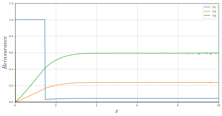
(a)

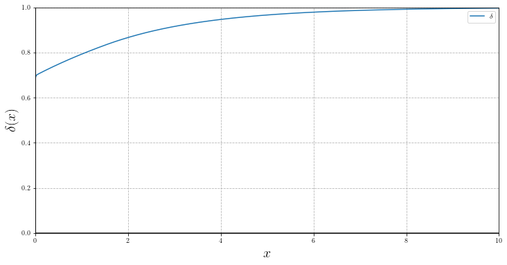
(b)

Figure 1: Three lines of insurance with three proportional reinsurance: (a) Optimal retained Proportion. (b) Survival probability function with Proportional reinsurance.

Example 4.1

Let $F_{i}(x)=1-e^{-\lambda_{i}x}$, $i=1,2,3$, and $\lambda_{1}=0.15,\,\,\lambda_{2}=0.8,\,\,\lambda_{3}=2,\,\,\beta_{1}=1,\,\,\beta_{2}=13,\,\,\beta_{3}=30,\,\,\eta=3$ and $\eta_{1}=3.5$. The reinsurance strategy in $i$th line is depicted by $R_{i}$. As was mentioned before, if $R_{i}\in\mathcal{R}_{p}$ then $R_{i}(y)=b_{i}(.)y$ and if $R_{i}\in\mathcal{R}_{XL}$ then $R_{i}(y)=\min(y,M(.))$, where $b_{i}(.)$ and $M_{i}(.)$ are functions of the company’s capital. If the insurance company considers a reinsurance contract for three lines, the optimization issue will be equal with the uni-dimensional model scrutinized by Azcue & Muler (2014). Figure 1, illustrates rules for the state in which three proportional reinsurance strategies for three lines have been used (this contract could vary from one line to another), followed by Figure 2, displaying the state in which one proportional reinsurance is used for all three lines. Furthermore, If we supplant the proportional reinsurance contract with an excess-of-loss reinsurance, the results would be as Figure 3, where 3(a), illustrates three reinsurance strategies in three insurance lines, and 3(b) and 3(c) indicate the charts for reinsurancee strategies of line 2 and 3 (which are the same). In both states, in the sense of increasing the survival function, the use of three appropriate reinsurance contracts would culminate in better results than the use of one contract for all three lines.

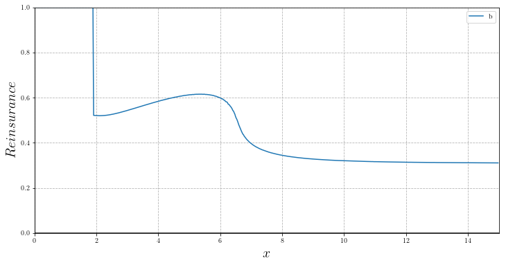
(a)

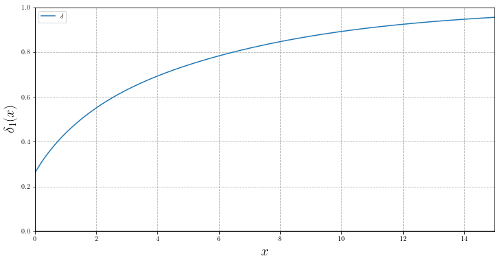
(b)

Figure 2: Three lines of insurance with one proportional reinsurance: (a) Optimal retained Proportion. (b) Survival probability function with reinsurance.

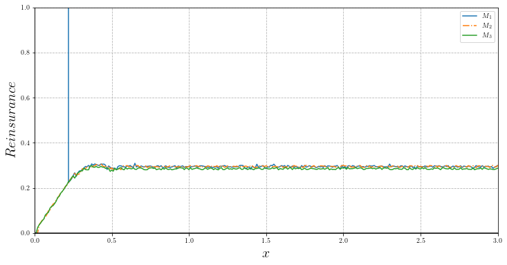
(a)

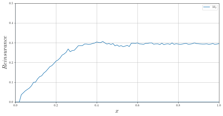
(b)

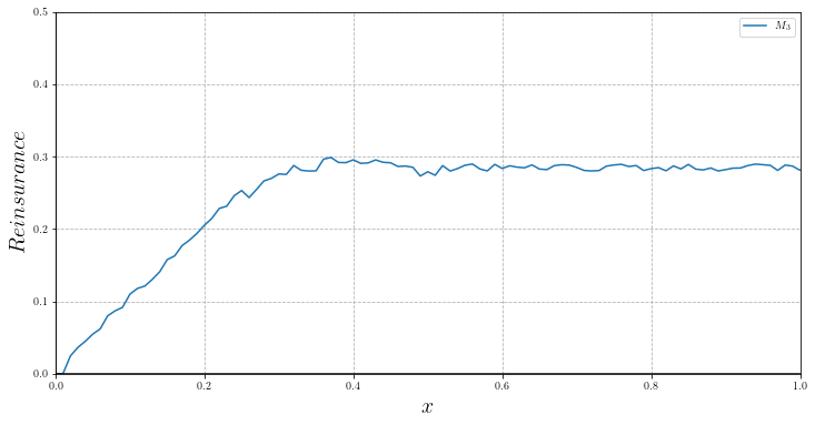
(c)

(d)

Figure 3: Three lines of insurance with three excess-of-loss reinsurance: (a) Optimal retention levels for excess-of-loss reinsurances on the first, second and third lines. (b) Optimal retention level for excess-of-loss reinsurance on second line. (c) Optimal retention level for excess-of-loss reinsurance on third line(d) Survival probability function with excess-of-loss reinsurance.

In Figure 5, the diagrams for the optimal survival function in the states of three excess-of-loss reinsurance strategies for three lines, one excess-of-loss reinsurance strategy for three lines, three proportional reinsurance strategies for three lines, one proportional reinsurance strategy for three lines and without reinsurances have been juxtaposed.

As evident from the figures (1-5), one could note that these results could be useful for the insurer such that he/she can draw different contracts. By doing this, the insurer can decrease the probability of bankruptcy vis-à-vis the state that he/she uses only one contract.

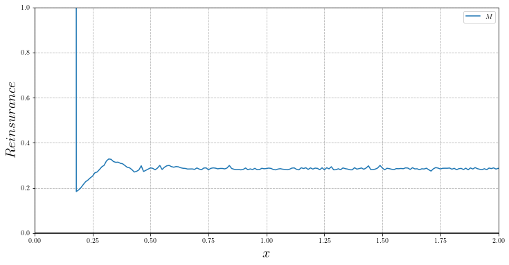
(a)

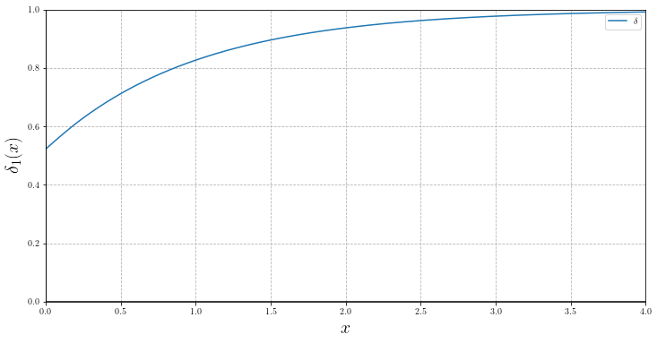
(b)

Figure 4: Three lines of insurance with one excess of loss reinsurance: (a) Optimal retention levels for excess-of-loss reinsurance (b) Survival probability function with excess-of-loss reinsurance.

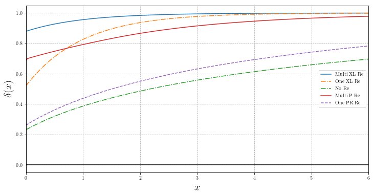
Figure 5: Survival functions

In the previous example, the exponential distribution is considered for the claims size, and only one type of reinsurance strategy is used to transfer the risk to the secondary insurer on all lines. In practice, however, the distribution of claims in each line may be completely different from the other one and the insurance company may use different types of reinsurance contracts.

Example 4.2

In this example, we consider the light-tailed distribution $F_{1}(x)=1-e^{-0.5x}$ for the claims size in the first line, the heavy-tailed distribution $F_{2}(x)=1-(\frac{3}{3+x})^{3}$ for claims size in the second line and the mixture of heavy-tailed distribution and light-tailed distribution $F_{3}(x)=0.7F_{1}(x)+0.3F_{2}(x)$ for claims size in the last line. If one of the excess-of-loss or proportional reinsurance strategies is used to control the risk of each line, then all possible settings are as follows:

• $R_{i}\in\mathcal{R}_{p},\,i=1,2,3$,

• $R_{i}\in\mathcal{R}_{p},\,i=1,2$ and $R_{3}\in\mathcal{R}_{XL}$

• $R_{i}\in\mathcal{R}_{p},\,i=1,3$ and $R_{2}\in\mathcal{R}_{XL}$

• $R_{i}\in\mathcal{R}_{p},\,i=2,3$ and $R_{1}\in\mathcal{R}_{XL}$

• $R_{i}\in\mathcal{R}_{XL},\,i=1,2$ and $R_{3}\in\mathcal{R}_{p}$

• $R_{i}\in\mathcal{R}_{XL},\,i=1,3$ and $R_{2}\in\mathcal{R}_{p}$

• $R_{i}\in\mathcal{R}_{XL},\,i=2,3$ and $R_{1}\in\mathcal{R}_{p}$

• $R_{i}\in\mathcal{R}_{XL},\,i=1,2,3$.

The optimization results for all of the above states are presented in Figure 6. As it is displayed in the Figure, in all states in which XL has been considered for the line 1, $M_{1}(x)$ is equal to zero. In Figure 7(a), for $h=0.01$ and $h=0.0004$,$M_{1}(x)$ has been presented for state $(viii)$. In effect, the smaller the $\Delta$ in the FDM, the closer the m1 to zero. Moreover, in Figure 7, the graph pertained to survival probability is reported in the all 8 above states. As it is displayed in the Figure, the best state is the one in which all lines resort to the XL reinsurance contract. As seen in Figure 7(b), if we decide to resort to the XL strategy only in one line, the best line would be line 2 in which the probability of bigger claims’ size occurring would be higher from the other two lines; furthermore, as it is observed in the Figure 7(c), if we opt for using the XL strategy in two lines, lines 2 and 3 would be efficient choices.

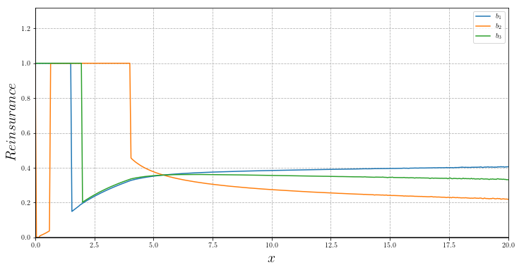
(a)

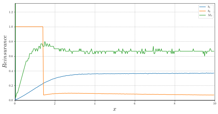
(b)

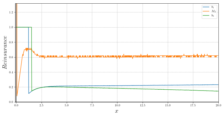
(c)

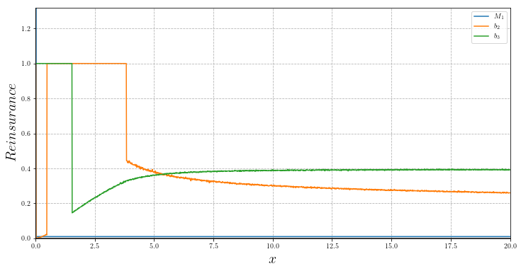
(d)

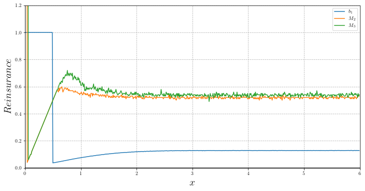
(e)

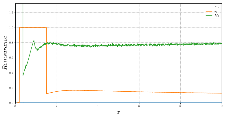
(f)

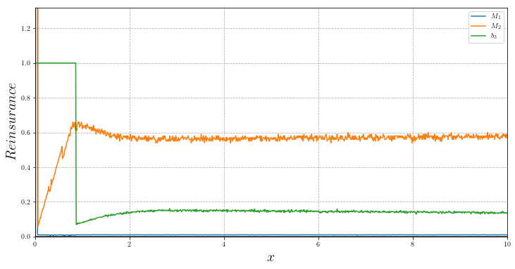
(g)

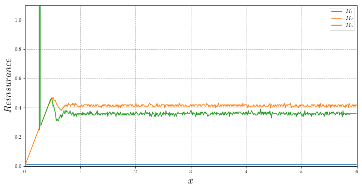
(h)

Figure 6: Optimal reinsurance strategies for states $(i)-(viii)$.

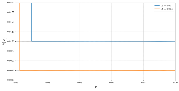
(a)

(b)

(c)

(d)

Figure 7: (a) The numerical solution of the function $M_{1}(.)$ for $h=0.01$ and $h=0.0004$ (b) Optimal survival functions for cases where only one XL contract is used (c) Optimal survival functions for cases that use two XL contracts (d) Survival functions for all possible cases

The results and findings of this paper reveal that the use of optimal dynamic reinsurance strategies increases the survival function in contrast to the use of one optimal reinsurance strategy in all lines, where a plausible question was raised on the practicality at resorting to the optimal reinsurance. Perhaps at first glance the answer could be a simple no. Indeed, for an insurance company and the reinsurer, implementing a contract which is dependent on the state of the surplus process and at any moment it may change could be extremely difficult, if not impossible. Nonetheless, it can be concluded that there is an interesting point discernible in Figures, indicating the fact that the XL strategy is a more viable option than the proportional strategy in terms of increasing the survival function. Moreover, ostensibly the XL reinsurance contracts oscillate under the circumstances that the capital of the company dwindle and the company is in the critical condition; they seem constant for increased capital. For instance, consider the previous example; if three XL reinsurances for three lines have been used, as long as the company’s assets belong to interval $(0.5,\infty)$, the reinsurance contracts are constant and they only change when the assets of the company belong to the interval $(0,0.5)$.

5 Discussion

The issue of dynamic reinsurer strategy is an interesting and efficacious approach for augmenting the survival of an insurance company and one can find a great number of studies in literature on the topic of maximizing the survival function with respect to the reinsurance strategy. In order to solve this optimization issue, an HJB equation associated with the survival function is adapted. Often, the survival function does not have the smoothness properties needed to interpret it as a solution for the corresponding HJB equation in the classical sense, but it is satisfying in this equation in a weaker concept. The present paper deals with the issue of maximization of the survival function with respect to the dynamic reinurance strategy with this difference that the insurance company shares the potential risk with several reinsurers each pertained to a specified line. The optimal survival function is characterized as the unique non-decreasing viscosity solution of (2.9) with limit one at infinity. Unfortunately, obtaining a closed form for the survival function or the reinsurance strategy in the issue discussed at this paper is fiendishly complicated or well-nigh impossible. Therefore, it was more feasible to adopt the numerical solution. For constructing a numerical solution, the FDM has been employed due to the fact that the convergence of the numerical solution to the survival function can be proved through the techniques prevalent in the literature. The convergent findings are displayed in section 4.

The results of the present paper give the insurances companies this stupendous opportunity to share their risk with the reinsurers. In section 5, there are some examples that indicate the fact that using this approach, the survival function will be increased. In a nutshell, with the implementation of this dynamic method for drawing the vector of the reinsurance contracts, the probability of bankruptcy might diminish significantly.

Appendix

Proofs of Lemma 3.1, Lemma 3.2 and Lemma 3.3 are very similar to Lemma 1.1, Proposition 2.4 and Proposition 2.12 in Azcue & Muler (2014), we therefore omit them.

Proof of Lemma 3.4. Let us prove first that $H$ is left upper semicontinuous. For assumed $x_{0}$, $x_{k}\nearrow x_{0}$, consider reinsurance strategies ${\boldsymbol{R}}^{(k)}\in\boldsymbol{\mathcal{R}}$ such that

$$\sup_{\boldsymbol{R}\in\boldsymbol{\mathcal{R}}}{\tilde{\cal{L}}}_{\boldsymbol{R}}(u)(x_{k})\leq{{\cal{L}}}_{{\boldsymbol{R}}^{(k)}}(u)(x_{k})+\frac{1}{k}.$$ (5.14)

Then, the following is straightforward,

$${{\cal{L}}}_{{\boldsymbol{R}}^{(k)}}(u)(x_{0})= {{\cal{L}}}_{{\boldsymbol{R}}^{(k)}}(u)(x_{k})+p_{{\boldsymbol{R}}^{(k)}}(u^{\prime}(x_{0})-u^{\prime}(x_{k}))-\beta(u(x_{0})-u(x_{k}))$$

$$+\int_{0}^{x_{k}}(u(x_{0}-\alpha)-u(x_{k}-\alpha))dF_{{\boldsymbol{R}}}^{(k)}(\alpha)$$

$$+\int_{x_{k}}^{x_{0}}u(x_{0}-\alpha)dF_{{\boldsymbol{R}}}^{(k)}(\alpha)$$

$$\geq {{\cal{L}}}_{{\boldsymbol{R}}^{(k)}}(u)(x_{k})+p_{{\boldsymbol{R}}^{(k)}}(u^{\prime}(x_{0})-u^{\prime}(x_{k}))-\beta(u(x_{0})-u(x_{k}))$$

$$+\int_{0}^{x_{k}}(u(x_{0}-\alpha)-u(x_{k}-\alpha))dF_{{{\boldsymbol{R}}}^{(k)}}(\alpha).$$

So, we have,

$$\limsup_{k\rightarrow\infty}{{\cal{L}}}_{{\boldsymbol{R}}^{(k)}}(u)(x_{0})\geq\limsup_{k\rightarrow\infty}{{\cal{L}}}_{{\boldsymbol{R}}^{(k)}}(u)(x_{k}).$$ (5.15)

Then, from (5.14) and (5.15), the following result can be derived;

$$\sup_{\boldsymbol{R}\in\boldsymbol{\mathcal{R}}}{{\cal{L}}}_{\boldsymbol{R}}(u)(x_{0})\geq\limsup_{k\rightarrow\infty}{{\cal{L}}}_{{\boldsymbol{R}}^{(k)}}(u)(x_{0})\geq\limsup_{k\rightarrow\infty}\left(\sup_{\boldsymbol{R}\in\boldsymbol{\mathcal{R}}}{{\cal{L}}}_{\boldsymbol{R}}(u)(x_{k})\right).$$

Consequently, the following relation is dominant $\limsup_{x\rightarrow x_{0}^{-}}\left(\sup_{\boldsymbol{R}\in\boldsymbol{\mathcal{R}}}{{\cal{L}}}_{\boldsymbol{R}}(u)(x)\right)\leq\sup_{\boldsymbol{R}\in\boldsymbol{\mathcal{R}}}{{\cal{L}}}_{\boldsymbol{R}}(u)(x_{0}).$ Now, we must prove the following $\limsup_{x\rightarrow x_{0}^{+}}\left(\sup_{\boldsymbol{R}\in\boldsymbol{\mathcal{R}}}{{\cal{L}}}_{\boldsymbol{R}}(u)(x)\right)\leq\sup_{\boldsymbol{R}\in\boldsymbol{\mathcal{R}}}{{\cal{L}}}_{\boldsymbol{R}}(u)(x_{0}).$ Given any sequence $x_{k}\searrow x_{0}$, take reinsurance strategies ${\boldsymbol{R}}^{(k)}\in\boldsymbol{\mathcal{R}}$ such that

$$\sup_{\boldsymbol{R}\in\boldsymbol{\mathcal{R}}}{{\cal{L}}}_{\boldsymbol{R}}(u)(x_{k})\leq{{\cal{L}}}_{{\boldsymbol{R}}^{(k)}}(u)(x_{k})+\frac{1}{k}.$$

If one of the reinsurance contracts is LXL reinsurance, for example $\mathcal{R}_{1}=\mathcal{R}_{LXL}$, take $\bar{{\boldsymbol{R}}}^{(k)}=(\bar{R}_{1}^{(k)},\bar{R}_{2}^{(k)},\cdots,\bar{R}_{n}^{(k)})\in\boldsymbol{\mathcal{R}}$ such that

$$\bar{R}_{1}^{(k)}(\alpha)=\begin{cases}R_{1}^{(k)}(\alpha)&if\,\,R_{1}^{(k)}(\alpha)=\alpha\,\,for\,\,all\,\,\alpha\\ R_{1}^{(k)}(\alpha)&if\,\,R_{1}^{(k)}(\alpha)=a_{k}\wedge\alpha+(\alpha-L-a_{k})^{+}\,\,with\,\,a_{k}\notin(x_{0},x_{k})\\ \alpha\wedge x_{0}+(\alpha-L-x_{0})^{+}&if\,\,R_{1}^{(k)}(\alpha)=a_{k}\wedge\alpha+(\alpha-L-a_{k})^{+}\,\,with\,\,a_{k}\in(x_{0},x_{k})\end{cases}$$

and $\bar{R}_{2}^{(k)}=R_{2}^{(k)},\cdots,\bar{R}_{n}^{(k)}=R_{n}^{(k)}$. If $a_{k}\leq x_{0}$ then

$$\int_{0}^{\infty}(u(x_{k}-\alpha)-u(x_{0}-\alpha))dF_{\bar{{\boldsymbol{R}}}^{(k)}}(\alpha)$$

$$=\int_{0}^{\infty}(u(x_{k}-\alpha)-u(x_{0}-\alpha))dF_{{\boldsymbol{R}}^{(k)}}(\alpha)$$

$$\leq\sup_{x\in[0,A]}|u^{\prime}(x)|(y-x_{0}).$$

Let us define ${{\boldsymbol{R}}}_{n-1}^{(k)}=(R_{2}^{(k)},\cdots,R_{n}^{(k)})$. If $a_{x}\in(x_{0},x_{k})$, then

$$\int_{0}^{\infty}u(x_{k}-\alpha)dF_{{{\boldsymbol{R}}}^{(k)}}(\alpha)-\int_{0}^{\infty}u(x_{0}-\alpha)dF_{\bar{{\boldsymbol{R}}}^{(k)}}(\alpha)$$

$$= \int_{0}^{\infty}\int_{0}^{\infty}u(x_{k}-R_{1}^{(k)}(\alpha_{1})-\alpha_{2})dF_{{{\boldsymbol{R}}}_{n-1}^{(k)}}(\alpha_{2})dF_{1}(\alpha_{1})-\int_{0}^{\infty}\int_{0}^{\infty}u(x_{0}-\bar{R}_{1}^{(k)}(\alpha_{1})-\alpha_{2})dF_{\bar{{\boldsymbol{R}}}_{n-1}^{(k)}}(\alpha_{2})dF_{1}(\alpha_{1})$$

$$= \int_{0}^{\infty}\int_{0}^{\infty}u(x_{k}-R_{1}^{(k)}(\alpha_{1})-\alpha_{2})dF_{{{\boldsymbol{R}}}_{n-1}^{(k)}}(\alpha_{2})dF_{1}(\alpha_{1})-\int_{0}^{\infty}\int_{0}^{\infty}u(x_{0}-\bar{R}_{1}^{(k)}(\alpha_{1})-\alpha_{2})dF_{{{\boldsymbol{R}}}_{n-1}^{(k)}}(\alpha_{2})dF_{1}(\alpha_{1})$$

$$= \int_{0}^{\infty}\int_{0}^{\infty}\big{(}u(x_{k}-R_{1}^{(k)}(\alpha_{1})-\alpha_{2})-u(x_{0}-\bar{R}_{1}^{(k)}(\alpha_{1})-\alpha_{2})dF_{{{\boldsymbol{R}}}_{n-1}^{(k)}}(\alpha_{2})\big{)}dF_{1}(\alpha_{1})$$

$$= \int_{0}^{x_{0}}\int_{0}^{\infty}\big{(}u(x_{k}-R_{1}^{(k)}(\alpha_{1})-\alpha_{2})-u(x_{0}-R_{1}^{(k)}(\alpha_{1})-\alpha_{2})dF_{{{\boldsymbol{R}}}_{n-1}^{(k)}}(\alpha_{2})\big{)}dF_{1}(\alpha_{1})$$

$$+\int_{x_{0}}^{a_{k}}\int_{0}^{\infty}\big{(}u(x_{k}-\alpha_{1}-(\alpha_{1}-L-a_{k})^{+}-\alpha_{2})-u(-(\alpha_{1}-L-x_{0})^{+}-\alpha_{2})dF_{{{\boldsymbol{R}}}_{n-1}^{(k)}}(\alpha_{2})\big{)}dF_{1}(\alpha_{1})$$

$$+\int_{a_{k}}^{x_{k}}\int_{0}^{\infty}\big{(}u(x_{k}-\alpha_{k}-(\alpha_{1}-L-a_{k})^{+}-\alpha_{2})-u(-(\alpha_{1}-L-x_{0})^{+}-\alpha_{2})dF_{{{\boldsymbol{R}}}_{n-1}^{(k)}}(\alpha_{2})\big{)}dF_{1}(\alpha_{1})$$

$$+\int_{x_{k}}^{\infty}\int_{0}^{\infty}\big{(}u(x_{k}-\alpha_{k}-(\alpha_{1}-L-a_{k})^{+}-\alpha_{2})-u(-(\alpha_{1}-L-x_{0})^{+}-\alpha_{2})dF_{{{\boldsymbol{R}}}_{n-1}^{(k)}}(\alpha_{2})\big{)}dF_{1}(\alpha_{1})$$

$$\leq\sup_{x\in[0,A]}|u^{\prime}(x)|(x_{k}-x_{0})$$

$$+\sup_{\alpha\in[x_{0},a_{k}]}(u(x_{k}-\alpha-(\alpha-L-a_{k})^{+})-u(-(\alpha-L-x_{0})^{+}))p(x_{0}\leq\alpha\leq a_{k})$$

$$+\sup_{\alpha\in[a_{k},x_{k}]}(u(x_{k}-a_{k}-(\alpha-L-a_{k})^{+})-u(-(\alpha-L-x_{0})^{+}))p(a_{k}\leq\alpha\leq x_{k})$$

$$+\sup_{\alpha\in[x_{k},\infty)}(u(x_{k}-a_{k}-(\alpha-L-a_{k})^{+})-u(-(\alpha-L-x_{0})^{+}))p(\alpha\geq x_{k})$$

According to the property of right-continuously of distribution function; if $x_{k}\searrow x_{0}$, then

$$p(x_{0}\leq\alpha\leq a_{k})\longrightarrow 0\,\,\,\,\text{and}\,\,\,\,p(a_{k}\leq\alpha\leq x_{k})\longrightarrow 0.$$

Now, the term $\sup_{\alpha\in[x_{k},\infty)}(u(x_{k}-a_{k}-(\alpha-L-a_{k})^{+})-u(-(\alpha-L-x_{0})^{+}))$ should become the focus of attention. In this case, there are two situations as outlined below:

• If, there is a finite value $m$ satisfying the following,

  $$\sup_{\alpha\in[x_{k},\infty)}(u(x_{k}-a_{k}-(\alpha-L-a_{k})^{+})-u(-(\alpha-L-x_{0})^{+}))$$

  $$=u(x_{k}-a_{k}-(m-L-a_{k})^{+})-u(-(m-L-x_{0})^{+}).$$

  So,

  $$\lim_{x_{k}\searrow x_{0}}\sup_{\alpha\in[x_{k},\infty)}(u(x_{k}-a_{k}-(\alpha-L-a_{k})^{+})-u(-(\alpha-L-x_{0})^{+}))$$

  $$=\lim_{x_{k}\searrow x_{0}}(u(x_{k}-a_{k}-(m-L-a_{k})^{+})-u(-(m-L-x_{0})^{+}))$$

  $$=u(-(m-L-x_{0})^{+})-u(-(m-L-x_{0})^{+})=0.$$

• If

  $$\sup_{\alpha\in[x_{k},\infty)}(u(xk-a_{k}-(\alpha-L-a_{k})^{+})-u(-(\alpha-L-x_{0})^{+}))$$

  $$=\lim_{\alpha\rightarrow\infty}u(x_{k}-a_{k}-(\alpha-L-a_{k})^{+})-u(-(\alpha-L-x_{0})^{+})$$

  then

  $$\sup_{\alpha\in[x_{k},\infty)}(u(xk-a_{k}-(\alpha-L-a_{k})^{+})-u(-(\alpha-L-x_{0})^{+}))=u(x_{k}-a_{k})-u(0).$$

  So,

  $$\lim_{x_{k}\searrow x_{0}}\sup_{\alpha\in[x_{k},\infty)}(u(x_{k}-a_{k}-(\alpha-L-a_{k})^{+})-u(-(\alpha-L-x_{0})^{+}))$$

  $$=\lim_{x_{k}\searrow x_{0}}(u(x_{k}-a_{k})-u(0))=0.$$

It should be noted that $R_{1}^{(k)}(\alpha)-(x_{k}-x_{0})\leq\bar{R}_{1}^{(k)}(\alpha)\leq R_{1}^{(k)}(\alpha).$ So $p_{\bar{R}_{1}^{(k)}}\nearrow p_{R_{1}^{(k)}}$. Thus

$$H(x_{k})-H(x_{0}) \leq{{\cal{L}}}_{\boldsymbol{R}^{(k)}}(u)(x_{k})-{{\cal{L}}}_{{\boldsymbol{R}}^{(k)}}(u)(x_{0})+\epsilon$$

$$\leq p_{\boldsymbol{R}^{(k)}}\sup_{x\in[0,A]}|u^{\prime\prime}(x)|(x_{k}-x_{0})+2\beta\sup_{x\in[0,A]}|u^{\prime}(x)|(x_{k}-x_{0})$$

$$+\sup_{\alpha\in[x_{0},a_{k}]}(u(x_{k}-\alpha-(\alpha-L-a_{k})^{+})-u(-(\alpha-L-x_{0})^{+}))p(x_{0}\leq\alpha\leq a_{k})$$

$$+\sup_{\alpha\in[a_{k},x_{k}]}(u(x_{k}-a_{k}-(\alpha-L-a_{k})^{+})-u(-(\alpha-L-x_{0})^{+}))p(a_{k}\leq\alpha\leq x_{k})$$

$$+\sup_{\alpha\in[x_{k},\infty)}(u(x_{k}-a_{k}-(\alpha-L-a_{k})^{+})-u(-(\alpha-L-x_{0})^{+}))p(\alpha\geq x_{k})$$

and so we get that $H$ is right upper semicontinuous. The proof for the case $\mathcal{R}_{1}=\mathcal{R}_{XL}$ and $\mathcal{R}_{1}=\mathcal{R}_{p}$ are simpler, we therefore omit them. Now, repeating the arguments presented in the proof of the Lemma 3.2 of Azcue & Muler (2014) (replacing $\boldsymbol{R}=(\boldsymbol{R}_{t})_{t\geq 0}=({R_{1}}_{t},\cdots,{R_{n}}_{t})_{t\geq 0}$ with $\bar{R}$), the following relation is obtained,

$$|H(y)-H(x_{0})|\leq K_{A}(y-x_{0}+F(y)-F(x_{0})).$$

The proof is complete. $\square$

If in Lemma 4.2 and Lemma 4.3 of Azcue & Muler (2014), replace

$${\cal{L}}_{R}(\delta)(x)=p_{R}\delta^{\prime}(x)-\beta\delta(x)+\beta\int_{0}^{x}\delta(x-\alpha)dF_{R}(\alpha)$$

with

$${\cal{L}}_{\boldsymbol{R}}(\delta)(x)=p_{\boldsymbol{R}}\delta^{\prime}(x)-(\sum_{i=1}^{n}\beta_{i})\delta(x)+(\sum_{i=1}^{n}\beta_{i})\int_{0}^{x}\delta(x-\alpha)dF_{\boldsymbol{R}}(\alpha),$$

then two lemmas Lemma 3.5 and 3.6 are derived and to prove the Lemma 3.7, it suffices to repeat the proof of Lemma 4.4 of Azcue & Muler (2014) by replacing $\boldsymbol{R}=(\boldsymbol{R}_{t})_{t\geq 0}=({R_{1}}_{t},\cdots,{R_{n}}_{t})_{t\geq 0}$ with $\bar{R}$. Therefore, proofs of these Lemmas are omitted.

proof of Lemma 3.8 (i) Assume that $i$ is a positive integer with $f^{\prime}_{h}(kh)\geq 0,k=1,...,i-1$. Then $f_{h}(0)\leq f_{h}(h)\leq\cdots\leq f_{h}((i-1)h)$ and thus

$$G_{\boldsymbol{R}}(ih)=\sum_{\{j\leq i\}}f_{h}((i-j)h)P\{(j-1)h<\boldsymbol{R}(Y)\leq jh\}\leq f_{h}((i-1)h).$$

So for $s=ih$

$$\frac{\beta f_{h}(s-h)-\beta G_{\boldsymbol{R}}(s)}{p_{{\boldsymbol{R}}}}\geq 0,$$

and thus obviously that

$$f^{\prime}_{h}(ih)=f^{\prime}_{h}(s)=\inf_{\boldsymbol{R}\in\mathcal{R}}\frac{\beta f_{h}(s-h)-\beta G_{\boldsymbol{R}}(s)}{p_{{\boldsymbol{R}}}}\geq 0,$$

which completes the induction.

(ii) The proof of this part is similar to the proof of Lemma 9 in Nozadi (2014), section 3.3. $\square$

References

- (1)
- Azcue & Muler (2014) Azcue, P. & Muler, N. (2014), Stochastic optimization in insurance: a dynamic programming approach, Springer.
- Cani & Thonhauser (2017) Cani, A. & Thonhauser, S. (2017), ‘An optimal reinsurance problem in the cramér–lundberg model’, Mathematical methods of operations research 85(2), 179–205.
- Crandall et al. (1992) Crandall, M. G., Ishii, H. & Lions, P.-L. (1992), ‘User’s guide to viscosity solutions of second order partial differential equations’, Bulletin of the American mathematical society 27(1), 1–67.
- Fleming & Soner (2006) Fleming, W. H. & Soner, H. M. (2006), Controlled Markov processes and viscosity solutions, Vol. 25, Springer Science & Business Media.
- Hipp & Taksar (2010) Hipp, C. & Taksar, M. (2010), ‘Optimal non-proportional reinsurance control’, Insurance: Mathematics and Economics 47(2), 246–254.
- Hipp & Vogt (2003) Hipp, C. & Vogt, M. (2003), ‘Optimal dynamic xl reinsurance’, ASTIN Bulletin: The Journal of the IAA 33(2), 193–207.
- Højgaard & Taksar (1998a) Højgaard, B. & Taksar, M. (1998a), ‘Optimal proportional reinsurance policies for diffusion models’, Scandinavian Actuarial Journal 1998(2), 166–180.
- Højgaard & Taksar (1998b) Højgaard, B. & Taksar, M. (1998b), ‘Optimal proportional reinsurance policies for diffusion models with transaction costs’, Insurance: Mathematics and Economics 22(1), 41–51.
- Irgens & Paulsen (2004) Irgens, C. & Paulsen, J. (2004), ‘Optimal control of risk exposure, reinsurance and investments for insurance portfolios’, Insurance: Mathematics and Economics 35(1), 21–51.
- Nozadi (2014) Nozadi, A. E. (2014), ‘Optimal constrained investment and reinsurance in lundberg insurance models’.
- Pham (2009) Pham, H. (2009), Continuous-time stochastic control and optimization with financial applications, Vol. 61, Springer Science & Business Media.
- Schmidli (2001) Schmidli, H. (2001), ‘Optimal proportional reinsurance policies in a dynamic setting’, Scandinavian Actuarial Journal 2001(1), 55–68.
- Schmidli (2004) Schmidli, H. (2004), On Cramér-Lundberg approximations for ruin probabilities under optimal excess of loss reinsurance, Laboratory of Actuarial Mathematics, University of Copenhagen.
- Schmidli (2007) Schmidli, H. (2007), Stochastic control in insurance, Springer Science & Business Media.
- Schmidli et al. (2002) Schmidli, H. et al. (2002), ‘On minimizing the ruin probability by investment and reinsurance’, The Annals of Applied Probability 12(3), 890–907.
- Taksar & Markussen (2003) Taksar, M. I. & Markussen, C. (2003), ‘Optimal dynamic reinsurance policies for large insurance portfolios’, Finance and Stochastics 7(1), 97–121.