Nonasymptotic elastoinertial turbulence for asymptotic drag reduction

Abstract

Polymer-induced drag reduction is bounded by an asymptotic limit of maximum drag reduction (MDR). For decades, researchers have presumed that MDR reflects the convergence to an ultimate flow state that is not further changed by polymers. Our simulation shows that, as drag reduction converges to its invariant limit, the underlying dynamics continues to evolve with no sign of convergence. The stage of asymptotic drag reduction is not represented by any single flow state, but encompasses states with varying dynamical patterns, all of which are partially sustained by polymer elasticity.

I Introduction

A small amount of polymer additives can cause substantial drag reduction (DR) in turbulent flows [1, 2, 3]. The effect normally increases with fluid elasticity – higher polymer concentration or molecular weight. It is, however, bounded by an asymptotic upper limit – the maximum DR (MDR), whose mean flow measurements are insensitive to changing polymer solution properties. For decades, MDR has remained the most coveted problem in this area. A full explanation must consistently address the questions of what keeps turbulence sustained at MDR (the “existence” question) and why MDR dynamics displays invariant DR (the “universality” question).

The earliest attempt was the “elastic sublayer” model by Virk [1] which considers DR effects to be confined in the turbulent buffer layer. With increasing DR, the buffer layer enlarges but its growth is eventually bounded by the flow domain size, which causes MDR. Other theories paint different pictures for polymer-turbulence interactions, but they all resort to the same postulation that MDR represents an ultimate flow state where the increasing length scale affected by polymers reaches an upper limit [4, 5, 6]. This limit depends on the flow geometry rather than polymer properties, which explains the universality of MDR. However, detailed turbulent dynamics at MDR remained largely missing in all early theories [3].

This gap is closed more recently thanks to the advancement in direct numerical simulation (DNS) and flow visualization techniques, from which two promising yet diametrical views were proposed in the past decade. The first considers this ultimate state to be a form of “hibernating” turbulence, which is inherently part of Newtonian turbulence but becomes unmasked by polymer elasticity [7, 8, 9]. During hibernation, vortices are too weak to adequately stretch polymer chains and generate large polymer stress. Therefore, hibernating turbulence is minimally impacted and cannot be further suppressed by polymers. Convergence to this Newtonian flow state perfectly explains the universality of MDR. However, the scenario has hitherto not been captured in DNS where the flow often becomes laminar at high elasticity [3].

The second believes that classical turbulence, which is fueled by fluid inertia and suppressed by polymers (referred to as inertia-driven turbulence “IDT”), is replaced by a new type of turbulence in which elasticity drives instability [10, 11, 12, 13]. This elastoinertial turbulence (EIT) is easily distinguishable from IDT as its vortex structures align in the spanwise (instead of streamwise) direction. Unlike IDT, EIT exists even in 2D [14, 15, 16]. Although 3D IDT structures can arise intermittently, it is believed that they will vanish at MDR as the flow converges to a pure 2D EIT state [14]. Since EIT is self-sustaining, the existence of MDR is easily addressed. However, its universality remains an “elephant in the room”. An instability driven partially by elasticity is expected to vary with polymer properties. Meanwhile, experiments did show invariant DR in an apparent EIT regime [11]. The elastic nature of EIT and the invariant mean flow of MDR pose a theoretical paradox [3].

All existing theories are built on the premise that the converged mean flow of MDR implies its converging underlying dynamics. For half a century, MDR research is synonymous with finding an ultimate flow state that is no longer influenced by polymers – different theories only differ in what they identify as the ultimate state. This study will challenge the underlying premise altogether. We start by showing that a pure 2D form of EIT, as most recently suggested, cannot explain MDR. The dynamics of MDR must be 3D and, more importantly, it remains nonasymptotic despite the convergence of mean flow. Interestingly, both the hibernation- and EIT-based theories are parts of a more complex dynamical picture, which is revealed for the first time here.

II Formulation

We perform DNS for channel flow under fixed pressure drop. The streamwise ($x$-) and spanwise ($z$-) directions are periodic and $y$-direction is bounded by no-slip walls. The Navier-Stokes equation is coupled with the FENE-P constitutive equation [17]

$$\frac{D\boldsymbol{v}}{Dt}=-\boldsymbol{\nabla}p+\frac{\beta}{\mathrm{Re}}\nabla^{2}\boldsymbol{v}+\frac{2\left(1-\beta\right)}{\mathrm{Re}\mathrm{Wi}}\left(\boldsymbol{\nabla}\cdot\boldsymbol{\tau}_{p}\right),$$ (1)

$$\boldsymbol{\nabla}\cdot\boldsymbol{v}=0,$$ (2)

$$\frac{\mathrm{Wi}}{2}\left(\frac{D\boldsymbol{\alpha}}{Dt}-\boldsymbol{\alpha}\cdot\boldsymbol{\nabla v}-\left(\boldsymbol{\alpha}\cdot\boldsymbol{\nabla v}\right)^{\mathrm{T}}\right)=-\frac{b}{b+5}\boldsymbol{\tau}_{p},$$ (3)

$$\boldsymbol{\tau}_{p}=\frac{b+5}{b}\left(\frac{\boldsymbol{\alpha}}{1-\frac{\mathrm{tr}(\boldsymbol{\alpha})}{b}}-\left(\frac{b}{b+2}\right)\boldsymbol{\delta}\right),$$ (4)

where $\boldsymbol{\tau}_{\text{p}}$ and $\boldsymbol{\alpha}$ are polymer stress and conformation tensors: polymer extension $\propto\sqrt{\mathrm{tr}(\alpha)}$. Velocity, length, and time are nondimensionalized by the Newtonian laminar centerline velocity $U_{\text{CL}}$, half channel height $l$, and $l/U_{\text{CL}}$, respectively. Dimensionless parameters include Reynolds number $\mathrm{Re}\equiv\rho U_{\text{CL}}l/\eta$ ($\rho$ and $\eta$ are fluid density and viscosity), Weissenberg number $\mathrm{Wi}\equiv 2\lambda U_{\text{CL}}/l$ ($\lambda$ is polymer relaxation time), viscosity ratio $\beta\equiv\eta_{\text{s}}/\eta$ ($\eta_{\text{s}}$ is solvent viscosity), and finite extensibility parameter $b\equiv\max(\mathrm{tr}(\alpha))$. Quantities in turbulent inner units [18], denoted by “+”, are scaled by the friction velocity $u_{\tau}\equiv\sqrt{\tau_{\text{w}}/\rho}$ ($\tau_{\text{w}}$ is wall shear stress) and viscous length scale $l_{\text{v}}\equiv\eta/(\rho u_{\tau})$. For instantaneous quantities denoted by “*”, instantaneous wall shear stress $\tau_{\text{w}}^{*}$ is used for inner units [7]. The standard domain size is $L_{x}^{+}\times L_{y}^{+}\times L_{z}^{+}=720\times 2\mathrm{Re}_{\tau}\times 230$ ($L_{x}^{+}\times L_{y}^{+}=720\times 2\mathrm{Re}_{\tau}$ for 2D). The friction Reynolds number $\mathrm{Re}_{\tau}\equiv\rho u_{\tau}l/\eta=84.85$ and $\beta=0.97$ are fixed; $b=5000$ unless otherwise noted.

Spatial discretization uses a hybrid method combining a TVD (total variation diminishing) finite difference scheme [19] for the $\boldsymbol{v}\cdot\boldsymbol{\nabla}\boldsymbol{\alpha}$ term and a pseudo-spectral scheme for the rest [16]. Artificial diffusion, which may tamper with EIT solutions [20, 16, 14], is not used. Numerical and temporal resolutions are comparable to recent EIT studies [10, 21, 14, 15]: $N_{x}\times N_{y}\times N_{z}=256\times 131\times 142$ and $\delta t={{0.004-0.005}}$ for 3D and $N_{x}\times N_{y}=1280\times 369$ and $\delta t=0.001$ for 2D.

The balance of turbulent kinetic energy (TKE) $\langle k\rangle_{\mathcal{V}}\equiv(1/2)\langle\boldsymbol{v}^{\prime}\cdot\boldsymbol{v}^{\prime}\rangle_{\mathcal{V}}$ is

$$\begin{split}\frac{\partial\langle k\rangle_{\mathcal{V}}}{\partial t}&=\langle\mathcal{P}^{k}\rangle_{\mathcal{V}}-\langle\epsilon_{\text{v}}^{k}\rangle_{\mathcal{V}}-\langle\epsilon_{\text{p}}^{k}\rangle_{\mathcal{V}}\\ &=-\frac{1}{2}\int_{-1}^{1}\left\langle v_{x}^{\prime}v_{y}^{\prime}\right\rangle\frac{\partial\left\langle v_{x}\right\rangle}{\partial y}dy-\frac{2\beta}{\mathrm{Re}}\left\langle\boldsymbol{\Gamma}^{\prime}:\boldsymbol{\Gamma}^{\prime}\right\rangle_{\mathcal{V}}-\frac{2(1-\beta)}{\mathrm{ReWi}}\left\langle\boldsymbol{\tau}_{\text{p}}^{\prime}:\boldsymbol{\Gamma}^{\prime}\right\rangle_{\mathcal{V}}\end{split}$$ (5)

where terms on the right-hand side are the TKE production by inertia, TKE loss by viscous dissipation, and transfer of TKE to elastic energy, respectively [22, 3]. $\boldsymbol{\Gamma}\equiv(1/2)(\boldsymbol{\nabla}\boldsymbol{v}+(\boldsymbol{\nabla}\boldsymbol{v})^{\mathrm{T}})$; $\langle\cdot\rangle$ and $\langle\cdot\rangle_{\mathcal{V}}$ denote $xz$- and volume-average, respectively; “$\prime$” indicates fluctuating components (e.g., $\boldsymbol{v}\equiv\langle\boldsymbol{v}\rangle+\boldsymbol{v}^{\prime}$). At IDT, polymers suppress turbulence for DR and thus $-\langle\epsilon_{\text{p}}^{k}\rangle_{\mathcal{V}}$ is typically negative, while positive $-\langle\epsilon_{\text{p}}^{k}\rangle_{\mathcal{V}}$ indicates net enhancement of turbulence by elasticity.

III Results

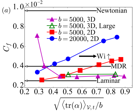
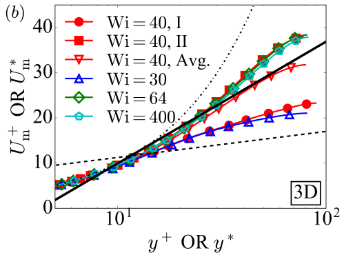
Figure 1: (a) friction factor (arrows mark Newtonian turbulence, MDR [1], and laminar values) for 2D EIT and 3D DNS (data provided in SM [23]; the “Large” domain is $2L_{x}^{+}\times L_{y}^{+}\times 2L_{z}^{+}$); (b) mean velocity profiles of 3D DNS (with reference lines: (dot-dashed) viscous sublayer $U_{\text{m}}^{+}=y^{+}$; (dashed) Newtonian log law $U_{\text{m}}^{+}=2.5\ln y^{+}+5.5$ [24]; (solid) MDR $U_{\text{m}}^{+}=11.7\ln y^{+}-17.0$ [1]; instants I and II are marked in fig. 2 and fig. 4(a)). Error bars use block average [25].

We start with 2D DNS where IDT is precluded and only EIT can exist. At $b=5000$, 2D EIT is found for $\mathrm{Wi}$ down to $40$ (fig. 1(a); also see data in the Supplemental Material (SM) [23]), where polymers are stretched, on average, to $\approx 30\%$ of full extension ($\sqrt{\langle\mathrm{tr}(\alpha)\rangle_{\mathcal{V},t}/b}\approx 0.3$; $\langle\cdot\rangle_{\mathcal{V},t}$ denotes volume and time average). Its drag, measured by the Fanning friction factor $C_{\text{f}}\equiv 2\tau_{\text{w}}/(\rho\langle v_{x}\rangle_{\mathcal{V},t}^{2})$, is barely above the laminar level. Both polymer extension and $C_{\text{f}}$ increase with $\mathrm{Wi}$. There is no apparent tendency for $C_{\text{f}}$ to converge even at the highest $\mathrm{Wi}=800$ where polymers are nearly 90% stretched. At $b=20000$, the whole $C_{\text{f}}$ curve is higher, which again rises monotonically with $\mathrm{Wi}$ without convergence. Ever growing drag enhancement (DE) with $\mathrm{Wi}$ and $b$ in elastic or elastoinertial instabilities should come as no surprise, which is common in other flow types [26]. It however reveals that, contrary to prior belief, MDR, whose $C_{\text{f}}$ is invariant with polymer parameters (including $\mathrm{Wi}$ and $b$), cannot be this 2D EIT state.

By contrast, in 3D flow, DR initially increases ($C_{\text{f}}$ decreases) with $\mathrm{Wi}$ but later converges. The last 5 data points in fig. 1(a), corresponding to $\mathrm{Wi}=64$ to $800$ (see SM [23]), show nearly the same $C_{\text{f}}$ magnitude. Mean velocity profiles (fig. 1(b)) in this range are also inseparable. The converged DR level slightly exceeds the Virk [1] MDR asymptote, which is commonly seen in DNS of comparable regimes [21, 27]. Domain size is one reason. Two cases ($\mathrm{Wi}=80$ and $400$) tested in a larger domain with doubled $x$- and $z$-dimensions (fig. 1(a)) again have nearly identical $C_{\text{f}}$. The plateau $C_{\text{f}}$ level is slightly higher than that of the standard domain, which is expected given the spatial intermittency and correlation over longer length scales. We thus expect the mean flow to better match the Virk asymptote in larger domains. Meanwhile, the empirical MDR asymptote by Virk [1] itself contains uncertainty [28, 29], which also may not be accurate for lower $\mathrm{Re}$.

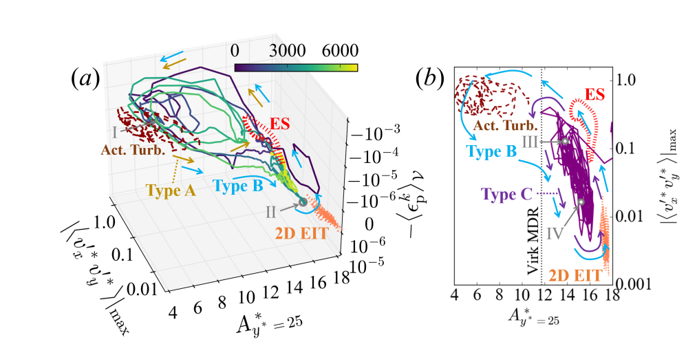
Figure 2: Dynamical trajectories of 3D DNS at (a) $\mathrm{Wi}=40$ (solid; color maps to time) and (b) $\mathrm{Wi}=400$ (solid; purple). The edge state [30] and 2D EIT solutions are both at $\mathrm{Wi}=40$; active turbulence is represented by 3D DNS solution at $\mathrm{Wi}=30$. $A^{*}\equiv y^{*}(\partial U_{\text{m}}^{*}/\partial y^{*})$ is the logarithmic slope function and $A^{*}_{y^{*}=25}$ measures the local steepness of the $U^{*}_{\text{m}}(y^{*})$ profile at $y^{*}=25$ [3]. $|\langle v_{x}^{\prime*}v_{y}^{\prime*}\rangle|_{\text{max}}$ is the maximum instantaneous Reynolds shear stress value (after $xz$-average) [30, 22].

The underlying dynamics undergoes transitions between 3 types of cycles. The $\mathrm{Wi}=40$ trajectory (fig. 2(a)), which is right before the asymptotic convergence of $C_{\text{f}}$, shows type A and type B cycles. Both types take the state away from active turbulence – the dominant form of turbulence of Newtonian flow and lower $\mathrm{Wi}$ characterized by lower mean velocity and higher Reynolds stresses [7, 8, 3]. Type A cycles visit the vicinity of the edge state (ES) – an invariant solution that separates laminarizing trajectories from those staying turbulent [31, 30]. These visits are known to be hibernating turbulence [30, 32]. Intermittent active-hibernating cycles occur in IDT even in Newtonian flow and their statistical weight increases with $\mathrm{Wi}$ [7, 8, 22, 33]. During type B cycles, which are not seen at lower $\mathrm{Wi}$ and reported for the first time here, the flow approaches EIT first and then pivots and returns via the ES region. At the high $\mathrm{Wi}$ limit, represented by $\mathrm{Wi}=400$ in fig. 2(b), the dynamics collapses to a new type C cycle (also never reported before) which appears to bounce back and forth between the vicinities of ES and 2D EIT and strong active turbulence is never triggered.

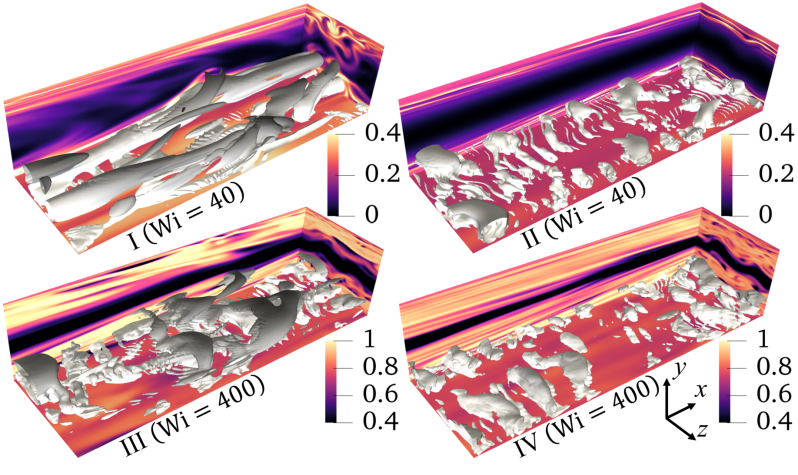
Figure 3: Flow structures of 3D DNS at representative instants as marked in figs. 2, 4 and 5. Colors map to $\mathrm{tr}(\alpha)/b$. Isosurfaces show vortex configuration using the $Q$-criterion [34, 35] ($Q=0.004$; bottom half channel only).

Figure 3 shows flow structures of different dynamical phases. Active turbulence (instant I) shows classical streamwise vortices (some spanwise structures spotted near the wall are likely residues of EIT). Its instantaneous $U_{\text{m}}^{*}(y^{*})$ profile (fig. 1(b)) reflects features of drag-reduced IDT and resembles the time-average profiles of lower $\mathrm{Wi}$. Instant II represents the EIT region visited during type B cycles and features trains of spanwise vortex rolls spaced by thinner threads. Despite capturing key features of 2D EIT [14, 15, 16], it is not strictly 2D. Indeed, 3D DNS never fully reaches 2D EIT (fig. 2), especially at higher $\mathrm{Wi}$ where 2D EIT has much higher $C_{\text{f}}$ (fig. 1(a)). Instantaneous velocity of II (fig. 1(b)) matches the asymptotic DR level of $\mathrm{Wi}=$ $64800$ even though at $\mathrm{Wi}=40$ the time average profile is still lower. Instants III and IV represent two different phases of type C cycles. Although IV appears similar to II (and thus to 2D EIT), III shows distinct hairpin-like structures in addition to spanwise vortices. They are probably unrelated with hairpin vortices in Newtonian flow typically observed at higher $\mathrm{Re}$ [36, 37, 35] and possibly result from a fusion between spanwise rolls of EIT and streamwise vortices of IDT (including the ES).

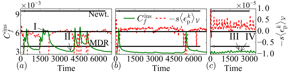
Figure 4: Time series of instantaneous friction factor $C_{\text{f}}^{\text{ins}}$ and TKE elastic conversion rate $-\langle\epsilon_{\text{p}}^{k}\rangle_{\mathcal{V}}$ (scaled by a factor $s$ for clarity) of 3D DNS: (a) $\mathrm{Wi}=40$ ($s=20$) showing types A and B cycles, (b) $\mathrm{Wi}=64$ ($s=12$) showing type B cycles, and (c) $\mathrm{Wi}=400$ ($s=4$) showing type C cycles. Arrows mark $C_{\text{f}}$ of Newtonian turbulence and MDR.

Instantaneous friction factor $C_{\text{f}}^{\text{ins}}\equiv 2\tau_{\text{w}}^{*}(t)/(\rho\langle v_{x}\rangle_{\mathcal{V}}^{2})$ at $\mathrm{Wi=40}$ (fig. 4(a)) shows intermittent dives separated by spikes. The spikes reflect returns to active turbulence, which is accompanied by strong negative $-\langle\epsilon_{\text{p}}^{k}\rangle_{\mathcal{V}}$ showing that stretched polymers suppress turbulence. Type A cycles display shallow dives (e.g., near $t=4500$) lasting for $O(100)$ time units (TUs). These hibernating intervals still belong to IDT with negative $-\langle\epsilon_{\text{p}}^{k}\rangle_{\mathcal{V}}$ but their $C_{\text{f}}^{\text{ins}}$ can approach the MDR level. Type B cycles show deeper dives lasting for $O(1000)$ TUs with lower $C_{\text{f}}^{\text{ins}}$. They spend most time near EIT where $-\langle\epsilon_{\text{p}}^{k}\rangle_{\mathcal{V}}$ turns positive.

The hibernation-based theory conjectures that, with increasing $\mathrm{Wi}$, active turbulence diminishes and the flow converges to the ultimate state of hibernation [7, 8], because the ES would persist as an invariant barrier that blocks it from laminarization [31, 30]. Findings here show that at higher $\mathrm{Wi}$, the flow can move past the ES and EIT steps up as the second line of defense to keep turbulence sustained. The $\mathrm{Wi}=40$ case, where $C_{\text{f}}$ has not yet converged, is in the middle of this transition. At $\mathrm{Wi}=64$, where $C_{\text{f}}$ starts to plateau, type A cycles disappear (fig. 4(b)) and EIT becomes solely responsible for pivoting laminarizing trajectories. The dives are also significantly prolonged. If $\mathrm{Re}$ were lower, bypass of the ES could occur before EIT emerges. There would then be a window of $\mathrm{Wi}$ where the flow laminarizes, as observed in recent experiments [11, 13].

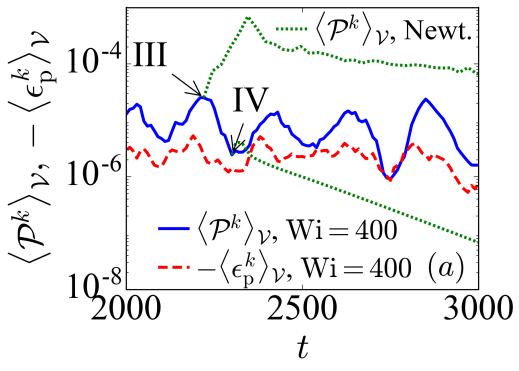
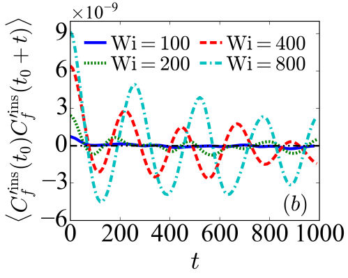
Figure 5: (a): enlargement of type C cycle (fig. 4(c)) time series, with Newtonian shooting trajectories showing the dynamics after removing polymer stress from instants III and IV; (b) time autocorrelation function of $C_{\text{f}}^{\prime,\text{ins}}$ (3D DNS).

Strikingly, despite $C_{\text{f}}$ converging from $\mathrm{Wi}=64$ up to $\mathrm{Wi}=800$ tested (fig. 1(a)), dynamical patterns change again for $\mathrm{Wi}\gtrsim 200$. At $\mathrm{Wi}=400$ shown in fig. 4(c), intermittent $C_{\text{f}}^{\text{ins}}$ spikes are replaced by smaller quasi-periodic wiggles. These type C cycles also show much higher frequency than both previous types. Each cycle (fig. 5(a)) starts with the rise of $-\langle\epsilon_{\text{p}}^{k}\rangle_{\mathcal{V}}$, which quickly sparks a stronger inertial instability, marked by a much higher peak in TKE production $\langle\mathcal{P}^{k}\rangle_{\mathcal{V}}$. The net $-\langle\epsilon_{\text{p}}^{k}\rangle_{\mathcal{V}}$ remains non-negative, because even at highest $\langle\mathcal{P}^{k}\rangle_{\mathcal{V}}$ (instant III) substantial EIT structures persist especially near the wall (fig. 3) and $-\langle\epsilon_{\text{p}}^{k}\rangle_{\mathcal{V}}$ is a spatial average of both IDT (negative $-\langle\epsilon_{\text{p}}^{k}\rangle_{\mathcal{V}}$) and EIT (positive $-\langle\epsilon_{\text{p}}^{k}\rangle_{\mathcal{V}}$) structures. Nonetheless, if we remove polymer stress at instant III (i.e., Newtonian DNS using its flow field as the initial state), full scale IDT will develop (fig. 5(a)). By contrast, during the quiescent phase (instant IV), removing polymer stress would instead cause laminarization. EIT is thus required to trigger the next cycle and sustain turbulence.

Figure 5(b) shows the time autocorrelation function of the fluctuating component of $C_{\text{f}}^{\text{ins}}$. At $\mathrm{Wi}=100$, the dynamics remains chaotic and the correlation decays monotonically. Oscillatory patterns appear at $\mathrm{Wi}=200$ as the first sign of quasi-periodicity. The dynamics continues to evolve afterwards. The amplitude of oscillation increases with $\mathrm{Wi}$ up to the highest level of $800$ tested while its frequency decreases.

IV Conclusions

In summary, we find that for a wide range of $\mathrm{Wi}$ ($64$ to $800$) where DR has reached its asymptotic level, the underlying dynamics never converges. Intermittent dynamics involving bursts of active turbulence persists up to $\mathrm{Wi}\approx 200$, after which quasi-periodic oscillation dominates. The pattern of oscillation continues to evolve with $\mathrm{Wi}$. As such, the long-standing premise of MDR being a converged ultimate state must be reexamined and continued search of such a single flow state would be misguided.

The earlier hibernation-based theory describes the dynamics accurately up to a moderate $\mathrm{Wi}$ level, but direct hibernation is later bypassed, exposing EIT as the second barrier before laminarization. The EIT-based theory also appears over-simplistic. The flow does not converge to a pure 2D form of EIT. The phenomenological MDR encompasses an ensemble of different self-sustaining turbulent processes which all share the same mean drag. One may, of course, generalize the concept of EIT to cover all types of turbulence where elasticity is essential for sustained instability, so that all different states within MDR fall under this umbrella. However, that would not erase the nonasymptotic nature of MDR (at least in the low-$\mathrm{Re}$ regime studied), which has never been revealed before.

In a larger simulation domain, both intermittent ($\mathrm{Wi}=80$) and quasi-periodic ($\mathrm{Wi}=400$) dynamics are again observed while $C_{\text{f}}$ stays invariant. In those solutions, characteristic structures of different dynamical phases, e.g., active turbulence and EIT, are seen to coexist in different regions of the domain, suggesting that temporal intermittency observed in small domains would map to spatial intermittency in experimental flow scales.