A new self-consistent approach of quantum turbulence in superfluid helium

Abstract

We present the Fully cOUpled loCAl model of sUperfLuid Turbulence (FOUCAULT) that describes the dynamics of finite temperature superfluids. The superfluid component is described by the vortex filament method while the normal fluid is governed by a modified Navier-Stokes equation. The superfluid vortex lines and normal fluid components are fully coupled in a self-consistent manner by the friction force, which induce local disturbances in the normal fluid in the vicinity of vortex lines. The main focus of this work is the numerical scheme for distributing the friction force to the mesh points where the normal fluid is defined and for evaluating the velocity of the normal fluid on the Lagrangian discretization points along the vortex lines. In particular, we show that if this numerical scheme is not careful enough, spurious results may occur. The new scheme which we propose to overcome these difficulties is based on physical principles. Finally, we apply the new method to the problem of the motion of a superfluid vortex ring in a stationary normal fluid and in a turbulent normal fluid.

I Introduction

Quantum turbulence vinen-niemela-2002 ; skrbek-sreenivasan-2012 ; barenghi-skrbek-sreenivasan-2014 is the disordered motion of quantum fluids - fluids which are governed by the laws of quantum mechanics rather than classical physics. Examples of quantum fluids are atomic Bose-Einstein condensates pitaevskii-stringari-2003 ; primer2016 , the low temperature liquid phases of helium isotopes ³He and ⁴He, polariton condensates, and the interior of neutron stars. The underlying physics is the condensation of atoms which obey Bose-Einstein statistics. In this work we focus on the superfluid phase of ⁴He, frequently referred to as helium-II or He-II for short. Helium II can be described as an intimate mixture of two fluid components tisza-1938 ; landau-1941 : the viscous normal fluid, which is similar to ordinary viscous fluids obeying the classical Navier-Stokes equation, and the inviscid superfluid, whose vorticity is confined to vortex lines of atomic thickness and quantised circulation (also referred to as quantised vortices or superfluid vortices). At nonzero temperatures, quantum turbulence thus manifests itself as a disordered tangle of vortex lines interacting with either a laminar or a turbulent normal fluid depending on the circumstances.

Despite the two-fluid nature and the quantisation of superfluid vorticity, several surprising analogies between classical turbulence and quantum turbulence have been established in helium II in the last years. One example is the same temporal decay of vorticity stalp-skrbek-donnelly-1999 in unforced turbulence. Another example is the energy spectrum of forced homogeneous isotropic turbulence, which, according to experiments maurer-tabeling-1998 ; salort-etal-2010 ; barenghi-lvov-roche-2014 , numerical simulations baggaley-laurie-barenghi-2012 ; baggaley-barenghi-2011 ; araki-tsubota-nemirovskii-2002 ; kobayashi-tsubota-2005 and theory lvov-nazarenko-skrbek-2006 ; lvov-nazarenko-rudenko-2008 , displays the same Kolmogorov energy spectrum (the distribution of kinetic energy over the length scales) which is observed in classical turbulence. However, at sufficiently small length scales (smaller than the average inter-vortex distance), or when superfluid and normal fluid are driven thermally in opposite directions vinen-1957a ; barenghi-sergeev-baggaley-2017 , fundamental differences emerge between classical and quantum turbulence lamantia-duda-rotter-skrbek-2013b ; lamantia-2017 .

The comparison between quantum and classical turbulence is therefore a current topic of lively discussions in low temperature physics community. Essential progress in the understanding of the underlying physics is provided by the recent development of new experimental techniques for the visualisation of superfluid helium flows, including micron-sized tracers, polymer particles zhang-vansciver-2005 , solid hydrogen/deuterium flakes bewley-lathrop-sreenivasan-2006 ; lamantia-chagovets-rotter-skrbek-2012 and, more recently, smaller (thus less intrusive) metastable helium molecules guo-etal-2010 which fluoresce when excited by a laser.

Alongside experiments, numerical simulations have played an important role in understanding the physics of quantum turbulence, from interpreting experimental data to proposing new experiments. However, most numerical simulations have determined the motion of vortex lines as a function of prescribed normal fluid profiles without taking into account the back-reaction of the vortex lines hanninen-baggaley-2014 onto the normal fluid. Only a small number of investigations have addressed this back-reaction, but most efforts have suffered from some shortcomings: they were restricted to two-dimensional channels galantucci-sciacca-barenghi-2015 ; galantucci-sciacca-barenghi-2017 , had too limited numerical resolution to address fully developed turbulence yui-etal-2018 , considered only simple vortex configurations kivotides-barenghi-samuels-2000 ; idowu-willis-barenghi-samuels-2000 , were limited to decaying turbulence kivotides-2015jltp ), or did not reach the statistically steady-state which is necessary to make direct comparison to classical turbulence.

This work presents a fully-coupled, three dimensional numerical model which tackles all these shortcomings and contains innovative features concerning the numerical architecture and the physical modelling of the interaction between normal fluid and vortex lines. We shall refer to our model as FOUCAULT, Fully-cOUpled loCAl model of sUperfLuid Turbulence. Compared to past studies, our model consists of an efficiently parallelised pseudo-spectral code capable of distributing the calculation of the normal fluid velocity field and the temporal evolution of the superfluid vortex tangle amongst distinct computational cluster nodes. This feature allows the resolution of a wider range of flow length scales compared to the previous literature, spanning large quasi-classical length scales as well as smaller quantum length scales. This wide range is of fundamental importance for the numerical simulation of turbulent flows of helium II with realistic experimental parameters.

From the physical point of view, FOUCAULT includes a new approach to determine the friction force between superfluid vortices and the normal fluid, developed from progress in the study of classical creeping flows kivotides-2018 , but modified in order to avoid the unphysical dependence of the friction on the numerical discretization on the vortex lines. In addition, the force between the vortices and the normal fluid (ideally a Dirac delta function centred on the vortex lines) is regularised exactly employing a method recently developed in classical turbulence gualtieri_picano_sardina_casciola_2015 ; GualtieriPREActiveParticlesPRE for the consistent modelling of the two-way coupling between a viscous fluid and small active particles. This method stems from the small-scale viscous diffusion of the normal fluid disturbances generated by the vortex motion, thus regularising the fluid response to vortex forcing in a physically consistent manner. Our fully-coupled local model is therefore a significant improvement with respect to previous algorithms which employed arbitrary numerical procedures for the distribution of the vortex forcing on the Eulerian computational grid of the normal fluid kivotides-2011 .

The organisation of the paper is the following. In Section II we describe the equations of motion of the superfluid, the normal fluid and the vortex lines with emphasis on the different existing models for the calculation of the friction force. In Section III we outline our numerical method, including details on the Vortex Filament Method, the Navier–Stokes solver, interpolation schemes and the procedure employed for regularising the friction force consistently. Next, in Section IV, we show two applications of our model. Finally, in Section V we summarise the main points and outline future work.

II Equations of Motions

II.1 Helium II

If the temperature of liquid helium is lowered below $T_{\lambda}=2.17~{}\rm K$ at saturated vapour pressure, a second order phase transition takes place to another liquid phase, known as helium II, which exhibits quantum-mechanical effects (unlike the high-temperature phase above $T_{\lambda}$, called helium I, which can be adequately described as an ordinary Newtonian fluid). In the absence of vortex lines, the motion of helium II is well described by the two-fluid model of Landau and Tisza. This model describes helium II as the intimate mixture of two co-penetrating fluid components tisza-1938 ; landau-1941 ; london-1954 ; donnelly-1991 ; nemirovskii-2013 , which can be accelerated by temperature and/or pressure gradients: the viscous normal fluid and the inviscid superfluid. Each component is characterised by its own kinematic and thermodynamic fluid variables. In this description, the total density of helium II, $\rho$, is the sum of the partial densities $\rho_{n}$ and $\rho_{s}$ of the normal fluid and the superfluid: $\rho=\rho_{n}+\rho_{s}$ (hereafter we use the subscripts ’$n$’ and ’$s$’ to refer to normal fluid and superfluid components, respectively). While $\rho$ is approximately independent of temperature for $T<T_{\lambda}$, the superfluid and normal fluid densities are strongly temperature dependent: in the limit $T\to T_{\lambda}$, helium II becomes entirely normal ($\rho_{n}/\rho\to 1$), whereas in the limit $T\to 0$ it becomes entirely superfluid ($\rho_{s}/\rho\to 1$). In practice, as the normal fluid density decreases quite rapidly with decreasing temperature, a helium sample at $T\leq 1~{}\rm K$ is effectively a pure superfluid ($\rho_{s}/\rho\geq 0.99$).

Loosely speaking, the superfluid component corresponds to the quantum ground state of the system governed by a macroscopic complex wavefunction $\Psi$, and the normal fluid corresponds to thermal excitations (strictly speaking, this identification of the superfluid component with the condensate is not correct: helium II is a liquid of interacting bosons, not a weakly interacting gas). At temperatures of the most experimental interest, the mean free path of the thermal excitations is short enough that the normal fluid behaves like an ordinary (classical) viscous fluid with non-vanishing dynamic viscosity and entropy per unit mass, $\eta$ and $s$ respectively. In contrast, the superfluid component is inviscid and incapable of carrying entropy (hence heat). Physically, the existence of two distinct velocity fields $\mathbf{v}_{n}$ and $\mathbf{v}_{s}$ signifies that, locally, two simultaneous distinct movements are possible, even though individual helium atoms cannot be separated into two components.

However, if helium II rotates, or if the relative speed $v_{ns}=|\mathbf{v}_{n}-\mathbf{v}_{s}|$ between normal fluid and superfluid exceeds a critical value, superfluid vortex lines nucleate, coupling the two fluids donnelly-1991 ; nemirovskii-2013 in a way that invalidates the model of Landau and Tisza. It is instructive to write the superfluid wavefunction $\Psi$ in terms of its amplitude and phase, $\Psi=|\Psi|e^{i\phi}$, and use the quantum mechanical prescription relating the velocity to the gradient of the phase: $\mathbf{v}_{s}=(\hbar/m)\nabla\phi$. One finds primer2016 that a vortex line is a topological defect: a one-dimensional region in three-dimensional space where the phase $\phi$ is undefined, and the magnitude $|\Psi|$ vanishes exactly. Vortex lines are thus nodal lines of the wavfunction. The single valuedness of the wavefunction implies that the circulation integral $\Gamma$ following a closed path $C$ is either zero (if $C$ does not encircle the vortex line), or takes the fixed value

$$\Gamma=\oint_{C}\mathbf{v}_{s}\cdot d\mathbf{l}=\kappa,$$ (1)

if $C$ encircles the vortex line, where $\kappa=h/m$ is the quantum of circulation. A multiply-charged vortex line carrying more than one quantum of circulation is usually unstable, breaking into many singly-charged vortex lines. Eq. (1) also implies that the superfluid velocity around a straight vortex line has the form $v_{s}=\kappa/(2\pi r)$, where $r$ is the distance to the vortex axis. Since the superfluid component has zero viscosity, this azimuthal velocity field persists forever. Notice that the corresponding superfluid vorticity is a Dirac delta function defined on the vortex axis.

Physically, we can think of a vortex line as a thin tubular hole (centred on the vortex axis) around which the circulation has the fixed value $\kappa$. The radius of the hole is also fixed by quantum mechanics, and has the value $a_{0}\approx 10^{-10}\rm m$, which is the characteristic distance over which the amplitude of $\Psi$ drops from its bulk value (at infinity, away from the vortex) to zero (on the vortex axis).

Vortex lines act as scattering centers for the thermal excitations (phonons and rotons) constituting the normal fluid hall-vinen-1956a ; hall-vinen-1956b . This interaction produces an exchange of momentum, hence a mutual friction force $\mathbf{F}_{ns}$, between the superfluid component and the normal fluid component. The quantisation of the superfluid circulation and the friction force between superfluid and normal fluid make helium II a more complex, richer system than the original two-fluid scenario of Landau and Tisza.

This aim of this work is to develop a suitable numerical framework to address simultaneously the coupled temporal evolution of (i) the normal fluid velocity field and (ii) the superfluid vortex lines, taking the friction into account. In the following Sections II.2 - II.5 we outline the equations of motions of the fluid components, the superfluid vortex lines and the expression of the friction force employed in our numerical algorithm.

II.2 The normal fluid

The normal fluid is a gas of elementary excitations called phonons and rotons. In the range of temperatures which we are interested in, namely ${1.5\rm~{}K}<T<T_{\lambda}$, the normal fluid density is mostly due to rotons hall-vinen-1956b . The roton mean free path is bdv1982 $\lambda_{mfp}=3\eta/(\rho_{n}v_{G})$, where $v_{G}=\sqrt{2k_{B}T/(\pi\mu)}$ is the roton group velocity, $\mu=0.16m_{4}$ is the roton effective mass brooks-donnelly-1977 and $m_{4}=6.65\times 10^{-27}\rm kg$ is the helium mass; therefore $\lambda_{mfp}$ varies from $13\times 10^{-10}\rm m$ at $T=1.5\rm K$ to $2.2\times 10^{-10}\rm m$ at $T=2.15~{}\rm K$. These values are much smaller than the typical intervortex distance, $\ell\approx 10^{-6}\rm m$ to $10^{-4}\rm m$, at the flow’s small scales, and the current experimental facilities at the flow’s large scales, which typically range from $10^{-3}\rm~{}m$ to $10^{0}\rm~{}m$ svancara-lamantia-2019 ; mastracci-etal-2019 . The normal component can hence be effectively described as a fluid with its own velocity $\mathbf{v}_{n}$, density $\rho_{n}$, entropy per unit mass $s$ and dynamic viscosity $\eta$. Given the small temperature gradients observed in experiments childers-tough-1976 , $\rho_{n}$, $s$ and $\eta$ can be treated as uniform and constant properties of the fluid. Furthermore, the normal fluid can be adequately treated as a Newtonian fluid, i.e. the viscous stress tensor is linear in velocity gradients. Stemming from these physical characteristics of the normal component, a long series of studies have focused on the derivation of the equations of motion of helium II in the presence of vortex lines, at length scales $\Delta$ much larger than the average inter-vortex spacing $\ell$ hall-vinen-1956b ; bekarevich-khalatnikov-1961 ; hills-roberts-1977 : these equations of motion are nowadays referred to as the Hall-Vinen-Bekarevich-Khalatnikov (HVBK) equations. In the cited circumstance where the normal fluid undergoes incompressible isoentropic motion with constant and uniform dynamic viscosity, the HVBK equations of motion for the normal component in presence of vortex lines coincide with the Navier–Stokes equations for a classical incompressible viscous fluid with the addition of an extra term $\mathbf{F}_{ns}$ representing the friction force:

$$\displaystyle\rho_{n}\left[\frac{\partial\mathbf{v}_{n}}{\partial t}+\left(\mathbf{v}_{n}\cdot\nabla\right)\mathbf{v}_{n}\right] = -\frac{\rho_{n}}{\rho}\nabla p-\rho_{s}s\nabla T+\eta\nabla^{2}\mathbf{v}_{n}+\mathbf{F}_{ns}\;\;,$$ (2)

$$\nabla\cdot\mathbf{v}_{n} = 0\;\;,$$ (3)

where $p$ is pressure. Considering hereafter only isothermal helium II and introducing characteristic units of length and time, respectively $\lambda$ and $\tau$, Eqs. (2) and (3) can be made non-dimensional as follows:

$$\displaystyle\frac{\partial\widetilde{\mathbf{v}}_{n}}{\partial\widetilde{t}}+\left(\widetilde{\mathbf{v}}_{n}\cdot\widetilde{\nabla}\right)\widetilde{\mathbf{v}}_{n} = -\widetilde{\nabla}\widetilde{\left(\frac{p}{\rho}\right)}+\frac{\nu_{n}}{(\lambda^{2}/\tau)}\widetilde{\nabla}^{2}\widetilde{\mathbf{v}}_{n}+\left(\frac{\mathbf{F}_{ns}}{\rho_{n}}\right)\frac{\tau^{2}}{\lambda}\;\;,$$ (4)

$$\widetilde{\nabla}\cdot\widetilde{\mathbf{v}}_{n} = 0\;\;,$$ (5)

where $\widetilde{\cdot}$ indicates non-dimensional quantities and $\nu_{n}=\eta/\rho_{n}$ is the kinematic viscosity of the normal fluid. The numerical schemes for the integration of Eqs. (4) and (5) and the numerical handling of the friction force $\mathbf{F}_{ns}$ are discussed in Sections III.2 and III.4, respectively.

II.3 The superfluid

The complete set of HVBK equations consists of Eqs. (2) and (3) supplemented with the equations of motion of the superfluid component which, in the incompressible approximation and neglecting the tension force, are as follows:

$$\displaystyle\rho_{s}\left[\frac{\partial\mathbf{v}_{s}}{\partial t}+\left(\mathbf{v}_{s}\cdot\nabla\right)\mathbf{v}_{s}\right] = -\frac{\rho_{s}}{\rho}\nabla p+\rho_{s}s\nabla T-\mathbf{F}_{ns}\;\;,$$ (6)

$$\nabla\cdot\mathbf{v}_{s} = 0\;\;.$$ (7)

As already said, the superfluid vorticity $\bm{\omega}_{s}=\nabla\times\mathbf{v}_{s}$ is confined to the vortex-lines which can effectively be described as one-dimensional objects because the vortex core size $a_{0}\approx 10^{-10}\rm~{}m$ is several orders of magnitude smaller than the flow length scales probed in the present work ($\approx 10^{-5}\rm~{}m$ to $10^{-6}\rm~{}m$). The vortex lines can hence be treated as parametrised space curves $\mathbf{s}(\xi,t)$ in a three-dimensional domain, where $\xi$ is arc-length and $t$ is time. Within this mathematical description of vortex lines, the superfluid vorticity $\bm{\omega}_{s}$ can be expressed in terms of $\delta$-distributions, as follows

$$\bm{\omega}_{s}(\mathbf{x},t)=\kappa\oint_{\mathcal{L}}\mathbf{s}^{\prime}(\xi,t)\delta(\mathbf{x}-\mathbf{s}(\xi,t))d\xi\;\;\;\;,$$ (8)

where

$$\mathbf{s}^{\prime}(\xi,t)=\frac{\partial\mathbf{s}(\xi,t)}{\partial\xi},$$ (9)

is the unit tangent vector to the curve $\mathbf{s}(\xi,t)$ and $\mathcal{L}$ indicates the whole vortex configuration.

The superfluid velocity may hence be expressed in terms of the spatial distribution of vortex lines $\mathbf{s}(\xi,t)$ via the Biot-Savart integral schwarz-1978 , i.e.

$$\mathbf{v}_{s}(\mathbf{x},t)=\nabla\phi(\mathbf{x},t)+\frac{\kappa}{4\pi}\oint_{\mathcal{L}}\frac{\mathbf{s}^{\prime}(\xi,t)\times(\mathbf{x}-\mathbf{s}(\xi,t))}{|\mathbf{x}-\mathbf{s}(\xi,t)|^{3}}d\xi\;\;\;\;,$$ (10)

where $\nabla\phi(\mathbf{x},t)$ is the potential flow arising from the macroscopic boundary conditions. The corresponding non-dimensional equation is straightforwardly obtained and reads as follows:

$$\widetilde{\mathbf{v}}_{s}(\widetilde{\mathbf{x}},\tilde{t})=\widetilde{\nabla}\widetilde{\phi}(\widetilde{\mathbf{x}},\tilde{t})+\frac{\kappa}{4\pi(\lambda^{2}/\tau)}\oint_{\mathcal{L}}\frac{\mathbf{s}^{\prime}(\widetilde{\xi},\tilde{t})\times(\widetilde{\mathbf{x}}-\widetilde{\mathbf{s}}(\widetilde{\xi},\tilde{t}))}{|\widetilde{\mathbf{x}}-\widetilde{\mathbf{s}}(\widetilde{\xi},\tilde{t})|^{3}}d\widetilde{\xi}\;\;\;\;.$$ (11)

The numerical computation of Eq. (11) is addressed in Section III.1.

II.4 The friction force

Historically, three distinct theoretical frameworks have been employed in the literature to model the interaction between vortex lines and normal fluid: (i) the coarse-grained philosophy, (ii) the local approach, and (iii) the fully-coupled local approach. The first approach probes the flow at length scales $\Delta$ much larger than the average inter-vortex spacing $\ell$; it was originally derived in the pioneering studies of Hall and Vinen hall-vinen-1956a ; hall-vinen-1956b and successively led to the HVBK theoretical formulation bekarevich-khalatnikov-1961 ; hills-roberts-1977 . The second approach addresses helium II dynamics at the scale of individual vortex line elements of length $\delta<\ell$; it was first employed by Schwarz schwarz-1978 ; schwarz-1985 ; schwarz-1988 and later reformulated by Kivotides, Barenghi and Samuels kivotides-barenghi-samuels-2000 . The third approach is a modification of the second that includes the effects of the local back-reaction of the vortex lines on the normal fluid.

1. Coarse-grained friction

   At length scales $\Delta\gg\ell$, the discrete, singular nature of the superfluid vorticity field is lost. As a result, the averaged superfluid velocity and vorticity fields, indicated hereafter by $\langle\mathbf{v}_{s}\rangle$ and $\langle\bm{\omega_{s}}\rangle$ respectively, are continuous fields, smoothly varying on the macro-scale $\Delta$. At these scales, Hall and Vinen deduced the following expression for the friction force $\langle\mathbf{F}_{ns}\rangle$ acting per unit volume on the normal fluid in a bucket of rotating helium II:

   $$\langle\mathbf{F}_{ns}\rangle=B\frac{\rho_{n}\rho_{s}}{2\rho\langle\omega_{s}\rangle}\langle\bm{\omega_{s}}\rangle\times\left[\langle\bm{\omega_{s}}\rangle\times\left(\langle\mathbf{v_{n}}\rangle-\langle\mathbf{v_{s}}\rangle\right)\right]+B^{\prime}\frac{\rho_{n}\rho_{s}}{2\rho}\langle\bm{\omega_{s}}\rangle\times\left(\langle\mathbf{v_{n}}\rangle-\langle\mathbf{v_{s}}\rangle\right)\;\;\;,$$ (12)

   where $\langle\mathbf{v_{n}}\rangle$ is the coarse-grained normal fluid velocity and $B$ and $B^{\prime}$ are friction coefficients determined experimentally at scales $\Delta$ via second sound attenuation measurements in a rotating cryostat hall-vinen-1956a ; hall-vinen-1956b . Eq. (12) was generalised for non-straight vortex configurations by Bekarevich and Khalatnikov bekarevich-khalatnikov-1961 . In this form (which contains a vortex tension term), the HVBK equations were applied to Couette flow BarenghiJones1988 ; Barenghi1992 ; Henderson1995 , predicting with success the transition from Couette flow to Taylor vortex flow and the weakly nonlinear regime at higher velocities beyond the transition. Being laminar, these flows satisfy the assumption behind the derivation of the HVBK equations that the vortex lines are locally polarised. The application of the HVBK equations to turbulent flows is less straighforward, as the vortex lines are polarised only partially (most vortex lines are at random directions with respect to each other), hence the relation $|\langle\bm{\omega_{s}}\rangle|=\kappa L$ between the vortex line density $L$ and the coarse-grained superfluid vorticity is only approximate. Nevertheless, the HVBK equations have been used to model the turbulent cascade in helium II Roche2009 .

2. Local friction

   Developing the vortex filament method, Schwarz derived an expression for the force per unit length $\langle\mathbf{f}_{sn}\rangle$ exerted by the normal fluid on a single vortex line element of length $\delta<\ell$, position $\mathbf{s}(\xi,t)$ and unit tangent vector $\mathbf{s}^{\prime}$ schwarz-1978 :

   $$\langle\mathbf{f}_{sn}\rangle=-\alpha\rho_{s}\kappa\;\mathbf{s}^{\prime}\times\left[\mathbf{s}^{\prime}\times\left(\widehat{\mathbf{V}}_{n}-\mathbf{v}_{s}\right)\right]-\alpha^{\prime}\rho_{s}\kappa\;\mathbf{s}^{\prime}\times\left(\widehat{\mathbf{V}}_{n}-\mathbf{v}_{s}\right)\;\;\;,$$ (13)

   where $\alpha=B\rho_{n}/(2\rho)$, $\alpha^{\prime}=B^{\prime}\rho_{n}/(2\rho)$, $\mathbf{v}_{s}=\mathbf{v}_{s}(\mathbf{s}(\xi,t),t)$ defined by the Biot - Savart integral in Eq. (10) and $\widehat{\mathbf{V}}_{n}=\widehat{\mathbf{V}}_{n}(\mathbf{s}(\xi,t),t)$ is a prescribed normal fluid flow.

   Eq. (13) is based on the following two important assumptions. Firstly, it neglects the back reaction of the superfluid vortex motion on the flow of the normal fluid. It assumes in fact, that each vortex line element feels the normal fluid flow $\langle\mathbf{v_{n}}\rangle$, i.e. a macroscopic velocity field averaged over a region containing many vortex lines ($\Delta\gg\ell$). The field $\langle\mathbf{v_{n}}\rangle$ is thus determined by the macroscopic boundary conditions of the flow which is investigated and is entirely decoupled from the evolution of the superfluid vortex tangle. As a consequence, in the framework elaborated by Schwarz, the normal fluid velocity field may be prescribed a priori, depending on the fluid dynamic characteristics of the system studied: the explicit presence of the prescribed flow $\widehat{\mathbf{V}}_{n}$ in Eq. (13) underlies this aspect. The second assumption, strongly linked to the previous, is the use of macroscopic coefficients $\alpha$ and $\alpha^{\prime}$ for the calculation of the friction acting on a single vortex element: $\alpha$ and $\alpha^{\prime}$ are in fact simply redefinitions of the friction coefficients $B$ and $B^{\prime}$ determined at large scales $\Delta$ in a very particular vortex line configuration (a lattice of straight vortex lines in a rotating bucket) hall-vinen-1956a ; hall-vinen-1956b . Eq. (13), on the contrary, is intended to describe the force experienced by a vortex line element in a turbulent tangle. The measured values of $\alpha$ and $\alpha^{\prime}$ are displayed in Fig.1.

   This decoupling of the normal fluid flow from the vortex lines motion (and, hence, the possibility of imposing arbitrarily a priori the normal fluid velocity field $\widehat{\mathbf{V}}_{n}(\mathbf{x},t)$ felt by the vortices) confers to the theoretical framework pioneered by Schwarz a kinematic character: the evolution of the vortex tangle is determined for a given imposed normal flow. This local kinematic approach has been extensively employed in past studies to shed light on fundamental aspects of superfluid turbulence. In particular, various models of imposed normal flow $\widehat{\mathbf{V}}_{n}$ have been studied: uniform schwarz-1988 ; adachi-fujiyama-tsubota-2010 ; baggaley-sherwin-barenghi-sergeev-2012 ; sherwin-barenghi-baggaley-2015 , parabolic aarts-dewaele-1994 ; baggaley-laizet-2013 ; khomenko-etal-2015 ; baggaley-laurie-2015 , Hagen–Poiseuille and tail–flattened flows yui-tsubota-2015 , vortex tubes samuels-1993 , ABC flows barenghi-samuels-bauer-donnelly-1997 , frozen normal fluid vortex tangles kivotides-2006 , random waves sherwin-barenghi-baggaley-2015 , time–frozen snapshots of turbulent solutions of Navier–Stokes equations baggaley-laizet-2013 ; sherwin-barenghi-baggaley-2015 ; baggaley-laurie-2015 and time–dependent homogeneous and isotropic turbulent solutions of linearly forced Navier–Stokes equations morris-koplik-rouson-2008 .

3. Self-consistent local friction

   The self-consistent local approach was formulated in order to take into account the back reaction of the vortex lines onto the normal fluid kivotides-barenghi-samuels-2000 ; idowu-willis-barenghi-samuels-2000 ; idowu-kivotides-barenghi-samuels-2000 , by modelling the dragging of the roton gas of excitations constituting the normal fluid by the vortex lines moving relative to it. Here the velocity field varies at length scales smaller than the average inter-vortex spacing $\ell$ and depends on the evolution of the vortex tangle: it cannot be prescribed, but has to be determined via the integration of the incompressible Navier–Stokes equations (2) and (3). This mismatch between the local normal fluid velocity $\mathbf{v}_{n}$ perturbed by superfluid vortices and the macroscopic flow $\widehat{\mathbf{V}}_{n}$ implies the necessity of re-determining the friction coefficients at these scales, now related to the local cross sections between the roton gas and the vortex lines idowu-kivotides-barenghi-samuels-2000 .

   This self-consistent local approach was first employed to investigate the normal fluid velocity field induced by simple vortex configurations, namely vortex rings kivotides-barenghi-samuels-2000 and vortex lines idowu-willis-barenghi-samuels-2000 ; later, it was also used to study both the forcing of the normal fluid flow by decaying superfluid vortex tangles kivotides-2005 ; kivotides-2007 and, vice-versa, the stretching of an initially small superfluid vortex tangles by either a decaying turbulent normal fluid kivotides-2011 ; kivotides-2014 ; kivotides-2015jltp or decaying normal fluid structures such as as rings kivotides-2015epl and Hopf links kivotides-2018 .

The present work employs the most recent formulation of the third approach kivotides-2018 , slightly revisited. We model each vortex line element as a cylinder of radius $a_{0}$ and length $\delta$ (coinciding with the spatial discretisation of vortex lines, see Section III.1 for details), where $\delta\gg a_{0}$. The very small vortex core size $a_{0}$ implies that when a superfluid vortex is in relative motion with respect to the normal fluid, it generates a low Reynolds number normal flow around itself. Typical values of the Reynolds number associated to this vortex-generated normal flow in helium experiments are $10^{-5}$ to $10^{-4}$. From the theory of low Reynolds number flows, kaplun-lagerstrom-1957 ; kaplun-1957 ; proudman-pearson-1957 ; vandyke-1975 , the force per unit length $\mathbf{f}_{D}$ which the normal fluid exerts on the vortex line is

$$\mathbf{f}_{D}=-D\,\mathbf{s}^{\prime}\times\left[\mathbf{s}^{\prime}\times\left(\mathbf{v}_{n}-\dot{\mathbf{s}}\right)\right]\;\;,$$ (14)

where the coefficient $D$ (not to be confused with the friction coefficient discussed in Ref. bdv1982 ) is

$$D=\frac{4\pi\rho_{n}\nu_{n}}{[\frac{1}{2}-\gamma-\ln\left(\frac{|\mathbf{v}_{n_{\perp}}-\dot{\mathbf{s}}|a_{0}}{4\nu_{n}}\right)]},$$ (15)

and $\gamma=0.5772$ is the Euler-Mascheroni constant.

Furthermore, $\displaystyle\dot{\mathbf{s}}=\partial\mathbf{s}(\xi,t)/\partial t$ is the velocity of the vortex line (see next paragraph II.5), $\mathbf{v}_{n}$ is evaluated on the vortex line element, that is to say $\mathbf{v}_{n}=\mathbf{v}_{n}(\mathbf{s}(\xi,t),t)$ using the interpolation schemes described and tested in Section III.3, and the quantity $\mathbf{v}_{n_{\perp}}$ indicates the component of the normal fluid velocity lying on a plane orthogonal to $\mathbf{s}^{\prime}$.

The expression (14) for the viscous force $\mathbf{f}_{D}$ acting on the vortex line differs from the most recent approach kivotides-2018 as it is independent of the discretisation $\delta$ on the lines. Including further the Iordanskii force $\mathbf{f}_{I}~{}=~{}-~{}\rho_{n}\kappa\;\mathbf{s}^{\prime}\times\left(\mathbf{v}_{n}-\dot{\mathbf{s}}\right)$ volovik-1995 ; thompson-stamp-2012 , the total force per unit length $\mathbf{f}_{sn}$ acting on the superfluid vortices stemming from the interaction with the normal fluid is as follows

$$\mathbf{f}_{sn}(\mathbf{s})=\mathbf{f}_{D}+\mathbf{f}_{I}=-D\,\mathbf{s}^{\prime}\times\left[\mathbf{s}^{\prime}\times\left(\mathbf{v}_{n}-\dot{\mathbf{s}}\right)\right]-\rho_{n}\kappa\;\mathbf{s}^{\prime}\times\left(\mathbf{v}_{n}-\dot{\mathbf{s}}\right)\;\;.$$ (16)

In conclusion of this section, for the sake of completeness it is important to mention that also Eq. (13) has been employed to take into account the back reaction of the superfluid vortices on the normal fluid, by averaging $\langle\mathbf{f}_{sn}\rangle$ on a normal fluid grid cell containing many vortex line elements galantucci-sciacca-barenghi-2015 ; galantucci-sciacca-barenghi-2017 ; yui-etal-2018 .

II.5 The motion of vortex lines

The derivation of the equations of motion of the vortex lines is straightforward once Eq. (16) is taken into account. Since the vortex core is much smaller then any other scales of the flow, the vortex inertia can be neglected. As a consequence, the sum of all the forces acting on a vortex vanishes. Since the vortex line is effectively like a small cylinder in an inviscid fluid (the superfluid) surrounded by a circulation and in relative motion with respect to a background flow, it suffers a Magnus force per unit length which is

$$\mathbf{f}_{M}=\rho_{s}\kappa\;\mathbf{s}^{\prime}\times\left(\dot{\mathbf{s}}-\mathbf{v}_{s}\right)\;\;,$$ (17)

where $\mathbf{v}_{s}$ is evaluated on the vortex, $\mathbf{v}_{s}=\mathbf{v}_{s}(\mathbf{s}(\xi,t),t)$. Setting the sum of all forces acting on the vortex line equal to zero, $\mathbf{f}_{sn}+\mathbf{f}_{M}=0$, and employing Eqs. (16) and (17), we have

$$\mathbf{s}^{\prime}\times\left[-D\,\mathbf{s}^{\prime}\times\left(\mathbf{v}_{n}-\dot{\mathbf{s}}\right)-\rho_{n}\kappa\;\left(\mathbf{v}_{n}-\dot{\mathbf{s}}\right)+\rho_{s}\kappa\;\left(\dot{\mathbf{s}}-\mathbf{v}_{s}\right)\right]=0\;\;.$$ (18)

Assuming that each vortex line element moves orthogonally to its unit tangent vector, i.e. $\dot{\mathbf{s}}\cdot\mathbf{s}^{\prime}=0$, Eq. (18) leads idowu-kivotides-barenghi-samuels-2000 ; kivotides-2018 to the following equation of motion for $\dot{\mathbf{s}}(\xi,t)$

$$\displaystyle\dot{\mathbf{s}} = -\mathbf{s}^{\prime}\times\left\{\mathbf{s}^{\prime}\times\left[\left(1+\alpha\right)\mathbf{v}_{s}-\alpha\mathbf{v}_{n}\right]\right\}+\beta\mathbf{s}^{\prime}\times\left(\mathbf{v}_{n}-\mathbf{v}_{s}\right)$$ (19)

$$= \mathbf{v}_{s_{\perp}}+\beta\mathbf{s}^{\prime}\times\left(\mathbf{v}_{n}-\mathbf{v}_{s}\right)+\beta^{\prime}\mathbf{s}^{\prime}\times\left[\mathbf{s}^{\prime}\times\left(\mathbf{v}_{n}-\mathbf{v}_{s}\right)\right]\;\;,$$

where

$$\beta=\frac{a}{(1+b)^{2}+a^{2}}>0,$$ (20)

$$\beta^{\prime}=-\frac{b(1+b)+a^{2}}{(1+b)^{2}+a^{2}}<0,$$ (21)

$$a=\frac{D}{\rho_{s}\kappa}=4\pi\;\left(\frac{\rho_{n}}{\rho_{s}}\right)\left(\frac{\nu_{n}}{\kappa}\right)\;\frac{1}{[\frac{1}{2}-\gamma-\ln\left(\frac{|\mathbf{v}_{n_{\perp}}-\dot{\mathbf{s}}|a_{0}}{4\nu_{n}}\right)]}\;\;$$ (22)

and

$$b=\frac{\rho_{n}}{\rho_{s}}.$$ (23)

From the physical point of view, the motion of the vortices is hence governed only by temperature, which determines $\rho_{n}/\rho_{s}$ and $\nu_{n}/\kappa$.

II.6 The self-consistent model

Our model of fully self-consistent motion of helium II at finite temperature comes from gathering the dimensionless equations (4), (5), (11), (16) and (19). The dimensional scaling factors $\tau$ and $\lambda$ can be chosen such that the integral time and length scales of the normal fluid are of order one. In particular we set

$$\nu_{n}^{0}=\frac{\nu_{n}\tau}{\lambda^{2}},\qquad\Gamma=\frac{\kappa}{\nu_{n}}.$$ (24)

The dimensionless viscosity $\nu_{n}^{0}$ is set to properly resolve the small scales of the normal fluid. Note that $\Gamma$ is dimensionless and depends on temperature. When comparing the simulations to experiments, physical time and length scales are recovered from Eq.(24) by choosing the unit of length of the system, $\lambda$. With this notation, our self-consistent model, written in dimensionless form (after dropping tildes), reads:

$$\frac{\partial\mathbf{v}_{n}}{\partial t}+\left(\mathbf{v}_{n}\cdot\nabla\right)\mathbf{v}_{n}=-\nabla\left(\frac{p}{\rho_{n}}\right)+\nu_{n}^{0}\nabla^{2}\mathbf{v}_{n}+\frac{1}{\rho_{n}}\oint_{\mathcal{L}}\delta(\mathbf{x-s})\mathbf{f}_{ns}(\mathbf{s})\mathrm{d}\xi+\frac{1}{\rho_{n}}\mathbf{F}_{\rm ext}\,$$ (28)

$$\nabla\cdot\mathbf{v}_{n}=0$$

$$\frac{1}{\rho_{n}}\mathbf{f}_{ns}({\bf s})=-\frac{1}{\rho_{n}}\mathbf{f}_{sn}(\mathbf{s})=-\nu_{n}^{0}\Gamma\mathbf{s}^{\prime}\times\left(\dot{\mathbf{s}}-\mathbf{v}_{n}\right)\;-\nu_{n}^{0}D^{0}\mathbf{s}^{\prime}\times\left[\mathbf{s}^{\prime}\times\left(\dot{\mathbf{s}}-\mathbf{v}_{n}\right)\right]$$

$$\dot{\mathbf{s}}=\mathbf{v}_{s_{\perp}}(\mathbf{s})+\beta\,\mathbf{s}^{\prime}\times\left(\mathbf{v}_{n}(\mathbf{s})-\mathbf{v}_{s}(\mathbf{s})\right)+\beta^{\prime}\,\mathbf{s}^{\prime}\times\left[\mathbf{s}^{\prime}\times\left(\mathbf{v}_{n}(\mathbf{s})-\mathbf{v}_{s}(\mathbf{s})\right)\right]$$

$$\mathbf{v}_{s}(\mathbf{x},t)=\nabla\phi(\mathbf{x},t)+\frac{\Gamma\nu_{n}^{0}}{4\pi}\oint_{\mathcal{L}}\frac{\mathbf{s}^{\prime}(\xi,t)\times(\mathbf{x}-\mathbf{s}(\xi,t))}{|\mathbf{x}-\mathbf{s}(\xi,t)|^{3}}d\xi$$ (29)

with

$$D^{0}=\frac{4\pi}{[\frac{1}{2}-\gamma-\ln\left(\frac{|\mathbf{v}_{n_{\perp}}-\dot{\mathbf{s}}|a_{0}}{4\nu_{n}}\right)]}$$ (30)

In Eq.(LABEL:Eq:SelfConstModelEqVn) we also added the external force ${\mathbf{F}_{\rm ext}}$ in order to sustain turbulence in the normal fluid. We recall that the physical parameters $\beta,\beta^{\prime}$ and $\Gamma$ depend only on temperature. Their behaviour is displayed on Fig.1 using the tabulated values of $\rho_{n},\rho_{s}$ and $\nu_{n}$ from reference Donnelly1998 . For the sake of completeness, in Fig.1 we also report the temperature dependence of the mutual friction coefficients $\alpha$ and $\alpha^{\prime}$ introduced by Schwarz schwarz-1978 while modeling locally the mutual friction force in presence of a prescribed normal fluid flow (cfr. Eq. (13)).

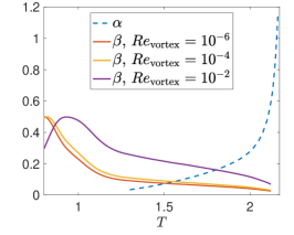
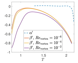
Figure 1: Dimensionless friction parameters $\alpha$ and $\beta$ (left), $\alpha^{\prime}$ and $\beta^{\prime}$ (centre) and $\Gamma$ (right) as a function of temperature $T$ and, for $\beta$ and $\beta^{\prime}$, typical vortex Reynolds numbers, defined as $Re_{\rm vortex}={|\mathbf{v}_{n_{\perp}}-\dot{\mathbf{s}}|a_{0}}/{4\nu_{n}}$.

Finally note that for a given temperature, there are two more dimensionless parameters

$$Re=\frac{v_{n}^{\rm rms}L}{\nu_{n}}\quad {\rm and} \quad I_{\rm turb}=\frac{v_{n}^{\rm rms}}{|\langle{\bf v}_{n}-{\bf v}_{s}\rangle|},$$ (31)

where $v_{n}^{\rm rms}$ is the root-mean-square or the characteristic normal fluid velocity fluctuation and $L$ is its integral scale. The Reynolds number $Re$ tells how turbulent is the normal fluid and the turbulent intensity $I_{\rm turb}$ measures the strength of thermal counterflows with respect to normal fluid turbulent fluctuations. Note that, alternatively, we can also use a Reynolds number $\displaystyle Re_{\lambda}=\frac{v_{n}^{\rm rms}\lambda_{T}}{\nu_{n}}$ based on the Taylor micro scale of the flow $\lambda_{T}$, which provides a precise definition in terms of velocity gradients and fluctuations Frisch1995 (the relation between the Taylor micro scale $\lambda_{T}$ and the the turbulent kinetic energy dissipation $\epsilon$ in homogenous and isotropic turbulence is as follows $\epsilon=15\nu_{n}(v_{n}^{\rm rms}/\lambda_{T})^{2}$ leading to $Re_{\lambda}\sim\sqrt{15}\;Re^{1/2}$).

III Numerical Method

The numerical integration of the self-consistent model Eqs. (LABEL:Eq:SelfConstModelEqVn) - (29) demands special care. In particular, the coupling between the vortex filament method and the Navier–Stokes equation requires interpolations to determine the values of the normal fluid at the filament position and a redistribution of the force $\mathbf{f}_{ns}$ onto the mesh where the normal fluid is defined. As we shall see at the end of this section, a careless treatment of the coupling may lead to spurious numerical artefacts.

In this section we describe the numerical method used to solve equations (LABEL:Eq:SelfConstModelEqVn) - (29) and provide physical and numerical justifications for the choice of the numerical scheme used to couple superfluid and normal fluid. We start by briefly describing the numerical scheme for the Vortex Filament Method and for the Navier–Stokes equations, and then proceed to the friction coupling.

III.1 Vortex Filament Method

Here we briefly describe the Vortex Filament Method (VFM) to determine the time evolution of vortex lines. For a more in-depth overview of the VFM, we point the reader to a recent review article hanninen-baggaley-2014 and references within. The underlying assumption of the VFM is that vortex lines in the superfluid component can be considered one-dimensional space curves around which the circulation is one quantum of circulation $\kappa$. This is a reasonable assumption in helium II as the vortex core size $a_{0}$ is much smaller than any other characteristic length scale of the flow. However, during the time evolution of a turbulent vortex tangle, there are important events such as vortex reconnections, during which this assumption breaks down. We shall discuss how these events can be accounted for in the VFM at the end of the section.

1. Lagrangian discretization

   At each time, we discretize the vortex tangle $\cal L$ in $N_{p}$ Lagrangian vortex points $\displaystyle\left\{\mathbf{s}_{i}(t)\right\}_{i=1,\dots,N_{p}}\;$ The distance between neighbouring points is kept in the range $[\delta/2,\delta]$ by removing or inserting additional points baggaley-barenghi-2011c . As the vortex configuration evolves, so does this Lagrangian discretisation - $N_{p}$ depends on the total length of the tangle. The vortex points evolve in time according to Eq. (19) written in dimensionless form, namely

   $$\dot{\mathbf{s}_{i}}(t)=\mathbf{v}_{s_{\perp}}(\mathbf{s}_{i},t)+\beta\;\mathbf{s}_{i}^{\prime}(t)\times\left(\mathbf{v}_{n}(\mathbf{s}_{i},t)-\mathbf{v}_{s}(\mathbf{s}_{i},t)\right)+\beta^{\prime}\;\mathbf{s}_{i}^{\prime}(t)\times\left\{\mathbf{s}_{i}^{\prime}(t)\times\left[\mathbf{v}_{n}(\mathbf{s}_{i},t)-\mathbf{v}_{s}(\mathbf{s}_{i},t)\right]\right\}\;\;,$$ (32)

   where spatial derivatives along the vortex lines are performed employing fourth-order finite difference schemes which account for the varying mesh size along the vortex lines gamet-etal-1999 ; baggaley-barenghi-2011c , and time integration is performed using the third-order Adams-Bashforth method.

   The interpolation of the normal fluid velocity $\mathbf{v}_{n}$ on each vortex point $\mathbf{s}_{i}$ presents some numerical issues; the different schemes which we have tested are outlined and discussed in Section III.3. The evaluation of the superfluid velocity $\mathbf{v}_{s}$ on the vortex points $\mathbf{s}_{i}$ via Eq. (11) must be dealt with caution as the Biot-Savart integral diverges when $\mathbf{x}\rightarrow\mathbf{s}_{i}$ in Eq. (11). This singularity is removed in a standard fashion by splitting the Biot-Savart integral into local and nonlocal contributions schwarz-1985 , that is (omitting time dependency to ease notation) by writing

   $$\mathbf{v}_{s}(\mathbf{s}_{i})=\nabla\phi(\mathbf{s}_{i})+\frac{\kappa}{4\pi}\ln\left(\frac{\sqrt{\delta_{i}\delta_{i+1}}}{a_{0}}\right)\mathbf{s}_{i}^{\prime}\times\mathbf{s}_{i}^{\prime\prime}+\frac{\kappa}{4\pi}\oint_{\mathcal{L}^{\prime}}\frac{\mathbf{s}^{\prime}(\xi)\times(\mathbf{s}_{i}-\mathbf{s}(\xi))}{|\mathbf{s}_{i}-\mathbf{s}(\xi)|^{3}}d\xi\;\;\;\;,$$ (33)

   where $\delta_{i}$ and $\delta_{i+1}$ are the lengths of the segments $[\mathbf{s}_{i-1}\,,\,\mathbf{s}_{i}]$ and $[\mathbf{s}_{i}\,,\,\mathbf{s}_{i+1}]$ respectively, $\displaystyle\mathbf{s}_{i}^{\prime\prime}=\partial^{2}\mathbf{s}(\xi,t)/\partial\xi^{2}$ evaluated at ${\mathbf{s}_{i}}$ is the normal vector to the curve in $\mathbf{s}(\xi,t)=\mathbf{s}_{i}$, and $\mathcal{L}^{\prime}$ is the vortex configuration without the section between $\mathbf{s}_{i-1}$ and $\mathbf{s}_{i+1}$. To match the periodic boundaries used in the integration of the Navier–Stokes equations for the normal fluid (Section III.2), we introduce periodic wrapping into the VFM. This involves creating copies of the vortex configuration around the original configuration; the contributions of these copies are included in the Biot-Savart integrals, Eq. (33). In order to speed-up the calculation of Biot Savart integrals for dense tangles of vortices, Eq. (33) is approximated using a tree algorithm baggaley-barenghi-2012 which scales as $N_{p}\log N_{p}$ rather than $N_{p}^{2}$.

2. Vortex reconnections

   In the limit of zero temperature, Equation (10) expresses the superfluid’s underlying incompressible, inviscid Euler dynamics in integral form saffman-1992 . Hence, on the basis of Helmholtz theorem, the topology of the superflow ought to be frozen, i.e. reconnections of vortex lines are not envisaged. We know however from experiments bewley-etal-2008 ; serafini-etal-2017 and from more microscopic models koplik-levine-1993 ; tebbs-etal-2011 ; kerr-2011 ; kursa-etal-2011 ; villois-etal-2017 ; galantucci-etal-2019 that when vortex lines come sufficiently close to each other, they reconnect, exchanging strands, as envisaged by Feynman feynman-1955 .

   In order to model vortex reconnections within the VFM, we supplement Eq. (32) with an ad-hoc algorithmical reconnection procedure. This strategy was originally proposed by Schwarz schwarz-1978 , and since then a number of alternative algorithms have been proposed. Whilst this procedure is essentially arbitrary, a number of different implementations have been extensively tested and compared baggaley-2012b , finding no significant physical difference between these implementations.

III.2 Navier Stokes Solver

We solve Eq.(LABEL:Eq:SelfConstModelEqVn) using a standard pseudo-spectral code in a three dimensional periodic domain of size $L_{x}\times L_{y}\times L_{z}$ with $n_{x},n_{y}$ and $n_{z}$ collocation points in each direction. Derivatives of the fields are directly computed in spectral space, whereas non-linear terms are evaluated in physical space. The code is de-aliased using the standard 2/3-rule, and therefore the maximum wavenumber is $k_{\rm max}=2\pi\min{[n_{x}/L_{x},n_{y}/L_{y},n_{z}/L_{z}]}/3$. The main advantage of pseudo-spectral codes is that non-linear partial differential equations are solved with spectral accuracy; this means that spatial approximation errors decrease exponentially with the number of collocation points. The drawbacks of pseudo-spectral codes are that the computational box must be periodic and Fourier transforms are intensively used.

The external forcing in Eq.(LABEL:Eq:SelfConstModelEqVn) consists of a superposition of random Fourier modes:

$${\bf F}_{\rm ext}({\bf x})=\frac{f_{0}}{{\mathcal{N}}_{f}}\sum_{k_{\rm inf}\leq|{\bf k}|\leq k_{\rm sup}}{\bf F}_{\bf k}e^{i{\bf k}\cdot{\bf x}},$$ (34)

where ${\bf F}_{\bf k}$ is a Gaussian vector of zero mean and unit variance satisfying ${\bf F}_{\bf k}\cdot{\bf k}=0$ (incompressibility condition), and ${\bf F}_{\bf k}^{*}={\bf F}_{-\bf k}$. ${\mathcal{N}}_{f}$ is a normalisation constant to impose that $\langle|{\bf F}_{\rm ext}({\bf x})|^{2}\rangle=f_{0}^{2}$. A second choice of forcing is the so-called frozen forcing. It is simply obtained (after each time step) by setting the velocity field equal to a prescribe field for wave-vectors in a predefined range. This second forcing mimics a physical forcing working at constant velocity.

The pressure in the Navier–Stokes equation ensures the incompressible condition. The condition is easily satisfied by inverting the Poisson equation

$$-\frac{1}{\rho_{n}}\nabla^{2}p=\nabla\cdot\left(\left(\mathbf{v}_{n}\cdot\nabla\right)\mathbf{v}_{n}\right)-\frac{1}{\rho_{n}}\nabla\cdot\left(\oint_{\mathcal{L}}\delta(\mathbf{x-s})\mathbf{f}_{ns}(\mathbf{s})\mathrm{d}\xi\right).$$ (35)

Let us denote by $\mathcal{P}$ the projector into the subspace of divergence-free functions, and define $P_{ij}=\delta_{ij}-\frac{\partial_{i}\partial_{j}}{\nabla^{2}}$ where $\partial_{i}=\partial/\partial x_{i}$. The equation of motion for the normal fluid simplifies to

$$\frac{\partial\mathbf{v}_{n}}{\partial t}+\mathcal{P}\left(\mathbf{v}_{n}\cdot\nabla\right)\mathbf{v}_{n}=\nu_{n}^{0}\nabla^{2}\mathbf{v}_{n}+\frac{1}{\rho_{n}}\mathcal{P}\oint_{\mathcal{L}}\delta(\mathbf{x-s})\mathbf{f}_{ns}(\mathbf{s})\mathrm{d}\xi+\frac{1}{\rho_{n}}\mathbf{F}_{\rm ext}.$$ (36)

In practice, since the projector $\mathcal{P}$ takes a trivial form in Fourier space, we directly solve Eq.(36). Note that the force acting on the normal fluid due to the interaction with the vortex lines also needs to be projected. Finally, we remark that the mean normal fluid velocity evolves in time due to the friction force as a consequence of momentum transfer between components:

$$\frac{\partial\langle\mathbf{v}_{n}\rangle}{\partial t}=\frac{1}{L_{x}L_{y}L_{z}}\frac{1}{\rho_{n}}\oint_{\mathcal{L}}\mathbf{f}_{ns}(\mathbf{s})\mathrm{d}\xi.$$ (37)

III.3 Interpolation

The equation of motion of the vortex lines, Eq. (28), needs the values of the normal fluid velocity at the Lagrangian discretization points along the vortex lines, where ${\bf v}_{n}$ is not known. In principle, as the normal fluid is periodic, any inter mesh value can be computed exactly (within spectral accuracy) by using a Fourier transform. We call this interpolation scheme Fourier interpolation and use it as benchmark for comparisons. The Fourier interpolation is extremely costly and prohibitive for practical applications, as it requires $n_{x}n_{y}n_{z}$ evaluations of complex exponentials for each Lagrangian point along the vortex lines. Affordable interpolation schemes are typically defined on physical space and their accuracy depends on the order of the method and on the regularity of the field. In three dimensions, the most commonly used schemes are Nearest neighbours, where the value of the closest grid point is taken, and Tri-Linear or Tri-Cubic interpolation, performed in each direction by a line or a cubic polynomial. More recently, a new approach based on fourth-order B-splines has been proved to be specially well adapted to pseudo-spectral codes, and found to be non-expensive and highly accurate vanHinsberg2012 .

In order to study the effect of different interpolation schemes, we study how a superfluid vortex ring moves in a static spatially dependent flow. We do not take into account yet the retroaction of the vortex filament on the normal fluid which we keep fixed. We consider a domain of size $L_{x}=L_{y}=L_{z}=2\pi$; for the normal fluid we choose the following superposition of ABC flows at different scales:

$${\bf v}_{n}(x,y,z)=\sum_{n=1}^{n_{\rm max}}(B\cos{ny}+C\sin{nz},A\sin{x}+C\cos{nz},A\cos{nx}+B\sin{ny}),$$ (38)

with $A=1,B=-1,C=5$ and $n_{\rm max}=10$. We evaluate the field on a mesh with $N=128$ and $256$ collocation points in each direction. As the largest wavevector is $\sqrt{3}\,n_{\rm max}$, the Fourier interpolation is exact (up to round-up errors).

We initialise a vortex ring of size $R=0.2387$ (in non-dimensional units) and set the temperature at $T=1.95\rm~{}K$. We let the ring evolve with the static normal fluid in the background. As the ring evolves, it deforms in the presence of the highly non-homogeneous normal fluid. In order to obtain a quantitative comparison between different schemes, we measure the average radius of the voretx ring as a function of time $R(t)=\langle|{\bf s(\xi)}-{\bf s}_{\rm center}|\rangle$ where ${\bf s}_{\rm center}=\langle{\bf s}\rangle$ and the average is performed over vortex points. The temporal evolution of $R(t)$ is displayed in Fig.2 for two different resolutions and different interpolation schemes.

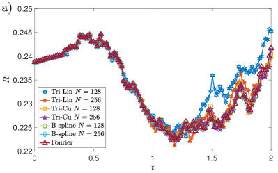
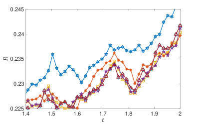
Figure 2: (Color online) Temporal evolution of the average radius of a vortex ring for different interpolation schemes and normal fluid grid resolutions (arbitrary units). The right figure displays an enlargement of the left figure at late times to better judge the interpolation schemes.

As expected, it is apparent that the error decreases when the number of collocation points of the normal fluid grid increases. It is also clear that Tri-linear interpolation gives poor results.

To better quantify the accuracy of the interpolation methods, we compute the relative error of the radius with respect to the reference radius obtained by Fourier interpolation $|R(t)-R_{\rm ref}(t)|/R_{\rm ref}(t)$. The time evolution of this relative error is displayed in Fig.3. Remarkably, the B-spline interpolation reduces the interpolating errors considerably. The extra cost of the B-spline scheme is just one single fast Fourier transform independently the number of points to be interpolated, and this is why we choose it for our local self-consistent approach, FOUCAULT.

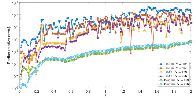
Figure 3: (Color online). Temporal evolution of the relative error $|R(t)-R_{\rm ref}(t)|/R_{\rm ref}(t)$, where the reference evolution is obtained with Fourier interpolation (arbitrary units).

III.4 Friction distribution

We now discuss the back-reaction force of the vortex lines on the normal fluid. This force, seen from the normal fluid, is $\delta$-supported on the $N_{p}$ Lagrangian points along the vortex lines $\displaystyle\left\{\mathbf{s}_{i}(t)\right\}_{i=1,\dots,N_{p}}\;$ and needs to be distributed on the grid points where the normal fluid is computed. More precisely, we denote by $(\zeta,\mu,\chi)$, with ${\zeta,\mu,\chi}\in[0,1)$, the neighboring grid points of ${\bf s}_{i}(t)$. The force ${\bf f}_{\rm ns}({\bf s}_{i}(t))$ exerted by the vortex line on the normal fluid has to be distributed among neighbouring points using weights $w_{\zeta,\mu,\chi}$, as showed schematically in Fig.4.

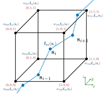
Figure 4: Sketch of the force distribution and weights.

By definition, the weights satisfy $\displaystyle\sum_{\zeta,\mu,\chi=0}^{1}w_{\zeta,\mu,\chi}=1$. In principle, extra smoothing of the force field can be applied after the force has been distributed. This numerical problem is often faced in active matter systems, where small point-like particles (i.e. swimmers, plankton, bacteria) retro-act on a classical turbulent flow. Let us rewrite the normal fluid equation considering the discretisation of the vortex lines discussed in Section III.1:

$$\frac{\partial\mathbf{v}_{n}}{\partial t}+\mathcal{P}\left(\mathbf{v}_{n}\cdot\nabla\right)\mathbf{v}_{n}=\nu_{n}^{0}\nabla^{2}\mathbf{v}_{n}+\frac{1}{\rho_{n}}\sum_{i=1}^{N_{p}}\mathcal{P}\delta(\mathbf{x}-\mathbf{s}_{i}(t))\mathbf{f}_{ns}^{\,i}(t)\delta_{i}\;\;,$$ (39)

where $\mathbf{f}_{ns}^{i}(t):={\bf f}_{\rm ns}({\bf s}_{i}(t))$, $\delta_{i}$ is the length of the $i$-th vortex line element and the dependence on time of the friction force is explicitly showed, as it will play an important role in the subsequent part of the discussion. For the sake of simplicity, the external force has been omitted in Eq. (39) and a simple Riemann sum has been used to approximate the line integral. Note that a trapezoidal rule, which is a better approximation, may be numerically used by the simple replacement $\delta_{i}\to(\delta_{i}+\delta_{i+1})/2$ and readjusting the indices of the sum. It is thus evident that our problem is formally identical to coupling discrete, point-like, active particles to the turbulent flow of a classical viscous fluid.

It is well known that in problems of active matter properties such as e.g. aggregation and condensation, mixing or/and growing of species may strongly depend on the choice of the force distribution method and the filtering scale gualtieri_picano_sardina_casciola_2015 ; GualtieriPREActiveParticlesPRE . The same issues appear in our self-consistent local model FOUCAULT. In order to illustrate this problem, we consider the simple case of a vortex ring moving in a initially quiescent normal fluid, similar to the setting studied in kivotides-barenghi-samuels-2000 . We consider a ring of radius $R=0.2387$ and set the temperature at $T=1.95^{\circ}$K. Because of friction, we expect the ring to shrink. We compare the temporal evolution of its radius employing different filtering methods. We distribute the force to the nearest neighbour grid points, i.e. $w_{\zeta,\mu,\chi}=0$ for all grid points except the nearest one to ${\bf s}_{i}$. The resulting force field is then filtered by using either a moving average over $N_{\rm filter}$ points or a Gaussian kernel of width $N_{\rm filter}\Delta x$, where $\Delta x=L_{x}/N_{x}$ is the mesh size. Figure 5 displays the temporal evolution of the vortex ring radius for the different schemes. It is clear that the shrinking rate of the radius of the ring depends strongly on the filtering procedure which is employed.

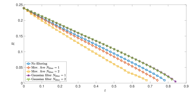
Figure 5: (Color online). Temporal evolution of the radius of a vortex ring with in an initially uniform, quiescent normal fluid. The force acting on the normal fluid is distributed to the nearest neighbour point of the mesh. Different filtering procedures are tested.

This dependence is clearly spurious. A numerical method based on physics principles is hence needed. Since our context is turbulence, it makes sense to adopt the same rigorous regularisation approach which has been used to take into account the strongly localised response of point-like particles in classical turbulence gualtieri_picano_sardina_casciola_2015 ; GualtieriPREActiveParticlesPRE . The advantage of adopting this method is that the regularisation of the exchange of momentum between point-like particles and viscous flows is based on the physics of the generation of vorticity and its viscous diffusion at very small scales. In our case, the justification of this method arises from the very small Reynolds numbers of the flow based on the vortex core radius and the small velocity of the vortex line with respect to the normal fluid.

We refer the reader to the original papers gualtieri_picano_sardina_casciola_2015 ; GualtieriPREActiveParticlesPRE for further details; in brief, this approach which we borrow from classical turbulence is based on the solution of the delta-forced, linear unsteady Stokes equation. Accordingly to the classical formulation, we introduce the time-delay $\epsilon_{R}$ coinciding with the time interval during which the localised vorticity (generated by the relative motion between the vortex line and the normal fluid) is diffused to the relevant hydrodynamic scale of the flow, the spacing $\Delta x$ of the computational grid which the normal fluid velocity field is calculated on. This finite time delay, $\epsilon_{R}$, regularises the delta-shaped nature of the friction force $\mathbf{f}_{ns}^{\,i}(t)\delta(\mathbf{x}-\mathbf{s}_{i}(t))$ in a natural way via the fundamental solution of the diffusion equation:

$$g[\mathbf{x}-\mathbf{s}_{i}(t-\epsilon_{R}),\epsilon_{R}]=\frac{1}{(4\pi\nu\epsilon_{R})^{3/2}}\exp\left[-\frac{||\mathbf{x}-\mathbf{s}_{i}(t-\epsilon_{R})||^{2}}{4\nu\epsilon_{R}}\right]\;\;,$$ (40)

This solution, Eq. (40), is a Gaussian with standard deviation $\sigma_{R}=\sqrt{2\nu\epsilon_{R}}$. The resulting expression for the friction force exerted by the $i$-th vortex line element on the normal fluid at the time $t$ at the point $\mathbf{x}$ is $\mathbf{f}_{ns}^{\,i}(t-\epsilon_{R})g[\mathbf{x}-\mathbf{s}_{i}(t-\epsilon_{R}),\epsilon_{R}]\delta_{i}$ gualtieri_picano_sardina_casciola_2015 ; GualtieriPREActiveParticlesPRE , yielding the following modified Navier–Stokes equation for the normal fluid velocity field:

$$\frac{\partial\mathbf{v}_{n}}{\partial t}+\mathcal{P}\left(\mathbf{v}_{n}\cdot\nabla\right)\mathbf{v}_{n}=\nu_{n}^{0}\nabla^{2}\mathbf{v}_{n}+\frac{1}{\rho_{n}}\sum_{i=1}^{N_{p}}\mathcal{P}\;\mathbf{f}_{ns}^{\,i}(t-\epsilon_{R})g[\mathbf{x}-\mathbf{s}_{i}(t-\epsilon_{R}),\epsilon_{R}]\delta_{i}\;\;.$$ (41)

From the physical point of view, Eq. (41) implies that the strongly localised vorticity injected in the normal flow by the relative motion of the vortices is neglected until it has been diffused by viscosity to a characteristic length scale $\sigma_{R}=\sqrt{2\nu\epsilon_{R}}$. To be consistent, and in order to take into account the vortex induced disturbances as soon as the relevant hydrodynamic scales are affected, we choose the finite time delay $\epsilon_{R}$ so that $\sigma_{R}/\Delta x=1$. Extensive tests performed in the original paper gualtieri_picano_sardina_casciola_2015 ensure that $\sigma_{R}/\Delta x=1$ is a suitable choice.

In theory, for each $i$-th vortex line element, it is possible to compute the corresponding weight for each point of the numerical grid: it would sufficient to integrate the Gaussian kernel $g[\mathbf{x}-\mathbf{s}_{i}(t-\epsilon_{R}),\epsilon_{R}]$ over the volume $\Delta V=\Delta x\Delta y\Delta z$ centred on the grid point. For instance, as displayed in the schematic two-dimensional Fig. 6, the force generated by the $i$-th vortex element at ${\bf s}_{i}$ contributes to the force computed on mesh point ${\bf x}$, but also on mesh point ${\bf z}$, the weights being the integral of $g(\mathbf{x}-\mathbf{s}_{i},\epsilon_{R})$ over their respective cells, represented by black dashed squares in the Fig. 6. This procedure would have to be repeated on each grid point for each vortex element. Although exact, this approach would be extremely costly. In addition, referring again to Fig.6, the weight corresponding to mesh point ${\bf z}$ is very small as we choose $\sigma_{R}/\Delta x=1$; the diffusion based regularisation which we employ localises in fact the force in a sphere of radius $\sigma_{R}$ centred at ${\bf s}_{i}$. As a consequence, instead of distributing the force on each grid point by computing $N_{x}\,N_{y}\,N_{z}\,N_{p}$ integrals $g(\mathbf{x}-\mathbf{s}_{i},\epsilon_{R})$ all over the grid, we distribute the force only to neighbouring mesh points of ${\bf s}_{i}$, taking care of including the weights of far grid points. Proceeding in this fashion, the total force is preserved, as the integral of $\displaystyle\int_{\mathbb{R}^{3}}g[\mathbf{x}-\mathbf{s}_{i}(t-\epsilon_{R}),\epsilon_{R}]\mathrm{d}{\bf x}=1$. As matter of example, in the sketch outlined in Fig.6, the ${\bf f}_{\rm ns}({\bf s}_{i})$ of point ${\bf s}_{i}$ will be distributed among only the four neighbouring points. In order to use a conservative scheme, for each of the neighbouring points the Gaussian kernel $g(\mathbf{x}-\mathbf{s}_{i},\epsilon_{R})$ will be integrated on the corresponding full quadrant (octant in three dimensions): in the two-dimensional simplified sketch in Fig.6, this corresponds to integrating $g$ over the region coloured in green for point ${\bf x}$ and over the yellow region for point ${\bf y}$. The generalisation to three dimension is straightforward. The advantage of this approach is that the space integrals of $g$ may actually be computed analytically.

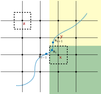
Figure 6: (Color online). Schematic two-dimensional distribution of the friction force.

The computation of the integrals leads to the weights $w_{\zeta,\mu,\chi}$ that will be used to distribute the force among the neighbouring grid points of ${\bf s}_{i}$, as illustrated in Fig.4. Note that because the Gaussian kernel $g$ is normalised to one, the requirement that $\displaystyle\sum_{\zeta,\mu,\chi=0}^{1}w_{\zeta,\mu,\chi}=1$ is satisfied by construction. To compute the weights $w_{\zeta,\mu,\chi}$, we first note that the integrals of $g(\mathbf{x}-\mathbf{s}_{i},\epsilon_{R})$ can be factorised in each Cartesian direction: we will therefore only compute the contribution in the $x$ direction, the computation of the contributions of the other directions is formally identical. The weight for the grid point of the left of $s_{i}^{x}$ (indicated with $\lfloor s_{i}^{x}\rfloor$, corresponding to $\zeta=0$) results from the one-dimensional integral over $(-\infty,\lfloor s_{i}^{x}\rfloor+\frac{\Delta x}{2})$, whereas the weight for the grid point on the right ($\lfloor s_{i}^{x}\rfloor+\Delta x$, $\zeta=1$), stems from the integral over $(\lfloor s_{i}^{x}\rfloor+\frac{\Delta x}{2},\infty)$. The calculation of the one-dimensional weight is straightforward; we have:

$$w_{\zeta}[s_{i}^{x}]=\zeta+(1-2\zeta)\frac{1}{2}\left(1+Erf{\left[-\frac{\tilde{s}_{i}^{x}-\frac{1}{2}}{\sqrt{2}(\sigma_{R}/\Delta x)}\right]}\right)$$ (42)

$$\tilde{s}_{i}^{x}=\frac{s_{i}^{x}-\lfloor s_{i}^{x}\rfloor}{\Delta x}\in[0,1].$$ (43)

The integrals $w_{\mu}[s_{i}^{y}]$ and $w_{\chi}[s_{i}^{z}]$ over the two remaining directions are performed in the same fashion. The diffusion-based weights for the three dimensional grid are finally given by

$$w_{\zeta,\mu,\chi}=w_{\zeta}[s_{i}^{x}]w_{\mu}[s_{i}^{y}]w_{\chi}[s_{i}^{z}]$$ (44)

III.5 Numerical Strategy and Parallelisation

We have implemented the numerical integration of the fully-coupled local model taking advantage of modern parallel computing. The solvers of the VFM and the Navier–Stokes equations are of very different nature, but they need to interact only through the evaluation of the friction force. In this first version of the solver, we have opted for an hybrid OpenMP-MPI parallelisation scheme. The two solvers are handled by different MPI processes. Each MPI process contains many OpenMP threads, so each solver is also independently parallelised by using this shared memory library. The evaluation of the friction force requires communication between the two solvers that do not have access to each other fields and variables. This communication is managed through the Message Passing Interface (MPI) library at the end of each time step. This scheme is naturally adapted to modern clusters that contain many nodes, with each node having a large number of CPUs with shared memory.

Finally, we remark that the values of the time step for the Navier–Stokes equations and for the VFM solver need not be the same; typically, the VFM requires a smaller time step. In order to speed up the code, depending on the physical problem, each solver can perform sub-loops (in time) to ensure numerical stability and an efficient integration of the full model.

IV Applications

In this section we show two physical applications of our fully-coupled local model FOUCAULT: (i) a superfluid vortex ring moving (i) in an initially stationary normal fluid and (ii) in a turbulent normal fluid. Our aim is not to introduce any new physical phenomena but simply validate our approach and show its computational capabilities.

1. Vortex ring in initially quiescent normal fluid

   We first study the vortex configuration investigated in the pioneer work of Kivotides et al. kivotides-barenghi-samuels-2000 : a vortex ring moving in a initially quiescent normal fluid. They observed that, due to the interaction between superfluid and normal fluid, two concentric vortex rings are created in the normal fluid, accompanying the superfluid vortex ring, forming a triple vortex structure. We integrate our fully-coupled model using as initial condition a superfluid vortex ring of radius $R=0.2387$ in a box of size $2\pi$ and set the temperature to $T=1.95\rm~{}K$.

   As the superfluid vortex ring travels, it sets in motion the surrounding normal fluid, thus losing energy and shrinking. A visualisation of the resulting flow is displayed in Fig.7. The superfluid vortex ring is displayed in green and the two normal fluid vortex rings which are generated are rendered in orange-reddish colours, forming the same triple vortex structure discovered by Kivotides et al. kivotides-barenghi-samuels-2000 . On the plane perpendicular to the vortex rings we also show the normal fluid translational velocity in the direction of propagation of the three vortex rings, rendered in blue-white colours: a wake (or jet) behind the superfluid ring, recently identified mastracci-etal-2019 , is apparent.

   

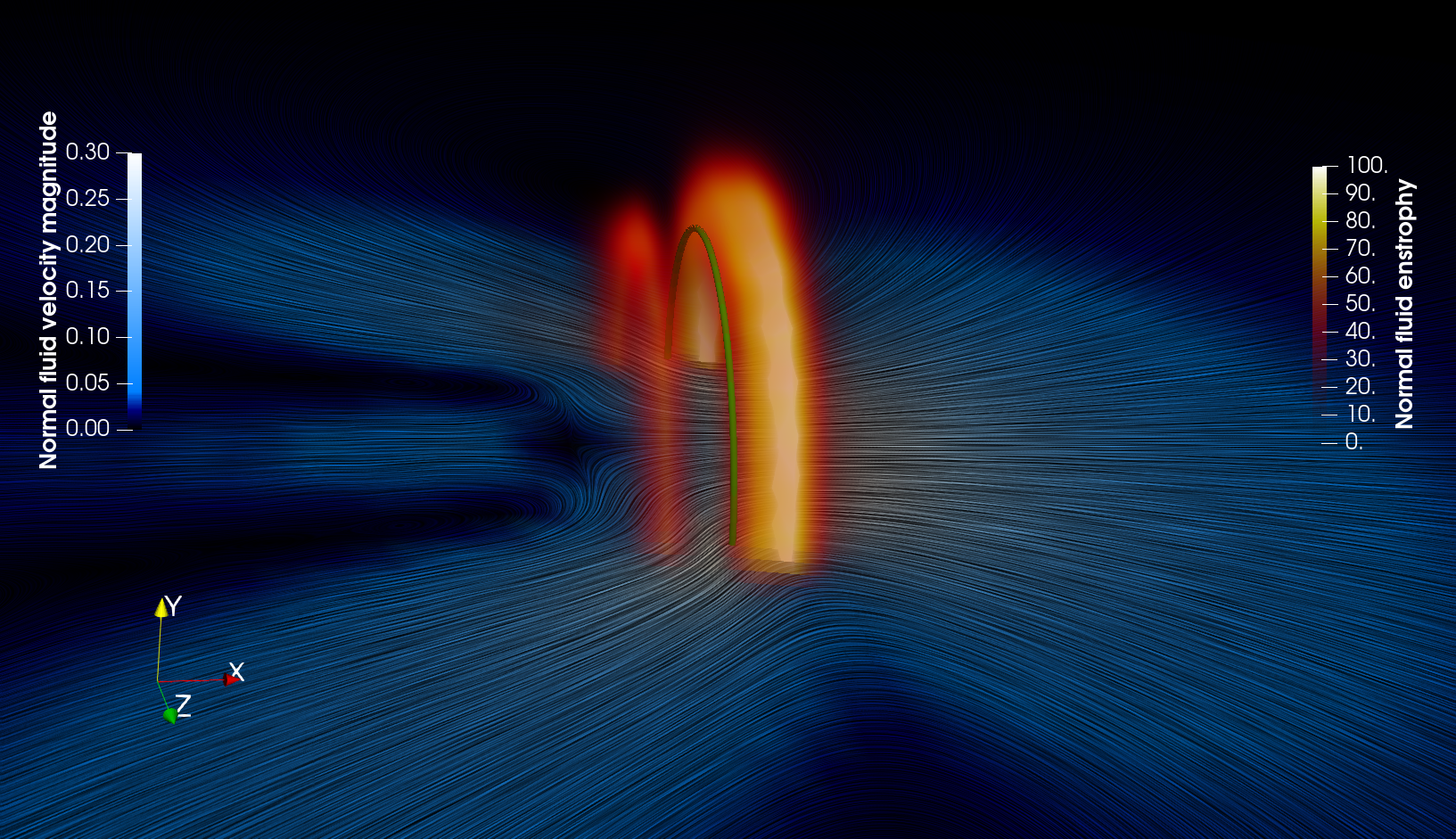
   Figure 7: (Color online). A superfluid vortex ring moving in the normal fluid initially at rest. Half of the superfluid vortex ring is visible as a green line intersecting the xy plane; the superfluid vortex ring moves to the right along the x direction. The normal fluid enstrophy is displayed by the orange-reddish-black rendering: two concentric normal fluid vortex rings are visible, slightly ahead and slightly behind the superfluid vortex ring, travelling in the same direction. The normal fluid velocity magnitude is also displayed using a black-blue-white rendering on the xy plane.

2. Vortex ring in turbulent normal fluid.

   Our second application is the effect of turbulence in the normal fluid component on the dynamics of a superfluid vortex ring. As discussed in section III.2, we can easily add an external forcing ${\bf F}_{\rm ext}$ to the Navier–Stokes equations in order to sustain the normal fluid turbulence. We first produce a turbulent state using a volumetric external forcing at large scales ($k_{\rm sup}=1$). We use a resolution of $256^{3}$ points, which allows us to obtain a Reynolds number based on the Taylor micro-scale equal to $Re_{\lambda}=127$. Once the turbulent state is prepared, we study the evolution at temperature $T=1.95\rm~{}K$ of a superfluid vortex ring of radius $R=35\eta$, where $\eta$ is the Kolmogorov length scale of the flow. The initial condition used in our self-consistent local model is displayed in Fig. 8 (top left panel).

   

   

   

   

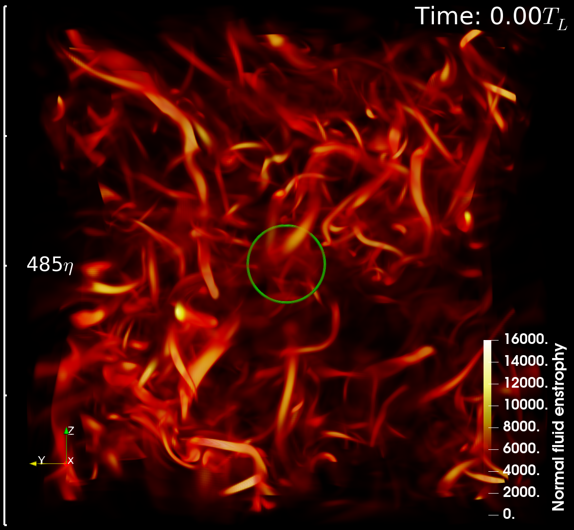
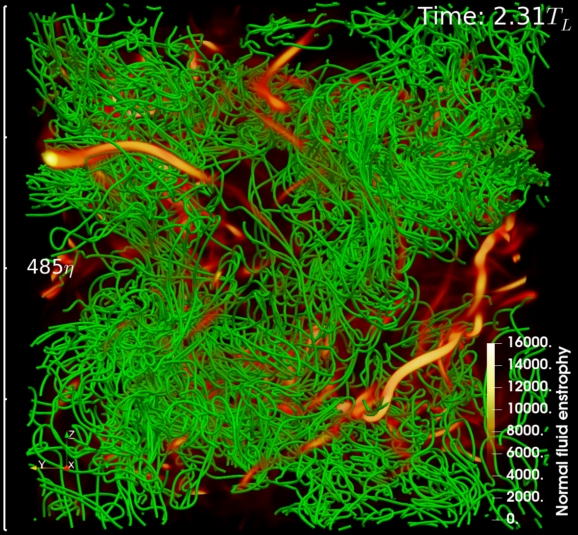
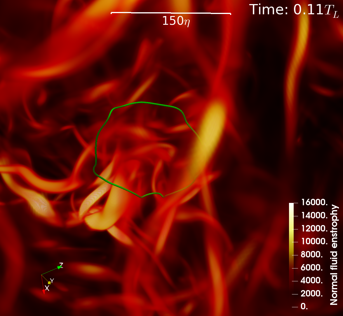
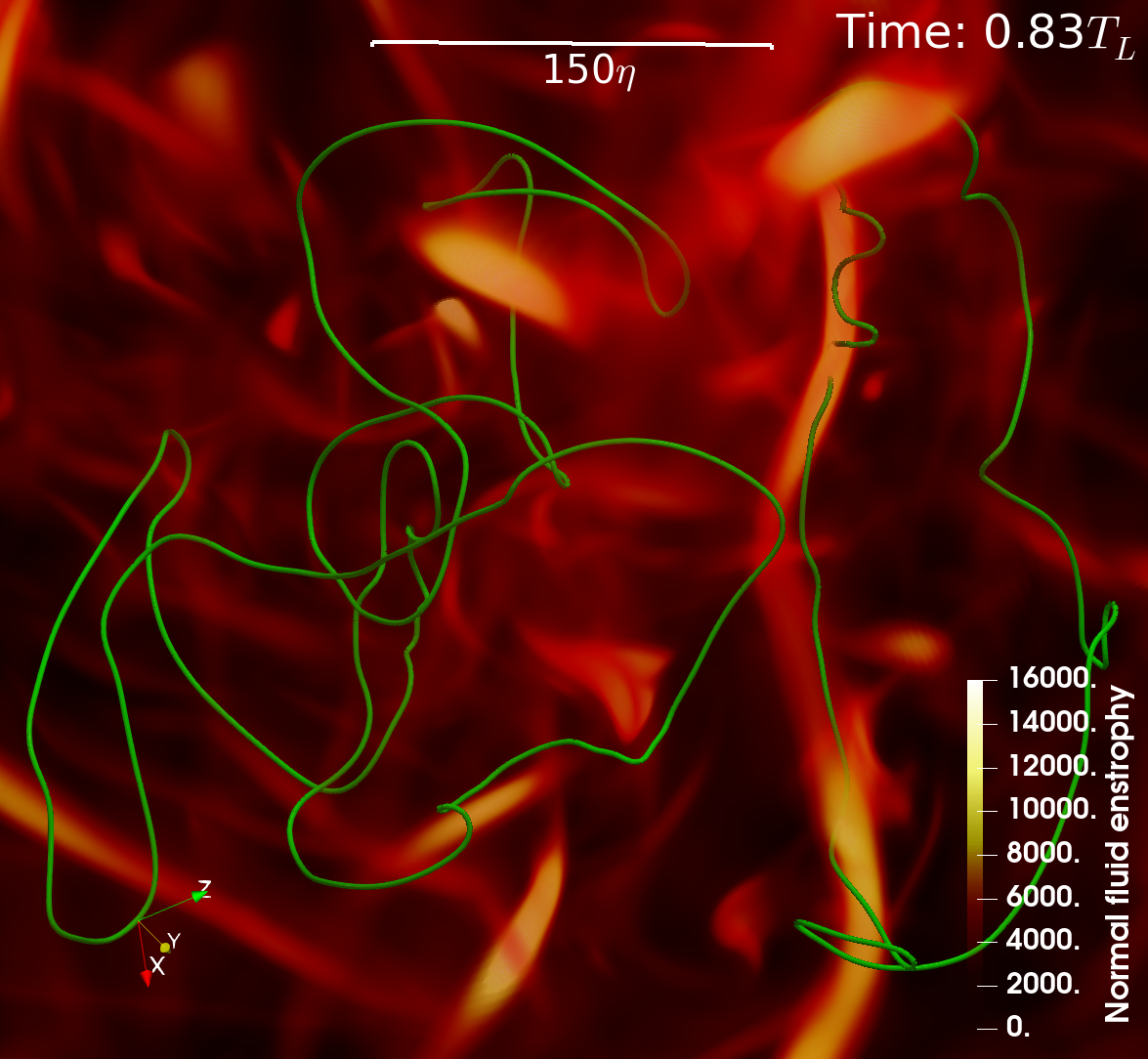
   Figure 8: (Colour online). Evolution of a superfluid vortex ring in turbulent normal fluid. The superfluid vortex ring is visualised by the green line. The normal fluid enstrophy is displayed by the yellow-orange-black rendering. The top row displays the full box at the initial (left) and the final (right) time of the simulation. The bottom row, show zoom close to the vortex ring at two early times. The figures are taken at $t=0$ (top left), $t=2.31T_{L}$ (top right), $t=0.11T_{L}$ (bottom left), and $t=0.83T_{L}$ (bottom right), where $T_{L}$ is the large eddy-turnover time of the normal fluid. The solid white lines indicate the size, expressed in units of the Kolmogorov length $\eta$ ,of the structures in the flow.

   We clearly observe the turbulent fluctuations of the normal fluid displayed by the reddish rendering of the normal fluid enstrophy. As time evolves, the turbulent fluctuations destabilise the superfluid vortex ring, inducing large amplitude Kelvin waves (bottom left panel); After a couple of large-eddy-turnover times, the vortex ring self-reconnects, forming vortex loops which undergo further reconnections, creating a turbulent superfluid vortex tangle in equilibrium with the turbulent normal fluid. It is apparent from Fig. 8 that normal fluid fluctuations are responsible for an increase of the total vortex length. In Fig.9 we display the temporal dependence of the total superfluid vortex length: the large amount of stretching is evident. The right panel shows that initially the vortex length does not increase exponentially, as predicted for the Donnelly-Glaberson instability Tsubota2003 for a uniform normal flow, but with approximate power-law character. The figure also shows that, remarkably, there is a change of behaviour at times of the order of one $T_{L}$, suggesting that normal fluid fluctuations may play an important role in quantum turbulence. This is an interesting question with important implications for current quantum turbulence experiments. It is natural to expect that the evolution of the vortex length should depend on temperature, but be independent schwarz-1988 of the initial vortex configuration. Clearly, an accurate and physically sound solver of the fully-coupled dynamics of normal fluid and superfluid like the solver that we have presented here is an important tool for the next studies of quantum turbulence.

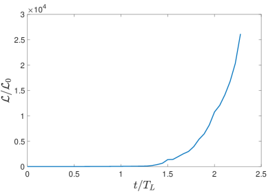
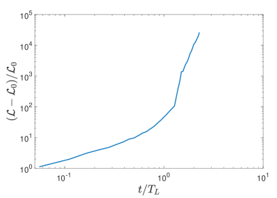
Figure 9: (Color online). Left panel: Temporal evolution of the total vortex length $\mathcal{L}$ resulting form a (initially perfect) vortex ring of length $\mathcal{L}_{0}=2\pi R\approx 1.5$ in a turbulent normal fluid background. Right panel: relative increase of the vortex length during the initial stage.

V Conclusions

We have presented a novel algorithm, named FOUCAULT, for the numerical simulations of quantum turbulence in helium II at nonzero temperatures. The main features of our approach are (i) the parallelised, efficient, pseudo-spectral code, capable of distributing the calculation amongst distinct computational cluster codes, and (ii) the forcing scheme employed for the normal fluid. These features allow the resolution a wider range of length scales compared to previous studies, from large quasi-classical scales to small quantum length scales smaller than the average inter-vortex distance. This is of fundamental importance in order to investigate the character of quantum turbulence shared with its classical counterpart, as well as the features which are specific to turbulent superfluid flows.

From the point of view of the physical modelling, a novel feature of our approach is the local computation of the friction force, stemming from classical creeping flow analysis, which (unlike previous work) is independent of the numerical discretisation on the vortex lines. In addition, our approach implements an exact regularisation of the friction force based on the small-scale viscous diffusion of the disturbances generated by vortex lines moving with respect to the normal fluid.

After a detailed description of the distinct features of our algorithm, we have applied it to two problems: the motion of a superfluid vortex ring in an initially stationary normal fluid and in a turbulent normal fluid. In the first problem we have recovered the same qualitative features (the double normal ring structure and wake) observed in previous work; in the second we have demonstrated a new effect - the vortex stretching induced by turbulent fluctuations.

In conclusion, our novel algorithm paves the way for a new series of investigations of quantum turbulence in helium II at finite temperatures, particularly at length scales smaller than the average inter-vortex spacing in problems where the singular and quantised nature of the superfluid vortices is expected to play a fundamental role.

References

- (1) WF Vinen and JJ Niemela. Quantum turbulence. J Low Temp Phys, 128:167, 2002.
- (2) L Skrbek and KR Sreenivasan. Developed quantum turbulence and its decay. Phys Fluids, 24:011301, 2012.
- (3) CF Barenghi, L Skrbek, and KR Sreenivasan. Introduction to quantum turbulence. Proc Natl Acad Sci USA, 111:supp 1, 4647, 2014.
- (4) LP Pitaevskii and S Stringari. Bose-Einstein condensation. Oxford University Press, 2003.
- (5) CF Barenghi and NG Parker. A Primer on Quantum Fluids. Springer, Heidelberg 2016
- (6) L Tisza. Transport phenomena in helium II. Nature, 141:913, 1938.
- (7) LD Landau. Theory of the superfluidity of helium ii. J. Phys U.S.S.R., 5:71, 1941.
- (8) SR Stalp, L Skrbek, and RJ Donnelly. Phys Rev Lett, 82:4831, 1999.
- (9) J Maurer and P Tabeling. Local investigation of superfluid turbulence. Europhys Lett, 43:29, 1998.
- (10) J Salort, C Baudet, B Castaing, B Chabaud, F Daviaud, T Didelot, P Diribarne, B Dubrulle, Y Gagne, F Gauthier, A Girard, B Henbral, B Rousset, P Thibault, and PE Roche. Turbulent velocity spectra in superfluid flows. Phys Fluids, 22:125102, 2010.
- (11) CF Barenghi, V L’vov, and PE Roche. Experimental, numerical and analytical velocity spectra in turbulent quantum fluid. Proc Natl Acad Sci USA, 111:supp 1, 4683, 2014.
- (12) VS L’vov, S Nazarenko, and L Skrbek. Energy spectra of developed turbulence in helium superfluids. J Low Temp Phys, 145:125, 2006.
- (13) VS L’vov, S Nazarenko, and O Rudenko. Gradual eddy-wave crossover in superfluid turbulence. J Low Temp Phys, 153:150, 2008.
- (14) AW Baggaley, J Laurie, and CF Barenghi. Vortex-density fluctuations, energy spectra, and vortical regions in superfluid turbulence. Phys Rev Lett, 109:205304, 2012.
- (15) AW Baggaley and CF Barenghi. Vortex-density fluctuations in quantum turbulence. Phys Rev B, 84:020504, 2011.
- (16) T Araki, M Tsubota, and SK Nemirovskii. Energy spectrum of superfluid turbulence with no normal-fluid component. Phys Rev Lett, 89:145301, 2002.
- (17) M Kobayashi and M Tsubota. Kolmogorov spectrum of superfluid turbulence: Numerical analysis of the Gross-Pitaevskii equation with a small-scale dissipation. Phys Rev Lett, 94:065302, 2005.
- (18) M La Mantia, D Duda, M Rotter, and L Skrbek. Lagrangian accelerations of particles in superfluid turbulence. J Fluid Mech, 717:R9, 2013.
- (19) M La Mantia. Particle dynamics in wall-bounded thermal counterflow of superfluid helium. Phys Fluids, 29:065102, 2017.
- (20) WF Vinen. Mutual friction in a heat current in liquid helium ii. i. experiments on steady heat currents. Proc Roy Soc London A, 240:114, 1957.
- (21) CF Barenghi, YA Sergeev, and AW Baggaley. Regimes of turbulence without an energy cascade. Sci Rep, 6:35701, 2017.
- (22) T Zhang and SW Van Sciver. Large-scale turbulent flow around a cylinder in counterflow superfluid4He (he II). Nat Phys, 1:36, 2005.
- (23) GP Bewley, DP Lathrop, and KR Sreenivasan. Visualization of quantized vortices. Nature, 441:588, 2006.
- (24) M La Mantia, TV Chagovets, M Rotter, and L Skrbek. Testing the performance of a cryogenic visualization system on thermal counterflow by using hydrogen and deuterium solid tracers. Rev Sci Instr, 83:055109, 2012.
- (25) W Guo, SB Cahn, JA Nikkel, WF Vinen, and DN McKinsey. Visualization study of counterflow in superfluid helium-4 using metastable helium molecules. Phys Rev Lett, 105:045301, 2010.
- (26) R Hänninen and AW Baggaley. Vortex filament method as a tool for computational visualization of quantum turbulence. Proc Natl Acad Sci USA, 111: supp 1, 4667, 2014.
- (27) L Galantucci, M Sciacca, and CF Barenghi. Coupled normal fluid and superfluid profiles of turbulent helium ii in channels. Phys Rev B, 92:174530, 2015.
- (28) L Galantucci, M Sciacca, and CF Barenghi. Large-scale normal fluid circulation in helium superflows. Phys Rev B, 95:014509, 2017.
- (29) S Yui, M Tsubota, and H Kobayashi. Three-dimensional coupled dynamics of the two-fluid model in superfluid he 4: Deformed velocity profile of normal fluid in thermal counterflow. Phys Rev Lett, 120:155301, 2018.
- (30) D Kivotides, CF Barenghi, and DC Samuels. Triple vortex ring structure in superfluid helium ii. Science, 290:777, 2000.
- (31) OC Idowu, A Willis, CF Barenghi, and DC Samuels. Local normal-fluid helium ii flow due to mutual friction interaction with the superfluid. Phys Rev B, 62:3409, 2000.
- (32) D Kivotides. Decay of finite temperature superfluid helium-4 turbulence. J Low Temp Phys, 181:68, 2015.
- (33) D Kivotides. Superfluid helium-4 hydrodynamics with discrete topological defects. Phys Rev F, 3:104701, 2018.
- (34) P Gualtieri, F Picano, G Sardina, and CM Casciola. Exact regularized point particle method for multiphase flows in the two-way coupling regime. J Fluid Mech, 773:520, 2015.
- (35) P Gualtieri, F Battista, and CM Casciola. Turbulence modulation in heavy-loaded suspensions of tiny particles. Phys. Rev. Fluids, 2:034304, 2017.
- (36) D Kivotides. Spreading of superfluid vorticity clouds in normal-fluid turbulence. J Fluid Mech, 668:58, 2011.
- (37) F London. Superfluids, volume 2. Wiley, New York, 1954.
- (38) RJ Donnelly. Quantized Vortices in Helium II. Cambridge University Press, 1991.
- (39) SK Nemirovskii. Quantum turbulence: Theoretical and numerical problems. Phys Report, 524:85, 2013.
- (40) HE Hall and WF Vinen. The rotation of liquid helium ii. i. experiments on the propagation of secound sound in uniformly rotating helium ii. Proc Roy Soc London A, 238:204, 1956.
- (41) HE Hall and WF Vinen. The rotation of liquid helium II. (ii) the theory of mutual friction in uniformly rotating helium. Proc Roy Soc London A, 238:215, 1956.
- (42) P Švančara and M La Mantia. Flight-crash events in superfluid turbulence. J Fluid Mech, 876: R2, 2019.
- (43) B Mastracci, S Bao, W Guo, and WF Vinen. Particle tracking velocimetry applied to thermal counterflow in superfluid he 4: Motion of the normal fluid at small heat fluxes. Phys Rev Fluids, 4:083305, 2019.
- (44) RK Childers and JT Tough. Helium II thermal counterflow: Temperature- and pressure- difference data and analysis in terms of the vinen theory. Phys Rev B, 13:1040, 1976.
- (45) IL Bekarevich and IM Khalatnikov. Phenomenological derivation of the equations of vortex motion in he II. Sov Phys JETP, 13:643, 1961.
- (46) CF Barenghi and CA Jones. The stability of the Couette flow of helium II. J Fluid Mech 197:551, 1988.
- (47) CF Barenghi. Vortices and the Couette flow of helium II. Phy. Rev B 45:2290, 1992.
- (48) KL Henderson, CF Barenghi, and CA Jones. Taylor-Couette flow of helium II. J Fluid Mech 283:329, 1995.
- (49) PE Roche, CF Barenghi and E Leveque. Quantum turbulence at finite temperature. The two fluid cascade. Europhys Lett 87:54006, 2009.
- (50) RN Hills and PH Roberts. Superfluid mechanics for a high density of vortex lines. Arch Rat Mech Anal, 66:43, 1977.
- (51) KW Schwarz. Turbulence in superfluid helium: steady homogenous counterflow. Phys Rev B, 18(1):245, 1978.
- (52) KW Schwarz. Three-dimensional vortex dynamics in superfluid he 4: Line-line and line-boundary interactions. Phys Rev B, 31(9):5782, 1985.
- (53) KW Schwarz. Three-dimensional vortex dynamics in superfluid he4. Phys Rev B, 38(4):2398, 1988.
- (54) H Adachi, S Fujiyama, and M Tsubota. Steady-state counterflow quantum turbulence: Simulation of vortex filaments using the full biot-savart law. Phys Rev B, 81:104511, 2010.
- (55) AW Baggaley, LK Sherwin, CF Barenghi, and YA Sergeev. Thermally and mechanically driven quantum turbulence in helium ii. Phys Rev B, 86:104501, 2012.
- (56) LK Sherwin-Robson, CF Barenghi, and AW Baggaley. Local and nonlocal dynamics in superfluid turbulence. Phys Rev B, 91:104517, 2015.
- (57) RGKM Aarts and ATAM de Waele. Numerical investigation of the flow properties of he ii. Phys Rev B, 50:10069, 1994.
- (58) AW Baggaley and S Laizet. Vortex line density in counterflowing he ii with laminar and turbulent normal fluid velocity profiles. Phys Fluids, 25:115101, 2013.
- (59) D Khomenko, L Kondaurova, VS L’vov, P Mishra, A Pomyalov, and I Procaccia. Dynamics of the density of quantized vortex–lines in superfluid turbulence. Phys Rev B, 91:180504(R), 2015.
- (60) AW Baggaley and J Laurie. Thermal counterflow in a periodic channel with solid boundaries. J Low Temp Phys, 178:35–52, 2015.
- (61) S Yui and M Tsubota. Counterflow quantum turbulence of he–ii una square channel: Numerical analysis with nonuniform flows of the normal fluid. Phys Rev B, 91:184504, 2015.
- (62) DC Samuels. Response of superfluid vortex filaments to concentrated normal-fluid vorticity. Phys Rev B, 47(2):1107, 1993.
- (63) CF Barenghi, DC Samuels, G Bauer, and RJ Donnelly. Superfluid vortex lines in a model turbulent flow. Phys Fluids, 9:2631, 1997.
- (64) D Kivotides. Coherent structure formation in turbulent thermal superfluids. Phys Rev Lett, 96:175301, 2006.
- (65) K Morris, J Koplik, and DWI Rouson. Vortex locking in direct numerical simulations of quantum turbulence. Phys Rev Lett, 101:015301, 2008.
- (66) OC Idowu, D Kivotides, CF Barenghi, and DC Samuels. Equation for self-consistent superfluid vortex line dynamics. J Low Temp Phys, 120:269, 2000.
- (67) D Kivotides. Turbulence without inertia in thermally excited superfluids. Phys Lett A, 341:193, 2005.
- (68) D Kivotides. Relaxation of superfluid vortex bundles via energy transfer to the normal fluid. Phys Rev B, 76:054503, 2007.
- (69) D Kivotides. Energy spectra of finite temperature superfluid helium-4 turbulence. Phys Fluids, 26:105105, 2014.
- (70) D Kivotides. Interactions between normal-fluid and superfluid vortex rings in helium-4. EPL, 112:36005, 2015.
- (71) S Kaplun and PA Lagerstrom. Asymptotic expansions of navier-stokes solutions for small reynolds numbers. J Maths and Mechanics, 6:585, 1957.
- (72) S Kaplun. Low Reynolds number flow past a circular cylinder. J Maths and Mechanics, 6:595, 1957.
- (73) I Proudman and JRA Pearson. Expansions at small reynolds numbers for the flow past a sphere and a circular cylinder. J Fluid Mech, 2:237, 1957.
- (74) M Van Dyke. Perturbation methods in fluid mechanics. Parabolic Press, Stanford, California, 1975.
- (75) CF Barenghi, WF Vinen and RJ Donnelly, Friction on quantized vortices in helium II: a review. J Low Temp Phy., 52: 189, 1982.
- (76) GE Volovik. Three nondissipative forces on a moving vortex line in superfluids and superconductors. JETP LETTERS, 62:1, 1995.
- (77) L Thompson and PCE Stamp. Quantum dynamics of a bose superfluid vortex. Phys Rev Lett, 108:184501, 2012.
- (78) RJ Donnelly and CF Barenghi. The observed properties of liquid helium at the saturated vapor pressure. J Phys Chem Ref Data, 27:1217, 1998.
- (79) Uriel Frisch. Turbulence: The Legacy of AN Kolmogorov. Cambridge University Press, 1995.
- (80) AW Baggaley and CF Barenghi. Spectrum of turbulent kelvin-waves cascade in superfluid helium. Phys Rev B, 83:134509, 2011.
- (81) L Gamet, F Ducros, F Nicoud, and T Poinsot. Compact finite difference schemes on non-uniform meshes. application to direct numerical simulations of compressible flows. Int J Num Meth Fluids, 29(2):159, 1999.
- (82) AW Baggaley and CF Barenghi. Tree method for quantum vortex dynamics. J Low Temp Phys, 166:3, 2012.
- (83) PG Saffman. Vortex dynamics. Cambridge University Press, 1992.
- (84) GP Bewley, MS Paoletti, KR Sreenivasan, and DP Lathrop. Characterization of reconnecting vortices in superfluid helium. Proc Natl Acad Sci USA, 105:13707, 2008.
- (85) S Serafini, L Galantucci, E Iseni, T Bienaime, R Bisset, CF Barenghi, F Dalfovo, G Lamporesi, and G Ferrari. Vortex reconnections and rebounds in trapped atomic bose-einstein condensates. Phys Rev X, 7:021031, 2017.
- (86) J Koplik and H Levine. Vortex reconnection in superfluid helium. Phys Rev Lett, 71:1375, 1993.
- (87) R Tebbs, A J. Youd, and CF Barenghi. The approach to vortex reconnection. J Low Temp Phys, 162:314, 2011.
- (88) RM Kerr. Vortex stretching as a mechanism for quantum kinetic energy decay. Phys Rev Lett, 106:224501, 2011.
- (89) M Kursa, K Bajer, and T Lipniaki. Cascade of vortex loops initiated by a single reconnection of quantum vortices. Phys Rev B, 83:014515, 2011.
- (90) A Villois, D Proment, and G Krstulovic. Universal and nonuniversal aspects of vortex reconnections in superfluids. Phys Rev Fluids, 2:044701, 2017.
- (91) L Galantucci, M Sciacca, and D Jou. The two fluid extended model of superfluid helium. Atti Accad Pelorit Pericol Cl Sci Fis Mat Nat, 97:A4, 2019.
- (92) RP Feynmann. Application of quantum mechanics to liquid helium, ed by Gorter. vol 1, chapter II, page 36. N Holland Publ Co, 1955.
- (93) AW Baggaley. The sensitivity of the vortex filament method to different reconnection models. J Low Temp Phys, 168:18, 2012.
- (94) M. van Hinsberg, JT Boonkkamp, F Toschi, and H Clercx. On the efficiency and accuracy of interpolation methods for spectral codes. SIAM J Sci Comput, 34:B479, 2012.
- (95) M Tsubota, T Araki, and CF Barenghi. Rotating superfluid turbulence. Phys Rev Lett 90:205301, 2003.
- (96) JS Brooks and RJ Donnelly. The calculated thermodynamic properties of superfluid helium-4. J Phys Chem Ref Data 6:51, 1977.