A Note on Portfolio Optimization
with Quadratic Transaction Costs

Abstract

In this short note, we consider mean-variance optimized portfolios with transaction costs. We show that introducing quadratic transaction costs makes the optimization problem more difficult than using linear transaction costs. The reason lies in the specification of the budget constraint, which is no longer linear. We provide numerical algorithms for solving this issue and illustrate how transaction costs may considerably impact the expected returns of optimized portfolios.

Keywords: Portfolio allocation, mean-variance optimization, transaction cost, quadratic programming, alternating direction method of multipliers.

JEL classification: C61, G11.

1 Introduction

The general approach for introducing liquidity management in the mean-variance optimization model of Markowitz (1952) is to assume fixed bid-ask spreads. We then obtain the linear transaction cost model, which can be solved using an augmented quadratic programming problem (Scherer, 2007). However, as shown by Lecesne and Roncoroni (2019a, 2019b), unit transaction costs may be a linear function of the trading size, implying that a model with quadratic transaction costs may be more appropriate. In this article, we investigate this approach and show how linear and quadratic transaction costs modify the mean-variance optimized framework. In particular, we do not obtain a standard QP problem when transaction costs are quadratic, because the budget constraint is no longer linear. In this case, we obtain a quadratically constrained quadratic program (QCQP), which is an NP-hard problem. However, using the ADMM framework, we are able to derive an efficient algorithm that solves this issue. Finally, we use this algorithm to illustrate the impact of transaction costs on optimized portfolios and Markowitz efficient frontiers.

2 Introducing transaction costs into portfolio optimization

2.1 Mean-variance optimization with transaction costs

We consider a universe of $n$ assets. Let $w=\left(w_{1},\ldots,w_{n}\right)$ be a portfolio. The return of Portfolio $w$ is given by:

$$R\left(w\right)=\sum_{i=1}^{n}w_{i}R_{i}=w^{\top}R$$

where $R=\left(R_{1},\ldots,R_{n}\right)$ is the random vector of asset returns. If we note $\mu$ and $\Sigma$ the vector of expected returns and the covariance matrix of asset returns, we deduce that the expected return of Portfolio $w$ is equal to:

$$\mu\left(w\right)=\mathbb{E}\left[R\left(w\right)\right]=w^{\top}\mu$$

whereas its variance is given by:

$$\sigma^{2}\left(w\right)=\mathbb{E}\left[\left(R\left(w\right)-\mu\left(w\right)\right)^{2}\right]=w^{\top}\Sigma w$$

The mean-variance optimization framework of Markowitz (1952) consists in maximizing the expected return $\mu\left(w\right)$ for a fixed value $\sigma^{\star}$ of the volatility $\sigma\left(w\right)$. This can be achieved by maximizing the quadratic utility function:

$$\mathcal{U}\left(w\right)=\gamma\mu\left(w\right)-\frac{1}{2}\sigma^{2}\left(w\right)$$

The mean-variance optimization framework can then be rewritten as a standard quadratic programming (QP) problem:

$$w^{\star} = \arg\min\frac{1}{2}w^{\top}\Sigma w-\gamma w^{\top}\mu$$ (1)

$$\mathrm{s.t.} \left\{\begin{array}[]{l}\mathbf{1}_{n}^{\top}w=1\\ \mathbf{0}_{n}\leq w\leq\mathbf{1}_{n}\end{array}\right.$$ (4)

The budget constraint $\mathbf{1}_{n}^{\top}w=1$ (or $\sum_{i=1}^{n}w_{i}=1$) implies that the wealth is entirely invested, whereas the second constraint indicates that Portfolio $w$ is long-only.

Let us now introduce transaction costs. We note $\tilde{w}$ the current portfolio and $\mathcal{C}\left(w\mid\tilde{w}\right)$ the cost of rebalancing the current portfolio $\tilde{w}$ towards the portfolio $w$. We deduce that the net return is equal to the gross return minus the transaction costs:

$$R\left(w\mid\tilde{w}\right)=R\left(w\right)-\mathcal{C}\left(w\mid\tilde{w}\right)$$

It follows that:

$$\mu\left(w\mid\tilde{w}\right) = \mathbb{E}\left[R\left(w\mid\tilde{w}\right)\right]$$

$$= \mu\left(w\right)-\mu_{\mathcal{C}}\left(w\mid\tilde{w}\right)$$

and:

$$\sigma^{2}\left(w\mid\tilde{w}\right) = \mathbb{E}\left[\left(R\left(w\mid\tilde{w}\right)-\mu\left(w\mid\tilde{w}\right)\right)^{2}\right]$$

$$= \mathbb{E}\left[\left(R\left(w\right)-\mu\left(w\right)+\mu_{\mathcal{C}}\left(w\mid\tilde{w}\right)-\mathcal{C}\left(w\mid\tilde{w}\right)\right)^{2}\right]$$

$$= \sigma^{2}\left(w\right)+\sigma_{\mathcal{C}}^{2}\left(w\mid\tilde{w}\right)-2\rho_{\mathcal{C}}\left(w\mid\tilde{w}\right)\sigma\left(w\right)\sigma_{\mathcal{C}}\left(w\mid\tilde{w}\right)$$

where $\mu_{\mathcal{C}}\left(w\mid\tilde{w}\right)=\mathbb{E}\left[\mathcal{C}\left(w\mid\tilde{w}\right)\right]$ is the expected cost of rebalancing and $\sigma_{\mathcal{C}}\left(w\mid\tilde{w}\right)$ is the standard deviation of $\mathcal{C}\left(w\mid\tilde{w}\right)$. The function $\rho_{\mathcal{C}}\left(w\mid\tilde{w}\right)$ is the correlation between the gross return $R\left(w\right)$ and the transaction cost $\mathcal{C}\left(w\mid\tilde{w}\right)$. Generally, we assume that $\rho_{\mathcal{C}}\left(w\mid\tilde{w}\right)\approx 0$. We notice that transaction costs impact both the expected return and the volatility of the portfolio. However, this is not the only effect. Indeed, we also have to finance the rebalancing process since the wealth before and after is not the same. Therefore, the budget constraint becomes:

$$\mathbf{1}_{n}^{\top}w+\mathcal{C}\left(w\mid\tilde{w}\right)=1$$

Here, we face an issue because the budget constraint is stochastic. This is why portfolio managers assume that transaction costs are known and not random. In this case, the optimization problem becomes:

$$w^{\star} = \arg\min\frac{1}{2}w^{\top}\Sigma w-\gamma\left(w^{\top}\mu-\mathcal{C}\left(w\mid\tilde{w}\right)\right)$$ (5)

$$\mathrm{s.t.} \left\{\begin{array}[]{l}\mathbf{1}_{n}^{\top}w+\mathcal{C}\left(w\mid\tilde{w}\right)=1\\ \mathbf{0}_{n}\leq w\leq\mathbf{1}_{n}\end{array}\right.$$ (8)

2.2 Specification of transaction costs

A first idea is to consider constant transaction costs. In this case, we have:

$$\mathcal{C}\left(w\mid\tilde{w}\right)=\sum_{i=1}^{n}c_{i}\cdot\left|w_{i}-\tilde{w}_{i}\right|$$

where $c_{i}$ is the unit cost associated with Asset $i$. A better formulation is to distinguish bid and ask prices. Following Scherer (2007), we have:

$$\mathcal{C}\left(w\mid\tilde{w}\right) = \mathcal{C}^{-}\left(w\mid\tilde{w}\right)+\mathcal{C}^{+}\left(w\mid\tilde{w}\right)$$

$$= \sum_{i=1}^{n}c_{i}^{-}\cdot\max\left(\tilde{w}_{i}-w_{i},0\right)+\sum_{i=1}^{n}c_{i}^{+}\cdot\max\left(w_{i}-\tilde{w}_{i},0\right)$$

where $c_{i}^{-}$ and $c_{i}^{+}$ are the bid and ask unit transaction costs. We deduce that the transaction cost for Asset $i$ satisfies:

$$\mathcal{C}_{i}\left(w\mid\tilde{w}\right)=\left\{\begin{array}[]{ll}c_{i}^{-}\cdot\left(\tilde{w}_{i}-w_{i}\right)&\text{if }w_{i}<\tilde{w}_{i}\\ 0&\text{if }w_{i}=\tilde{w}_{i}\\ c_{i}^{+}\cdot\left(w_{i}-\tilde{w}_{i}\right)&\text{if }w_{i}>\tilde{w}_{i}\end{array}\right.$$ (9)

In this approach, the unit transaction cost is fixed and does not depend on the rebalancing weight:

$$c_{i}\left(w\mid\tilde{w}\right)=\frac{\mathcal{C}_{i}\left(w\mid\tilde{w}\right)}{\left|w_{i}-\tilde{w}_{i}\right|}=\left\{\begin{array}[]{ll}c_{i}^{-}&\text{if }w_{i}<\tilde{w}_{i}\\ 0&\text{if }w_{i}=\tilde{w}_{i}\\ c_{i}^{+}&\text{if }w_{i}>\tilde{w}_{i}\end{array}\right.$$

We can also assume that the unit transaction cost is a linear function of the rebalancing weight:

$$c_{i}\left(w\mid\tilde{w}\right)=\left\{\begin{array}[]{ll}c_{i}^{-}+\delta_{i}^{-}\cdot\left(\tilde{w}_{i}-w_{i}\right)&\text{if }w_{i}<\tilde{w}_{i}\\ 0&\text{if }w_{i}=\tilde{w}_{i}\\ c_{i}^{+}+\delta_{i}^{+}\cdot\left(w_{i}-\tilde{w}_{i}\right)&\text{if }w_{i}>\tilde{w}_{i}\end{array}\right.$$

It follows that:

$$\mathcal{C}_{i}\left(w\mid\tilde{w}\right)=\left\{\begin{array}[]{ll}c_{i}^{-}\cdot\left(\tilde{w}_{i}-w_{i}\right)+\delta_{i}^{-}\cdot\left(\tilde{w}_{i}-w_{i}\right)^{2}&\text{if }w_{i}<\tilde{w}_{i}\\ 0&\text{if }w_{i}=\tilde{w}_{i}\\ c_{i}^{+}\cdot\left(w_{i}-\tilde{w}_{i}\right)+\delta_{i}^{+}\cdot\left(w_{i}-\tilde{w}_{i}\right)^{2}&\text{if }w_{i}>\tilde{w}_{i}\end{array}\right.$$ (10)

In the academic literature, Specification (9) is known under the term ‘linear transaction costs’, whereas Specification (10) corresponds to ‘quadratic transaction costs’. An example is provided in Figure 1, where bid and ask transaction costs are different. On the left side, we have reported the linear case, whereas the quadratic case corresponds to the right side. We notice that introducing quadratic costs has a more adverse effect on the portfolio’s return. By construction, the choice of one specification will impact portfolio optimization, especially if the rebalancing is significant.

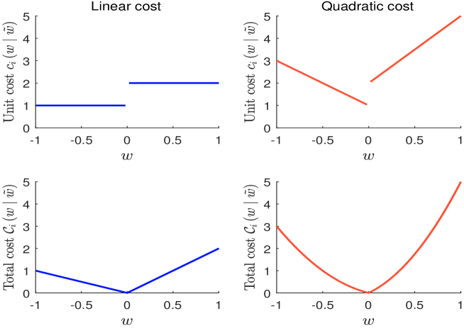
Figure 1: An example of linear and transaction costs (in %)

3 The case of linear transaction costs

3.1 The augmented QP solution

Since $\mathcal{C}\left(w\mid\tilde{w}\right)$ is a nonlinear function of $w$, Problem (5) is not a standard QP problem. This is why Scherer (2007) suggested rewriting the transaction costs as follows:

$$\mathcal{C}\left(w\mid\tilde{w}\right)=c_{i}^{-}\cdot\Delta w_{i}^{-}+c_{i}^{+}\cdot\Delta w_{i}^{+}$$

where $\Delta w_{i}^{-}=\max\left(\tilde{w}_{i}-w_{i},0\right)$ and $\Delta w_{i}^{+}=\max\left(w_{i}-\tilde{w}_{i},0\right)$ represent the sale and purchase of Asset $i$. By definition, we have $\Delta w_{i}^{-}\cdot\Delta w_{i}^{+}=0$ and:

$$w_{i}=\tilde{w}_{i}+\Delta w_{i}^{+}-\Delta w_{i}^{-}$$

We deduce that Problem (5) becomes:

$$w^{\star} = \arg\min\frac{1}{2}w^{\top}\Sigma w-\gamma\left(\sum_{i=1}^{n}w_{i}\cdot\mu_{i}-\sum_{i=1}^{n}\Delta w_{i}^{-}\cdot c_{i}^{-}-\sum_{i=1}^{n}\Delta w_{i}^{+}\cdot c_{i}^{+}\right)$$ (11)

$$\mathrm{s.t.} \left\{\begin{array}[]{l}\sum_{i=1}^{n}w_{i}+\sum_{i=1}^{n}\Delta w_{i}^{-}\cdot c_{i}^{-}+\sum_{i=1}^{n}\Delta w_{i}^{+}\cdot c_{i}^{+}=1\\ w_{i}+\Delta w_{i}^{-}-\Delta w_{i}^{+}=\tilde{w}_{i}\\ \mathbf{0}_{n}\leq w\leq\mathbf{1}_{n}\end{array}\right.$$ (15)

We notice that we obtain a QP problem with respect to the variables $x=\left(w,\Delta w^{-},\Delta w^{+}\right)$. Indeed, we have:

$$x^{\star} = \arg\min\frac{1}{2}x^{\top}Qx-x^{\top}R$$ (16)

$$\mathrm{s.t.} \left\{\begin{array}[]{l}Ax=B\\ x^{-}\leq x\leq x^{+}\end{array}\right.$$ (19)

where:

$$Q=\left(\begin{array}[]{ccc}\Sigma&\mathbf{0}_{n,n}&\mathbf{0}_{n,n}\\ \mathbf{0}_{n,n}&\mathbf{0}_{n,n}&\mathbf{0}_{n,n}\\ \mathbf{0}_{n,n}&\mathbf{0}_{n,n}&\mathbf{0}_{n,n}\end{array}\right)$$

and:

$$R=\gamma\left(\begin{array}[]{c}\mu\\ -c^{-}\\ -c^{+}\end{array}\right)$$

For the equality constraint, we obtain:

$$A=\left(\begin{array}[]{ccc}\mathbf{1}_{n}^{\top}&\left(c^{-}\right)^{\top}&\left(c^{+}\right)^{\top}\\ I_{n}&I_{n}&-I_{n}\end{array}\right)$$

and:

$$B=\left(\begin{array}[]{c}1\\ \tilde{w}\end{array}\right)$$

For the bounds, we notice that:

$$0\leq w_{i}\leq 1 \Leftrightarrow 0\leq\tilde{w}_{i}+\Delta w_{i}^{+}-\Delta w_{i}^{-}\leq 1$$

$$\Leftrightarrow -\tilde{w}_{i}\leq\Delta w_{i}^{+}-\Delta w_{i}^{-}\leq 1-\tilde{w}_{i}$$

$$\Leftrightarrow \left\{\begin{array}[]{ll}-\tilde{w}_{i}\leq\Delta w_{i}^{+}\leq 1-\tilde{w}_{i}&\text{if }\Delta w_{i}^{-}=0\\ \tilde{w}_{i}-1\leq\Delta w_{i}^{-}\leq\tilde{w}_{i}&\text{if }\Delta w_{i}^{+}=0\end{array}\right.$$

However, we know that $\Delta w_{i}^{-}\geq 0$ and $\Delta w_{i}^{+}\geq 0$. We deduce that $x^{-}=\mathbf{0}_{3n}$ and:

$$x^{+}=\left(\begin{array}[]{c}\mathbf{1}_{n}\\ \tilde{w}\\ \mathbf{1}_{n}-\tilde{w}\end{array}\right)$$

Problem (16) is called an augmented QP problem (Roncalli, 2013), because we have augmented the number of variables in order to find the optimal solution $w^{\star}$ which is given by the following relationship:

$$w^{\star}=\left(\begin{array}[]{ccc}I_{n}&\mathbf{0}_{n,n}&\mathbf{0}_{n,n}\end{array}\right)x^{\star}$$

3.2 The efficient frontier with linear transaction costs

We consider an investment universe of $7$ assets. Their expected return and volatility expressed as a $\%$ are equal to:

$$i$$ 1 2 3 4 5 6 7

1.00 2.00 3.00 4.00 5.00 7.50 10.00

1.00 2.00 3.00 4.00 5.00 7.50 10.00

We also consider a constant correlation matrix of $25\%$ between asset returns. The initial portfolio is composed of $50\%$ of Asset 1 and $50\%$ of Asset 2.

By assuming fixed transaction costs $c^{-}=20$ bps and $c^{+}=10$ bps, we obtain the efficient frontier that is reported in Figure 2. Here, we face an issue because transaction costs imply that $\sum_{i=1}^{n}w_{i}^{\star}<1$. Therefore, the efficient frontier cannot be represented by the pair $\left(\sigma\left(w^{\star}\right),\mu\left(w^{\star}\right)\right)$ because the net wealth $\sum_{i=1}^{n}w_{i}^{\star}$ depends on the values taken by $c^{-}$ and $c^{+}$. With no transaction costs, we retrieve the classical efficient frontier of Markowitz (1952). However, in order to compare efficient frontiers, we have to normalize the optimized portfolio:

$$\bar{w}^{\star}=\frac{w_{i}^{\star}}{\sum_{i=1}^{n}w_{i}^{\star}}$$

Indeed, plotting $\left(\sigma\left(w^{\star}\right),\mu\left(w^{\star}\right)\right)$ is misleading since we have paid transaction costs in order to rebalance the portfolio. For instance, if the transaction costs are high, we have $\sum_{i=1}^{n}w_{i}^{\star}\ll 1$ and we may obtain a very low volatility and some optimized portfolios may be on the left of the Markowitz efficient frontier. The reason is that the portfolio is less risky on a nominal basis because the portfolio notional is reduced. This is why it is better to consider the expected return adjusted by the transaction costs (also called the ‘net expected return’), which is equal to $\mu_{\mathrm{net}}\left(\bar{w}^{\star}\right)=\mu\left(\bar{w}^{\star}\right)-\mathcal{C}\left(w^{\star}\mid\tilde{w}\right)$. The efficient frontier with transaction costs is then represented by the curve $\left(\sigma\left(\bar{w}^{\star}\right),\mu_{\mathrm{net}}\left(\bar{w}^{\star}\right)\right)$. However, with $c^{-}=20$ bps and $c^{+}=10$ bps, Figure 2 gives the impression that transaction costs have little impact on the efficient frontier.

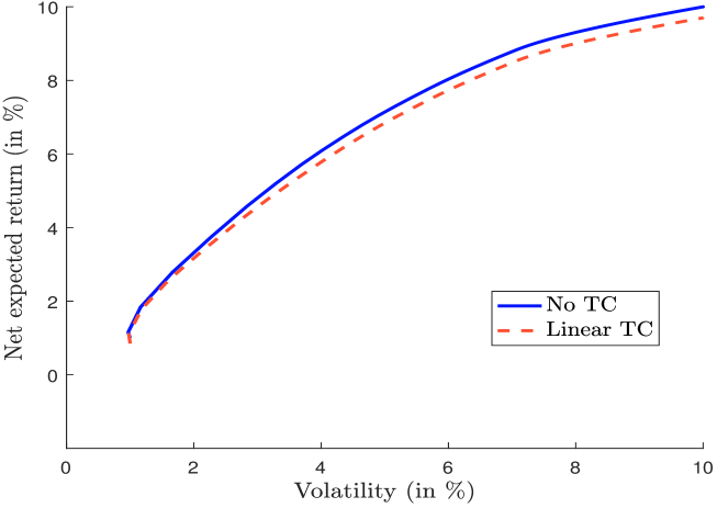
Figure 2: Efficient frontier $\left(\sigma\left(\bar{w}^{\star}\right),\mu_{\mathrm{net}}\left(\bar{w}^{\star}\right)\right)$ with $c^{-}=20$ bps and $c^{+}=10$ bps

Figure 3: Efficient frontier $\left(\sigma\left(\bar{w}^{\star}\right),\mu_{\mathrm{net}}\left(\bar{w}^{\star}\right)\right)$ with $c^{-}=2\%$ and $c^{+}=1\%$

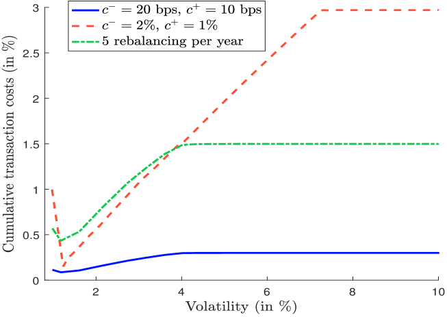
Figure 4: Transaction cost

Let us now consider an unrealistic case: $c^{-}=2\%$ and $c^{+}=1\%$. We obtain Figure 3 and we notice the big impact of transaction costs on the expected return of the portfolio. In Figure 4, we have reported the total amount of transaction costs with respect to portfolio volatility. Since the case $c^{-}=20$ bps and $c^{+}=10$ bps is more realistic, it may not reflect the real impact on a trading strategy. Indeed, these transaction costs are paid at each rebalancing date. The efficient frontier considers a yearly expected return, whereas the net expected return assumes only one portfolio rebalancing in the year, and does not take into account the total turnover of the portfolio. For example, if we assume that we rebalance the portfolio $5$ times in the year, we obtain the green curve that illustrates how cumulative transaction costs can be damaging for portfolio performance.

4 Introducing quadratic transaction costs

4.1 The issue of the quadratic budget constraint

In the case of quadratic transaction costs, we can use the same approach by considering augmented variables. We deduce that:

$$\mathcal{C}\left(w\mid\tilde{w}\right) = \sum_{i=1}^{n}\Delta w_{i}^{-}\left(c_{i}^{-}+\delta_{i}^{-}\Delta w_{i}^{-}\right)+\sum_{i=1}^{n}\Delta w_{i}^{+}\left(c_{i}^{+}+\delta_{i}^{+}\Delta w_{i}^{+}\right)$$

$$= \Delta w^{-\top}c^{-}+\Delta w^{-\top}\Delta^{-}\Delta w^{-}+\Delta w^{+\top}c^{+}+\Delta w^{+\top}\Delta^{+}\Delta w^{+}$$

where $\Delta^{-}=\mathop{\rm diag}\left(\delta_{1}^{-},\ldots,\delta_{n}^{-}\right)$ and $\Delta^{+}=\mathop{\rm diag}\left(\delta_{1}^{+},\ldots,\delta_{n}^{+}\right)$ are two diagonal matrices. It follows that the objective function of Problem (5) remains quadratic:

$$f\left(w,\Delta w^{-},\Delta w^{+}\right) = \frac{1}{2}w^{\top}\Sigma w-\gamma\left(w^{\top}\mu-\mathcal{C}\left(w\mid\tilde{w}\right)\right)$$

$$= \frac{1}{2}\left(w^{\top}\Sigma w+\Delta w^{-\top}\left(2\gamma\Delta^{-}\right)\Delta w^{-}+\Delta w^{+\top}\left(2\gamma\Delta^{+}\right)\Delta w^{+}\right)-$$

$$\gamma\left(w^{\top}\mu-\Delta w^{-\top}c^{-}-\Delta w^{+\top}c^{+}\right)$$

but the budget constraint is no longer linear:

$$\underset{\text{Linear term}}{\underbrace{\mathbf{1}_{n}^{\top}w+\Delta w^{-\top}c^{-}+\Delta w^{+\top}c^{+}}}+\underset{\text{Quadratic term}}{\underbrace{\Delta w^{-\top}\Delta^{-}\Delta w^{-}+\Delta w^{+\top}\Delta^{+}\Delta w^{+}}}=1$$

Indeed, the budget constraint is composed of a linear term and a quadratic term.

Let $x=\left(w,\Delta w^{-},\Delta w^{+}\right)$ be the vector of original variables and augmented variables. We obtain:

$$x^{\star} = \arg\min\frac{1}{2}x^{\top}Qx-x^{\top}R$$ (21)

$$\mathrm{s.t.} \left\{\begin{array}[]{l}A_{1}x+x^{\top}C_{1}x=B_{1}\\ A_{2}x=B_{2}\\ x^{-}\leq x\leq x^{+}\end{array}\right.$$ (25)

where:

$$Q=\left(\begin{array}[]{ccc}\Sigma&\mathbf{0}_{n,n}&\mathbf{0}_{n,n}\\ \mathbf{0}_{n,n}&2\gamma\Delta^{-}&\mathbf{0}_{n,n}\\ \mathbf{0}_{n,n}&\mathbf{0}_{n,n}&2\gamma\Delta^{+}\end{array}\right)$$

and:

$$R=\gamma\left(\begin{array}[]{c}\mu\\ -c^{-}\\ -c^{+}\end{array}\right)$$

For the equality constraints, we obtain:

$$\left(\begin{array}[]{c}A_{1}\\ A_{2}\end{array}\right)=\left(\begin{array}[]{ccc}\mathbf{1}_{n}^{\top}&\left(c^{-}\right)^{\top}&\left(c^{+}\right)^{\top}\\ I_{n}&I_{n}&-I_{n}\end{array}\right)$$

and:

$$\left(\begin{array}[]{c}B_{1}\\ B_{2}\end{array}\right)=\left(\begin{array}[]{c}1\\ \tilde{w}\end{array}\right)$$

The matrix $C_{1}$ is defined as follows:

$$C_{1}=\left(\begin{array}[]{ccc}\mathbf{0}_{n,n}&\mathbf{0}_{n,n}&\mathbf{0}_{n,n}\\ \mathbf{0}_{n,n}&\Delta^{-}&\mathbf{0}_{n,n}\\ \mathbf{0}_{n,n}&\mathbf{0}_{n,n}&\Delta^{+}\end{array}\right)$$

The bounds remain the same. We have $x^{-}=\mathbf{0}_{3n}$ and:

$$x^{+}=\left(\begin{array}[]{c}\mathbf{1}_{n}\\ \tilde{w}\\ \mathbf{1}_{n}-\tilde{w}\end{array}\right)$$

Again, the optimal solution $w^{\star}$ is given by the following relationship:

$$w^{\star}=\left(\begin{array}[]{ccc}I_{n}&\mathbf{0}_{n,n}&\mathbf{0}_{n,n}\end{array}\right)x^{\star}$$

4.2 The ADMM solution

Following Perrin and Roncalli (2019), we can use the alternating direction method of multipliers (ADMM) algorithm formulated by Gabay and Mercier (1976) to solve Problem (21) and overcome the non linear constraint. To do this, we leave the objective function as well as all the linear constraints in the $x$-update and put the non linear constraint in the $y$-update. In this case, the $x$-update is easily solved using QP, but the $y$-update is an NP-hard problem in the general case.

4.2.1 The ADMM formulation

Problem (21) is equivalent to:

$$\left\{x^{\star},y^{\star}\right\} = \arg\min_{\left(x,y\right)}f_{x}\left(x\right)+f_{y}\left(y\right)$$

s.t. $$x-y=\mathbf{0}_{n}$$

where:

$$f_{x}\left(x\right)=\frac{1}{2}x^{\top}Qx-x^{\top}R+\mathds{1}_{\Omega_{x}}(x)$$

and:

$$f_{y}\left(y\right)=\mathds{1}_{\Omega_{y}}(y)$$

The sets $\Omega_{x}$ and $\Omega_{y}$ are defined as follows:

$$\Omega_{x}\left(x\right)=\left\{x\in\left[0,1\right]^{n}:A_{2}x=B_{2},x^{-}\leq x\leq x^{+}\right\}$$

and:

$$\Omega_{y}\left(y\right)=\left\{y\in\left[0,1\right]^{n}:A_{1}y+y^{\top}C_{1}y=B_{1}\right\}$$

The corresponding ADMM algorithm consists of the following three steps (Boyd et al., 2011; Perrin and Roncalli, 2019):

1. The $x$-update is:

   $$x^{\left(k+1\right)}=\arg\min_{x}\left\{f_{x}\left(x\right)+\frac{\varphi}{2}\left\|x-y^{\left(k\right)}+u^{\left(k\right)}\right\|_{2}^{2}\right\}$$ (27)

2. The $y$-update is:

   $$y^{\left(k+1\right)}=\arg\min_{y}\left\{f_{y}\left(y\right)+\frac{\varphi}{2}\left\|x^{\left(k+1\right)}-y+u^{\left(k\right)}\right\|_{2}^{2}\right\}$$ (28)

3. The $u$-update is:

   $$u^{\left(k+1\right)}=u^{\left(k\right)}+x^{\left(k+1\right)}-y^{\left(k+1\right)}$$ (29)

As noted by Perrin and Roncalli (2019), the $x$-update is a QP problem:

$$x^{\left(k+1\right)} = \arg\min\frac{1}{2}x^{\top}\left(Q+\varphi I_{3n}\right)x-x^{\top}\left(R+\varphi\left(y^{\left(k\right)}-u^{\left(k\right)}\right)\right)$$ (30)

$$\mathrm{s.t.} \left\{\begin{array}[]{l}A_{2}x=B_{2}\\ x^{-}\leq x\leq x^{+}\end{array}\right.$$ (33)

There is no difficulty in finding the numerical solution $x^{\left(k+1\right)}$. In fact, the issue concerns the calculation of $y^{\left(k+1\right)}$.

4.2.2 The case $\delta_{i}^{-}=\delta^{-}$ and $\delta_{i}^{+}=\delta^{+}$

Generally, the $y$-update is easily solved by combining proximal operators and the Dykstra algorithm. However, in our case, we cannot use such a decomposition because the constraint is unusual. In fact, we have the following optimization problem:

$$y^{(k+1)} = \arg\min_{y}\frac{1}{2}\left\|y-v_{y}^{\left(k+1\right)}\right\|_{2}^{2}$$

s.t. $$y\in\Omega_{y}$$

where $v_{y}^{\left(k+1\right)}=x^{\left(k+1\right)}+u^{\left(k\right)}$. We deduce that the Lagrange function is equal to:

$$\mathcal{L}\left(y,\lambda\right) = \frac{1}{2}\left\|y-v_{y}^{\left(k+1\right)}\right\|_{2}^{2}+$$

$$\lambda\left(\sum_{i=1}^{n}\left(w_{i}+\Delta w_{i}^{-}\left(c_{i}^{-}+\delta_{i}^{-}\Delta w_{i}^{-}\right)+\Delta w_{i}^{+}\left(c_{i}^{+}+\delta_{i}^{+}\Delta w_{i}^{+}\right)\right)-1\right)$$

Using the similar partition $v_{y}^{\left(k+1\right)}=\left(v,\Delta v^{-},\Delta v^{+}\right)$ as $y=\left(w,\Delta w^{-},\Delta w^{+}\right)$, the KKT conditions are:

$$\left\{\begin{array}[]{l}w_{i}-v_{i}+\lambda=0\\ \Delta w_{i}^{-}-\Delta v_{i}^{-}+\lambda\left(c_{i}^{-}+2\delta_{i}^{-}\Delta w_{i}^{-}\right)=0\\ \Delta w_{i}^{+}-\Delta v_{i}^{+}+\lambda\left(c_{i}^{+}+2\delta_{i}^{+}y_{i}^{+}\right)=0\\ \sum_{i=1}^{n}\left(w_{i}+\Delta w_{i}^{-}\left(c_{i}^{-}+\delta_{i}^{-}\Delta w_{i}^{-}\right)+\Delta w_{i}^{+}\left(c_{i}^{+}+\delta_{i}^{+}\Delta w_{i}^{+}\right)\right)=1\end{array}\right.$$

We then get a nonlinear system of $3n+1$ equations. We first consider the case $\delta_{i}^{-}=\delta^{-}$ and $\delta_{i}^{+}=\delta^{+}$. In Appendix A.1 on page A.1, we show that $\lambda$ is the solution of a quintic equation:

$$\alpha_{5}\lambda^{5}+\alpha_{4}\lambda^{4}+\alpha_{3}\lambda^{3}+\alpha_{2}\lambda^{2}+\alpha_{1}\lambda+\alpha_{0}=0$$

From this, we can conclude that there are as many solutions to the nonlinear system as there are real roots to the last polynomial equation. Since we know that KKT conditions are necessary, it is sufficient to compare the different solutions obtained for this system in order to find the solution of our original program. More general methods are available in order to numerically solve the nonlinear system such as the Newton-Raphson algorithm. However, for these methods, it is usually necessary to compute the inverse of a Hessian matrix at each step of iteration which is very costly (around $\mathcal{O}\left((3n+1)^{3}\right)$). By taking advantage of the derivation of the $y$-update, we only need one step of cost $\mathcal{O}\left(5^{3}\right)$ to compute the roots of the polynomial in order to solve the system.

4.2.3 The case $\delta_{i}^{-}\neq\delta_{j}^{-}$ and $\delta_{i}^{+}\neq\delta_{j}^{+}$

The case $\delta_{i}^{-}\neq\delta_{j}^{-}$ and $\delta_{i}^{+}\neq\delta_{j}^{+}$ complicates the problem. Indeed, we obtain a polynomial equation of degree $2n+1$. Another solution is to rewrite the $y$-update problem in a matrix form:

$$y^{\left(k+1\right)} = \arg\min\frac{1}{2}\left(y-v_{y}^{\left(k+1\right)}\right)^{\top}\left(y-v_{y}^{\left(k+1\right)}\right)$$

$$\mathrm{s.t.} A_{1}y+y^{\top}C_{1}y-B_{1}=0$$

We obtain a quadratically constrained quadratic program (QCQP). Since a quadratic equality is not convex, the optimization problem is not convex. More generally, a QCQP is an NP-hard problem. A numerical solution is therefore to consider an interior-point algorithm by specifying the gradient of the objective function, the gradient of the equality constraint and the Hessian of the Lagrangian. However, since we have only one constraint and the objective function is simple, we can derive the numerical solution (Park and Boyd, 2017), which is described in Appendix A.2 on page A.2.

Remark 1.

The ADMM formulation has allowed us to split the QCQP Problem (21) with two inequality and two equality constraints into a QP problem ($x$-update) and a QCQP problem with only one constraint ($y$-update). As explained by Park and Boyd (2017), solving QCQP with one constraint is feasible and relatively easy. This is not always the case when there are two or more constraints.

4.3 The efficient frontier with quadratic transaction costs

We consider our previous example. We assume that the current portfolio is the optimal portfolio $\tilde{w}$ corresponding to volatility of $2\%$. In a second period, the portfolio manager would increase portfolio risk and target volatility equal to $4\%$. Portfolio $w_{\mathrm{MVO}}^{\star}$ is the optimal solution if we do not take into account transaction costs. However, this portfolio is not realistic if we consider transaction costs. We set $c^{-}=2\%$, $c^{+}=1\%$, $\delta^{-}=5\%$ and $\delta^{+}=5\%$. The results are given in Table 1. In the case of linear transaction costs, we obtain Portfolio $w_{\mathrm{LC}}^{\star}$. We observe that the two solutions $w_{\mathrm{MVO}}^{\star}$ and $w_{\mathrm{LC}}^{\star}$ are very different. For instance, the LC solution keeps a significant proportion of Asset 2 in order to pay less transaction costs. Indeed, Portfolios $w_{\mathrm{MVO}}^{\star}$ and $w_{\mathrm{LC}}^{\star}$ pay respectively $1.58\%$ and $0.98\%$ of transaction costs. In the case of quadratic transaction costs, the solution is Portfolio $w_{\mathrm{QC}}^{\star}$. We notice that it has a lower turnover than the two previous portfolios. Moreover, it selects assets with a high return in order to compensate for the transaction costs. This is why we obtain a weight of $29.13\%$ for Asset 7.

Table 1: Comparison of optimized portfolios with linear and quadratic costs

Asset	$\tilde{w}$	$w_{\mathrm{MVO}}^{\star}$	$w_{\mathrm{LC}}^{\star}$	$w_{\mathrm{QC}}^{\star}$	$\bar{w}_{\mathrm{LC}}^{\star}$	$\bar{w}_{\mathrm{QC}}^{\star}$
$1$	$26.16$	$0.01$	$0.00$	$6.70$	$0.00$	$6.80$
$2$	$21.41$	$0.08$	$14.52$	$10.84$	$14.67$	$11.01$
$3$	$16.13$	$10.92$	$16.13$	$14.32$	$16.28$	$14.53$
$4$	$12.79$	$22.42$	$12.79$	$12.78$	$12.91$	$12.98$
$5$	$10.56$	$24.77$	$10.56$	$10.56$	$10.67$	$10.72$
$6$	$7.34$	$22.59$	$18.27$	$14.17$	$18.45$	$14.38$
$7$	$5.62$	$19.22$	$26.74$	$29.13$	$27.01$	$29.57$
$\mu\left(w\right)$	$3.33$	$6.08$	$5.86$	$5.73$	$5.92$	$5.82$
$\sigma\left(w\right)$	$2.00$	$4.00$	$4.00$	$4.00$	$4.04$	$4.06$
$\mathcal{C}_{\mathrm{LC}}\left(w\mid\tilde{w}\right)$		$1.58$	$0.98$	$0.94$
$\mathcal{C}_{\mathrm{QC}}\left(w\mid\tilde{w}\right)$		$2.52$	$1.63$	$1.49$
$\mu_{\mathrm{LC}}\left(w\mid\tilde{w}\right)$	$3.33$	$4.50$	$4.88$	$4.79$
$\mu_{\mathrm{QC}}\left(w\mid\tilde{w}\right)$	$3.33$	$3.56$	$4.23$	$4.24$

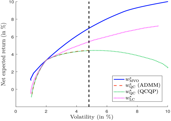
Figure 5: Efficient frontier $\left(\sigma\left(\bar{w}^{\star}\right),\mu_{\mathrm{net}}\left(\bar{w}^{\star}\right)\right)$ with quadratic transaction costs

In Figure 5, we have reported the efficient frontier with the previous transaction costs. We verify that it is below the unconstrained MVO efficient frontier. We also notice that quadratic transaction costs have a significant adverse effect on the net expected return of optimized portfolios. In our example, we rebalance a portfolio, which has low volatility. This implies that it is inefficient to target an optimized portfolio with high volatility, because we have to pay substantial transaction costs. For instance, it is impossible to target an expected return greater than $4\%$, implying that having portfolio volatility higher than $5\%$ is not optimal.

Remark 2.

We do not say that it is impossible to target volatility higher than $5\%$, but we say that it is not optimal. Indeed, the ADMM algorithm stops before the optimized portfolio reaches $5\%$. In order to match volatility $\sigma^{\star}>5\%$, we have to solve the strict $\sigma$-problem:

$$w^{\star} = \arg\max\sum_{i=1}^{n}w_{i}\cdot\mu_{i}-\sum_{i=1}^{n}\Delta w_{i}^{-}\left(c_{i}^{-}+\delta_{i}^{-}\Delta w_{i}^{-}\right)-\sum_{i=1}^{n}\Delta w_{i}^{+}\left(c_{i}^{+}+\delta_{i}^{+}\Delta w_{i}^{+}\right)$$ (34)

$$\mathrm{s.t.} \left\{\begin{array}[]{l}\sum_{i=1}^{n}w_{i}+\sum_{i=1}^{n}\Delta w_{i}^{-}\left(c_{i}^{-}+\delta_{i}^{-}\Delta w_{i}^{-}\right)+\sum_{i=1}^{n}\Delta w_{i}^{+}\left(c_{i}^{+}+\delta_{i}^{+}\Delta w_{i}^{+}\right)=1\\ w_{i}+\Delta w_{i}^{-}-\Delta w_{i}^{+}=\tilde{w}_{i}\\ \sqrt{w^{\top}\Sigma w}=\sigma^{\star}\\ \mathbf{0}_{n}\leq w\leq\mathbf{1}_{n}\end{array}\right.$$ (39)

This can be done by rewriting Problem (34) as a QCQP program. In Figure 5, we verify that QCQP optimized portfolios such that $\sigma\left(w^{\star}\right)>5\%$ are in fact not optimal, because they are dominated by portfolios with a higher expected return and lower volatility.

5 Conclusion

In this short note, we study mean-variance optimized portfolios with linear and quadratic transaction costs. We show how the problem can be solved using the techniques of quadratic programming and alternating direction method of multipliers. We also illustrate how linear and quadratic transaction costs can lead to different solutions and penalize the portfolio’s return. Moreover, the introduction of quadratic transaction costs opens a new field of research when we consider transition management, asset ramp-up or portfolio scaling.

Appendix

Appendix A Mathematical results

A.1 Solution of the $y$-update in the case $\delta_{i}^{-}=\delta^{-}$ and $\delta_{i}^{+}=\delta^{+}$

We would like to solve the following nonlinear system of $3n+1$ equations:

$$\left\{\begin{array}[]{l}w_{i}-v_{i}+\lambda=0\\ \Delta w_{i}^{-}-\Delta v_{i}^{-}+\lambda\left(c_{i}^{-}+2\delta^{-}\Delta w_{i}^{-}\right)=0\\ \Delta w_{i}^{+}-\Delta v_{i}^{+}+\lambda\left(c_{i}^{+}+2\delta^{+}\Delta w_{i}^{+}\right)=0\\ \sum_{i=1}^{n}\left(w_{i}+\Delta w_{i}^{-}\left(c_{i}^{-}+\delta^{-}\Delta w_{i}^{-}\right)+\Delta w_{i}^{+}\left(c_{i}^{+}+\delta^{+}\Delta w_{i}^{+}\right)\right)=1\end{array}\right.$$

The first $3n$ equations are equivalent to:

$$\left\{\begin{array}[]{l}w_{i}=v_{i}-\lambda\\ \Delta w_{i}^{-}=\dfrac{\Delta v_{i}^{-}-\lambda c_{i}^{-}}{\lambda^{-}}\\ \Delta w_{i}^{+}=\dfrac{\Delta v_{i}^{+}-\lambda c_{i}^{+}}{\lambda^{+}}\end{array}\right.$$

where $\lambda^{-}=1+2\lambda\delta^{-}$ and $\lambda^{+}=1+2\lambda\delta^{+}$. The last equation then becomes:

$$(\ast) \Leftrightarrow \sum_{i=1}^{n}\left(v_{i}-\lambda\right)+\sum_{i=1}^{n}\left(\frac{\Delta v_{i}^{-}-\lambda c_{i}^{-}}{\lambda^{-}}\right)\left(c_{i}^{-}+\delta_{i}^{-}\frac{\Delta v_{i}^{-}-\lambda c_{i}^{-}}{\lambda^{-}}\right)+$$

$$\sum_{i=1}^{n}\left(\frac{\Delta v_{i}^{+}-\lambda c_{i}^{+}}{\lambda^{+}}\right)\left(c_{i}^{+}+\delta_{i}^{+}\frac{\Delta v_{i}^{+}-\lambda c_{i}^{+}}{\lambda^{+}}\right)=1$$

$$\Leftrightarrow \lambda^{-^{2}}\lambda^{+^{2}}\left(\sum_{i=1}^{n}v_{i}-1\right)-\lambda\lambda^{-^{2}}\lambda^{+^{2}}n+$$

$$\lambda^{-}\lambda^{+^{2}}\sum_{i=1}^{n}c_{i}^{-}\left(\Delta v_{i}^{-}-\lambda c_{i}^{-}\right)+\lambda^{+^{2}}\delta^{-}\sum_{i=1}^{n}\left(\Delta v_{i}^{-}-\lambda c_{i}^{-}\right)^{2}+$$

$$\lambda^{-^{2}}\lambda^{+}\sum_{i=1}^{n}c_{i}^{+}\left(\Delta v_{i}^{+}-\lambda c_{i}^{+}\right)+\lambda^{-^{2}}\delta^{+}\sum_{i=1}^{n}\left(\Delta v_{i}^{+}-\lambda c_{i}^{+}\right)^{2}=0$$

We have $\lambda^{-^{2}}=\left(4\delta^{-^{2}}\right)\lambda^{2}+\left(4\delta^{-}\right)\lambda+1$, $\lambda^{+^{2}}=\left(4\delta^{+^{2}}\right)\lambda^{2}+\left(4\delta^{+}\right)\lambda+1$ and:

$$\lambda^{-}\lambda^{+^{2}} = \left(8\delta^{-}\delta^{+^{2}}\right)\lambda^{3}+4\delta^{+}\left(2\delta^{-}+\delta^{+}\right)\lambda^{2}+2\left(\delta^{-}+2\delta^{+}\right)\lambda+1$$

$$\lambda^{-^{2}}\lambda^{+} = \left(8\delta^{-^{2}}\delta^{+}\right)\lambda^{3}+4\delta^{-}\left(\delta^{-}+2\delta^{+}\right)\lambda^{2}+2\left(2\delta^{-}+\delta^{+}\right)\lambda+1$$

$$\lambda^{-^{2}}\lambda^{+^{2}} = \left(16\delta^{-^{2}}\delta^{+^{2}}\right)\lambda^{4}+16\delta^{-}\delta^{+}\left(\delta^{-}+\delta^{+}\right)\lambda^{3}+$$

$$4\left(\delta^{-^{2}}+4\delta^{-}\delta^{+}+\delta^{+^{2}}\right)\lambda^{2}+4\left(\delta^{-}+\delta^{+}\right)\lambda+1$$

We deduce that:

$$(\ast) \Leftrightarrow \left(\sum_{i=1}^{n}v_{i}-1\right)\left(\left(16\delta^{-^{2}}\delta^{+^{2}}\right)\lambda^{4}+16\delta^{-}\delta^{+}\left(\delta^{-}+\delta^{+}\right)\lambda^{3}+4\left(\delta^{-^{2}}+4\delta^{-}\delta^{+}+\delta^{+^{2}}\right)\lambda^{2}\right)+$$

$$\left(\sum_{i=1}^{n}v_{i}-1\right)\left(4\left(\delta^{-}+\delta^{+}\right)\lambda+1\right)-n\left(\left(16\delta^{-^{2}}\delta^{+^{2}}\right)\lambda^{5}+16\delta^{-}\delta^{+}\left(\delta^{-}+\delta^{+}\right)\lambda^{4}\right)-$$

$$n\left(4\left(\delta^{-^{2}}+4\delta^{-}\delta^{+}+\delta^{+^{2}}\right)\lambda^{3}+4\left(\delta^{-}+\delta^{+}\right)\lambda^{2}+\lambda\right)+$$

$$\left(\sum_{i=1}^{n}c_{i}^{-}\Delta v_{i}^{-}\right)\left(\left(8\delta^{-}\delta^{+^{2}}\right)\lambda^{3}+4\delta^{+}\left(2\delta^{-}+\delta^{+}\right)\lambda^{2}+2\left(\delta^{-}+2\delta^{+}\right)\lambda+1\right)-$$

$$\left(\sum_{i=1}^{n}c_{i}^{-^{2}}\right)\left(\left(8\delta^{-}\delta^{+^{2}}\right)\lambda^{4}+4\delta^{+}\left(2\delta^{-}+\delta^{+}\right)\lambda^{3}+2\left(\delta^{-}+2\delta^{+}\right)\lambda^{2}+\lambda\right)+$$

$$\left(\delta^{-}\sum_{i=1}^{n}\Delta v_{i}^{-^{2}}\right)\left(\left(4\delta^{+^{2}}\right)\lambda^{2}+\left(4\delta^{+}\right)\lambda+1\right)-$$

$$\left(2\delta^{-}\sum_{i=1}^{n}\Delta v_{i}^{-}c_{i}^{-}\right)\left(\left(4\delta^{+^{2}}\right)\lambda^{3}+\left(4\delta^{+}\right)\lambda^{2}+\lambda\right)+$$

$$\left(\delta^{-}\sum_{i=1}^{n}c_{i}^{-^{2}}\right)\left(\left(4\delta^{+^{2}}\right)\lambda^{4}+\left(4\delta^{+}\right)\lambda^{3}+\lambda^{2}\right)+$$

$$\left(\sum_{i=1}^{n}c_{i}^{+}\Delta v_{i}^{+}\right)\left(\left(8\delta^{-^{2}}\delta^{+}\right)\lambda^{3}+4\delta^{-}\left(\delta^{-}+2\delta^{+}\right)\lambda^{2}+2\left(2\delta^{-}+\delta^{+}\right)\lambda+1\right)-$$

$$\left(\sum_{i=1}^{n}c_{i}^{+^{2}}\right)\left(\left(8\delta^{-^{2}}\delta^{+}\right)\lambda^{4}+4\delta^{-}\left(\delta^{-}+2\delta^{+}\right)\lambda^{3}+2\left(2\delta^{-}+\delta^{+}\right)\lambda^{2}+\lambda\right)+$$

$$\left(\delta^{+}\sum_{i=1}^{n}\Delta v_{i}^{+^{2}}\right)\left(\left(4\delta^{-^{2}}\right)\lambda^{2}+\left(4\delta^{-}\right)\lambda+1\right)-$$

$$\left(2\delta^{+}\sum_{i=1}^{n}\Delta v_{i}^{+}c_{i}^{+}\right)\left(\left(4\delta^{-^{2}}\right)\lambda^{3}+\left(4\delta^{-}\right)\lambda^{2}+\lambda\right)+$$

$$\left(\delta^{+}\sum_{i=1}^{n}c_{i}^{+^{2}}\right)\left(\left(4\delta^{-^{2}}\right)\lambda^{4}+\left(4\delta^{-}\right)\lambda^{3}+\lambda^{2}\right)$$

$$= 0$$

We obtain a quintic equation:

$$\alpha_{5}\lambda^{5}+\alpha_{4}\lambda^{4}+\alpha_{3}\lambda^{3}+\alpha_{2}\lambda^{2}+\alpha_{1}\lambda+\alpha_{0}=0$$

where:

$$\alpha_{5}=16n\delta^{-^{2}}\delta^{+^{2}}$$

$$\alpha_{4} = \left(16\delta^{-^{2}}\delta^{+^{2}}\right)\left(\sum_{i=1}^{n}v_{i}-1\right)-16n\delta^{-}\delta^{+}\left(\delta^{-}+\delta^{+}\right)-$$

$$4\delta^{-}\delta^{+}\left(\delta^{+}\sum_{i=1}^{n}c_{i}^{-^{2}}+\delta^{-}\sum_{i=1}^{n}c_{i}^{+^{2}}\right)$$

$$\alpha_{3} = 16\delta^{-}\delta^{+}\left(\delta^{-}+\delta^{+}\right)\left(\sum_{i=1}^{n}v_{i}-1\right)-4n\left(\delta^{-^{2}}+4\delta^{-}\delta^{+}+\delta^{+^{2}}\right)-$$

$$4\left(\delta^{-}+\delta^{+}\right)\left(\delta^{+}\sum_{i=1}^{n}c_{i}^{-^{2}}+\delta^{-}\sum_{i=1}^{n}c_{i}^{+^{2}}\right)$$

$$\alpha_{2} = 4\left(\delta^{-^{2}}+4\delta^{-}\delta^{+}+\delta^{+^{2}}\right)\left(\sum_{i=1}^{n}v_{i}-1\right)-4n\left(\delta^{-}+\delta^{+}\right)+$$

$$4\left(\delta^{+^{2}}\sum_{i=1}^{n}c_{i}^{-}\Delta v_{i}^{-}+\delta^{-^{2}}\sum_{i=1}^{n}c_{i}^{+}\Delta v_{i}^{+}\right)-\left(\delta^{-}+4\delta^{+}\right)\sum_{i=1}^{n}c_{i}^{-^{2}}-$$

$$\left(4\delta^{-}+\delta^{+}\right)\sum_{i=1}^{n}c_{i}^{+^{2}}+4\delta^{-}\delta^{+}\left(\delta^{+}\sum_{i=1}^{n}\Delta v_{i}^{-^{2}}+\delta^{-}\sum_{i=1}^{n}\Delta v_{i}^{+^{2}}\right)$$

$$\alpha_{1} = 4\left(\delta^{-}+\delta^{+}\right)\left(\sum_{i=1}^{n}v_{i}-1\right)-n+4\left(\delta^{+}\sum_{i=1}^{n}c_{i}^{-}\Delta v_{i}^{-}+\delta^{-}\sum_{i=1}^{n}c_{i}^{+}\Delta v_{i}^{+}\right)-$$

$$\left(\sum_{i=1}^{n}c_{i}^{-^{2}}+\sum_{i=1}^{n}c_{i}^{+^{2}}\right)+4\delta^{-}\delta^{+}\left(\sum_{i=1}^{n}\Delta v_{i}^{-^{2}}+\sum_{i=1}^{n}\Delta v_{i}^{+^{2}}\right)$$

and:

$$\alpha_{0}=\left(\sum_{i=1}^{n}v_{i}-1\right)+\left(\sum_{i=1}^{n}c_{i}^{-}\Delta v_{i}^{-}+\sum_{i=1}^{n}c_{i}^{+}\Delta v_{i}^{+}\right)+\left(\delta^{-}\sum_{i=1}^{n}\Delta v_{i}^{-^{2}}+\delta^{+}\sum_{i=1}^{n}\Delta v_{i}^{+^{2}}\right)$$

A.2 Solution of the $y$-update in the case $\delta_{i}^{-}\neq\delta_{j}^{-}$ and $\delta_{i}^{+}\neq\delta_{j}^{+}$

We consider the following optimization problem:

$$y^{\left(k+1\right)} = \arg\min\frac{1}{2}\left(y-v_{y}^{\left(k+1\right)}\right)^{\top}\left(y-v_{y}^{\left(k+1\right)}\right)$$

$$\mathrm{s.t.} A_{1}y+y^{\top}C_{1}y-B_{1}=0$$

Following Park and Boyd (2017), the Lagrangian is given by:

$$\mathcal{L}\left(y,\lambda\right) = \frac{1}{2}\left(y-v_{y}^{\left(k+1\right)}\right)^{\top}\left(y-v_{y}^{\left(k+1\right)}\right)+\lambda\left(A_{1}y+y^{\top}C_{1}y-B_{1}\right)$$

$$= \frac{1}{2}y^{\top}\left(I_{3n}+2\lambda C_{1}\right)y+\left(\lambda A_{1}-v_{y}^{\left(k+1\right)\top}\right)y+$$

$$\left(\frac{1}{2}v_{y}^{\left(k+1\right)\top}v_{y}^{\left(k+1\right)}-\lambda B_{1}\right)$$

The first order conditions are:

$$\left\{\begin{array}[]{l}\left(I_{3n}+2\lambda C_{1}\right)y+\lambda A_{1}^{\top}-v_{y}^{\left(k+1\right)}=\mathbf{0}_{3n}\\ A_{1}y+y^{\top}C_{1}y-B_{1}=0\end{array}\right.$$

Therefore, we have:

$$y=\left(I_{3n}+2\lambda C_{1}\right)^{-1}\left(v_{y}^{\left(k+1\right)}-\lambda A_{1}^{\top}\right)$$

It follows that the equality constraint becomes:

$$A_{1}\left(I_{3n}+2\lambda C_{1}\right)^{-1}\left(v_{y}^{\left(k+1\right)}-\lambda A_{1}^{\top}\right)+$$

$$\left(v_{y}^{\left(k+1\right)}-\lambda A_{1}^{\top}\right)^{\top}\left(I_{3n}+2\lambda C_{1}\right)^{-1}C_{1}\left(I_{3n}+2\lambda C_{1}\right)^{-1}\left(v_{y}^{\left(k+1\right)}-\lambda A_{1}^{\top}\right)-B_{1} = 0$$

Since $C_{1}$ is a diagonal matrix, $\left(I_{3n}+2\lambda C_{1}\right)^{-1}$ is also a diagonal matrix. It follows that the previous equation is equivalent to:

$$\sum_{i=1}^{3n}\frac{A_{1,i}\left(v_{y,i}^{\left(k+1\right)}-\lambda A_{1,i}\right)}{1+2\lambda\left(C_{1}\right)_{i,i}}+\sum_{i=1}^{3n}\frac{\left(C_{1}\right)_{i,i}\left(v_{y,i}^{\left(k+1\right)}-\lambda A_{1,i}\right)^{2}}{\left(1+2\lambda\left(C_{1}\right)_{i,i}\right)^{2}}-B_{1}=0$$

By replacing $A_{1,i}$, $B_{1}$, $\left(C_{1}\right)_{i,i}$ and $v_{y,i}^{\left(k+1\right)}$ by their values, we obtain the following nonlinear equation:

$$\sum_{i=1}^{n}\left(v_{i}-\lambda\right)+\sum_{i=1}^{n}\frac{c_{i}^{-}\left(\Delta v_{i}^{-}-\lambda c_{i}^{-}\right)}{1+2\lambda\delta_{i}^{-}}+\sum_{i=1}^{n}\frac{c_{i}^{+}\left(\Delta v_{i}^{+}-\lambda c_{i}^{+}\right)}{1+2\lambda\delta_{i}^{+}}+$$

$$\sum_{i=1}^{n}\frac{\delta_{i}^{-}\left(\Delta v_{i}^{-}-\lambda c_{i}^{-}\right)^{2}}{\left(1+2\lambda\delta_{i}^{-}\right)^{2}}+\sum_{i=1}^{n}\frac{\delta_{i}^{+}\left(\Delta v_{i}^{+}-\lambda c_{i}^{+}\right)^{2}}{\left(1+2\lambda\delta_{i}^{+}\right)^{2}}-1 = 0$$

Park and Boyd (2017) noticed that the derivative of the lefthand side is negative, meaning that the function is decreasing and has a unique root. They then suggested to solve this equation using the bisection method. Once the optimal value $\lambda^{\star}$ is found, the solution $y^{\left(k+1\right)}$ is given by:

$$\left\{\begin{array}[]{l}w_{i}=v_{i}-\lambda^{\star}\\ \Delta w_{i}^{-}=\dfrac{\Delta v_{i}^{-}-\lambda^{\star}c_{i}^{-}}{1+2\lambda^{\star}\delta_{i}^{-}}\\ \Delta w_{i}^{+}=\dfrac{\Delta v_{i}^{+}-\lambda^{\star}c_{i}^{+}}{1+2\lambda^{\star}\delta_{i}^{+}}\end{array}\right.$$

A.3 QCQP formulation of the strict $\sigma$-problem

In the case of the strict $\sigma$-problem, the optimization problem becomes:

$$x^{\star} = \arg\min-x^{\top}R+x^{\top}Qx$$

$$\mathrm{s.t.} \left\{\begin{array}[]{l}A_{1}x+x^{\top}C_{1}x=B_{1}\\ A_{2}x=B_{2}\\ x^{\top}C_{3}x=B_{3}\\ x^{-}\leq x\leq x^{+}\end{array}\right.$$

where $x=\left(w,\Delta w^{-},\Delta w^{+}\right)$,

$$Q=\left(\begin{array}[]{ccc}\mathbf{0}_{n,n}&\mathbf{0}_{n,n}&\mathbf{0}_{n,n}\\ \mathbf{0}_{n,n}&\Delta^{-}&\mathbf{0}_{n,n}\\ \mathbf{0}_{n,n}&\mathbf{0}_{n,n}&\Delta^{+}\end{array}\right)$$

and:

$$R=\left(\begin{array}[]{c}\mu\\ -c^{-}\\ -c^{+}\end{array}\right)$$

For the equality constraints, we obtain:

$$\left(\begin{array}[]{c}A_{1}\\ A_{2}\end{array}\right)=\left(\begin{array}[]{ccc}\mathbf{1}_{n}^{\top}&\left(c^{-}\right)^{\top}&\left(c^{+}\right)^{\top}\\ I_{n}&I_{n}&-I_{n}\end{array}\right)$$

and:

$$\left(\begin{array}[]{c}B_{1}\\ B_{2}\\ B_{3}\end{array}\right)=\left(\begin{array}[]{c}1\\ \tilde{w}\\ \sigma^{\star 2}\end{array}\right)$$

where $\sigma^{\star}$ is the targeted volatility of the portfolio. The matrices $C_{1}$ and $C_{3}$ are defined as follows:

$$C_{1}=\left(\begin{array}[]{ccc}\mathbf{0}_{n,n}&\mathbf{0}_{n,n}&\mathbf{0}_{n,n}\\ \mathbf{0}_{n,n}&\Delta^{-}&\mathbf{0}_{n,n}\\ \mathbf{0}_{n,n}&\mathbf{0}_{n,n}&\Delta^{+}\end{array}\right)$$

and:

$$C_{3}=\left(\begin{array}[]{ccc}\Sigma&\mathbf{0}_{n,n}&\mathbf{0}_{n,n}\\ \mathbf{0}_{n,n}&\mathbf{0}_{n,n}&\mathbf{0}_{n,n}\\ \mathbf{0}_{n,n}&\mathbf{0}_{n,n}&\mathbf{0}_{n,n}\end{array}\right)$$

The bounds remain the same: $x^{-}=\mathbf{0}_{3n}$ and:

$$x^{+}=\left(\begin{array}[]{c}\mathbf{1}_{n}\\ \tilde{w}\\ \mathbf{1}_{n}-\tilde{w}\end{array}\right)$$

Again, the optimal solution $w^{\star}$ is given by the following relationship:

$$w^{\star}=\left(\begin{array}[]{ccc}I_{n}&\mathbf{0}_{n,n}&\mathbf{0}_{n,n}\end{array}\right)x^{\star}$$

References

- [1] Boyd, S., Parikh, N., Chu, E., Peleato, B., and Eckstein, J. (2010), Distributed Optimization and Statistical Learning via the Alternating Direction Method of Multipliers, Foundations and Trends® in Machine learning, 3(1), pp. 1-122.
- [2] Gabay, D., and Mercier, B. (1976), A Dual Algorithm for the Solution of Nonlinear Variational Problems via Finite Element Approximation, Computers & Mathematics with Applications, 2(1), pp. 17-40.
- [3] Lecesne, L., and Roncoroni, A. (2019a), Optimal Allocation in the S&P 600 Under Size-driven Illiquidity, ESSEC Working Paper.
- [4] Lecesne, L., and Roncoroni, A. (2019b), How Should Funds Decisions and Performances React to Size-Driven Liquidity Friction, ESSEC Working Paper.
- [5] Markowitz, H. (1952), Portfolio Selection, Journal of Finance, 7(1), pp. 77-91.
- [6] Park, J., and Boyd, S. (2017), General Heuristics for Nonconvex Quadratically Constrained Quadratic Programming, arXiv, 1703.07870.
- [7] Perrin, S., and Roncalli, T. (2019), Machine Learning Algorithms and Portfolio Optimization, in Jurczenko, E. (Ed.), Machine Learning in Asset Management, ISTE Press – Elsevier, forthcoming.
- [8] Roncalli, T. (2013), Introduction to Risk Parity and Budgeting, Chapman and Hall/CRC Financial Mathematics Series.
- [9] Scherer, B. (2007), Portfolio Construction & Risk Budgeting, Third edition, Risk Books.