AND

RBF-FD analysis of 2D time-domain acoustic wave propagation in heterogeneous media
Jure Močnik - Berljavac^a,b, Pankaj K Mishra^c, Jure Slak^a,b and Gregor Kosec^b
a Faculty of Mathematics and Physics, University of Ljubljana, Jadranska 19, 1000 Ljubljana, Slovenia
^b “Jožef Stefan” Institute, Department E6, Parallel and Distributed Systems Laboratory, Jamova cesta 39, 1000 Ljubljana, Slovenia
^c Institute for Geophysics, The University of Texas at Austin, 10100 Burnet Road, Austin, Texas, USA

Abstract

  Radial Basis Function-generated Finite Differences (RBF-FD) is a popular variant of local strong-form meshless methods that do not require a predefined connection between the nodes, making it easier to adapt node-distribution to the problem under consideration. This paper investigates an RBF-FD solution of time-domain acoustic wave propagation in the context of seismic modeling in the Earth’s subsurface. Through a number of numerical tests, ranging from homogeneous to highly-heterogeneous velocity models including non-smooth irregular topography, we demonstrate that the present approach can be further generalized to solve large-scale seismic modeling and full waveform inversion problems in arbitrarily complex models enabling more robust interpretations of geophysical observations.

 

1 Introduction

Numerical modelling is a widely used approach for computational simulation of geological processes. Numerical approximation of acoustic wave equation in complex velocity media is vital to a wide range of investigations in geophysics seismic modelling, reverse-time migration, seismic inversion, etc. To simulate the acoustic waves in a complex representation of the Earth’s subsurface, time-domain wave equation is often solved approximately, using mesh or grids to discretize the domain of interest. Over the years, a wide range of numerical methods have been proposed and applied for acoustic wave simulations in geoscience, including Finite Difference Method (Alford et al. [1974], Kelly et al. [1976], Tarantola [1984], Dablain [1986], Williamson and Pratt [1995], Jo et al. [1996], Carcione et al. [2002], Geiger and Daley [2003], Du and Bancroft [2004], Liu and Sen [2011], Virieux et al. [2012], Wang et al. [2016, 2018, 2019], Cai et al. [2018]), Finite Element Method (Marfurt [1984], Emmerich and Korn [1987], De Basabe and Sen [2007], Ham and Bathe [2012]), Spectral Element Method (Seriani and Priolo [1994], Seriani and Oliveira [2007], Shukla et al. [2019], Malovichko et al. [2018]). Finite difference method (FDM) has been frequently preferred over other methods, due to its excellent compromise between accuracy, stability, and computational efficiency. Nevertheless, FDM has its shortcomings. Given the complexity of the Earth model, it is often desirable to use spatially variable discretization, which could potentially also be adaptive to the velocity variations Jastram and Behle [1992], Hayashi et al. [2001], Kang and Baag [2004], Kristek et al. [2010], Chu and Stoffa [2012]. FDM does not offer such flexibility, at least not without special treatment.

However, the Radial Basis Function Generated Finite Differences (RBF-FD) method Fornberg [1988], a generalization of FDM, do not require a predefined grid, and therefore offers great flexibility regarding the geometry and of the domain as well as the distribution of nodes. The conceptual difference between FDM and RBF-FD is in the way the nodes are treated. FDM uses a priori knowledge about the nodes and their connectivity with neighbours, as the nodes are organized in a grid that is known in advance. In RBF-FD no a priori knowledge about the nodal topology is required and the support domains are defined in the solution procedure, but at a larger cost to memory, since generally each node has a different local neighbourhood. A direct consequence of higher flexibility regarding the nodal positioning is that RBF-FD is, in contrast to FDM, able to locally modify node configurations by simply placing more points in areas where needed and removing them from areas that are already overpopulated Slak and Kosec [2019a]. The RBF-FD method is a popular variant out of many strong-form local meshless methods. It uses finite difference-like collocation weights on an unstructured set of nodes Tolstykh and Shirobokov [2003]. The method has been successfully used in several problems and is still actively researched Fornberg and Flyer [2015], Bayona et al. [2017], Slak and Kosec [2019b], Mishra et al. [2019], Slak and Kosec [2019c].

Previous works for modeling acoustic wave equations using weak-form meshfree methods include Jia et al. [2005], Hahn and Negrut [2009], Zhang et al. [2016] and using strong-form meshfree methods include  [Takekawa et al., 2015, Takekawa and Mikada, 2016, Liu et al., 2017, Mishra et al., 2017, Takekawa and Mikada, 2018]. The strong-form meshfree investigations, mentioned above, implement meshfree computations only in the space-domain (frequency-domain approximation of the acoustic wave equation). Recently, Li et al. [2017] presented a first investigation of application of a mesh-free FD method, based on least squares optimization, for time-domain simulation of acoustic wave equation. Motivated by the success and robustness of RBF-FD Fornberg and Flyer [2015], Fornberg [1988], Slak and Kosec [2019b, c], it is intriguing to test them on an extended spectra of problems. In this paper, we present an investigation of RBF-FD method for modelling 2D time-domain acoustic wave propagation in heterogeneous Earth’s subsurface. In order to suppress the artificial reflections arising from the truncation of the computational domain while mimicking the infinitely large-domain, we couple absorbing boundary conditions with the RBF-FD formulation.

The rest of the paper is structured as follows. In section 2, we discuss the general RBF-FD formulation for solving PDEs and different aspects of its successful implementation. In section 3, we explain the governing equations of the time-domain acoustic wave propagation and the absorbing boundary conditions. In section 4, a series of numerical tests for modelling the wave propagation in (1) homogeneous (2) layered, and (3) highly-heterogeneous Marmousi velocity model of the subsurface have been performed. Standard FD results are provided in first two cases for a heuristic comparison. All examples were computed using the in-house Slak and Kosec [2019d] library. This is followed by the conclusions and some potential future works.

2 RBF-FD formulation

RBF-FD, as the name suggests, is a generalization of the Finite Difference Method (FDM). Both methods use computational nodes, or points, at which the solution is approximated. Both are also local, meaning only nodes ’close’ to the selected node can affect the selected node’s next value. This neighbourhood of close nodes is commonly referred to as a stencil or the support domain.

Classical FDM approximates differential operators with a weighted combination of neighbouring nodal values, for example

$$u^{\prime\prime}(x_{i})\approx\frac{1}{h^{2}}u(x_{i-1})-\frac{2}{h^{2}}u(x_{i})+\frac{1}{h^{2}}u(x_{i+1})=\begin{bmatrix}\frac{1}{h^{2}}&-\frac{2}{h^{2}}&\frac{1}{h^{2}}\end{bmatrix}\begin{bmatrix}u(x_{i-1})\\ u(x_{i})\\ u(x_{i+1})\end{bmatrix}$$ (1)

for second derivatives in 1D. We can compute and use $[1/h^{2},-2/h^{2},1/h^{2}]$ as an approximation for the second derivative, evaluated at a centre point irrespective of the actual function values. RBF-FD uses the same methodology in a more general setting, were such weights cannot be precomputed, and their computation is considered a part of the solution procedure.

For a general partial differential operator $\mathcal{L}$ at a point $\bm{x}_{i}$, we seek the approximation in the form

$$(\mathcal{L}u)(\bm{x})\approx\sum_{\bm{x}_{j}\in S(\bm{x})}w_{j}(\bm{x})u(\bm{x}_{j})=\bm{w}(\bm{x})^{\mathsf{T}}\bm{u},$$ (2)

where $S(\bm{x})$ represents the neighbouring nodes (also called stencil or support) of $\bm{x}$. Denote the number of neighbours with $n=|S(\bm{x})|$.

To compute the weights, we write $n$ linear equation, obtained from enforcing exactness of (2) for a class of functions. In RBF-FD method, these are radial basis functions, centred in stencil nodes. Many different choices for RBFs exists; we sill use the Gaussians, defined as

$$\Phi_{\bm{x}_{j}}(\bm{x})=\phi(\|\bm{x}-\bm{x}_{j}|),\quad\phi(r)=\exp(-r^{2}/\sigma_{B}^{2}),$$ (3)

where $\sigma_{B}$ is a positive real shape parameter. Substituting $\Phi_{\bm{x}_{k}}$ for all $\bm{x}_{k}\in S$ in place of $u$ in 2 gives rise to a system of $n$ linear equations

$$\begin{bmatrix}\Phi_{\bm{x}_{1}}(\bm{x}_{1})&\cdots&\Phi_{\bm{x}_{1}}(\bm{x}_{n})\\ \vdots&\ddots&\vdots\\ \Phi_{\bm{x}_{n}}(\bm{x}_{1})&\cdots&\Phi_{\bm{x}_{n}}(\bm{x}_{n})\\ \end{bmatrix}\begin{bmatrix}w_{1}\\ \vdots\\ w_{n}\end{bmatrix}=\begin{bmatrix}(\mathcal{L}\Phi_{\bm{x}_{1}})(\bm{x})\\ \vdots\\ (\mathcal{L}\Phi_{\bm{x}_{n}})(\bm{x})\\ \end{bmatrix},$$ (4)

which can be compactly written as $A_{\phi}\bm{w}(\bm{x})=\bm{\ell}$ and solved to obtain $\bm{w}(\bm{x})$. The matrix $A_{\phi}$ is symmetric and when Gaussian basis functions are used, it is also positive definite Fornberg and Flyer [2015]. This guaranties non-singularity as long as all support domain nodes are distinct.

To obtain the solution of a PDE, we first discretise the domain $\Omega$ and its boundary $\partial\Omega$ with $N$ nodes. For each computational node $\bm{x}_{i}$ we compute the stencil $S(\bm{x}_{i})$, consisting of its $n$ closest neighbours. Then, we compute and store the weights $\bm{w}(\bm{x}_{i})$ for all nodes $x_{i}$ and all operators $\mathcal{L}$ in the equation, including possible differential operators used to define boundary conditions, such as normal derivatives. Since the nodes do not change during the simulation, computed values can be stored and used to effectively obtain approximations of field derivatives in $O(n)$ time by using a simple dot product, as posed in (2).

In all numerical examples we will use collocation with $m=7$ Gaussian functions on supports of $n=7$ closest nodes. A Poisson Disk Sampling-based node generation algorithm Slak and Kosec [2019c] will be used to position the nodes. The algorithm strives to position nodes as regular as possible in an arbitrary domain with a supplied spatially dependent target distance between nodes, effectively enabling the ability to refine the numerical solution Slak and Kosec [2019b]. The weights $\bm{w}_{i}$ for the Laplacian operator $\mathcal{L}=\frac{\partial^{2}}{\partial x^{2}}+\frac{\partial^{2}}{\partial z^{2}}$ are computed in advance for all interior nodes $\bm{x}_{i}$, using (4) and stored, to approximate the spatial part of the equation as

$$\frac{\partial^{2}u}{\partial x^{2}}(x_{i},z_{i},t)+\frac{\partial^{2}u}{\partial z^{2}}(x_{i},z_{i},t)\approx\sum_{j\in S(\bm{x}_{i})}(\bm{w}_{i})_{j}u_{j}(t)=:\bm{w}_{i}^{\mathsf{T}}\cdot\bm{u}_{S(\bm{x}_{i})},$$ (5)

where values $u_{j}$ represent the function values in the computational nodes $\bm{x}_{j}$ and $u_{S(\bm{x}_{i})}$ represent the subset of $u_{j}$ that correspond to the neighbours of $\bm{x}_{i}$.

Explicit time stepping is used for time discretization

$$\frac{d^{2}u}{dt^{2}}\approx\frac{u^{(n-2)}-2u^{(n-1)}+u^{(n)}}{\Delta t^{2}},$$ (6)

where $u^{(n-2)}$ and $u^{(n-1)}$ stand for previous two time steps and $u^{(n)}$ for the current time step. Initially all fields are set to zero.

3 Model of acoustic wave propagation in the Earth

The standard 2D constant-density approximation of the time-domain acoustic wave equation is given as

$$\frac{1}{v_{p}(x,z)^{2}}\frac{\partial^{2}u(x,z,t)}{\partial t^{2}}=\frac{\partial^{2}u(x,z,t)}{\partial x^{2}}+\frac{\partial^{2}u(x,z,t)}{\partial z^{2}}+\delta(x-x_{s},z-z_{s})s(t),$$ (7)

where $u$ is the pressure amplitude or pressure wavefield and $v_{p}(x,z)$ is primary wave (P-wave) velocity, which represents the material properties of the subsurface.

In general, the domain of interest is the entire subsurface of the Earth, which can from local point of view be seen as

$$\Omega=\{(x,z,t)|-\infty<x<+\infty,-\infty<z<+\infty,t\geq 0\}.$$ (8)

However, practical computational limitations enforce a constraint on the size of the domain. Therefore the actual computational domain is represented as

$$\Omega=\{(x,z,t)|x_{min}<x<x_{max},0<z<z_{max},t\geq 0\},$$ (9)

with Dirichlet boundary conditions on all sides. Since infinite space is represented through finite computational domain, the reflections from the boundaries are undesired and called as spurious reflections. There are a number of approaches to suppress such spurious reflections from the numerical solution, out of which, we choose one of the most simple formulation termed as “Absorbing boundary conditions (ABC)” proposed by Cerjan et al. [1985]. The idea behind ABC is to introduce a spatially variable damping factor, which starts at a given distance from the boundary and increases its weight as it approaches the boundary being maximum at the boundary. The damping factor is given by

$$G(i)=\exp\left(-\left[0.015(i_{max}-i)\right]^{2}\right),$$ (10)

where $i_{max}$ is the thickness of the absorbing layer in terms of nodes, that is, the number of nodes along the thickness of the absorbing layer. This damping factor is multiplied to the wavefield, which, practically, reduces its amplitude to zero at the boundary suppressing any undesired reflections from that boundary.

When using RBF-FD the nodes can be scattered and slight modification need to be made to the ABCs. Due to the irregular node layout, a continuous form of (10) is needed, given as

$$G(d)=\exp\left(-\left[0.015(i_{max}-d/h)\right]^{2}\right),$$ (11)

where $d$ represents the distance from the current node to the boundary and $h$ is the current average nodal spacing.

The remaining boundary condition is the top boundary at $z=0$, which represents the Earth’s surface. The reflections from this boundary are of physical origin, there is no need for the absorbing layer and ordinary Dirichlet conditions suffice.

The wave source is given as Ricker’s Wavelet, shown in Figure 1. It is formally given by

$$s(t)=\frac{2s_{0}}{\sqrt{3\sigma_{R}}\pi^{1/4}}\Big{(}1-\Big{(}\frac{t}{\sigma_{R}}\Big{)}^{\!\!2}\Big{)}e^{-\frac{t^{2}}{2\sigma_{R}^{2}}},$$ (12)

where $\sigma_{R}$ is the shape parameter and $s_{0}$ is the amplitude. The wave source also includes a $\delta$-function, which is implemented as

$$\delta(x,z)\simeq\frac{1}{\pi}\frac{\epsilon}{x^{2}+z^{2}+\epsilon^{2}}.$$ (13)

where $\epsilon$ is a small constant, larger than the nodal spacing $h$, so that the source can be adequately represented regardless of the current discretization. We will use the value $\epsilon=4.0\,\mathrm{m}$ in our paper.

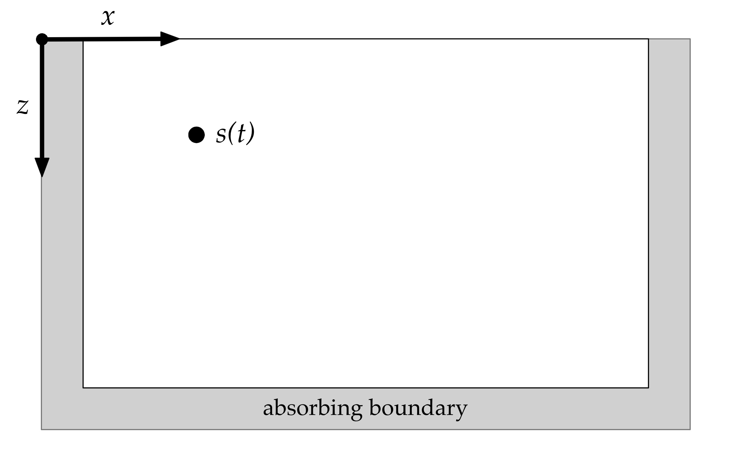
(a)

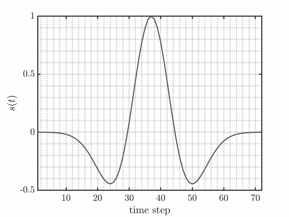
(b)

Figure 1: Domain of interest with absorbing boundary layers (left) and Ricker’s wavelet; $\sigma_{R}=7.5$ (right).

4 Numerical examples

4.1 Uniform velocity field (Homogeneous medium)

We first present a basic example of simulation of wave propagation in a homogeneous medium to verify RBF-FD and FDM implementations. Since RBF-FD can mimic FDM when the same grid layout is used, we can compare the solution obtained with RBF-FD and FDM, to analyse both methods and also compare the effect of ABCs.

We define the problem on a square domain with dimensions $(500\,\mathrm{m},500\,\mathrm{m})$. The wave velocity is set to $v=3000\,\mathrm{m/s}$ and is kept constant, implying a constant nodal spacing of $h=1.1\,\mathrm{m}$ which gives $N=248572$ nodes. The source of the Ricker’s wavelet is defined to be $(x_{s},z_{s})=(150\,\mathrm{m},150\,\mathrm{m})$, and the shape parameter used was $\sigma_{R}=0.00147\,\mathrm{s^{-1}}$.

A grid with a comparable number of nodes $N_{\text{FDM}}=250000$ (with nodal spacing of $h_{\text{FDM}}=1\,\mathrm{m}$) was used in FDM simulation.

Stencils for RBF-FD were computed as $n=7$ closest nodes (including the node itself). and shape parameter for Gaussians is $\sigma_{B}=70\,\mathrm{m}$.

We used a small enough time step of $dt=0.000098\,\mathrm{s}$ to obtain a stable solution. The time step was the same in both methods.

To compare the solutions, they were re-interpolated to the same grid using linear interpolation. The pressure fields and pressure differences shown are in units of $\mathrm{N/m^{2}}$.

Figure 2 shows the wavefield at two different times. The initial shock propagates in a circular shape until it makes contact with the boundary of the domain, after which is is completely reflected at the top, but partially absorbed on the left. The lower two plots illustrate the state after the reflections, where the effect of absorbing boundary conditions can be observed.

In general, RBF-FD and FDM solution agree well in scope of error presented in Figure 3. However, in first three plots of Figure 3 one can observe periodic difference between both solutions on the wave circle. To analyse this phenomenon a plot of the wave field on the circle centred at the origin of the source is presented in Figure 4. It would be expected that the displacement fields are constant on this circumference, as the wave is propagating symmetrically. However, as can be observed in the right plot in Figure 4, FDM method displays significant discrepancies from the expected symmetry. While RBF-FD also doesn’t provide perfect rotational symmetry, the discrepancies are noticeably smaller. This difference between methods might be explained by the larger number of support nodes and more symmetric placement employed by RBF-FD method in comparison to FDM.

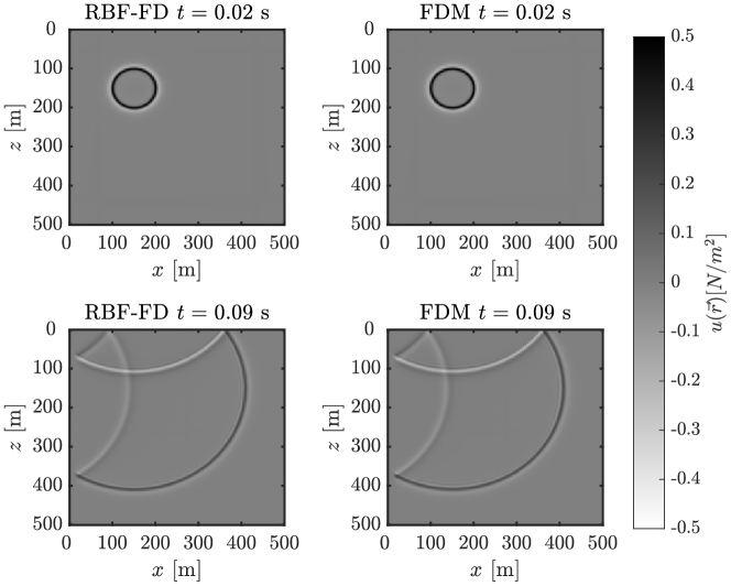
Figure 2: Snapshots of the solution obtained by RBF-FD and FDM method.

The peak value at time $t=70\,\mathrm{ms}$ with respect to the number of nodes is for both methods presented in Figure 5, where it can be seen that both methods converge to the same value.

In geophysics there is special significance to the values of the wavefield at the top boundary - at Earth surface, which is represented with seismogram, i.e. the time evolution of the wavefield values at the top boundary. In the Figure 6 the $x$ axis corresponds to the horizontal spatial dimension, while $y$ axis represents the temporal dimension.

In summary, as expected, in this simple case both method produce comparable and convergent solutions.

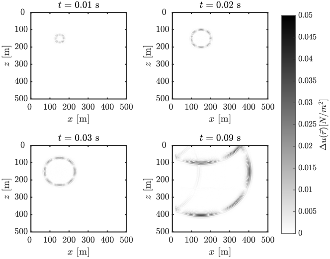
Figure 3: Absolute difference between RBF-FD and 5 point FDM at time four points in time.

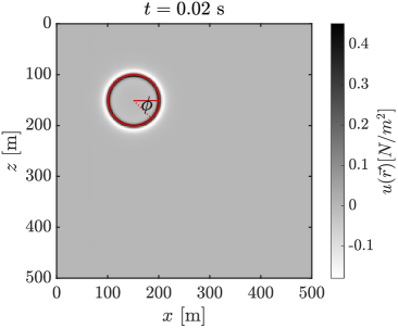
(a) Circle in which wavefield is interpolated.

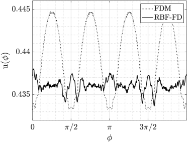
(b) Wavefield interpolated in the circle.

Figure 4: Symmetry of the RBF-FD and FDM solutions.

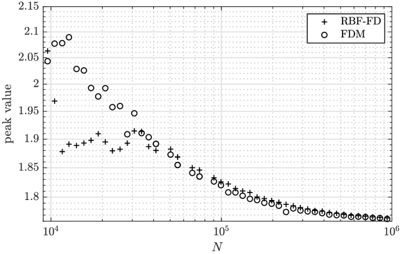
Figure 5: Peak value at $t=0.03\,\mathrm{s}$ with respect to the number of nodes.

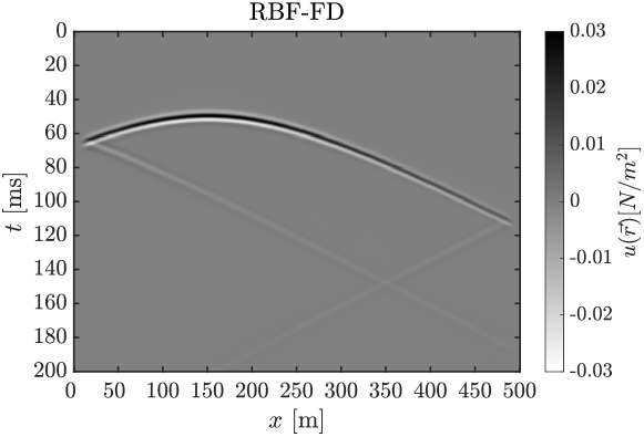
Figure 6: Seismogram obtained with the RBF-FD.

4.2 Two-layer velocity model

In next step we consider a two-layer velocity model. The difference in velocities between layers suggest different distance between nodes as change of velocity causes the wavelength to change. To evade numerical artifacts it is important that an sufficient amount of nodes (10 – 20) is present per wavelength Geiger and Daley [2003], Alford et al. [1974]. Using the RBF-FD meshless method, there aren’t any restrictions on node placement, which gives it an advantage over conventional methods. Consequently variable node density in relationship to the velocity field is easily implemented.

In Figure 7 the $z$ cross-section velocity profile and corresponding RBF-FD nodes are presented. The jump in velocity happens at depth of $80\,\mathrm{m}$. It can be observed that the jump in inter-nodal distances doesn’t directly follow the jump in velocity. The jump happens at depth of $150\,\mathrm{m}$. The inter-nodal distance function $h(z)$ is made continuous by application of a moving average over the step function

$$h(z)=\text{moving average}(0.737843\,\mathrm{m}+H(z-150\,\mathrm{m})\text{ }0.737847\,\mathrm{m}),$$ (14)

where $H$ is the Heaviside step function. The displacement of the jump in node density is a necessary compromise which will be discussed in more detail with the presentation of the results. Dimensions of the domain are $(500\,\mathrm{m},500\,\mathrm{m})$. For RBF-FD method time step is set to $dt=0.000058\,\mathrm{s}$ and for FDM method it is set to $dt=0.000167\,\mathrm{s}$. The source is located at $(x_{s},z_{s})=(250\,\mathrm{m},200\,\mathrm{m})$, and parameter $\sigma_{R}=0.00106\,\mathrm{s^{-1}}$ was used for the Ricker’s wavelet. As stated previously parameter $\epsilon=4\,\mathrm{m}$ was used.

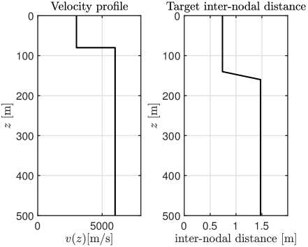
(a)

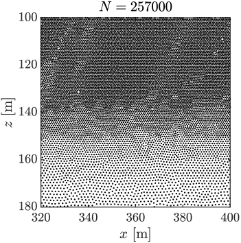
(b)

Figure 7: $z$ cross-section velocity profile (left), $z$ cross-section inter-nodal distance function (center) and snapshot of node placement (right).

Snapshots of the wavefield are presented at 4 different times in Figure 8. Again we observe the reduced reflections from the boundary. A new phenomenon present in this case is the partial reflection at $y=250\,\mathrm{m}$. This is most clearly visible at time $t=0.03\,\mathrm{s}$, where this is the only reflection resent in addition to the original wave propagating from the source. Decreasing of wavelength can be observed as well.

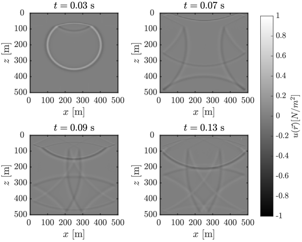
Figure 8: RBF-FD solution snapshots.

The results from RBF-FD are compared to those from FDM in Figure 9. Both methods are tested on discretization with approximately $250000$ nodes, however RBF-FD method distributes nodes as described at the beginning of this subsection in contrast to homogeneous grid used by FDM.

In Figure 9 artificial ripples are present on snapshot of FDM solution, which do not develop when the RBF-FD solution is employed.

Such errors are caused by insufficient node density. Using RBF-FD this problem was avoided, by increasing the density in upper region while simultaneously decreasing the density in lower region, which does not reduce the accuracy as much since the wavelength in the lower region is larger.

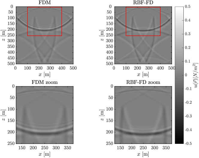
Figure 9: Snapshot at time 0.13s.

As stated before, the step in velocity and the decrease in node density do not align exactly. This necessitated by the fact that sudden jumps in nodal density cause new numerical errors and the fact that nodal density must be sufficiently high everywhere on the domain. If just a moving average of the velocity field would be used as the basis for target inter-node distance function, the second condition would not be met in narrow region on top of the point of velocity step. For best results it proved necessary to delay the jump in node density in comparison to point of jump in velocity field.

In addition to slightly increasing the amount of nodes necessary, another downside is introduced. If the node density used with RBF-FD directly followed the velocity field, the solution would actually be more stable than one provided by FDM. This can be understood by looking at the stability criterion for FDM:

$$dt\varpropto\frac{dx}{v}.$$ (15)

When using FDM the only change in comparison to case with constant velocity is the increase of the velocity in the lower half of the domain. Flowing the criterion, this results in smaller required time-step for all of the simulation. When RBF-FD is used depending on nodal distribution two cases are possible:

• If the nodal density follows the velocity field directly, meaning $dx\propto v$ , the velocity dependance of the criterion cancels out. This means that areas of high velocity do not dictate the use of shorter time steps in simulation.

• In case where the density field does not follow the velocity field directly, we lose the stability advantage. In the narrow area below the point of velocity step, the node density is unchanged while the velocity increases, this results in same necessity for decrease in time step. The time step actually needs to be even smaller than one required by FDM, as $dx$ in the dense region is smaller than one used by FDM, which reduces time step further as $dt\propto dx$ follows from stability criterion.

All of the discussed assumes the stability criterion for FDM is at least to a factor also valid for RBF-FD. The need for a lower time-step might be a cause for concern, however if one would want similar performance to one achieved using RBF-FD, FDM with grid of higher density would be necessary. Not only would this drastically increase the number of computational nodes, the time-step would also have to match the smaller one used by RBF-FD, as the $dx$ in criterion would now be the same for both methods.

While the difference was already very clear in Figure 9, cross-section view provides even more detailed picture. We look at the cross-section at $x=250\,\mathrm{m}$ in Figure 10. Snapshot is provided at time $t=67\,\mathrm{ms}$.

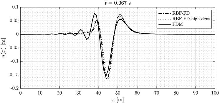
Figure 10: Cross-section.

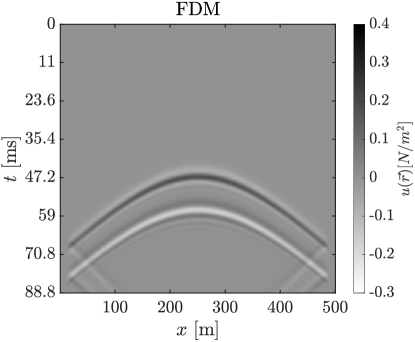
(a)

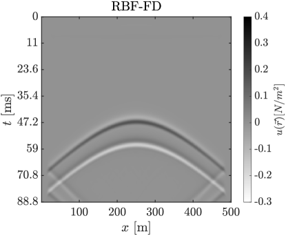
(b)

Figure 11: Seismogram two-layer model.

The RBF-FD solution displayed here always provided at least 11 nodes per characteristic distance of the wave. For reference Another RBF-FD solution is added, where the density is higher, namely at least 15 nodes per characteristic distance.

To conclude the analysis of this numerical example, seismograms are provided for both methods in Figure 11. Again, we can make similar observations about improved accuracy of RBF-FD method in this case.

4.3 Marmousi velocity model

For the last numerical test we look at a more complicated example of Marmousi velocity model Versteeg [1994], displayed in the left of Figure 12. Similarly as in section on Numerical test 2, the node density can be related linearly to the velocity field, however in this case without displacing and smoothing, as we will ensure enough nodes in high-velocity area for stable simulation. Since the data points of the velocity model do not generally align with the positions of computational nodes, Sheppard’s scattered data interpolation is used to determine the density at the required positions.

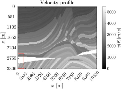
(a)

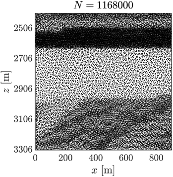
(b)

Figure 12: Velocity profile (left) and node placement (right).

On the right side of Figure 12 a zoomed view of the node placement is displayed. This section is marked with red rectangle on the velocity model. In this test the size of the domain is $(10400\,\mathrm{m},3306\,\mathrm{m})$, the time step is set to $dt=0.00087\,\mathrm{s}$ and the source is positioned at $(5200\,\mathrm{m},330.6\,\mathrm{m})$ The wavefield snap-shot at different time-intervals have been shown in Figure 13.

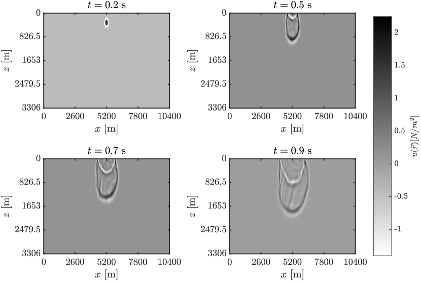
Figure 13: RBF-FD solution snapshots for the Marmousi velocity model.

We can observe the distortion of the primary wave and its reflections caused by the velocity field. The solution is also free of any obvious numerical artifacts.

We provide the seismogram for this example in Figure 14. We can again observe the secondary waves caused by subsurface reflations.

In conjunction with results from previous two cases we can conclude RBF-FD is a viable alternative to conventional methods, such as FDM. It can be applied to cases with arbitrarily complex velocity fields and can reduce numerical artifacts without drastically increasing computational intensity.

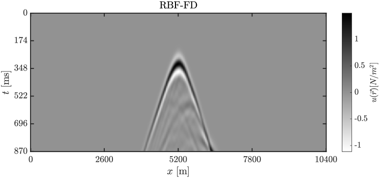
Figure 14: Marmousi seismogram.

4.4 Irregular domain shape: Canadian Foothill

To demonstrate performance of presented RBF-FD based solution procedure on irregular domains, the Canadian Foothill model is addressed Gray and Marfurt [1995]. The domain is enclosed inside a rectangle of dimensions $25000\,\mathrm{m}$ times $10000\,\mathrm{m}$ as presented on Figure 15. Sea level is at the $2000\,\mathrm{m}$ mark. The original velocity profile of the model has resolution of $1668$ times $1000$ with data points spaced at $15\,\mathrm{m}$ horizontally and $10\,\mathrm{m}$ vertically.

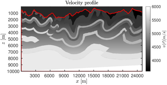
Figure 15: Velocity profile for Canadian Foothill case. Shape of the domain is marked with red line.

The case was set up with a point like source at locations ($12500\,\mathrm{m}$, $2500\,\mathrm{m}$). RBF-FD method was used with time step $dt=0.001\,\mathrm{s}$ on $205964$ scattered nodes positioned with Slak and Kosec [2019c](16).

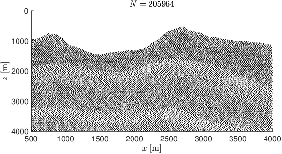
Figure 16: Distribution of nodes, for better visibility only a upper left of the domain is displayed.

First, we solved a simplified model with constant velocity profile $v=4500\,\mathrm{m}$ that is presented in Figure 18. In next step, we included also Canadian Foothill velocity profile, results are presented in Figure 18.

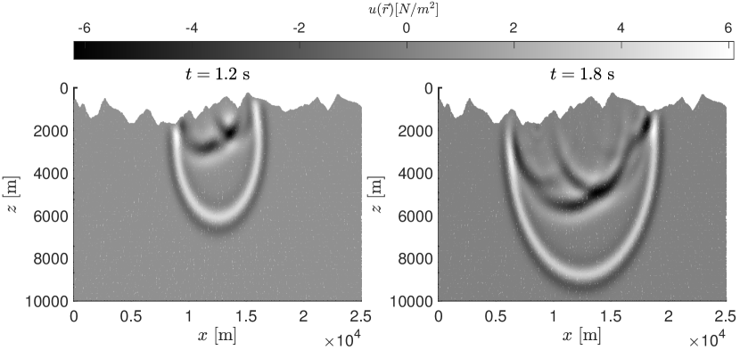
Figure 17: RBF-FD solution snapshot for constant velocity profile $v=4500\,\mathrm{\frac{m}{s}}$.

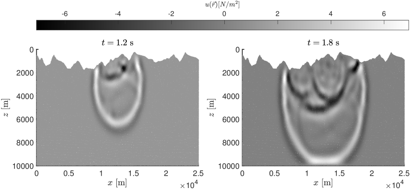
Figure 18: RBF-FD solution snapshot for Canadian Foothill velocity profile.

5 Conclusions

We have investigated a local strong-form meshless method RBF-FD for numerical solution of 2D time-domain acoustic wave equation in heterogeneous media. The numerical tests performed here have twofold importance: (a) It is one more-step towards the robustness of the current understanding of the RBF-FD by exploring the acoustic wave propagation problem, and (b) the RBF-FD has the potential of being used in large-scale seismic modeling and inversion applications. Followings are some conclusions we draw from the present study:

1. RBF-FD has the advantage of working with node-distribution, which are adaptive to the given velocity-variations. This is a clear advantage over conventional finite difference method. Moreover, RBF-FD save the effort through bypassing the steps of mesh-generation and preserving its shape trough out the time-iteration, which is an advantage over finite-element type methods.

2. Since the stability-criterion in the RBF-FD method can also be adaptive to the velocity model, unlike in standard FD method, RBF-FD need not to use the maximum velocity and consequently over-sampled nodes in some parts of the domain. This lowers the total number of required nodes for highly-complicated velocity models.

3. Although RBF-FD can theoretically deal with highly-non uniform node-distributions, the non-uniformity introduces numerical dispersion. However, since this error is mostly near the source, its contribution to the final observation is not as noticeable as the corresponding undersampled FD method.

4. This manuscript provides the first high-performance (C++) open-source repository for meshfree seismic modeling. We believe the source-codes of the present paper will help readers to have a better understanding of state-of-the art implementation of RBF-FD and promote further improvement in the field with minimal development efforts.

Author’s Contribution

Gregor Kosec and Jure Slak prepared the approximation engines used for numerical solution of the considered problem Jure M. Berljavac, and Pankaj K Mishra prepared numerical solution procedure and analysed results. All authors equally contributed in preparation of the manuscript.

Computer Code Availability

The computer codes and instruction to reproduce the results in this paper are freely available at https://gitlab.com/e62Lab/2019_p_wavepropagation_code .

References

- Alford et al. [1974] R. M. Alford, K. R. Kelly, and D. Mt Boore. Accuracy of finite-difference modeling of the acoustic wave equation. Geophysics, 39(6):834–842, 1974. doi: 10.1190/1.1441689.
- Kelly et al. [1976] K. R. Kelly, R. W. Ward, Sven Treitel, and R. M. Alford. Synthetic seismograms: A finite-difference approach. Geophysics, 41(1):2–27, 1976. doi: 10.1190/1.1440605.
- Tarantola [1984] Albert Tarantola. Inversion of seismic reflection data in the acoustic approximation. Geophysics, 49(8):1259–1266, 1984. doi: 10.1190/1.1441754.
- Dablain [1986] M. A. Dablain. The application of high-order differencing to the scalar wave equation. Geophysics, 51(1):54–66, 1986. doi: 10.1190/1.1442040.
- Williamson and Pratt [1995] Paul R. Williamson and R. Gerhard Pratt. A critical review of acoustic wave modeling procedures in 2.5 dimensions. Geophysics, 60(2):591–595, 1995. doi: 10.1190/1.1443798.
- Jo et al. [1996] Churl-Hyun Jo, Changsoo Shin, and Jung Hee Suh. An optimal 9-point, finite-difference, frequency-space, 2-D scalar wave extrapolator. Geophysics, 61(2):529–537, 1996. doi: 10.1190/1.1443979.
- Carcione et al. [2002] Jose M. Carcione, Gérard C. Herman, and A. P. E. Ten Kroode. Seismic modeling. Geophysics, 67(4):1304–1325, 2002. doi: 10.1190/1.1500393.
- Geiger and Daley [2003] H. D. Geiger and P. F. Daley. Finite difference modelling of the full acoustic wave equation in Matlab. resreport 15, CREWES Research Report, 2003. URL https://www.crewes.org/ForOurSponsors/ResearchReports/2003/2003-18.pdf.
- Du and Bancroft [2004] Xiang Du and John C. Bancroft. 2-D wave equation modeling and migration by a new finite difference scheme based on the Galerkin method. In SEG Technical Program Expanded Abstracts 2004, pages 1107–1110. Society of Exploration Geophysicists, 2004. doi: 10.1190/1.1851077.
- Liu and Sen [2011] Yang Liu and Mrinal K. Sen. Finite-difference modeling with adaptive variable-length spatial operators. Geophysics, 76(4):T79–T89, 2011. doi: 10.1190/1.3587223.
- Virieux et al. [2012] Jean Virieux, Vincent Etienne, Victor Cruz-Atienza, Romain Brossier, Emmanuel Chaljub, Olivier Coutant, Stphane Garambois, Diego Mercerat, Vincent Prieux, Stphane Operto, Alessandra Ribodetti, and Josu Tago. Modelling seismic wave propagation for geophysical imaging. In Seismic Waves - Research and Analysis. InTech, jan 2012. doi: 10.5772/30219.
- Wang et al. [2016] Enjiang Wang, Yang Liu, and Mrinal K. Sen. Effective finite-difference modelling methods with 2-D acoustic wave equation using a combination of cross and rhombus stencils. Geophysical Journal International, 206(3):1933–1958, 2016. doi: 10.1093/gji/ggw250.
- Wang et al. [2018] Enjiang Wang, Jing Ba, and Yang Liu. Time-space-domain implicit finite-difference methods for modeling acoustic wave equations. Geophysics, 83(4):T175–T193, 2018. doi: 10.1190/geo2017-0546.1.
- Wang et al. [2019] Ning Wang, Hui Zhou, Hanming Chen, Yufeng Wang, Jinwei Fang, Pengyuan Sun, Jianlei Zhang, and Yukun Tian. An optimized parallelized sgfd modeling scheme for 3d seismic wave propagation. Computers & Geosciences, 131:102–111, 2019.
- Cai et al. [2018] Xiaohui Cai, Yang Liu, and Zhiming Ren. Acoustic reverse-time migration using gpu card and posix thread based on the adaptive optimal finite-difference scheme and the hybrid absorbing boundary condition. Computers & Geosciences, 115:42–55, 2018.
- Marfurt [1984] Kurt J. Marfurt. Accuracy of finite-difference and finite-element modeling of the scalar and elastic wave equations. Geophysics, 49(5):533–549, 1984. doi: 10.1190/1.1441689.
- Emmerich and Korn [1987] Helga Emmerich and Michael Korn. Incorporation of attenuation into time-domain computations of seismic wave fields. Geophysics, 52(9):1252–1264, 1987. doi: 10.1190/1.1442386.
- De Basabe and Sen [2007] Jonás D. De Basabe and Mrinal K. Sen. Grid dispersion and stability criteria of some common finite-element methods for acoustic and elastic wave equations. Geophysics, 72(6):T81–T95, 2007. doi: 10.1190/1.2785046.
- Ham and Bathe [2012] Seounghyun Ham and Klaus-Jürgen Bathe. A finite element method enriched for wave propagation problems. Computers & structures, 94:1–12, 2012. doi: 10.1016/j.compstruc.2012.01.001.
- Seriani and Priolo [1994] Géza Seriani and Enrico Priolo. Spectral element method for acoustic wave simulation in heterogeneous media. Finite elements in analysis and design, 16(3-4):337–348, 1994. doi: 10.1016/0168-874X(94)90076-0.
- Seriani and Oliveira [2007] Géza Seriani and Saulo P. Oliveira. Optimal blended spectral-element operators for acoustic wave modeling. Geophysics, 72(5):SM95–SM106, 2007. doi: 10.1190/1.2750715.
- Shukla et al. [2019] Khemraj Shukla, José M Carcione, Reynam C Pestana, Priyank Jaiswal, and Turgut Özdenvar. Modeling the wave propagation in viscoacoustic media: An efficient spectral approach in time and space domain. Computers & Geosciences, 126:31–40, 2019.
- Malovichko et al. [2018] Mikail Malovichko, Nikolay Khokhlov, Nikolay Yavich, and Mikhail Zhdanov. Acoustic 3d modeling by the method of integral equations. Computers & Geosciences, 111:223–234, 2018.
- Jastram and Behle [1992] Cord Jastram and Alfred Behle. Acoustic modelling on a grid of vertically varying spacing. Geophysical prospecting, 40(2):157–169, 1992. doi: 10.1111/j.1365-2478.1992.tb00369.x.
- Hayashi et al. [2001] Koichi Hayashi, Daniel R. Burns, and M. Nafi Toksöz. Discontinuous-grid finite-difference seismic modeling including surface topography. Bulletin of the Seismological Society of America, 91(6):1750–1764, 2001. doi: 10.1785/0120000024.
- Kang and Baag [2004] Tae-Seob Kang and Chang-Eob Baag. An efficient finite-difference method for simulating 3D seismic response of localized basin structures. Bulletin of the Seismological Society of America, 94(5):1690–1705, 2004. doi: 10.1785/012004016.
- Kristek et al. [2010] Jozef Kristek, Peter Moczo, and Martin Galis. Stable discontinuous staggered grid in the finite-difference modelling of seismic motion. Geophysical Journal International, 183(3):1401–1407, 2010. doi: 10.1111/j.1365-246x.2010.04775.x.
- Chu and Stoffa [2012] Chunlei Chu and Paul L. Stoffa. Nonuniform grid implicit spatial finite difference method for acoustic wave modeling in tilted transversely isotropic media. Journal of Applied Geophysics, 76:44–49, 2012. doi: 10.1016/j.jappgeo.2011.09.027.
- Fornberg [1988] Bengt Fornberg. Generation of finite difference formulas on arbitrarily spaced grids. Mathematics of computation, 51(184):699–706, 1988. doi: 10.1090/s0025-5718-1988-0935077-0.
- Slak and Kosec [2019a] Jure Slak and Gregor Kosec. Adaptive radial basis function-generated finite differences method for contact problems. International Journal for Numerical Methods in Engineering, 119(7):661–686, August 2019a. doi: 10.1002/nme.6067.
- Tolstykh and Shirobokov [2003] A. I. Tolstykh and D. A. Shirobokov. On using radial basis functions in a “finite difference mode” with applications to elasticity problems. Computational Mechanics, 33(1):68–79, 2003. doi: 10.1007/s00466-003-0501-9.
- Fornberg and Flyer [2015] Bengt Fornberg and Natasha Flyer. Solving PDEs with radial basis functions. Acta Numerica, 24:215–258, May 2015. ISSN 0962-4929, 1474-0508. doi: 10.1017/S0962492914000130.
- Bayona et al. [2017] Victor Bayona, Natasha Flyer, Bengt Fornberg, and Gregory A. Barnett. On the role of polynomials in RBF-FD approximations: II. Numerical solution of elliptic PDEs. Journal of Computational Physics, 332:257–273, 2017. doi: 10.1016/j.jcp.2016.12.008.
- Slak and Kosec [2019b] Jure Slak and Gregor Kosec. Refined meshless local strong form solution of Cauchy–Navier equation on an irregular domain. Engineering Analysis with Boundary Elements, 100:3–13, mar 2019b. ISSN 0955-7997. doi: 10.1016/j.enganabound.2018.01.001.
- Mishra et al. [2019] Pankaj K Mishra, Gregory E Fasshauer, Mrinal K Sen, and Leevan Ling. A stabilized radial basis-finite difference (RBF-FD) method with hybrid kernels. Computers & Mathematics with Applications, 77(9):2354–2368, 2019.
- Slak and Kosec [2019c] Jure Slak and Gregor Kosec. On generation of node distributions for meshless PDE discretizations. SIAM Journal on Scientific Computing, 41(5):A3202–A3229, October 2019c. doi: 10.1137/18M1231456.
- Jia et al. [2005] Xiaofeng Jia, Tianyue Hu, and Runqiu Wang. A meshless method for acoustic and elastic modeling. Applied Geophysics, 2(1):1–6, 2005. doi: 10.1007/s11770-005-0001-0.
- Hahn and Negrut [2009] Philipp Hahn and Dan Negrut. On the use of meshless methods in acoustic simulations. In ASME 2009 International Mechanical Engineering Congress and Exposition, pages 185–199. American Society of Mechanical Engineers, 2009. doi: 10.1115/imece2009-11351.
- Zhang et al. [2016] Y. O. Zhang, T. Zhang, H. Ouyang, and T. Y. Li. Efficient SPH simulation of time-domain acoustic wave propagation. Engineering Analysis with Boundary Elements, 62:112–122, 2016. doi: 10.1190/geo2016-0464.1.
- Takekawa et al. [2015] Junichi Takekawa, Hitoshi Mikada, and Naoto Imamura. A mesh-free method with arbitrary-order accuracy for acoustic wave propagation. Computers & Geosciences, 78:15–25, 2015. doi: 10.1016/j.cageo.2015.02.006.
- Takekawa and Mikada [2016] Junichi Takekawa and Hitoshi Mikada. A mesh-free finite-difference method for frequency-domain viscoacoustic wave equation. In SEG Technical Program Expanded Abstracts 2016, pages 3841–3845. Society of Exploration Geophysicists, 2016. doi: 10.1190/segam2016-13457674.1.
- Liu et al. [2017] Xin Liu, Bei Li, and Yang Liu. A perfectly matched layer boundary condition for acoustic-wave simulation in mesh-free discretization using frequency-domain radial-basis-function-generated finite difference. In SEG Technical Program Expanded Abstracts 2017, pages 4231–4235. Society of Exploration Geophysicists, 2017. doi: 10.1190/segam2017-17661221.1.
- Mishra et al. [2017] Pankaj Mishra, Sankar Nath, Gregory Fasshauer, and Mrinal Sen. Frequency-domain meshless solver for acoustic wave equation using a stable radial basis-finite difference (RBF-FD) algorithm with hybrid kernels. In SEG Technical Program Expanded Abstracts 2017, pages 4022–4027. Society of Exploration Geophysicists, 2017. doi: 10.1190/segam2017-17494511.1.
- Takekawa and Mikada [2018] Junichi Takekawa and Hitoshi Mikada. A mesh-free finite-difference method for elastic wave propagation in the frequency-domain. Computers & Geosciences, 118:65–78, 2018.
- Li et al. [2017] B. Li, Y. Liu, M. K. Sen, and Z. Ren. Time-space-domain mesh-free finite difference based on least squares for 2D acoustic-wave modeling. Geophysics, 82(4):T143–T157, 2017. doi: 10.1190/geo2016-0464.1.
- Slak and Kosec [2019d] Jure Slak and Gregor Kosec. Medusa: A C++ library for solving pdes using strong form mesh-free methods, 2019d. URL http://e6.ijs.si/medusa/.
- Cerjan et al. [1985] Charles Cerjan, Dan Kosloff, Ronnie Kosloff, and Moshe Reshef. A nonreflecting boundary condition for discrete acoustic and elastic wave equations. Geophysics, 50(4):705–708, 1985. doi: 10.1190/1.1441945.
- Versteeg [1994] Roelof Versteeg. The Marmousi experience: Velocity model determination on a synthetic complex data set. The Leading Edge, 13(9):927–936, sep 1994. doi: 10.1190/1.1437051.
- Gray and Marfurt [1995] Samuek Gray and Kurt J Marfurt. Migration from topography: Improving the near-surface image. Canadian Journal of Exploration Geophysics, 1995.