On Output Feedback Stabilization of Time-Varying Decomposable Systems with Switching Topology and Delay^⋆

Abstract

This paper presents a new method for dynamic output feedback stabilizing controller design for decomposable systems with switching topology and delay. Our approach consists of two steps. In the first step, we model the decomposable systems with switching topology as equivalent LPV systems with a piecewise constant parameter. In the second step, we design stabilizing output feedbacks for these LPV systems in the presence of a time-varying output delay using a trajectory-based stability analysis approach. We do not impose any constraint on the delay derivative. Finally, we illustrate our approach by applying it to the consensus problem of non-holonomic agents.

1 Introduction

A distributed system is a swarm of subsystems that are connected physically or through communication protocols with each subsystem having information about the interconnection topology. Such systems emerge in many application domains such as vehicle platooning (Jovanovic and Bamieh, 2005), multi-UAV formation flight (Betser et al., 2005), satellite formation (Mesbahi and Hadaegh, 2001; Carpenter, 2000), paper machine problem (Stewart et al., 2003), and large segmented telescopes (Jiang et al., 2006). Motivated by these real-world applications, many researchers have studied various problems related to distributed systems such as consensus problem, flocking problem, and formation problem; see Li and Duan (2014). The decomposable system (or identical dynamically decoupled system), on the other hand, is a special class of distributed systems with identical subsystems interacting with each other. Tools from the algebraic graph theory, such as Laplacian matrices, or graph-adjacency matrices (known as pattern matrices) are used to represent the interactions among the subsystems of a decomposable system; see Borrelli and Keviczky (2008). A general overview of these systems, and their applications are provided in Massioni and Verhaegen (2009), Ghadami and Shafai (2013), and Eichler et al. (2014).

Since time delay may affect the performance of a distributed network in practice due to non-ideal signal transmission, the study of distributed systems with a delay is strongly motivated. Therefore, many efforts have been made in the literature to tackle the issues of stability and performance degradation caused by communication or network delay in distributed systems; see Atay (2013), Ghaedsharaf et al. (2016), Olfati-Saber and Murray (2004), Papachristodoulou et al. (2010), Qiao and Sipahi (2016), Seuret et al. (2008), and Sun and Wang (2009). Apart from time delays, another interesting phenomenon in distributed systems is switching topology, where the interconnection links may change over time due to various reasons. For example, communicating mobile agents may lose an existing connection due to the presence of an obstacle. On the other hand, a new connection may be established between the agents when they come close to each other in an effective range of detection.

In this paper, we provide a new method for dynamic output feedback stabilization of time-varying decomposable systems with switching topology and delay. Our technique involves two steps. First, we model a decomposable system with switching topology as an equivalent LPV system with a piecewise constant parameter. Then, we use a trajectory-based approach to design output feedback controllers, ensuring the stability of this class of LPV systems in the presence of a time-varying pointwise output delay. Both of these steps are important for their own sakes and can be considered as two seperate contributions of this paper. Motivated by the serious obstacle presented by the search for suitable Lyapunov functionals for switched and LPV systems with delay, we employ a trajectory-based stability result, proposed in Ahmed et al. (2018). We allow the delay to be a piecewise continuous function of time, and we do not impose any constraint on the delay derivative, which makes it possible to apply our approach to systems where the delay cannot be approximated by a differentiable delay with a bounded first derivative. Typical examples of this phenomenon include data flow across a communication network and delay resulting from sampling. While Ahmed et al. (2018) considers switched systems with countable modes, here we extend their results to switched systems with an uncountable number of modes. Stability analysis and control of LPV systems with piecewise constant parameters is also presented in Briat (2015b). However, there are two key differences between Briat (2015b) and the present work, (i) no delay is present in Briat (2015b), (ii) we study output feedback control, whereas state feedback control is discussed in Briat (2015b). Our work can be regarded as an extension of Zakwan and Ahmed (2020), offering new advantages, because (i) we use a trajectory-based approach for stability analysis which circumvents the serious obstacle presented by the search for appropriate Lyapunov functionals, (ii) we do not impose any constraint on the upper bound of the delay derivative.

The paper unfolds as follows. Section 2 presents modeling of decomposable systems with switching topology as equivalent LPV systems with a piecewise constant parameter. The output feedback stabilizing controller design appears in Section 3. The application of our results to multi-agent nonholonomic systems is presented in Section 4, and Section 5 presents concluding remarks and some future perspectives.

The notation will be simplified whenever no confusion can arise from the context. The identity matrix of appropriate dimension and the Kronecker product are denoted by $I$ and $\otimes$, respectively. The set of real numbers and the set of nonnegative real numbers are denoted by $\mathbb{R}$ and $\mathbb{R}_{\geq 0}$, respectively. The set of positive integers and the set of whole numbers are denoted by $\mathbb{N}$ and $\mathbb{N}_{0}:=\mathbb{N}\cup\{0\}$, respectively. The usual Euclidean norm of vectors, and the induced norm of matrices, are denoted by $|\cdot|$. Given any constant $\tau>0$, we let $C([-\tau,0],\mathbb{R}^{n})$ denote the set of all continuous $\mathbb{R}^{n}$-valued functions that are defined on $[-\tau,0]$. We abbreviate this set as $C_{\rm in}$, and call it the set of all initial functions. Also, for any continuous function $x:[-\tau,\infty)\rightarrow\mathbb{R}^{n}$ and all $t\geq 0$, we define $x_{t}$ by $x_{t}(\theta)=x(t+\theta)$ for all $\theta\in[-\tau,0]$, i.e., $x_{t}\in C_{\rm in}$ is the translation operator. A vector or a matrix is nonnegative (resp. positive) if all of its entries are nonnegative (resp. positive). We write $M\succ 0$ (resp. $M\preceq 0$) to indicate that $M$ is a symmetric positive definite (resp. negative semi-definite) matrix. For two vectors $V=(v_{1}...v_{n})^{\top}$ and $U=(u_{1}...u_{n})^{\top}$, we write $V\leq U$ to indicate that for all $i\in\{1,...,n\}$, $v_{i}\leq u_{i}$.

2 LPV Modeling of Decomposable Systems with Switching Topology

Let us consider an $Nn$-th order interconnected linear time-varying system

$$\begin{array}[]{rcl}\dot{x}(t)&=&{A(t)}x(t)+{B(t)}u(t)\\[2.84526pt] y(t)&=&{C(t)}x(t-\tau(t))\end{array}$$ (1)

with $x\in\mathbb{R}^{Nn}$, $u\in\mathbb{R}^{Nd_{u}}$, $y\in\mathbb{R}^{Nd_{y}}$, $x_{t}\in C_{\rm in}$, and for all $t\geq 0$, $\tau(t)\in[0,\overline{\tau}]$ with $\overline{\tau}>0$.

We introduce a range dwell-time condition, i.e., a sequence of real numbers $t_{k}$ such that there are two positive constants $\underline{\delta}$ and $\overline{\delta}$ such that $t_{0}=0$ and for all $k\in\mathbb{N}_{0}$,

$$t_{k+1}-t_{k}\in[\underline{\delta},\overline{\delta}]\;.$$ (2)

We start by formally defining decomposable matrices, which are of interest in describing the systems considered in this paper.

Definition 1 (Eichler et al., 2014)

A matrix ${M(t)}:\mathbb{R}\rightarrow\mathbb{R}^{Np\times Nq}$ is called decomposable if given a matrix $\mathcal{P}(t):\mathbb{R}\rightarrow\mathbb{R}^{N\times N}$ (pattern matrix), there exist matrices $\bar{M}^{a}$, $\bar{M}^{b}\in\mathbb{R}^{p\times q}$ such that

$$M(t)=I_{N}\otimes\bar{M}^{a}+\mathcal{P}(t)\otimes\bar{M}^{b}$$ (3)

for all $t\geq 0$, where the superscript $a$ represents the decentralized part and superscript $b$ represents the interconnected part. $\hfill\square$

We can now define the class of systems studied in this paper.

Definition 2 (Eichler et al., 2014)

The system (1) is called decomposable if and only if all of its system matrices are decomposable, i.e., can be written as (3) for the same matrix $\mathcal{P}(t)$. $\hfill\square$

We define the pattern matrix $\mathcal{P}(t)$ as a linear convex combination of two symmetric commutable matrices $\mathcal{P}_{1}$ and $\mathcal{P}_{2}$, i.e.,

$$\begin{array}[]{rcl}\mathcal{P}(t)=\sigma(t)\mathcal{P}_{1}+(1-\sigma(t))\mathcal{P}_{2}\;,\end{array}$$ (4)

where $\sigma(t)\in[0,1]$ is a piecewise constant switching signal satisfying the range dwell-time condition (2). Moreover, $\dot{\sigma}(t)=0$ between the jumps and $\sigma(t)$ arbitrarily change its value with a finite jump intensity. Since the symmetric matrices $\mathcal{P}_{1}$ and $\mathcal{P}_{2}$ commute with each other, there exists a unitary matrix $U$ that simultaneously diagonalizes the pair $\mathcal{P}_{1},\mathcal{P}_{2}$ according to (Horn and Johnson, 2012, Theorem 1.3.12). Therefore, we can write (4) as

$$\begin{array}[]{rcl}\Lambda(t)=\sigma(t)\Lambda_{1}+(1-\sigma(t))\Lambda_{2}\;,\end{array}$$

where $\Lambda(t):\mathbb{R}\mapsto\mathbb{R}^{N}$ is a matrix-valued function, $\Lambda_{1}\ \text{and}\ \Lambda_{2}$ are constant block diagonal matrices each of size $N$, and let $\lambda_{1i}$ and $\lambda_{2i}$ denote the $i$-th eigenvalues of the matrices $\mathcal{P}_{1}$ and $\mathcal{P}_{2}$, respectively.

Remark 1

The convex combination given in (4) is not unique, any linear convex combination is admissible, e.g.,

$$\begin{array}[]{rcl}\mathcal{P}(t)={\mathcal{P}_{1}+\mathcal{P}_{2}+\sigma(t)(\mathcal{P}_{2}-\mathcal{P}_{1})\over 2}\;,\end{array}$$

where $\sigma(t)\in[-1,1]$. $\hfill\square$

We provide a theorem that will be substantial in proving the results in the sequel.

Theorem 1

An $Nn$-$th$ order system (1) as described in definition 2 is equivalent to $N$ independent subsystems of order $n$

$$\begin{array}[]{rcl}\dot{\hat{x}}_{i}(t)&=&A^{\dagger}(\nu_{i})\hat{x}_{i}(t)+B^{\dagger}(\nu_{i})\hat{u}_{i}(t)\\[2.84526pt] \hat{y}_{i}(t)&=&C^{\dagger}(\nu_{i})\hat{x}_{i}(t-\tau(t))\quad\text{for}\ i=1,2,...,N\;,\end{array}$$ (5)

where $\hat{x}_{i}\in\mathbb{R}^{n}$, $\hat{u}_{i}\in\mathbb{R}^{d_{u}}$, $\hat{y}_{i}\in\mathbb{R}^{d_{y}}$, and $\nu_{i}(t)=\sigma(t)\lambda_{1i}+(1-\sigma(t))\lambda_{2i}$. Moreover, the matrices $A^{\dagger}(\nu_{i})$, $B^{\dagger}(\nu_{i})$, and $C^{\dagger}(\nu_{i})$ are defined as

$$\begin{array}[]{rcl}A^{\dagger}(\nu_{i})&=&{\bar{A}}^{a}+\nu_{i}{\bar{A}}^{b}\\[2.84526pt] B^{\dagger}(\nu_{i})&=&{\bar{B}}^{a}+\nu_{i}{\bar{B}}^{b}\\[2.84526pt] C^{\dagger}(\nu_{i})&=&{\bar{C}}^{a}+\nu_{i}{\bar{C}}^{b}\;.\end{array}$$ (6)

Remark 2

Interconnected systems in which each subsystem has the same delay, appear in many real-world applications; see Zhou and Lin (2014) for the motivation of this assumption. $\hfill\square$

Let us define the set

$$\mathscr{P}=\left\{\begin{array}[]{ccl}\rho:\mathbb{R}_{\geq 0}\rightarrow P:\rho(t)=p_{k}\in P,\\[2.84526pt] t\in[t_{k},\ t_{k+1}),\ k\in\mathbb{N}_{0}\end{array}\right\}\;,$$

where $P$ is compact and connected.

We now provide a method to model a decomposable system with switching topology as an LPV system with a piecewise constant parameter.

Theorem 2

The system (1) as described in definition 2 is equivalent to an LPV system

$$\begin{array}[]{rcl}\dot{\omega}(t)&=&\mathcal{A}(\rho)\omega(t)+\mathcal{B}(\rho)v(t)\\[2.84526pt] r(t)&=&\mathcal{C}(\rho)\omega(t-\tau(t))\;,\end{array}$$ (7)

where $\omega\in\mathbb{R}^{n}$, $v\in\mathbb{R}^{d_{u}}$, $r\in\mathbb{R}^{d_{y}}$, and the piecewise constant parameter $\rho\in\mathscr{P}$ satisfies the dwell-time condition (2) and takes arbitrary values in the interval $[\min\{\underline{\lambda}_{1},\underline{\lambda}_{2}\},\ \max\{\bar{\lambda}_{1},\bar{\lambda}_{2}\}]$, where $\underline{\lambda}_{j},\ \bar{\lambda}_{j}$ are minimum and maximum eigenvalues of $\mathcal{P}_{j}$ for $j=1,2$, respectively. Moreover, the matrices $\mathcal{A}(\rho),\mathcal{B}(\rho),\text{and}\ \mathcal{C}(\rho)$ are given by

$$\begin{array}[]{rcl}\mathcal{A}(\rho)&=&{\bar{A}}^{a}+\rho{\bar{A}}^{b}\\[2.84526pt] \mathcal{B}(\rho)&=&{\bar{B}}^{a}+\rho{\bar{B}}^{b}\\[2.84526pt] \mathcal{C}(\rho)&=&{\bar{C}}^{a}+\rho{\bar{C}}^{b}\;.\end{array}$$

3 Output Feedback Controller Design

In this section, we present output feedback stabilizing controller design for the LPV system with a piecewise constant parameter given in (7).

We start by introducing an assumption.

Assumption 1

(i) There exist a matrix $\mathcal{K}(\rho)$ for all $\rho\in\mathscr{P}$ and constants $T\geq\bar{\tau}$, $a\in[0,1)$, and $b\geq 0$, such that the solutions of the system

$$\dot{\alpha}(t)=\mathcal{M}(\rho)\alpha(t)+\zeta(t)$$

with $\mathcal{M}(\rho)=\mathcal{A}(\rho)+\mathcal{B}(\rho)\mathcal{K}(\rho)$ and $\zeta$ being a piecewise continuous function, satisfy

$$|\alpha(t)|\leq a|\alpha(t-T)|+b\displaystyle\sup_{\ell\in[t-T,t]}|\zeta(\ell)|$$

for all $t\geq T$.
(ii) There exist a matrix $\mathcal{L}(\rho)$ for all $\rho\in\mathscr{P}$ and constants $T\geq\bar{\tau}$, $c\in[0,1)$, and $d\geq 0$, such that the solutions of the system

$$\dot{\beta}(t)=\mathcal{N}(\rho)\beta(t)+\eta(t)$$

with $\mathcal{N}(\rho)=\mathcal{A}(\rho)+\mathcal{L}(\rho)\mathcal{C}(\rho)$ and $\eta$ being a piecewise continuous function, satisfy

$$|\beta(t)|\leq c|\beta(t-T)|+d\displaystyle\sup_{\ell\in[t-T,t]}|\eta(\ell)|$$

for all $t\geq T$. $\hfill\square$

Remark 3

Assumption 1 pertains to the stabilizability and the detectability of the system (7). See Appendix B below on a method to check Assumption 1. $\hfill\square$

Let

$$\begin{array}[]{l}s_{1}\triangleq\sup_{\rho\in\mathscr{P}}|\mathcal{B}(\rho)\mathcal{K}(\rho)|\\[2.84526pt] s_{2}\triangleq\sup_{\rho\in\mathscr{P}}|\mathcal{L}(\rho)\mathcal{C}(\rho)|\\[2.84526pt] s_{3}\triangleq\sup_{\rho\in\mathscr{P}}|\mathcal{M}(\rho)|\;,\end{array}$$ (8)

then we have the following result:

Theorem 3

Let the system (7) satisfy Assumption 1. If for all $t\geq 0$,

$$\tau(t)\leq\bar{\tau}<\bar{\tau}_{u},$$

where

$$\bar{\tau}_{u}=\frac{(1-a)(1-c)}{ds_{1}s_{2}((1-a)+bs_{3})}\;,$$

then the origin of the feedback system

$$\left\{\begin{array}[]{ccl}\dot{\omega}(t)&=&\mathcal{A}(\rho)\omega(t)+\mathcal{B}(\rho)\mathcal{K}(\rho)\hat{\omega}(t)\\[2.84526pt] \dot{\hat{\omega}}(t)&=&\mathcal{A}(\rho)\hat{\omega}(t)+\mathcal{B}(\rho)\mathcal{K}(\rho)\hat{\omega}(t)\\[2.84526pt] &&+\mathcal{L}(\rho)[\mathcal{C}(\rho)\hat{\omega}(t)-r(t)]\\[4.2679pt] r(t)&=&\mathcal{C}(\rho)\omega(t-\tau(t))\end{array}\right.$$ (9)

is globally uniformly exponentially stable (GUES) for all $\rho\in\mathscr{P}$.

Remark 4

The results of Ahmed et al. (2018) apply only to switched systems with countable modes. Here we extend their results to switched systems with an uncountable number of modes, i.e., parameter-dependent systems with a piecewise constant parameter.

Proof.

Let us define the error as $\tilde{\omega}(t)=\hat{\omega}(t)-\omega(t)$. Then

$$\dot{\tilde{\omega}}(t)=\mathcal{A}(\rho)\tilde{\omega}(t)+\mathcal{L}(\rho)[\mathcal{C}(\rho)\hat{\omega}(t)-\mathcal{C}(\rho)\omega(t-\tau(t))]\;.$$

Using $\mathcal{M}(\rho)=\mathcal{A}(\rho)+\mathcal{B}(\rho)\mathcal{K}(\rho)$ and $\mathcal{N}(\rho)=\mathcal{A}(\rho)+\mathcal{L}(\rho)\mathcal{C}(\rho)$, we have

$$\left\{\begin{array}[]{ccl}\dot{\omega}(t)&=&\mathcal{M}(\rho)\omega(t)+\mathcal{B}(\rho)\mathcal{K}(\rho)\tilde{\omega}(t)\\[2.84526pt] \dot{\tilde{\omega}}(t)&=&\mathcal{N}(\rho)\tilde{\omega}(t)+\mathcal{L}(\rho)\mathcal{C}(\rho)[\omega(t)-\omega(t-\tau(t))]\;.\end{array}\right.$$

From Assumption 1 and the equality

$$\begin{array}[]{l}\omega(\ell)-\omega(\ell-\tau(\ell))\\ =\int_{\ell-\tau(\ell)}^{\ell}[\mathcal{M}(\rho(m))\omega(m)+\mathcal{B}(\rho(m))\mathcal{K}(\rho(m))\tilde{\omega}(m)]dm,\end{array}$$

it follows that for all $t\geq T+\bar{\tau}$,

$$|\omega(t)|\leq a|\omega(t-T)|+b\displaystyle\sup_{\ell\in[t-T,t]}|\mathcal{B}(\rho(\ell))\mathcal{K}(\rho(\ell))\tilde{\omega}(\ell)|$$ (10)

$$\begin{array}[]{l}|\tilde{\omega}(t)|\leq c|\tilde{\omega}(t-T)|+d\displaystyle\sup_{\ell\in[t-T,t]}\left|\vphantom{\int_{\ell-\tau(\ell)}^{\ell}}\mathcal{L}(\rho(\ell))\mathcal{C}(\rho(\ell))\right.\\ \left.\times\int_{\ell-\tau(\ell)}^{\ell}[\mathcal{M}(\rho(m))\omega(m)+\mathcal{B}(\rho(m))\mathcal{K}(\rho(m))\tilde{\omega}(m)]dm\right|\;.\end{array}$$ (11)

Using the constants $s_{1}$, $s_{2}$, and $s_{3}$ defined in (8), we deduce from (10) and (11) that $(\omega(t),\tilde{\omega}(t))$ satisfies:

$$\begin{array}[]{ccl}|\omega(t)|&\leq&a|\omega(t-T)|+bs_{1}\displaystyle\sup_{\ell\in[t-T-\bar{\tau},t]}|\tilde{\omega}(\ell)|\;,\\[11.38109pt] |\tilde{\omega}(t)|&\leq&ds_{2}s_{3}\bar{\tau}\displaystyle\sup_{\ell\in[t-T-\bar{\tau},t]}|\omega(\ell)|\\[11.38109pt] &&+(c+ds_{1}s_{2}\bar{\tau})\displaystyle\sup_{\ell\in[t-T-\bar{\tau},t]}|\tilde{\omega}(\ell)|\;.\end{array}$$

Lemma 2 from Appendix A ensures that the origin of (9) is GUES if

$$\left[\begin{array}[]{cc}a&bs_{1}\\ ds_{2}s_{3}\bar{\tau}&ds_{1}s_{2}\bar{\tau}+c\end{array}\right]$$

is Schur stable, which is equivalent to

$$\begin{array}[]{l}\frac{a+c+ds_{1}s_{2}\bar{\tau}}{2}+\\[8.53581pt] \sqrt{\left(\frac{a+c+ds_{1}s_{2}\bar{\tau}}{2}\right)^{2}-ac-ds_{1}s_{2}\left(a-bs_{3}\right)\bar{\tau}}<1\;,\end{array}$$

from which we derive the condition

$$\bar{\tau}<\frac{(1-a)(1-c)}{ds_{1}s_{2}((1-a)+bs_{3})}\;.$$ (12)

This concludes the proof. $\hfill\blacksquare$ ∎

4 Application to Multi-agent Nonholonomic Systems

In this section, we illustrate our approach by applying it to the consensus problem of multi-agent nonholonomic systems subject to switching topology and communication delay. The dynamics of the multi-agent nonholonomic system is adopted from Gonzalez and Werner (2014).

Consider the multi-agent system comprising of six agents ($N=6$) described by

$$\begin{array}[]{rcl}\dot{x}(t)&=&(I_{N}\otimes\bar{A}_{a}+\mathcal{P}(t)\otimes\bar{A}_{b})x(t)\\[2.84526pt] &&+(I_{N}\otimes\bar{B}_{a})u(t)\\[2.84526pt] y(t)&=&(I_{N}\otimes\bar{C}_{a})x(t-\tau(t))\;,\end{array}$$ (13)

where the system matrices are given by

$$\small\begin{array}[]{lll}\bar{A}_{a}=\left[\begin{matrix}0&1\\ -1&0\end{matrix}\right],\ \bar{A}_{b}=\left[\begin{matrix}0&-0.5\\ 0.5&0\end{matrix}\right]\\[8.53581pt] \bar{B}_{a}=\left[\begin{matrix}1&0\\ 0&0.6\end{matrix}\right],\ \bar{C}_{a}=\left[\begin{matrix}1&0\\ 0&1\end{matrix}\right].\end{array}$$

For the multiagent system (13), the pattern matrix is specified as

$$\begin{array}[]{rcl}\mathcal{P}(t)=\sigma(t)\mathcal{P}_{1}+(1-\sigma(t))\mathcal{P}_{2}\;,\end{array}$$

where $\sigma(t)\in[0,\ 1]$ with $\underline{\delta}=0.1,\ \bar{\delta}=0.5$, and the symmetric commutable matrices $\mathcal{P}_{1}$ and $\mathcal{P}_{2}$ are given by

$$\mathcal{P}_{1}=\left[\begin{matrix}1&-0.5&0&0&0&-0.5\\ -0.5&1&-0.5&0&0&0\\ 0&-0.5&1&-0.5&0&0\\ 0&0&-0.5&1&-0.5&0\\ 0&0&0&-0.5&1&-0.5\\ -0.5&0&0&0&-0.5&1\\ \end{matrix}\right]$$

$$\mathcal{P}_{2}=\left[\begin{matrix}1&-0.25&-0.25&0&-0.25&-0.25\\ -0.25&1&-0.25&-0.25&0&-0.25\\ -0.25&-0.25&1&-0.25&-0.25&0\\ 0&-0.25&-0.25&1&-0.25&-0.25\\ -0.25&0&-0.25&-0.25&1&-0.25\\ -0.25&-0.25&0&-0.25&-0.25&1\\ \end{matrix}\right]\;.$$

For the matrices $\mathcal{P}_{1}$ and $\mathcal{P}_{2}$, we have $\min\{\underline{\lambda}_{1},\ \underline{\lambda}_{2}\}=0$, $\max\{\bar{\lambda}_{1},\ \bar{\lambda}_{2}\}=2$. Therefore, by defining a piecewise constant parameter $\rho\in\mathscr{P}\ \text{that takes values in}\ [0,2]$, and then employing Theorem 2, the decomposable system (13) is equivalent to the LPV system

$$\begin{array}[]{rcl}\dot{\omega}(t)&=&\mathcal{A}(\rho)\omega(t)+\mathcal{B}(\rho)v(t)\\[2.84526pt] r(t)&=&\mathcal{C}(\rho)\omega(t-\tau(t))\;,\end{array}$$

where

$$\begin{array}[]{rcl}\mathcal{A}(\rho)=\bar{A}_{a}+\rho\bar{A}_{b},\ \mathcal{B}(\rho)=\bar{B}_{a},\ \text{and}\ \mathcal{C}(\rho)=\bar{C}_{a}\;.\end{array}$$

We choose the controller gains and observer gains as

$$\small\begin{array}[]{rcl}\bar{K}_{a}&=&\bar{L}_{a}=\vspace{1mm}\left[\begin{matrix}-0.5&0\\ 0&-0.5\end{matrix}\right],\\ \bar{K}_{b}&=&\bar{L}_{b}=\left[\begin{matrix}0.1&0\\ 0&0.1\end{matrix}\right].\end{array}$$

Using Theorem 2, we model the distributed controller $K(t)=I_{N}\otimes\bar{K}_{a}+\mathcal{P}(t)\otimes\bar{K}_{b}$ and the distributed observer $L(t)=I_{N}\otimes\bar{L}_{a}+\mathcal{P}(t)\otimes\bar{L}_{b}$ as $\mathcal{K}(\rho)=\bar{K}_{a}+\rho\bar{K}_{b}$ and $\mathcal{L}(\rho)=\bar{L}_{a}+\rho\bar{L}_{b}$, respectively.

In order to satisfy Assumption 1, we proceed as follows. First, we solve the LMIs (16), (17), and (18) in Lemma 3 (Appendix B) by setting $\Omega(\rho)=\mathcal{M}(\rho)=\mathcal{A}(\rho)+\mathcal{B}(\rho)\mathcal{K}(\rho)$. This yields $d_{1}=0.01$, $d_{2}=0.01$, $\mu=1$, $\gamma=1$, $\eta=50$, and $T=5$. Therefore, part (i) of Assumption 1 is satisfied with

$$\begin{array}[]{rcl}a&=&\sqrt{\frac{d_{2}}{d_{1}}\mu(\mu e^{-\gamma\underline{\delta}})^{\eta}e^{\gamma\overline{\delta}}}=0.1054\\ b&=&\sqrt{\mu\frac{d_{2}}{\gamma d_{1}}T}=2.2361.\end{array}$$

Then, we set $\Omega(\rho)=\mathcal{N}(\rho)=\mathcal{A}(\rho)+\mathcal{L}(\rho)\mathcal{C}(\rho)$ in Lemma 3 (Appendix B), and again solve the LMIs (16), (17), and (18) yielding $d_{1}=0.01$, $d_{2}=0.01$, $\mu=1$, $\gamma=1$, $\eta=75$, and $T=7.5$. Therefore, part (ii) of Assumption 1 is satisfied with

$$\begin{array}[]{rcl}c&=&\sqrt{\frac{d_{2}}{d_{1}}\mu(\mu e^{-\gamma\underline{\delta}})^{\eta}e^{\gamma\overline{\delta}}}=0.0302\\ d&=&\sqrt{\mu\frac{d_{2}}{\gamma d_{1}}T}=2.7386.\end{array}$$

Moreover, $s_{1}=0.5$ , $s_{2}=0.5$, $s_{3}=1.177$. According to Theorem 3, the closed-loop system is GUES for $\tau(t)\leq\bar{\tau}<0.3593$.

4.1 Computational Aspects

The LMIs (16), (17), and (18) obtained in Lemma 3 (Appendix B) take the form of infinite-dimensional semidefinite program. In order to check their feasibility, we propose gridding method. The idea is to approximate semi-infinite constraint LMI by a finite number of of LMIs, Briat (2015a), that can be implemented using YALMIP, Löfberg (2004), and solved using semidefinite programming solver such as SeDuMi, Sturm (1999).

4.2 Simulation Results

The closed-loop is simulated subject to time-varying delay $\tau(t)=0.05sin(4t)+0.3$. Fig. 1 shows the evolution of the state trajectories and the switching signal for the simulation setup. It is evident that the state trajectories reach a consensus. For the switching signal shown in Fig. 1, the time between two consecutive jumps is a uniform random variable that takes values in the compact set $[\underline{\delta},\ \bar{\delta}]$, and the value of $\sigma(t)$ at each jump is also uniform random variable that takes values in the compact set $[0,\ 1]$. The consensus of multiagent system in Fig. 1 subject to switching topology and time varying delay reflects the efficacy of the approach.

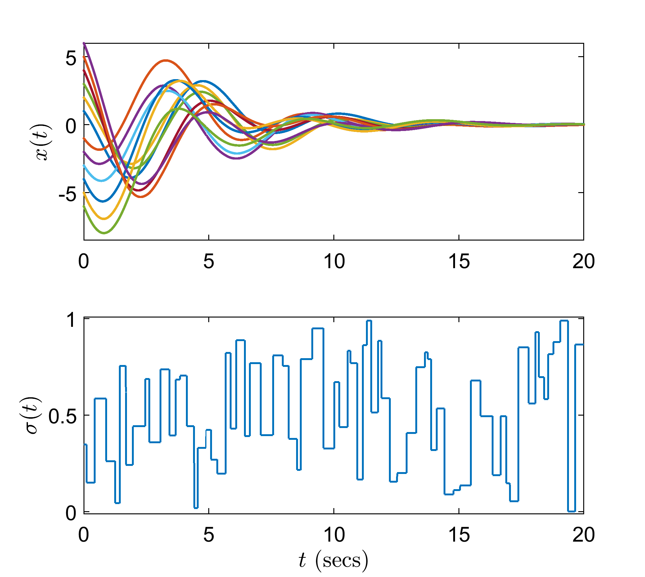
Figure 1: State trajectories (top), switching signal (bottom).

5 Conclusion

It has been shown in this paper that decomposable systems with switching topology can be modeled as LPV systems with a piecewise constant parameter. Then, output feedback stabilizing controllers are designed for these LPV systems in the presence of a time-varying output delay. A trajectory-based approach is used for stability analysis which circumvents the serious obstacle presented by the search for appropriate Lyapunov functionals. No constraint is imposed on the delay derivative. Output feedback control of distributed systems subject to stochastic topology following the idea Zakwan (2020) seems to be one of the promising future extensions of the current work. Moreover, employing different kinds of the controller (e.g., memory or memory resilient) and observer structures (e.g., interval observers) can be quite intriguing. These extensions will be reported elsewhere.

The authors would like to acknowledge useful discussions with Professor Hitay Özbay and Dr. Corentin Briat.

Appendix A Technical Lemmas

In this section, we provide technical lemmas. Lemma 1 highlights an interesting property of decomposable matrices and it is used to prove Theorem 1. Lemma 2 recalls the trajectory based stability analysis approach from Ahmed et al. (2018) and it is used to prove Theorem 3.

Lemma 1

Consider a matrix $M(t)$ with the structure (3) subject to the pattern matrix $\mathcal{P}(t)$ given in (4), then the matrix

$$M^{\dagger}(t)=(U\otimes I_{p})^{-1}M(t)(U\otimes I_{q})$$

is block diagonal and has the following structure

$${M}^{\dagger}(t)=I_{N}\otimes\bar{M}^{a}+\Lambda(t)\otimes\bar{M}^{b}\;,$$ (14)

where each of the block has the form ${M}^{\dagger}_{i}(t)=\bar{M}^{a}+\nu_{i}(t)\bar{M}^{b}$ where $\nu_{i}(t)=\sigma(t)\lambda_{1i}+(1-\sigma(t))\lambda_{2i}$. Moreover, for every matrix $M^{\dagger}(t)$ with the structure (14), we have

$$M(t)=(U\otimes I_{p})M^{\dagger}(t)(U\otimes I_{q})^{-1}=I_{N}\otimes\bar{M}^{a}+\mathcal{P}(t)\otimes\bar{M}^{b}.$$

Proof.

From Definition 1, we can write

$${M}^{\dagger}(t)=(U\otimes I_{p})^{-1}(I_{N}\otimes\bar{M}^{a}+\mathcal{P}(t)\otimes\bar{M}^{b})(U\otimes I_{q})$$

then from the properties of the Kronecker product (Brewer, 1978), we have

$$\begin{array}[]{lll}{M}^{\dagger}(t)=(U^{-1}I_{N}U\otimes I_{p}\bar{M}^{a}I_{q})+(U^{-1}\mathcal{P}(t)U\otimes I_{p}\bar{M}^{b}I_{q})\;.\end{array}$$

As an immediate consequence,

$$\begin{array}[]{lll}{M}^{\dagger}(t)=I_{N}\otimes\bar{M}^{a}+\Lambda(t)\otimes\bar{M}^{b}\;.\end{array}$$

Since $I_{N}$ and $\Lambda(t)$ are diagonal, therefore, ${M}^{\dagger}(t)$ is block diagonal. The converse can be proved analogously. $\hfill\blacksquare$ ∎

Lemma 2 (Ahmed et al., 2018)

Let us consider a constant $T>0$ and $l$ functions $z_{g}:[-T,+\infty)\rightarrow[0,+\infty)$, $g=1,...,l$. Let $Z(t)=(z_{1}(t)\;...\;z_{l}(t))^{\top}$ and, for any $\theta\geq 0$ and $t\geq\theta$, define $\mathfrak{V}_{\theta}(t)=\left(\displaystyle\sup_{s\in[t-\theta,t]}z_{1}(s)\;...\displaystyle\sup_{s\in[t-\theta,t]}z_{l}(s)\right)^{\top}$. Let $\Upsilon\in\mathbb{R}^{l\times l}$ be a nonnegative Schur stable matrix. If for all $t\geq 0$, the inequalities $Z(t)\leq\Upsilon\mathfrak{V}_{T}(t)$ are satisfied, then $\displaystyle\lim_{t\rightarrow+\infty}z_{g}(t)=0~{}~{}~{}\forall~{}g=1,\ldots,l$.

Appendix B Checking Assumption 1

In this section, we illustrate a method to determine the constants $a$, $b$, $c$, and $d$ to satisfy Assumption 1.
Consider an LPV system subject to piecewise parameter trajectory

$$\dot{\xi}(t)=\Omega(\rho)\xi(t)+\vartheta(t)\;,$$ (15)

where $\xi\in\mathbb{R}^{d_{\xi}}$, $\rho\in\mathscr{P}$ and $\vartheta$ is a piecewise continuous function.

Lemma 3

Let the system (15) be such that there are real numbers $d_{1}>0$, $d_{2}>0$, $\mu\geq 1$, $\gamma>0$ and symmetric positive definite matrices $\mathcal{Q}(\rho)$, such that the LMIs

$$d_{1}I\preceq\mathcal{Q}(\rho)\preceq d_{2}I\;,$$ (16)

$$\mathcal{Q}(\rho)\preceq\mu\mathcal{Q}(\theta)\;,$$ (17)

$$\Omega(\rho)^{\top}\mathcal{Q}(\rho)+\mathcal{Q}(\rho)\Omega(\rho)\preceq-\gamma\mathcal{Q}(\rho)$$ (18)

are satisfied for all $\rho,\ \theta\in\mathscr{P}$. Moreover, the constant $\mu_{\triangle}=\mu e^{-\gamma\underline{\delta}}$ is such that

$$\mu_{\triangle}<1\;.$$

Then, along the trajectory of (15), the inequality

$$|\xi(t)|\leq\sqrt{\frac{d_{2}}{d_{1}}\mu\mu_{\triangle}^{\eta}e^{\gamma\overline{\delta}}}|\xi(t-T)|+\sqrt{\mu\frac{d_{2}}{\gamma d_{1}}T}\displaystyle\sup_{\ell\in[t-T,t]}|\vartheta(\ell)|$$

holds for all $t\geq T$ where $T>0$ and $\eta$ is a positive integer depending on the choice of $T$ such that for all $t\in[t_{k},t_{k+1})$, we have $t-T\in[t_{k-\eta-1},t_{k-\eta})$. Moreover, we have $\sqrt{\frac{d_{2}}{d_{1}}\mu\mu_{\triangle}^{\eta}e^{\gamma\overline{\delta}}}<1$ when $\eta>\frac{1}{\ln(\mu_{\Delta})}\left[\ln\left(\frac{d_{1}}{d_{2}\mu}\right)-\gamma\overline{\delta}\right]$.

Appendix C Proofs of the Theorems

In this section, we provide proofs of the theorems appearing in Section 2.

Proof of Threorem 1:.

Using Lemma 1, we can rewrite (1) as

$$\begin{array}[]{lll}(U\otimes I_{n})^{-1}\dot{x}(t)&=&A^{\dagger}(t)(U\otimes I_{n})^{-1}x(t)\\[2.84526pt] &&+B^{\dagger}(t)(U\otimes I_{d_{u}})^{-1}u(t)\\[2.84526pt] (U\otimes I_{d_{y}})^{-1}y(t)&=&C^{\dagger}(t)(U\otimes I_{n})^{-1}x(t)\;.\end{array}$$ (19)

Then, with change of variables $x(t)=(U\otimes I_{n})\hat{x}(t)$, $u(t)=(U\otimes I_{d_{u}})\hat{u}(t)$, and $y(t)=(U\otimes I_{d_{y}})\hat{y}(t)$, it follows from (19) that

$$\begin{array}[]{rcl}\dot{\hat{x}}(t)&=&A^{\dagger}(t)\hat{x}(t)+B^{\dagger}(t)\hat{u}(t)\\[2.84526pt] \hat{y}(t)&=&{C}^{\dagger}(t)\hat{x}(t)\;,\end{array}$$ (20)

where

$$\begin{array}[]{lll}{A}^{\dagger}(t)=I_{N}\otimes\bar{A}^{a}+\Lambda(t)\otimes\bar{A}^{b}\\ {B}^{\dagger}(t)=I_{N}\otimes\bar{B}^{a}+\Lambda(t)\otimes\bar{B}^{b}\\[2.84526pt] C^{\dagger}(t)=I_{N}\otimes\bar{C}^{a}+\Lambda(t)\otimes\bar{C}^{b}\\[2.84526pt] \end{array}$$

are block diagonal matrices. Therefore, the system (20) is equivalent to $N$ independent $nth$ order subsystems given in (6). This concludes the proof. $\hfill\blacksquare$ ∎

Proof of Theorem 2:.

The proof is straightforward and relies on the affine dependence of system matrices on $\nu_{i}$ in (5). Each $\nu_{i}\in[\lambda_{1i},\ \lambda_{2i}]$ can be substituted with a bigger polytope $\rho\in[\min\{\nu_{i}\},\ \max\{\nu_{i}\}]$ for $i=1,2,\ldots,N$. It is obvious that $\min\{\nu_{i}\}=\min\{\underline{\lambda}_{1},\ \underline{\lambda}_{2}\}$. Arguing similarly, we have $\max\{\nu_{i}\}=\max\{\bar{\lambda}_{1},\ \bar{\lambda}_{2}\}$. With these substitutions, the dependence of system matrices on $\nu_{i}$ can be dropped and system of $N$ independent subsystems can be represented by an equivalent LPV system (7). Since the systems (1) and (5) are equivalent according to Theorem 1, the LPV framework (7) captures the dynamics of the system (1). This completes the proof. $\hfill\blacksquare$ ∎

References

• Ahmed et al. (2018) Ahmed, S., Mazenc, F., and Özbay, H. (2018). Dynamic output feedback stabilization of switched linear systems with delay via a trajectory based approach. Automatica, 93, 92–97.
• Atay (2013) Atay, F.M. (2013). The consensus problem in networks with transmission delays. Philosophical Transactions of the Royal Society A, 371(1999), 1–13.
• Betser et al. (2005) Betser, A., Vela, P.A., Pryor, G., and Tannenbaum, A. (2005). Flying in formation using a pursuit guidance algorithm. In Proceedings of the American Control Conference, 5085 – 5090.
• Borrelli and Keviczky (2008) Borrelli, F. and Keviczky, T. (2008). Distributed LQR design for identical dynamically decoupled systems. IEEE Transactions on Automatic Control, 53(8), 1901 – 1912.
• Brewer (1978) Brewer, J. (1978). Kronecker products and matrix calculus in system theory. IEEE Transactions on circuits and systems, 25(9), 772–781.
• Briat (2015a) Briat, C. (2015a). Linear Parameter-Varying and Time-Delay Systems – Analysis, Observation, Filtering & Control. Springer-Verlag, Berlin-Heidelberg.
• Briat (2015b) Briat, C. (2015b). Stability analysis and control of a class of LPV systems with piecewise constant parameters. Systems & Control Letters, 82, 10–17.
• Carpenter (2000) Carpenter, J.R. (2000). A preliminary invetigation of decentralized control for satellite formations. In Proceedings of the IEEE Aerospace Conference, 63 – 74.
• Eichler et al. (2014) Eichler, A., Hoffmann, C., and Werner, H. (2014). Robust control of decomposable LPV systems. Automatica, 50(12), 3239–3245.
• Ghadami and Shafai (2013) Ghadami, R. and Shafai, B. (2013). Decomposition-based distributed control for continuous-time multi-agent systems. IEEE Transactions on Automatic Control, 58(1), 258–264.
• Ghaedsharaf et al. (2016) Ghaedsharaf, Y., Siami, M., Somarakis, C., and Motee, N. (2016). Interplay between performance and communication delay in noisy linear consensus networks. In Proceedings of the European Control Conference, 1703 – 1708.
• Gonzalez and Werner (2014) Gonzalez, A.M. and Werner, H. (2014). LPV formation control of non-holonomic multi-agent systems. IFAC Proceedings Volumes, 47(3), 1997–2002.
• Horn and Johnson (2012) Horn, R.A. and Johnson, C.R. (2012). Matrix Analysis. Cambridge University Press, NY, USA.
• Jiang et al. (2006) Jiang, S., Voulgaris, P.G., Holloway, L.E., and Thompson, L.A. (2006). Distributed control of large segmented telescopes. In Proceedings of the American Control Conference, 1942 – 1947.
• Jovanovic and Bamieh (2005) Jovanovic, M.R. and Bamieh, B. (2005). On the ill-posedness of certain vehicular platoon control problems. IEEE Transactions on Automatic Control, 50(9), 1307 – 1321.
• Li and Duan (2014) Li, Z. and Duan, Z. (2014). Cooperative Control of Multi-agent Systems: A Consensus Region Approach. Taylor & Francis Group, Boca Raton, FL, USA.
• Löfberg (2004) Löfberg, J. (2004). YALMIP: A toolbox for modeling and optimization in MATLAB. In Proceedings of the IEEE International Symposium on Computer Aided Control Systems Design, 284–289.
• Massioni and Verhaegen (2009) Massioni, P. and Verhaegen, M. (2009). Distributed control for identical dynamically coupled systems: A decomposition approach. IEEE Transactions on Automatic Control, 54(1), 124–135.
• Mesbahi and Hadaegh (2001) Mesbahi, M. and Hadaegh, F.Y. (2001). Formation flying control of multiple spacecraft via graphs, matrix inequalities, and switching. Journal of Guidance, Control, and Dynamics, 24(2), 369 – 377.
• Olfati-Saber and Murray (2004) Olfati-Saber, R. and Murray, R.M. (2004). Consensus problems in networks of agents with switching topology and time-delays. IEEE Transactions on Automatic Control, 49(9), 1520 – 1533.
• Papachristodoulou et al. (2010) Papachristodoulou, A., Jadbabaie, A., and Munz, U. (2010). Effects of delay in multi-agent consensus and oscillator synchronization. IEEE Transactions on Automatic control, 55(6), 1471 – 1477.
• Qiao and Sipahi (2016) Qiao, W. and Sipahi, R. (2016). Consensus control under communication delay in a three-robot system: Design and experiments. IEEE Transactions on Control Systems Technology, 24(2), 687 – 694.
• Seuret et al. (2008) Seuret, A., Dimarogonas, D.V., and Johansson, K.H. (2008). Consensus under communication delays. In Proceedings of the 47th IEEE Conference on Decision and Control, 4922 – 4927.
• Stewart et al. (2003) Stewart, G.E., Gorinevsky, D.M., and Dumont, G.A. (2003). Feedback controller design for a spatially distributed system: The paper machine problem. IEEE Transactions on Control Systems Technology, 11(5), 612 – 628.
• Sturm (1999) Sturm, J.F. (1999). Using sedumi 1.02, a MATLAB toolbox for optimization over symmetric cones. Optimization Methods and Software, 11(1-4), 625–653.
• Sun and Wang (2009) Sun, Y.G. and Wang, L. (2009). Consensus of multi-agent systems in directed networks with nonuniform time-varying delays. IEEE Transactions on Automatic Control, 54(7), 1607 – 1613.
• Zakwan (2020) Zakwan, M. (2020). Dynamic $L_{\text{2}}$ output feedback stabilization of LPV systems with piecewise constant parameters subject to spontaneous poissonian jumps. IEEE Control Systems Letters, 4(2), 408–413.
• Zakwan and Ahmed (2020) Zakwan, M. and Ahmed, S. (2020). Distributed output feedback control of decomposable LPV systems with delay and switching topology: Application to consensus problem in multi-agent systems. International Journal of Control, DOI:10.1080/00207179.2019.1710257.
• Zhou and Lin (2014) Zhou, B. and Lin, Z. (2014). Consensus of high-order multi-agent systems with large input and communication delays. Automatica, 50(2), 452–464.