Instability and phase transitions of a rotating black hole
in the presence of perfect fluid dark matter

Abstract

In this paper, we study the thermodynamic features of a rotating black hole surrounded by perfect fluid dark matter. We analyze the critical behavior of the black hole by considering the known relationship between pressure and cosmological constant. We show that the black hole admits a first order phase transition and, both rotation and perfect fluid dark matter parameters have a significant impact on the critical quantities. We also introduce a new ad hoc pressure related to the perfect fluid dark matter and find a first order van der Waals like phase transition. In addition, using the sixth order WKB method, we investigate the massless scalar quasinormal modes (QNMs) for the static spherically symmetric black hole surrounded by dark matter. Using the finite difference scheme, the dynamical evolution of the QNMs is also discussed for different values of angular momentum and overtone parameters.

I Introduction

Black hole thermodynamics continues to be a promising topic of gravitational physics as it is one of the possible routes towards quantum gravity. The idea of relating black holes and ordinary thermodynamics was notably founded by Bekenstein and Hawking and subsequently carried on by other researchers. More recently the idea of thermodynamics of anti-de Sitter (AdS) black holes has got unusual attention by the discovery of gauge-gravity (AdS/CFT) correspondence mal . Hawking and Page found the existence of a phase transition between the stable Schwarzschild black hole and the pure radiation or gas page . Later it was found that there exists a small-large black hole phase transition for charged or rotating AdS black holes cha1 ; cha2 . This phase transition is also identified with the liquid-gas phase transition of the van der Waals fluid mann . We can work in the extended phase space thermodynamics and use the key identification between the cosmological constant and the pressure by $P\sim\Lambda$, and its conjugate variable as the thermodynamic volume PV1 ; PV2 .

In literature, the critical phenomenon and the phase transition of several AdS black holes in various gravitational setups have already been explored. The first order phase transition for five dimensional charged AdS black holes was investigated in wei . Similar critical behavior was also observed for the AdS black hole in massive gravity sf . A more general treatment of phase transitions for extremal black holes was proposed in p without considering any specific black hole. Wei and Liu proposed an interesting connection between the impact parameter of the photon orbits and the thermodynamic phase transitions of charged AdS black holes wei2 . They suggested that the changes of the photon sphere radius and the minimum impact parameter can serve as order parameters for a small-large black hole phase transition.

Thermodynamics of Kerr-AdS black hole in four and higher dimensions is discussed in Ref. Altamirano:2014tva . It is shown that in the canonical ensemble (fixed angular momentum), four dimensional rotating AdS black hole behaves qualitatively similar to the charged AdS case with fixed angular momentum replacing fixed charge. The critical point for every fixed angular momentum can be determined numerically. They demonstrated that in the regime of slow rotation, a van der Waals type phase transition takes place. In Czinner:2017tjq , the Rényi approach is used to study thermodynamics of Kerr black hole. In this approach, all the thermodynamic quantities are obtained using R$\acute{e}$nyi entropy rather than Bekenstein-Hawking entropy. It is shown that the characteristic swallow-tail behavior is observed for the definite Rényi entropy parameter, which is corresponding to a small/large black hole phase transition analogous to the picture of rotating black holes in AdS space.

It is worth mentioning the possibility of studying the extended phase space from the viewpoint of AdS/CFT correspondence. In this mechanism, the AdS radius relates to the number of colors in the dual gauge theory. So, variable cosmological constant is equivalent to variable number of colors Kubiznak:2016qmn . Moreover, the thermodynamic volume may be interpreted as associated chemical potential for the color. It is known that changing the sign of chemical potential is an indication of quantum effects. This subject has been studied in Maity:2015ida for Kerr-AdS black holes in four and five dimensions. It is shown that the sign of chemical potential is changed above the Hawking-Page transition temperature which is physically dual to a confinement-deconfinement transition of the boundary gauge theory.

On the other hand, it is interesting to study the effect of surroundings on the thermodynamics of rotating black hole. The Kerr black hole in the presence of electromagnetic field is considered in Ref. Liao:2016mum . The authors explored the parameter condition for superconducting phase transition and obtained an appropriate value for the ratio of mass squared over angular momentum so that Meissner effect occurs. In other words, conditions for existence/non-existence of Meissner effect phase transition is discussed. Phase transition for the Kerr-Newman-AdS black hole in quintessence matter as a model of dark energy is discussed in Jafarzade:2017wtc . Extension of the model including nonlinear magnetic charge is given in Ndongmo:2019ywh . In this paper, we are interested to explore the effect of dark matter on the rotating black holes.

It is suggested that about $27$ % of our universe is made from the invisible dark matter. One of the main evidence for this idea is the galaxy’s flat rotation curve Rubin . The dependence of rotation velocity on the distance from the center of spiral galaxies has an asymptotically flat character in contrast to the expectations from Newton’s law, while the strong dominated gravitational field due to the presence of dark matter in far distances can explain this observation. For an explanation of this dark halo contribution, Kiselev presented a new class of solutions of the Einstein equation, by applying the perfect fluid relations, and introduced a new logarithmic term which explains the observed asymptotic behavior at large distances kiselev . Li & Yang proposed a model of black hole immersed in dark matter halo in the presence of dark energy modeled as inhomogeneous phantom field yang . They extended the Kiselev solution to the exact static spherically solution consistent with the Schwarzschild-AdS and Reissner-Nordström metrics. Later Xu et al generalized these solutions to the Kerr dS/AdS black holes surrounded by the perfect fluid dark matter using the Janis-Newman algorithm xu1 . In literature, astrophysical aspects of this black hole have already been studied such as shadow images and the geodetic precession frequency sum ; r .

In this paper, we are interested to investigate how the presence of perfect fluid dark matter affect the thermodynamical/dynamical aspects of black holes. We examine dynamical stability with quasi-normal modes (QNMs) along with thermal stability and possible phase transition.

Regarding different black hole solutions of gravitating systems, the examination of instability conditions is a strong tool to veto some models. In order to obtain the stability criteria and investigate the stability of a black hole, one should examine its response to dynamic and thermodynamic perturbations. On the one hand, the behavior of the heat capacity is one of the powerful tools to analyze thermal stability. It is shown that in the canonical ensemble (fixed charged) the positivity of heat capacity can guarantee (local) thermal stability. On the other hand, the QNMs RW can reflect the behavior of black holes under dynamic perturbations QNM1 ; QNM2 ; QNM3 ; QNM4 . After the detection of the gravitational radiation of compact binary mergers by LIGO and VIRGO observatories GW1 ; GW2 ; GW3 , investigation of QNMs attracted much attention. This is due to the fact that the spectrum of gravitational QNMs perturbations can be traced by gravitational wave detectors PRL . In this paper, we restrict ourselves to the case of scalar perturbation.

The plan of the paper is as follows: In section II, we discuss the thermodynamical properties of the black hole under consideration. The phase transitions analysis is performed in section III. We then investigate QNMs for the static black hole in section IV, and finally, conclude in section V.

II Rotating perfect fluid dark matter black hole and its thermodynamics

We consider a black hole with rotation immersed in a perfect fluid background sum

$$ds^{2}=-\frac{\Delta_{r}}{\rho^{2}\Sigma}(dt-a\sin^{2}\theta d\phi)^{2}+\frac{\Delta_{\theta}\sin^{2}\theta}{\rho^{2}\Sigma}(adt-(r^{2}+a^{2})d\phi)^{2}+\frac{\Sigma}{\Delta_{r}}dr^{2}+\frac{\Sigma}{\Delta_{\theta}}d\theta^{2},$$

where

$$\Delta_{r} = r^{2}-2Mr+a^{2}-\frac{\Lambda}{3}r^{2}(r^{2}+a^{2})+\alpha r\ln(r/|\alpha|),$$

$$\Delta_{\theta} = 1+\frac{\Lambda}{3}a^{2}\cos^{2}\theta,$$

$$\rho = 1+\frac{\Lambda}{3}a^{2},$$

$$\Sigma = r^{2}+a^{2}\cos^{2}\theta.$$ (1)

The logarithmic term in the metric is responsible for presence of dark matter and the intensity of the PFDM is presented by the parameter $\alpha$. We see that this solution reduces to the Kerr-AdS metric as we set $\alpha=0$.

The mass of the black hole is determined by the condition $\Delta_{r}(r_{+})=0$, so

$$M=\frac{1}{2}\Big{[}r_{+}+\frac{a^{2}}{r_{+}}-\frac{\Lambda}{3}r_{+}(r_{+}^{2}+a^{2})+\alpha\log\Big{(}\frac{r_{+}}{|\alpha|}\Big{)}\Big{]}.$$ (2)

Regarding asymptotically dS solutions (left panel of Fig. 1), the event horizon $r_{+}$, inner horizon $r_{-}$ and cosmological horizon $r_{c}$ of black hole satisfy $\Delta_{r}(r_{+})=\Delta_{r}(r_{-})=\Delta_{r}(r_{c})=0$, so we can use the position of horizons to replace the parameters $M$, $a$ and $\Lambda$. In addition, the behavior of asymptotically AdS solutions is shown in the right panel of Fig. 1. Briefly, the relation between $\Delta_{r}$ and $r$ with different $\alpha$ is shown in Fig. 1.

$\begin{array}[]{cc}\includegraphics[width=227.62204pt]{dShorizon.eps}&\includegraphics[width=227.62204pt]{AdShorizon.eps}\end{array}$

Figure 1: $\Delta_{r}$ versus $r$ with different $\alpha$, where $r_{+}=1$, $r_{-}=1/2$: (left panel: dS solutions with $r_{c}=5$ and right panel: AdS solutions with $\Lambda=-1$).

The area of event horizon of the black hole is given by

$$A=4\pi\frac{(r_{+}^{2}+a^{2})}{\rho}.$$ (3)

Therefore the Bekenstein-Hawking entropy relation becomes

$$S=\frac{A}{4}=\pi\frac{(r_{+}^{2}+a^{2})}{\rho},$$ (4)

and Hawking temperature associated with the surface gravity of the event horizon $r_{+}$ is determined as:

$$T_{h}=\frac{r_{+}}{4\pi\rho(r_{+}^{2}+a^{2})}\Big{[}1-\frac{a^{2}}{r_{+}^{2}}-\frac{\Lambda}{3}(3r_{+}^{2}+a^{2})+\frac{\alpha}{r_{+}}\Big{]}.$$ (5)

III Phase transitions

In this section, we are going to examine possible phase transition. Following the traditional $PV$ criticality in the extended phase space, we can regard the cosmological constant as a dynamical pressure, $\Lambda=-8\pi P$. Considering Eq. (5), it is straightforward to obtain the following equation of state

$$P=\frac{3}{8\pi a^{2}}\left[\frac{4\pi T(r_{+}^{2}+a^{2})-(r_{+}+\alpha)+\frac{a^{2}}{r_{+}}}{4\pi T(r_{+}^{2}+a^{2})+r_{+}+\frac{3r_{+}^{3}}{a^{2}}}\right].$$ (6)

Here, we can identify the specific volume $v$ as $v=2r_{+}$ in the geometric units. Therefore, as it is usual, we use the event horizon radius instead of the specific volume in order to analyze the criticality. Due to the fact that the critical point in the isothermal $P-r_{+}$ is an inflection point, we can find the critical quantities with the following equations

$$\left(\frac{\partial P}{\partial r_{+}}\right)_{T}=0,\text{ \ \ \ \ \ \ }\left(\frac{\partial^{2}P}{\partial r_{+}^{2}}\right)_{T}=0.$$ (7)

Since the analytical calculation of the critical quantities is not a trivial task, we use the numerical analysis. Using Eq. (7), the critical point can be found numerically. Regarding the functional form of the pressure, one finds that its denominator can be vanished for some values of the event horizon radius (we called largest ones as $r_{+d}$). Investigating such divergencies with more details, we find that the pressure is negative for $r_{+}<r_{+d}$, and therefore, we study the positive pressure region, $r_{+}>r_{+d}$. Looking at Fig. 2, we find the van der Waals like behavior for the solution, and therefore, a first order phase transition has been occurred for $T<T_{c}$. The critical values for the mentioned black hole solutions are addressed in table I. In this table, we focus on the effects of $a$ and $\alpha$. It is observed that increasing the rotation parameter (decreasing $\alpha$) leads to increasing the critical horizon radius and decreasing the critical temperature and pressure. In other words, the effect of $a$ and $\alpha$ on the critical quantities is opposed to each other. It means that the criticality is easier to see for highly rotating black holes with vanishing $\alpha$. In Ref. Altamirano:2014tva , by approximating the equation of state in the regime of slow rotation, one can find that decreasing the rotation parameter leads to increasing the critical pressure and temperature (decreasing the critical radius) which is consistent with our results in the table I. Influence of perfect fluid dark matter on the thermodynamic behavior of Reissner-Nordström-AdS black hole is investigated in Ref. Xu:2016ylr . In the mentioned paper, phase transition is discussed in charge squared-electric potential plane and a resemblance to the van der Waals system is found.

$\begin{array}[]{cc}\includegraphics[width=227.62204pt]{PVaa01alpha001.eps}&\includegraphics[width=227.62204pt]{PVaa01alpha005.eps}\end{array}$

Figure 2: Pressure versus $r_{+}$ for $a=0.01$ and $\alpha=0.001$ (left panel), and $\alpha=0.005$ (right panel).

$a$     $r_{c}$      $T_{c}$      $P_{c}$ $0.01$ $0.0295$ $3.423$ $20.75$ $0.05$ $0.1529$ $0.6501$ $0.7578$ $0.10$ $0.3073$ $0.3229$ $0.1873$ $0.20$ $0.6160$ $0.1610$ $0.0465$

$\alpha$     $r_{c}$      $T_{c}$      $P_{c}$ $0.005$ $0.02482$ $4.455$ $32.58$ $0.010$ $0.02052$ $6.186$ $55.38$ $0.030$ $0.01268$ $19.56$ $253.6$ $0.050$ $0.01000$ $55.70$ $596.8$

Table I: Left table: critical values for $\alpha=0.001$ with different rotation parameter.

Right table: critical values for $a=0.01$ with different $\alpha$.

To get more information about the phase transition, we study thermodynamic quantities such as heat capacity and Gibbs free energy. Using the standard definition, they are as follows

$$C_{P}=T\frac{\partial S}{\partial T}\bigg{|}_{\Lambda,a,\alpha}=\frac{6\pi(a^{2}+r_{+}^{2})\left(8\pi P(r_{+}^{2}+\frac{a^{2}}{3})+1+\frac{\alpha}{r_{+}}-\frac{a^{2}}{r_{+}^{2}}\right)}{(8\pi Pa^{2}-3)\left(-8\pi P(r_{+}^{2}+\frac{8a^{2}}{3}+\frac{a^{4}}{3r_{+}^{2}})+1+\frac{2\alpha}{r_{+}}-\frac{a^{2}}{r_{+}^{2}}(4+\frac{a^{2}}{r_{+}^{2}})\right)},$$ (8)

$$G=M-TS=-\frac{r_{+}\left(1-\frac{a^{2}}{r_{+}^{2}}+\frac{8}{3}\pi P(a^{2}+3r_{+}^{2})+\frac{\alpha}{r_{+}}\right)}{4\left(1+\frac{\Lambda a^{2}}{3}\right)\left(1-\frac{8}{3}\pi Pa^{2}\right)}+\frac{1}{2}\left(r_{+}+\frac{a^{2}}{r_{+}}+\frac{8}{3}\pi Pr_{+}(a^{2}+r_{+}^{2})+\alpha\ln(\frac{r_{+}}{|\alpha|})\right).$$ (9)

$\begin{array}[]{cc}\includegraphics[width=227.62204pt]{c-r-a01alpha001.eps}&\includegraphics[width=227.62204pt]{c-r-a01alpha005.eps}\end{array}$

Figure 3: Heat capacity versus $r_{+}$ for $a=0.01$ and $\alpha=0.001$ (left panel), and $\alpha=0.005$ (right panel).

$\begin{array}[]{cc}\includegraphics[width=227.62204pt]{G-T-a01alpha001.eps}&\includegraphics[width=227.62204pt]{G-T-a01alpha005.eps}\end{array}$

Figure 4: Gibbs free energy versus $T$ for $a=0.01$ and $\alpha=0.001$ (left panel), and $\alpha=0.005$ (right panel).

In Fig. 3, we can find heat capacity behavior versus critical radius $r_{+}$ for definite parameters. As we expect from the first order phase transition, there are two divergencies for pressures less than the critical pressure, which are seen by red and blue colors. Negative heat capacity in this region indicates unstable black hole, which is equivalent to the oscillations of the isotherms under critical temperature in the $P-r_{+}$ diagram (Fig. 2). These divergencies are characteristics of the first order phase transition between small and large black holes which are stable with positive heat capacity. By changing the parameter $\alpha$, a shift in the horizontal axis occurs, which as mentioned before, increasing this parameter results to decreasing of critical radius.

Gibbs free energy versus temperature is plotted in Fig. 4. The swallow-tail behavior for pressures less than critical pressure, indicates a first order transition. Besides, we see by increasing parameter $\alpha$, critical temperature increases and phase transition occurs as before.

Here, we are looking for the possible phase transition with vanishing or constant $\Lambda$. To do so, we can define the following ad hoc relation for the pressure

$$P=\frac{|\alpha|}{r_{+}^{3}}.$$ (10)

As one confirms, this pressure is related to the event horizon radius which is the same as the pressure of black holes in dilaton gravity. Inserting Eq. (10) into the relation of temperature, one finds

$$P=\frac{4\pi T}{r_{+}}\left(1+\frac{a^{2}}{r_{+}^{2}}\right)\left(1+\frac{\Lambda a^{2}}{3}\right)+\frac{1}{r_{+}^{2}}\left(-1+\frac{\Lambda a^{2}}{3}\right)+\Lambda+\frac{a^{2}}{r_{+}^{4}}.$$ (11)

Having the equation of state at hand, we are in a position to obtain the critical quantities via Eq. (7), as

$$r_{c} = \frac{-a\sqrt{6\Gamma(\Gamma-\Theta-6)}}{2\Gamma},$$ (12)

$$T_{c} = \frac{\sqrt{6}\Gamma^{2}(\Gamma-\Theta-2)}{6\pi a(\Gamma+6)(3\Gamma-\Theta-6)\sqrt{\Gamma\left(\Gamma-\Theta-6\right)}},$$ (13)

$$P_{c} = \frac{2}{9}\frac{\Gamma^{2}}{a^{2}(\Gamma-\Theta-6)}\left[1+\frac{2}{(\Gamma-\Theta-6)}\left(1-\frac{(\Gamma-\Theta-2)(5\Gamma-3\Theta-18)}{3(3\Gamma-\Theta-6)}\right)\right]+\Lambda,$$ (14)

where $\Gamma=\Lambda a^{2}-3$ and $\Theta=\sqrt{\Lambda^{2}a^{4}-26\Lambda a^{2}+105}$.

Now, we are going to investigate the possible phase transition based on $P-r_{+}$ diagrams (see Fig. 5). According to this figure, we observe a van der Waals like behavior which hints us for a first order phase transition. According to table II, one can find the effects of rotation parameter and cosmological constant. It is seen that unlike the rotation parameter, the cosmological constant does not have a considerable effect on the critical quantities. However, as we mentioned before, increasing the rotation parameter leads to obtaining the criticality easier.

$a$     $r_{c}$      $T_{c}$      $P_{c}$ $0.01$ $0.03102$ $3.098$ $454.2$ $0.05$ $0.1551$ $0.6198$ $18.08$ $0.10$ $0.3102$ $0.3101$ $4.446$ $0.20$ $0.6202$ $0.1554$ $1.038$ $0.30$ $0.9297$ $0.1040$ $0.4072$

$\Lambda$     $r_{c}$      $T_{c}$      $P_{c}$ $-0.4$ $0.31008$ $0.31077$ $4.1530$ $-0.3$ $0.31012$ $0.31053$ $4.2506$ $-0.2$ $0.31015$ $0.31030$ $4.3483$ $-0.1$ $0.31018$ $0.31007$ $4.4459$ $0$ $0.31022$ $0.30983$ $4.5435$

Table II: Left table: critical values for $\Lambda=-0.1$ with different rotation parameter.

Right table: critical values for $a=0.1$ with different $\Lambda$.

$\begin{array}[]{cc}\includegraphics[width=227.62204pt]{Lminus01a01.eps}&\includegraphics[width=227.62204pt]{Lminus01a02.eps}\end{array}$

Figure 5: Pressure versus $r_{+}$ for $\Lambda=-0.1$ and $a=0.1$ (left panel), and $a=0.2$ (right panel).

$\begin{array}[]{cc}\includegraphics[width=170.71652pt]{c-r-a01landaminus01P001pc10T.eps}&\includegraphics[width=170.71652pt]{c-r-a01landaminus01P001pc10p5T.eps}\end{array}$

Figure 6: Heat capacity versus $r_{+}$ for $\Lambda=-0.1$, $a=0.1$ and $P=0.01P_{c}$, which shows divergencies in two different regions. The dashed line corresponds to $10T$ (right panel) and $10^{5}T$(left panel).

$\begin{array}[]{cc}\includegraphics[width=170.71652pt]{c-r-a02landaminus01P004pc10T.eps}&\includegraphics[width=170.71652pt]{c-r-a02landaminus01P004pc10p5T.eps}\end{array}$

Figure 7: Heat capacity versus $r_{+}$ for $\Lambda=-0.1$, $a=0.2$ and $P=0.04P_{c}$, which shows divergencies in two different regions. The dashed line corresponds to $10T$ (right panel) and $10^{5}T$(left panel).

$\begin{array}[]{cc}\includegraphics[width=227.62204pt]{G-T-a01landaminus01.eps}&\includegraphics[width=227.62204pt]{G-T-a02landaminus01.eps}\end{array}$

Figure 8: Gibbs free energy versus $T$ for $\Lambda=-0.1$ and $a=0.1$ (left panel), and $\Lambda=-0.1$ and $a=0.2$ (right panel).

Heat capacity and Gibbs free energy are given, respectively, as

$$C_{P}=\frac{6\pi r_{+}^{2}(a^{2}+r_{+}^{2})\left((\Lambda-P)r_{+}^{2}+\frac{1}{3}\Lambda a^{2}-1+\frac{a^{2}}{r_{+}^{2}}\right)}{(3+\Lambda a^{2})\left((\Lambda+2P)r_{+}^{4}+(\frac{8}{3}\Lambda a^{2}+1)r_{+}^{2}+(\frac{\Lambda a^{2}}{3}-4)a^{2}-\frac{a^{4}}{r_{+}^{2}}\right)},$$ (15)

$$G=\frac{(\Lambda-P)r_{+}^{3}+\left(\frac{\Lambda a^{2}}{3}-1\right)+\frac{a^{2}}{r_{+}}}{4\left(\frac{\Lambda a^{2}}{3}+1\right)^{2}}+\frac{r_{+}}{2}\left(1+\frac{a^{2}}{r_{+}^{2}}-\frac{1}{3}\Lambda(a^{2}+r_{+}^{2})-Pr_{+}^{2}\ln(|P|r_{+}^{2})\right).$$ (16)

It is interesting to see the characteristic behaviors of the first order phase transition by the ad hoc definition for pressure (Eq. (10)). Two divergencies for the heat capacity are shown for different regions and parameters in Figs. 6 and 7. The physical black holes with positive heat capacity and temperature are seen just before the first divergency and after the second one.

The swallow-tail like form of the Gibbs free energy for these two figures is shown in Fig. 8, which assures existence of the first order phase transition by defining pressure as Eq. (10).

IV Quasi-normal modes of a static PFDM black hole

Let us consider the perturbation around the black hole background. The black hole perturbations or quasinormal modes are a vital source of gravitational waves generated as a result of a supernova collapse. Numerous simulations of gravitational collapse of a rotating massive star and merger of binary compact star system result in the emission of gravitational waves which are directly linked with quasinormal mode oscillations QNM2 . The process of field oscillations in the curved background includes three phases: initial perturbation, quasinormal mode oscillations and the ensuing tails. The properties of oscillations just depend on the second and third phases, so the study of QNM oscillations and tails can help to understand the nature of black holes PRL . In the QNM oscillation phase, the function of field equation could be written as $\Psi\sim e^{-i\omega t}R(r)Y(\theta,\varphi)$ where $\omega$ is the eigenvalue whose real and imaginary parts represent frequency and decay rate of QNM perturbations respectively, so that the imaginary part should be negative for stable black hole spacetime. The real part of the QNM frequency denoted by $\omega_{R}$ determines the oscillation frequency while the imaginary part $\omega_{I}$ determines the rate at which each mode is damped as a result of emission of radiation. With the help of spherical harmonics, one can write $\Delta Y(\theta,\varphi)=-L(L+1)Y(\theta,\varphi)$, where $L$ denotes multipole quantum number. Since different black hole spacetimes in different gravitational theories produce different QNMs frequency, so investigating the details of QNMs is important and helpful to discriminate different modified gravities or test the instability of black hole solution. In the ensuing computations, we shall ignore cosmological constant and the rotation for simplicity reasons.

To study quasinormal modes, we focus on the following static metric yang

$$ds^{2}=-f(r)dt^{2}+\frac{dr^{2}}{f(r)}+r^{2}(d\theta^{2}+\sin^{2}\theta d\phi^{2}),$$ (17)

where

$$f(r)=1-\frac{2m}{r}+\frac{\alpha}{r}\ln\Big{(}\frac{r}{|\alpha|}\Big{)}.$$ (18)

For computational and analytical simplicity, we employ the following relation for the mass of black hole using Eq. (18) : $2m=r_{h}+\alpha\ln\Big{(}\frac{r_{h}}{|\alpha|}\Big{)}$, which allows rewriting the above equation as

$$f(r)=1-\frac{r_{h}}{r}+\frac{\alpha}{r}\ln\Big{(}\frac{r}{|\alpha|}\Big{)}-\frac{\alpha}{r}\ln\Big{(}\frac{r_{h}}{|\alpha|}\Big{)}=1-\frac{1}{x}-\frac{b}{x}\ln(x),$$ (19)

and entails $f(r_{h})=0$, where $r_{h}=r_{+}$ denotes the size of horizon radius, and $x=r/r_{h}$, $\alpha=-b\;r_{h}$. Interestingly, $r_{h}$ is event horizon as $b<1$, while it becomes inner horizon as $b>1$, see left panel of Fig. 9. As $b=0$, the black hole becomes the Schwarzschild black hole, and the temperature of black hole vanishes as $b=1$. As $b>0$, the position $x_{b}=e^{1-1/b}$ which satisfies $f^{\prime}(x_{b})=0$ is less than the event horizon, but as $b<0$, $x_{b}$ is larger than the event horizon so that a maximum value exists outside the event horizon, see right panel of Fig. 9. We find the form of $f(r)$ with a maximum point which is similar to non-Schwarzschild solution in quadratic and higher derivative gravity k1a ; k1b ; k1c .

$\begin{array}[]{ccc}\includegraphics[width=227.62204pt]{fx.eps}&&\includegraphics[width=227.62204pt]{Relation.eps}\end{array}$

Figure 9: The relation between $b$ and $f(x)$ (left) and the relation between $b$ and $x_{b}$ (right).

We consider a massless scalar perturbation in the background of the black hole spacetime. The equation of motion of a minimally coupled scalar field is given by:

$$\nabla^{\mu}\nabla_{\mu}\Phi=0.$$ (20)

We express the scalar field in the form of separation of variables i.e. $\Phi(x^{\mu})=\sum\frac{\Psi_{L}(r)}{r}Y_{Lm}(\theta,\phi)e^{-i\omega t}$. Since we are dealing with spherically symmetric spacetimes the solution will be independent of m, thus this subscript can be omitted. Introducing the tortoise coordinate $r_{*}=\int\frac{dr}{f(r)},$ having range between $(-\infty,+\infty)$, it is possible to write the radial part of the wave equation (also known as Regge-Wheeler form) as follows

$$\frac{d^{2}\Psi}{dr_{*}^{2}}+[\omega^{2}-V(r)]\Psi(r_{*})=0,$$ (21)

where the effective potential is given as

$$V(r)=f(r)\Big{(}\frac{f^{\prime}(r)}{r}+\frac{L(L+1)}{r^{2}}\Big{)}.$$ (22)

$\begin{array}[]{cc}\includegraphics[width=170.71652pt]{Vforb1.eps}&\includegraphics[width=170.71652pt]{VforbNeg1.eps}\\ \includegraphics[width=170.71652pt]{Vforb05.eps}&\includegraphics[width=170.71652pt]{VforbNeg05.eps}\end{array}$

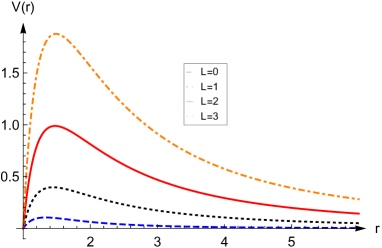
Figure 10: $V(r)$ versus $r$ for $b=1$ (up-left panel), $b=-1$ (up-right panel), $b=0.5$ (middle-left panel), $b=-0.5$ (middle-right panel) and $b=0$ (down panel).

$\begin{array}[]{cc}\includegraphics[width=170.71652pt]{VforL0.eps}&\includegraphics[width=170.71652pt]{VforL1.eps}\\ \includegraphics[width=170.71652pt]{VforL2.eps}&\includegraphics[width=170.71652pt]{VforL3.eps}\end{array}$

Figure 11: $V(r)$ versus $r$ for $L=0$ (up-left panel), $L=1$ (up-right panel), $L=2$ (down-left panel) and $L=3$ (down-right panel).

There are numerous numerical approaches for determining the solution, known as quasinormal modes with complex frequencies, of the above wave equation (see QNM4 ). However, we shall use the sixth order Wentzel-Kramers-Brillouin (WKB) approximation method to calculate the quasinormal modes. The WKB method was originally proposed by Schutz, and Iyer and Will at third order, independently will1 ; will2 while later was extended to sixth order in kono . This approach is useful to obtain the QNMs for a full range of parameters and has the best accuracy for $L\geq n$. In general, for a given effective potential $V(r)$, the sixth order WKB formula has the form

$$\frac{i(\omega^{2}-V_{0})}{\sqrt{-2V_{0}^{\prime\prime}}}-\sum_{i=2}^{6}\Lambda_{i}=n+\frac{1}{2},$$

where $V_{0}$ denotes the numerical value of the effective potential evaluated at the peak (or the maximum) while similarly $V_{0}^{\prime\prime}$ denotes the corresponding second derivative evaluated at the maximum. Also, the correction terms $\Lambda_{i}$’s are corresponding to the the i-th order of WKB method depending on the value of the effective potential, $V(r)$ and its derivatives at the local maximum will2 ; kono , and $n$ is the overtone number.

Considering the functional form of $V(r)$ and Figs. 10 and 11, we find that the effective potential is constant at the boundaries (the event horizon and the infinity), and it rises to a maximum at an intermediate point $r=r_{0}$. Acceptable accuracy of the (sixth order) WKB method is guaranteed since such a method is based on the matching of WKB expansion of the wave function at the boundaries with the Taylor expansion near the local maximum of the potential barrier through the two turning points. In other words, WKB method can be used for an effective potential that forms a potential barrier and takes constant values at the boundaries (See Figs. 10 and 11 for more details regarding the effect of different parameters on the peak of the potential).

From the Figs. 12, we have plotted the real and imaginary components of oscillation frequency against parameter $b$ and shown that QNMs perturbation will increase but the damping of QNMs is faster as $b$ reduces. Further, $\omega_{I}<0$ depicting that black hole configuration is stable after perturbation.

$\begin{array}[]{cc}\includegraphics[width=227.62204pt]{wR.eps}&\includegraphics[width=227.62204pt]{wI.eps}\end{array}$

Figure 12: Scalar quasinormal modes of the black hole for different values of angular (or multipole) quantum number $L$ and overtone $n$.

$\begin{array}[]{cc}\includegraphics[width=227.62204pt]{QNMsL0.eps}\includegraphics[width=227.62204pt]{QNMsL1.eps}\\ \includegraphics[width=227.62204pt]{QNMsL2.eps}\includegraphics[width=227.62204pt]{QNMsL3.eps}\end{array}$

Figure 13: Dynamical evolution of a scalar field perturbation to the black hole.

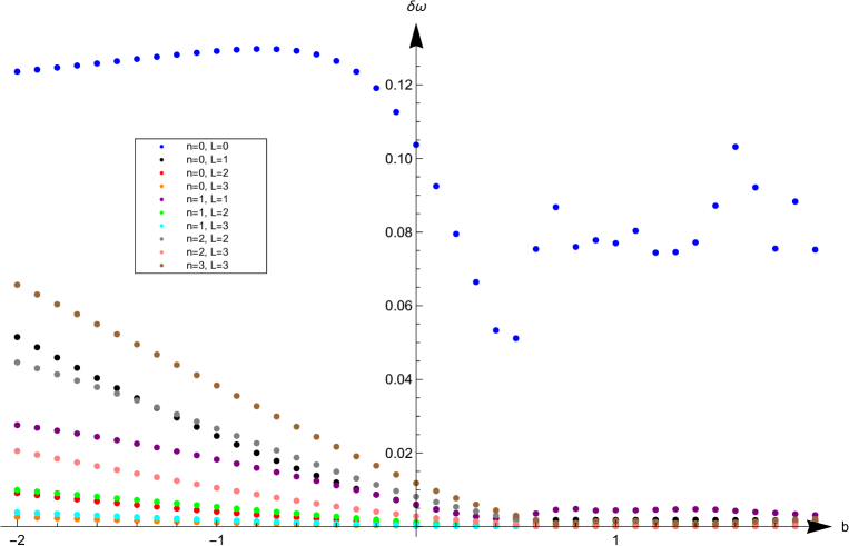
Figure 14: A plot showing relative errors between WKB methods of order 6 and 3.

In order to study the dynamical properties of QNMs perturbation, we show the details of black hole oscillations by using finite difference method following jin . Firstly, we rewrite Eq.(21) as

$$\frac{\partial^{2}\Phi}{\partial r_{*}^{2}}-\frac{\partial^{2}\Phi}{\partial t^{2}}=V(r)\Phi.$$ (23)

After the transformation $u=t-r_{*}$ and $v=t+r_{*}$, above equation becomes

$$\frac{\partial^{2}\Phi}{\partial u\partial v}+\frac{1}{4}V(r)\Phi=0.$$ (24)

Therefore, we can use finite difference method to solve above equation and show the process of black hole oscillations in Fig. 13. The oscillations are damped for fixed $L$ and three values of $b$. In each figure, it is observed that $b=-1$ case has the fastest damping ending up in a tail, followed by $b=0$ which has a rather slow damping speed with an observed tail while $b=1$ has the slowed decaying rate. In Fig. 14, we have plotted relative errors between the WKB methods of order $3$ and $6$, by defining a parameter

$$\delta\omega\equiv|\frac{\omega_{6}-\omega_{3}}{\omega_{6}}|,$$

where $\omega_{3}$ and $\omega_{6}$ are the values of QNM frequencies obtained by the WKB method of orders $3$ and $6$, respectively. For different values of parameters $n$ and $L$, the relative error in absolute form $\delta\omega$ increases along negative $b-$axis, while along positive $b-$axis the relative error $\delta\omega$ decreases and both orders of WKB method give same kind of approximation to QNM frequencies. In summary, the errors are very small with order less than $0.1$, hence the numerical analysis is considered to be credible.

V Conclusion

In this paper, we considered the Kerr-AdS black hole surrounded by the perfect fluid dark matter (PFDM). We have done a detailed analysis of the effect of PFDM on the thermodynamical behavior of this kind of black holes. By giving dynamics to the cosmological constant and it’s association with pressure i.e. $P=\frac{-\Lambda}{8\pi}$, we worked in the extended phase space to study the phase behavior. We found the van der Waals like behavior for the solution and by a numerical method, we observed that increasing the rotation parameter (decreasing $\alpha$) leads to increasing the critical horizon radius and decreasing the critical temperature and pressure. Two divergencies in the $C_{P}-r_{+}$ plots and the swallow-tail shape in the $G-T$ plots for pressures less than the critical pressure indicate that these black holes enjoy the first order phase transition.

On the other hand, by dimensional analysis, we proposed another relation for the pressure $P=\frac{|\alpha|}{r_{+}^{3}}$. In this case, pressure is related to the PFDM parameter and the horizon radius. Analytic relations for the critical quantities are found and the results show that unlike the rotation parameter, the cosmological constant does not have a considerable effect on the critical quantities. However, as before, increasing the rotation parameter leads to obtaining the criticality easier. Interestingly, we observe that this ad hoc definition for the pressure also results in the first order phase transition for the introduced black hole solutions.

In the last part, we studied the QNMs for the static metric in the presence of the PFDM. Using the sixth order WKB method, we investigated the massless scalar quasinormal modes (QNMs) for the static spherically symmetric black hole surrounded by dark matter. Using the finite difference scheme, the dynamical evolution of the QNMs are also discussed for different values of angular momentum and overtone parameters. The QNM oscillations are damped in all cases of considered $L$ and $b$, however for $b=-1,0$, the damping is faster as compared to $b=1$. Here we ignored the effects of cosmological constant and spin while studying the QNMs, however one may employ the method of Horowitz-Hubeny hh to analyze QNM frequencies for static black holes with AdS boundary. This is left as future work.

Since the spectrum of gravitational QNMs perturbations can be traced by gravitational wave detectors, it will be interesting to study the response of the solutions under tensor perturbation. This work may be addressed in independent work.

References

- (1) J.M. Maldacena, Adv. Theor. Math. Phys. 2, 231 (1998).
- (2) S.W. Hawking and D.N. Page, Comm. Math. Phys. 87, 577 (1983).
- (3) A. Chamblin, R. Emparan, C.V. Johnson and R.C. Myers, Phys. Rev. D 60, 064018 (1999).
- (4) A. Chamblin, R. Emparan, C.V. Johnson and R.C. Myers, Phys. Rev. D 60, 104026 (1999).
- (5) D. Kubiznak and R.B. Mann, JHEP 1207, 033 (2012).
- (6) D. Kastor, S. Ray and J. Traschen, Class. Quantum Gravit. 26, 195011 (2009).
- (7) B.P. Dolan, Class. Quantum Gravit. 28, 125020 (2011).
- (8) S.W. Wei, B. Liang and Y.X. Liu, Phys. Rev. D 96, 124018 (2017).
- (9) S. Fernando, Phys. Rev. D 94, 124049 (2016).
- (10) K. Bhattacharya, S. Dey, B. Majhi and S. Samanta, Phys. Rev. D 99, 124047 (2019).
- (11) S.W. Wei and Y.X. Liu, Phys. Rev. D 97, 104027 (2018).
- (12) N. Altamirano, D. Kubiznak, R. B. Mann and Z. Sherkatghanad, Galaxies 2, 89 (2014).
- (13) V. G. Czinner and H. Iguchi, Eur. Phys. J. C 77, 892 (2017).
- (14) D. Kubiznak, R. B. Mann and M. Teo, Class. Quant. Grav. 34, 063001 (2017).
- (15) R. Maity, P. Roy and T. Sarkar, Phys. Lett. B 765, 386 (2017).
- (16) Y. Liao, X. B. Gong and J. S. Wu, Astrophys. J. 835, 247 (2017).
- (17) K. Jafarzade and J. Sadeghi, arXiv:1710.08642 [hep-th].
- (18) R. T. Ndongmo, S. Mahamat, T. B. Bouetou and T. C. Kofane, arXiv:1911.12521 [gr-qc].
- (19) V.C. Rubin, Jr.W.K. Ford and N. Thonnard, Astrophys. J. 238, 471 (1980).
- (20) V.V. Kiselev, [arXiv:gr-qc/0303031].
- (21) M.H. Li and K.C. Yang, Phys. Rev. D 86, 123015 (2012).
- (22) Z. Xu, X. Hou and J. Wang, Class. Quantum Gravit. 35, 115003 (2018).
- (23) S. Haroon, M. Jamil, K. Jusufi, K. Lin, R.B. Mann, Phys. Rev. D 99, 044015 (2019).
- (24) M. Rizwan, M. Jamil, K. Jusufi, Phys. Rev. D 99, 024050 (2019).
- (25) T. Regge and J.A. Wheeler, Phys. Rev. 108, 1063 (1957).
- (26) S. Chandrasekhar, The Mathematical Theory of Black Holes, Cambridge University Press (1983).
- (27) K.D. Kokkotas and B.G. Schmidt, Living Rev. Rel. 2, 2 (1999).
- (28) E. Berti, V. Cardoso and A.O. Starinets, Class. Quantum Gravit. 26, 163001 (2009).
- (29) R.A. Konoplya and A. Zhidenko, Rev. Mod. Phys. 83, 793 (2011).
- (30) B.P. Abbott et al. [LIGO Scientific and Virgo Collaborations], Phys. Rev. Lett. 116, 061102 (2016).
- (31) B.P. Abbott et al. [LIGO Scientific and Virgo Collaborations], Phys. Rev. Lett. 116, 221101 (2016).
- (32) B.P. Abbott et al. [LIGO Scientific and Virgo Collaborations], Phys. Rev. Lett. 116, 241103 (2016).
- (33) M. Isi, M. Giesler, W.M. Farr, M.A. Scheel and S.A. Teukolsky, Phys. Rev. Lett. 123, 111102 (2019).
- (34) Z. Xu, X. Hou, J. Wang and Y. Liao, Adv. High Energy Phys. 2019, 2434390 (2019) (2009).
- (35) K. Lin, A.B. Pavan, G. Flores-Hidalgo and E. Abdalla, Braz. J. Phys. 47, 419 (2017).
- (36) H. Lu, A. Perkins, C.N. Pope and K.S. Stelle, Phys. Rev. Lett. 114, 171601 (2015).
- (37) K. Lin, W.L. Qian, A. B. Pavan and E. Abdalla, Europhys. Lett. 114, 60006 (2016).
- (38) B.F. Schutz and C.M. Will, Astrophys. J. 291, L33 (1985).
- (39) S. Iyer and C.M. Will, Phys. Rev. D 35, 3621 (1987).
- (40) R.A. Konoplya, Phys. Rev. D 68, 024018 (2003).
- (41) J. Li, H. Ma and K. Lin, Phys. Rev. D 88, 064001 (2013).
- (42) G.T. Horowitz and V.E. Hubeny, Phys. Rev. D 62, 024027 (2000).