Leslie’s prey-predator model in discrete time
Abstract.
We consider the Leslie’s prey-predator model with discrete-time. This model is given by a non-linear evolution operator depending on five parameters. We show that this operator has two fixed points and define type of each fixed point depending on the parameters. Finding two invariant sets of the evolution operator we study the dynamical systems generated by the operator on each invariant set. Depending on the parameters we classify the dynamics between a predator and a prey of the Leslie’s model.
Key words and phrases:
population, Leslie model, prey-predator, discrete-time.2010 Mathematics Subject Classification:
34D20 (92D25)1. Introduction
First predator-prey models were introduced by Lotka and Volterra. These models have been extensively studied by mathematical and biological researchers. The investigations are important in understanding the dynamics between a predator and a prey (population with two species), which live together in the same environment (see [4], [5], [6], [13], [18], [19] and references therein). One interests for a suitable conditions that allow the both species survive in equilibria [15]. But in many papers (see for example [9]-[12]) have shown that considering a harvesting term in the model can lead to the extinction of any species.
Following [5] consider the Leslie’s prey-predator model in continuous time. At time moment consider the following model:
| (1.1) |
where and are positive parameters. The predator equation is logistic, with carrying capacity proportional to the prey population. This two species food chain model describes a prey population which serves as food for a predator . This model usually studied for continuous time.
In this paper (as in [14] and [16]) we study a model of discrete time process of Leslie’s prey-predator model (1.1), which has the following form
| (1.2) |
where and
We are interested to the behavior of the sequence , for any initial point .
The paper is organized as follows. In Section 2 we construct two invariant sets with respect to operator . Section 3 devoted to fixed points of the operator, moreover the type of each fixed point is defined depending on the parameters of the model. In Section 4 under some conditions on parameters we give limit points of trajectories. In the last section we give numerical analysis of trajectories corresponding to the remaining cases of parameters.
2. Invariant sets
The set is called an invariant with respect to operator if We formulate the following:
Proposition 1.
The set
is an invariant with respect to .
The proof of this Proposition is straightforward.
Definition 1.
(see. [7], page 47) Let and be two maps. and are said to be topologically conjugate if there exists a homeomorphism such that, . The homeomorphism is called a topological conjugacy.
Under a condition on parameters the restriction of the operator on is topologically conjugate to the well-known quadratic family (discussed in [7]). Let us do this point clear: in the system (1.2), if then from the first equation we get
Proposition 2.
Two maps and are topologically conjugate for .
Proof.
We take the linear map and by Definition 1 we should have i.e.,
from this identity we get
Thus, the homeomorphism is Moreover, since we have ∎
The importance of this proposition is that if two maps are topologically conjugate then they have essentially the same dynamics (see. [7], page 53).
Proposition 3.
Let Then the set
is an invariants with respect to operator if
(1) or
(2) and .
Proof.
If then by we have
and by the form of we have
Similarly,
Next we show that
Case-1. If then . Hence, in this case and is an invariant.
Case-2. Let we consider the inequality Instead of we put their expressions and we have
Last inequality is always true with respect to if a discriminant is nonpositive, i.e.,
By solving this inequality we obtain the (2) condition of the Proposition.Thus the proposition is proved. ∎
Remark 1.
The conditions (to the parameters ) in Proposition 3 are sufficient for the set to be an invariant.
3. Fixed points
A fixed point ([14]) for a mapping is a solution to the equation . We will study fixed points of the operator (1.2). Let be an initial point. By the continuity of the operator , (1.2), the limit points of each trajectory are fixed points for the operator .
Proposition 4.
For the operator (1.2) fixed points are
and
where (if then from second inequality we get that and .)
Proof.
i) If then the equation , (where ) has the solution .
ii) If then the system of equations has unique solution and here for
existence of fixed point we have conditions and . If then
| (3.1) |
from this we get , but all parameters are positive, so and there is no solution of the system (3.1). ∎
Proposition 5.
The following relations hold
-
(1)
-
(2)
where
Proof.
(1) First we find the Jacobian for the system (1.2):
| (3.2) |
Then the Jacobian at the fixed point has the form
and the eigenvalues of this matrix are . By solving inequalities , we get , thus, is an attracting fixed point. The proof of all other cases are similar.
(2) The Jacobian at the second fixed point has the following form
.
Then the eigenvalues of this matrix are the roots of the following quadratical equation:
∎
We note that there exist coefficients satisfying the condition For example, if then
4. Limit points
4.1. Definitions
The set of limit points of trajectory is very important in the theory of dynamical systems, so we will study the set of limit points of trajectories of the operator (1.2).
Definition 2.
(see. [7], page 49) is said to be topologically transitive if for any pair of open sets there exists such that
Definition 3.
(see. [7], page 49) has sensitive dependence on initial conditions if there exists such that, for any and any neighborhood of , there exists and such that
Definition 4.
(see. [7], page 50) is said to be chaotic on if
1. has sensitive dependence on initial conditions;
2. is topologically transitive;
3. periodic points are dense in
4.2. On the invariant set
Consider trajectories on the invariant set first.
Proposition 6.
If and initial point then
Proof.
If then , from this we get Thus,
since In addition, by conjugacy of the operators , and by Proposition 5.3. (in [7], page 32) from we have In Proposition 1, since , so and going to the limit from two sides we have , where If then for any (where is the set of all positive integers), i.e., the sequence monotonically decreasing. Since the sequence is bounded from below, it has a limit. The limit should be a fixed point for the function , i.e. the unique fixed point . Hence, as
We note that, by the domain of the operator (1.2), ∎
Proposition 7.
Let .
(i) has an attracting fixed point and repelling fixed point 0.
(ii) If then
Proof.
(i). Let with . Then it has two fixed points: and We have and . Hence 0 is a repelling for and is an attracting with .
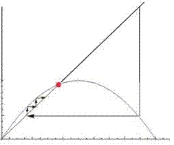
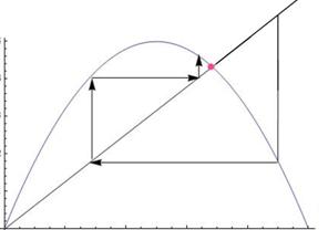
(ii) Case: Suppose Then graphical analysis (which is called Kyonigsa-Lamereya diagram, see [17], page 7) shows that If lies in the interval then lies in , so that the previous argument implies (see Fig.2)
Case: Graphical analysis shows what is different in this case (see Fig.2). Note that Let denote the unique point in the interval that is mapped onto by Then we can easily check that maps the interval inside It follows that as for all Now suppose Again graphical analysis shows that there exists integer such that Thus as Similarly, maps the interval onto Since , we have finished the proof. ∎
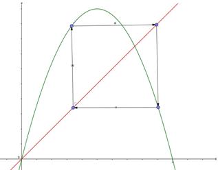
If then the fixed point becomes repelling. Let us consider 2-periodical points of the function (see Fig.4) as roots of the equation:
Then we have the following solutions: , We know that if then the cycle is an attracting (see [17], page 9). Hence,
then , if
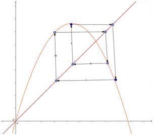
If then the cycle becomes repelling. Numerical analysis shows that if then there exists four periodical attracting cycle (see Fig.4).
Proposition 8.
Let Then
(i) If then the operator has a cycle of period two;
(ii) If then the operator has a cycle of period four;
(iii) If then the operator has a cycle of period eight;
(iv) If then has chaotic dynamics for any initial point
Proof.
The proof of (i), (ii) and (iii) follows from above mentioned discussion. Proof of the (iv) follows by the arguments of [7], pages 50-51. ∎
4.3. On the invariant set
Theorem 1.
Let be an initial point and
(i) If then
(ii) If then there exists a neighborhood such that
Proof.
For we get and from this
If then . Thus, is decreasing and it has a limit. We assume that
From second equation of the operator we have:
From this we obtain This is a contradiction to the boundedness of the sequence in the invariant set Hence,
Case-(i). If we get and
If then It means than the sequence monotone decreasing and it has limit If we assume that then it must be a fixed point. But in this case there is no fixed point of the operator Thus,
Case-(ii). Above we have shown that independently on the sequence has zero limit and if
Let now First equation of the operator is:
| (4.1) |
For by Proposition 7 we get that the limit of the sequence is .
Theorem 2.
Let be an initial point which is not fixed points and let . Then
(i) If then the operator converges to a cycle of period two;
(ii) If then the operator converges to a cycle of period four;
(iii) If then the operator converges to a cycle of period eight;
(iv) If then has chaotic dynamics.
Proof.
By the condition we have that It means that for any initial point there exists such that the operators and have the same limit behavior. Hence, proof of this theorem follows from Proposition 8.∎
Let us give some figures related to this Theorem: If then by two periodical points , which are mentioned in above, we have two attracting fixed points of period 2. For example, if then and (Fig. 7). Similarly, for the , for example, , we can see the behavior of the trajectory with respect to the attracting cycle of period four (Fig.7). In addition, represented 8, 16 and greater periodical fixed points. (Fig. 9, Fig. 9, Fig. 11, Fig. 11).
5. Case
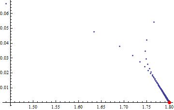
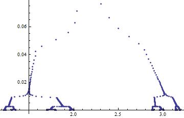
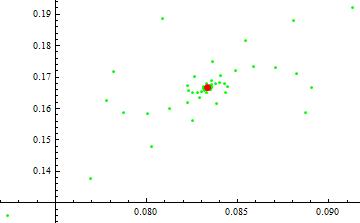
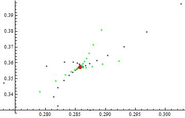
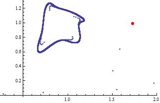
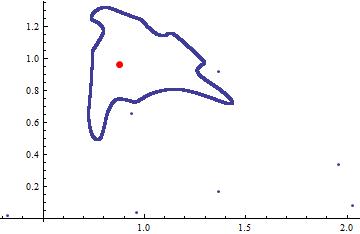
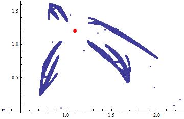
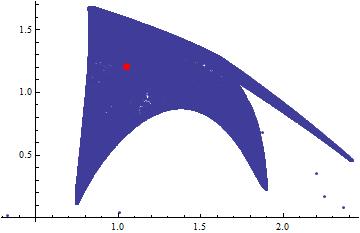
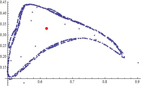
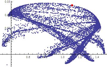
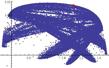
In this case we have several interesting cases, in particular chaos. Numerical analysis shows that the coordinates of the vector are not monotone, so it is not easy to see the limit properties of the trajectory. Therefore, we study these limits numerically for concrete values of parameters: (In all Figures the red point is the fixed point )
5.1. Numerical analysis.
1) Then by the system (1.2) we get
| (5.1) |
For this system Here we choose the initial point with condition . By using Wolfram Mathematica 7.0 we find limit points of initial point (Fig.13).
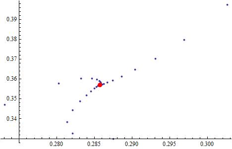
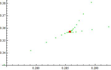
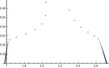
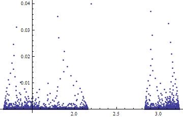
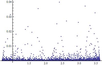
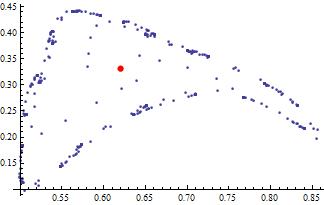
2) Then after iteration we have with . (Fig.15) We see that in some subcases of the system (1.2) limit is:
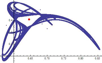
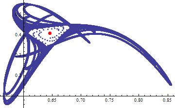
But for some cases the behavior of the trajectory is various (Fig.19- Fig.22).
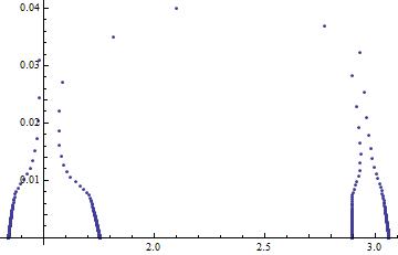
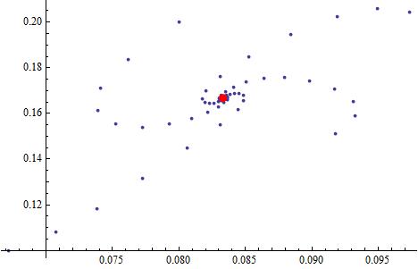
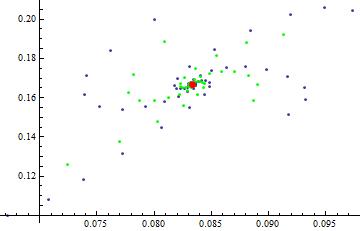
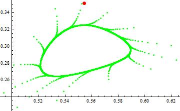
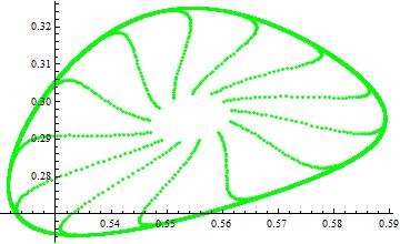
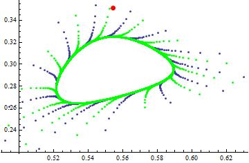
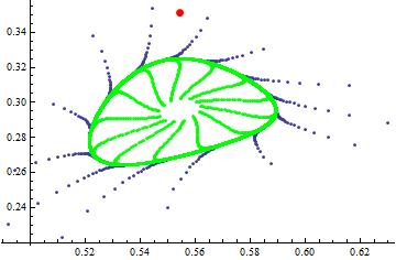
4) For the trajectory is given in Fig.21 and Fig.22 From the Fig.21 and Fig.22 we can say that in this case there is an invariant domain which is bounded by closed and attracting invariant curve.
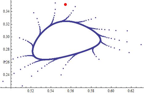
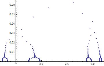
5) For the trajectory is given in Fig.26
6) For the trajectory is given in Fig.26
7) For the trajectory is given in Fig.28
8) For the trajectory is given in Fig.28
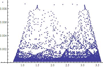
5.2. Lyapunov exponents
It is known that the Lyapunov exponents describe the behavior of vectors in the tangent space of the phase space and are defined from the Jacobian matrix, ([2], [3], [8], [20]).
Lyapunov exponent is calculated by eigen values of the limit of the following expression:
where tends to infinity, and is the Jacobian of the function at the iterated point . For the evaluation of Lyapunov exponent, we have taken an initial point and iterated it say for 106 time so that we are closer to the fixed point. We find where say and calculate the Eigenvalues of that resultant matrix. Then is the Lyapunov exponent.
For the system (1.2) we consider the case and we calculate the Lyapunov exponent. The Jacobian is:
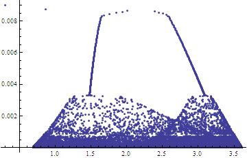
Then
Acknowledgements
Shoyimardonov thanks the "El-Yurt Umidi" Foundation under the Cabinet of Ministers of the Republic of Uzbekistan for financial support during his visit to the University of Montpellier (France) and prof. R.Varro for the invitation.
References
- [1] K. Alligood, T. Sauer, and J. Yorke. An Introduction to Dynamical Systems. In New York: Spinger-Verlag, 1997.
- [2] H.D.I Arardonel, R. Brown and M.B. Kennel. Local Lyapunov Exponents Computed from Observed Data. In J. Nonlinear Science, pages 175–199. 1991.
- [3] D.K. Arrowsmith and C.M. Place. An Introduction to Dynamical Systems. In Cambridge Unversity Press, 1994.
- [4] M.A. Aziz-Alaoui. Study of a Leslie-Gower-type tritrophic population model. In Chaos, Solitons and Fractals, pages 1275–1293. 2002.
- [5] N. Britton. Essential Mathematical Biology. In Springer, London, 2003.
- [6] Y. Chow, S.R.-J. Jang. Asymptotic dynamics of a modified discrete Leslie-Gower competition system. In Int. J. Biomath, 23 pp. 2017.
- [7] R.L. Devaney. An Introduction to Chaotic Dynamical System. In Westview Press, 2003.
- [8] L. Diect, R. D. Russell, E. S. Van Vleck. On the Computation of Lyapunov Exponents for Continuous Dynamical Systems. In SIAM Journal, Numer. Anal, pages 402–423, 34(1) (1997).
- [9] R.N. Ganikhodzhaev. Quadratic stochastic operators, Lyapunov functions and tournaments. In Russian Acad. Sci.Sb. Math, pages 489–506. 76 (1993).
- [10] R.N. Ganikhodzhaev, F.M. Mukhamedov, U.A. Rozikov. Quadratic stochastic operators and processes: results and open problems. In Inf. Dim. Anal. Quant. Prob. Rel. Fields, pages 279–335, 14(2) (2011).
- [11] R.P. Gupta, P. Chandra, M. Banerjee. Dynamical complexity of a preypredator model with nonlinear predator harvesting. In Discr. Cont. Dyn. Sys., Series B,pages 423–443, 20(2) (2015).
- [12] R. C. Hilborn. Chaos and Nonlinear Dynamics, An Introduction For Scientists and Engineers. In Oxford University Press, 1994.
- [13] J. Müller, C. Kuttler. Methods and models in mathematical biology. In Deterministic and stochastic approaches. Lecture Notes on Mathematical Modelling in the Life Sciences. Springer, Heidelberg, 2015.
- [14] U.A. Rozikov, S.K. Shoyimardonov. Ocean ecosystem discrete time dynamics generated by Volterra operators. In Inter. Jour. Biomath. 12(2) (2019) 24 pages.
- [15] U.A. Rozikov, J.B. Usmonov. Dynamics of a population with two equal dominated species. In arXiv:1909.07106 [math.DS], 2019.
- [16] U.A. Rozikov, M.V. Velasco. A discrete-time dynamical system and an evolution algebra of mosquito population. In J. Math. Biol. pages 1225–1244, 78(4) (2019).
- [17] A.N. Sharkovskii, S.F. Kolyada, A.G. Sivak, V.V. Fedorenko. Dynamics of one-dimentional maps. In Kiev, Naukova Dumka, 1989.
- [18] R. Sivasamy, K. Sathiyanathan, K. Balachandran. Dynamics of a modified Leslie-Gower model with gestation effect and nonlinear harvesting. In J. Appl. Anal. Comput, pages 747–764, 9(2) (2019).
- [19] S. Slimani, P.F. Raynaud, I. Boussaada. Dynamics of a prey-predator system with modified Leslie-Gower and Holling type II schemes incorporating a prey refuge. In Discrete Contin. Dyn. Syst. Ser. B, pages 5003–5039, 24(9) (2019).
- [20] H.M. Wu. The Hausdroff dimension of chaotic sets generated by a continuous map from into itself. In J. South China Univ. Natur. Sci. Ed., pages 45–51, 2002.