Universal survival probability for a $d$-dimensional run-and-tumble particle

Abstract

We consider an active run-and-tumble particle (RTP) in $d$ dimensions and compute exactly the probability $S(t)$ that the $x$-component of the position of the RTP does not change sign up to time $t$. When the tumblings occur at a constant rate, we show that $S(t)$ is independent of $d$ for any finite time $t$ (and not just for large $t$), as a consequence of the celebrated Sparre Andersen theorem for discrete-time random walks in one dimension. Moreover, we show that this universal result holds for a much wider class of RTP models in which the speed $v$ of the particle after each tumbling is random, drawn from an arbitrary probability distribution. We further demonstrate, as a consequence, the universality of the record statistics in the RTP problem.

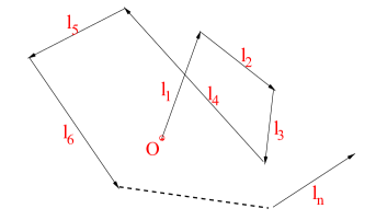
Figure 1: Typical trajectory of a RTP in two dimensions. The particle starts at the origin $O$, chooses a random direction and moves ballistically in that direction for a distance $l_{1}=v_{0}\,\tau_{1}\,,$ where $v_{0}$ is constant and $\tau_{1}$ is a random time drawn from the exponential distribution $p(\tau)=\gamma\,e^{-\gamma\tau}$. At the end of this first flight, the particle tumbles instantaneously and chooses a new random direction and again moves ballistically a distance $l_{2}=v_{0}\tau_{2}$ with $\tau_{2}$ drawn independently from the same $p(\tau)$. Then the particle tumbles again and so on.

The first time $t_{\rm f}$ at which a stochastic process reaches a fixed target level is a fundamental observable with many applications. Statistics of $t_{\rm f}$ plays a crucial role in various situations, including e.g., the encounter of two molecules in a chemical reaction HTB90 , the capture of a prey in a hunting scenario BLMV11 , or the escape of a comet from the solar system Ham61 ; BF_2005 . In the context of finance, agents often use limit orders to buy/sell a stock only when its price is below/above a target value. Thus, it is important to estimate if and when that target value will be reached and this question has been intensively studied during decades (for recent reviews see BLMV11 ; Redner_book ; SM_review ; Persistence_review ; fp_book_2014 ; Masoliver_book ). Due to the ubiquity of these problems, novel applications are constantly being identified, raising in turn new challenging questions.

In recent years, tremendous efforts have been devoted to the study of statistical fluctuations in active matter systems Marchetti13 ; Bechinger16 ; Ram17 ; Sch03 . In contrast to a passive matter such as a Brownian motion (BM), whose dynamics is driven by thermal fluctuations of the environment, this class of active non-equilibrium systems is characterized by self-propelled motility based on continuous consumption of energy from the environment. For example, models of active matter have been used to describe vibrating granular matter WW_2017 , active gels R_2010 ; NVG2019 , bacteria Berg_book ; Cates_bacteria or collective motion of “animals” R_2010 ; V_1995 ; HB_2004 ; VZ12 . In this context, one of the most studied model is the run-and-tumble particle (RTP) TC_2008 ; CT_2015 , also known as “persistent random walk” Weiss_2002 ; ML_2017 . In the simplest version of the model, an RTP performs a ballistic motion along a certain direction at a constant speed $v_{0}\geq 0$ (“run”) during a certain “time of flight” $\tau$. Following this run, it “tumbles”, i.e., chooses a new direction uniformly at random and then performs a new run along this direction again with speed $v_{0}$ during a random time $\tau$ and so on (see Fig. 1). Typically these tumblings occur with constant rate $\gamma$, i.e. the $\tau$’s of different runs are independently distributed via exponential distribution $p(\tau)=\gamma e^{-\gamma\tau}$, though other distributions will also be considered later. Despite its simplicity, this RTP model exhibits complex interesting features such as clustering at boundaries Bechinger16 , non-Boltzmann distribution in the steady state in the presence of a confining potential TC_2008 ; Dhar_18 ; Sevilla_19 ; MBE2019 ; 3states_19 , motility-induced phase separation CT_2015 , jamming SEB2016 etc. Variants of the RTP model where the speed $v\geq 0$ of the particle is renewed after each tumbling by drawing it from a probability density function (PDF) $W(v)$ GM_2019 ; footnote_andrea or where the RTP undergoes random resetting to its initial position at a constant rate EM_2018 ; M2019 have also been studied.

In the $d=1$ case, the first-passage properties of the RTP model and of its variants have been widely studied Weiss_2002 ; artuso14 ; Malakar_2018 ; DM_2018 ; LDM_2019 . Several recent studies investigated the survival probability of an RTP in $d=1$, both in the absence and in the presence of a confining potential/wall Malakar_2018 ; DM_2018 ; LDM_2019 ; ADP_2014 ; Dhar_18 . The $d=1$ case is analytically tractable because the velocity has only two possible directions $\pm v_{0}$, which simplifies the problem in $d=1$. However, in $d>1$, the first-passage problems become much more difficult because the orientation of the velocity is a continuous variable. Consequently, exact results are difficult to obtain in $d\geq 2$, though approximation schemes have been developed recently for the mean first-passage time in a confined geometry RBV16 .

In this Letter we consider an RTP in $d$-dimensions, starting from the origin with a random velocity, and compute exactly the probability $S(t)$ that the $x$-component of the RTP does not change sign up to time $t$. It is useful to view $S(t)$ as the “survival probability” of the RTP in the presence of an absorbing hyperplane passing through the origin and perpendicular to the $x$-axis. For a passive particle executing Brownian motion (BM), it is clear that $S(t)$ is independent of $d$, since each component of the displacement performs an independent one-dimensional BM footnote_BM . In contrast, for an RTP in $d$ dimensions, the different spatial components are coupled (see Fig. 1) and, consequently one may expect that $S(t)$ would depend on the dimension $d$ and the speed $v_{0}$. Performing first simulations in $d=1,2,3$ (see Fig. 2) we found, rather amazingly, that $S(t)$ is completely independent of both $d$ and $v_{0}$, at any finite time $t$ (and not just at large times only) !

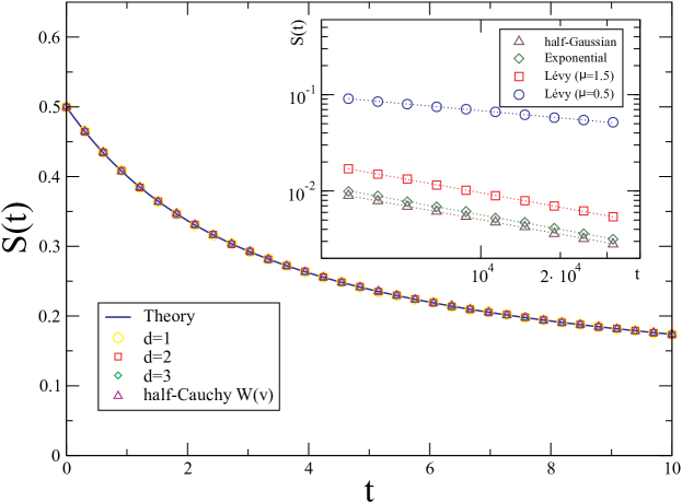
Figure 2: Survival probability $S(t)$ as a function of time $t$, for $\gamma=1$. The continuous blue line corresponds to the exact result in Eq. (1). The symbols correspond to simulations with the choices $d=1,2,3$, $W(v)=\delta(v-1)$ and $p(\tau)=e^{-\tau}$ and one case where $d=2$, $W(v)=2/(\pi(1+v^{2}))$ with $v>0$ (half-Cauchy) and $p(\tau)=e^{-\tau}$. They all fall on the analytical blue line for all $t$. Inset: Numerical computation of $S(t)$ in $d=2$ for different distributions $p(\tau)$: (i) half-Gaussian, (ii) exponential, (iii) asymmetric Lévy distribution with Lévy index $\mu=3/2$ and (iv) asymmetric Lévy with $\mu=1/2$. In all these cases, $S(t)\sim t^{-\theta}$ for large $t$ with $\theta=\frac{1}{2}$ in cases (i)-(iii) and $\theta=\mu/2=1/4$ for case (iv) corresponding to $\mu=1/2$.

The principal goal of this Letter is to understand and prove this remarkably universal result valid even at finite $t$. We compute $S(t)$ exactly for all $t$ in arbitrary dimension $d$, and demonstrate that it is indeed independent of the dimension $d$ and speed $v_{0}$ for any time $t$ and is given by a simple formula

$$S(t)=\frac{1}{2}e^{-\gamma t/2}\left(I_{0}\left(\gamma t/2\right)+I_{1}\left(\gamma t/2\right)\right)\;,$$ (1)

where $I_{0}(z)$ and $I_{1}(z)$ are modified Bessel functions. When $t\rightarrow 0$, $S(t)$ goes to the limiting value $1/2$, which is just the probability that the $x$-component of the initial direction is positive. On the other hand, at late times it decays as $S(t)\sim 1/\sqrt{\pi\gamma t}$. By mapping our $d$-dimensional process to an effective $1d$-process we show below that the universality of this result (1) is inherited from the universality of the Sparre Andersen (SA) theorem SA_54 for the survival probability of a one-dimensional discrete-time random walk. In the special case $d=1$, as a bonus, we recover here using a completely different method, the result in Eq. (1) obtained in previous works Weiss_2002 ; Malakar_2018 ; LDM_2019 via Fokker-Planck approaches. In Fig. 2, we compare our formula for $S(t)$ in (1) with numerical simulations for $d=1,2$ and $3$, finding an excellent agreement at all $t$. Furthermore, this universal result (1) also holds for a broader class of RTP models where the speed $v$, and not just the direction, is also renewed afresh after each tumbling, chosen each time independently from the PDF $W(v)$, with $v\in[0,\infty)$. The standard RTP model corresponds to the choice $W(v)=\delta(v-v_{0})$ but this also includes fat tailed PDF $W(v)$ such as the half-Cauchy distribution: $W(v)=2/[\pi\,(1+v^{2})]$ ($v\geq 0$), as shown in Fig. 2 . Our main result thus states that for the most common RTP model with exponentially distributed time of flights $p(\tau)=\gamma e^{-\gamma\tau}$, the survival probability $S(t)$ at all $t$ is not only independent of the dimension $d$, but also on the velocity distribution $W(v)$ and is given by Eq. (1). We further show that this universal behavior ceases to hold if the distribution of the $\tau$’s is not an exponential. In fact, if $p(\tau)$ has a well defined first moment then one still has $S(t)\propto t^{-1/2}$ at large times but $S(t)$ is not universal for finite time $t$. Finally, for very fat tailed distribution such that the first moment is not defined, e.g. for $p(\tau)\propto\tau^{-1-\mu}$ for large $\tau$ with $\mu<1$ (in the $1d$ case this corresponds to Lévy walks, see e.g. metzler ), then $S(t)\propto t^{-\mu/2}$ as $t\to\infty$ but again the finite $t$ behavior of $S(t)$ is not universal.

Interestingly, the SA theorem was also used recently artuso14 to compute first-passage statistics in a variant of the one dimensional RTP model. In this “wait-then-jump model” the particle waits a random time during tumbling and then jumps instantaneously to a new position. Combining the SA theorem with additional combinatorial arguments, the authors of Ref. artuso14 derived nice results for general jump distributions in their ‘wait-then-jump’ model. Unfortunately, their clever method can not be adapted to compute the survival probability in the standard RTP model considered here, where the trajectory of the particle is continuous in time. In fact our method turns out to be more general: it not only provides an exact solution for the standard RTP problem in $d$-dimensions and its generalization to RTP’s with an arbitrary speed distribution $W(v)$, but also recovers the results of Ref. artuso14 by a simpler non-combinatorial method (see supmat for details).

To sketch the derivation of our main result in Eq. (1), we consider a typical trajectory of an RTP in $d$-dimensions, starting at the origin $O$ at $t=0$ (see Fig. 1). For simplicity, we start with the case $W(v)=\delta(v-v_{0})$. Note that in a fixed time window $t$, the number of tumblings $n$ undergone by the particle is a random variable and varies from trajectory to trajectory. We will count the starting point $O$ as a tumbling, which implies $n\geq 1$. The time $\tau$ between two tumblings is drawn from $p(\tau)=\gamma e^{-\gamma\tau}$ independently after each tumbling and we denote the time interval after the $i^{\rm th}$ tumbling as $\tau_{i}$. Note that the duration $\tau_{n}$ of the last interval travelled by the particle before the final time $t$ is yet to be completed. Hence, the probability of no tumbling during that time interval is $\int_{\tau_{n}}^{\infty}p(\tau)d\tau=e^{-\gamma\tau_{n}}$. Thus, the joint distribution of the time intervals $\{\tau_{i}\}=\{\tau_{1},\tau_{2},...,\tau_{n}\}$ and the number of tumblings $n$, for a fixed duration $t$, is given by

$$P\left(\{\tau_{i}\},n|t\right)=\left[\prod_{i=1}^{n-1}\gamma\,e^{-\gamma\,\tau_{i}}\right]\,e^{-\gamma\,\tau_{n}}\,\delta\left(\sum_{i=1}^{n}\tau_{i}-t\right),$$ (2)

where the $\delta$ function enforces the constraint that the total time is $t$. Let $\{l_{i}\}=\{l_{1},l_{2},...,l_{n}\}$ denote the straight distances travelled by the particle up to time $t$ (see Fig. 1). Clearly $l_{i}=v_{0}\tau_{i}$ and $l_{i}\geq 0$ for all $i$. Consequently, using Eq. (2), the joint distribution of $\{l_{i}\}$ and the number of tumblings $n$ is given by

$$P\left(\{l_{i}\},n|t\right)=\frac{1}{\gamma}\,\left[\prod_{i=1}^{n}\frac{\gamma}{v_{0}}\,e^{-\gamma\,l_{i}/v_{0}}\right]\,\delta\left(t-\sum_{i=1}^{n}\frac{l_{i}}{v_{0}}\right).$$ (3)

We now want to write the joint distribution of the $x$-components of these random vectors $\{\vec{l}_{i}\}$ with given norms $\{l_{i}\}$. To proceed, we consider a random vector $\vec{l}$ in $d$ dimensions whose norm $l=|\vec{l}|$ is fixed and whose direction is uniformly distributed. Let $x$ denote the $x$-component of this random vector $\vec{l}$. The distribution of this $x$-component given the fixed norm $l$ is $P_{d}(x|l)=(1/l)f_{d}(x/l)$, with (for derivation see supmat )

$$f_{d}(z)=\frac{\Gamma(d/2)}{\sqrt{\pi}\,\Gamma((d-1)/2)}\,(1-z^{2})^{(d-3)/2}\,\theta(1-|z|)\,,$$ (4)

where $\Gamma(y)$ is the Gamma function and $\theta(y)$ is the Heaviside step function: $\theta(y)=1$ if $y\geq 0$ and $\theta(y)=0$ if $y<0$. We denote as $x_{i}$ the $x$-component of the vector $\vec{l_{i}}$. Since at each tumbling the new direction is drawn independently, the joint probability distribution of the $x$-components, given the distances $\{l_{i}\}$ factorises as $P(\{x_{i}\}|\{l_{i}\})=\prod_{i=1}^{n}(1/l_{i})f_{d}(x_{i}/l_{i})$. Using this result and Eq. (3), we can now write the joint probability distribution of $\{x_{i}\}$, $\{l_{i}\}$ and $n$ as

$$\begin{split}P(\{x_{i}\},\{l_{i}\},n|t)=P(\{x_{i}\}|\{l_{i}\})P(\{l_{i}\},n|t)\\ =\frac{1}{\gamma}\left[\prod_{i=1}^{n}\frac{1}{l_{i}}f_{d}\left(\frac{x_{i}}{l_{i}}\right)\,\frac{\gamma}{v_{0}}\,e^{-\gamma\,l_{i}/v_{0}}\right]\,\delta\left(t-\sum_{i=1}^{n}\frac{l_{i}}{v_{0}}\right).\end{split}$$ (5)

By integrating over the $\{l_{i}\}$ variables, we obtain the joint distribution of the $x_{i}$’s and $n$, $P(\{x_{i}\},n|t)$. Due to the presence of the delta-function in (5), it is convenient to compute its Laplace transform with respect to (w.r.t) $t$. After integrating over the $l_{i}$’s, we obtain (see supmat )

$$\int_{0}^{\infty}dt\,e^{-s\,t}\,P\left(\{x_{i}\},n|t\right)=\frac{1}{\gamma}\,\left(\frac{\gamma}{\gamma+s}\right)^{n}\prod_{i=1}^{n}{\tilde{p}}_{s}(x_{i}),$$ (6)

where we have defined

$${\tilde{p}}_{s}(x)=\int_{0}^{\infty}\frac{dl}{l}f_{d}\left(\frac{x}{l}\right)\,\frac{(\gamma+s)}{v_{0}}\,e^{-(\gamma+s)\,l/v_{0}}\,.$$ (7)

One can easily check that ${\tilde{p}}_{s}(x)$ is non-negative and normalised to unity (see supmat ): it can thus be interpreted as a PDF, parametrized by $s$, $d$, $\gamma$ and $v_{0}$. Moreover, due to the symmetry of $f_{d}(z)=f_{d}(-z)$, ${\tilde{p}}_{s}(x)$ is also symmetric, i.e., ${\tilde{p}}_{s}(x)={\tilde{p}}_{s}(-x)$. While the PDF ${\tilde{p}}_{s}(x)$ in Eq. (7) can be computed explicitly for arbitrary $d$, we will show that its precise expression is not relevant for our purpose. All that matters for our purpose is that it is continuous and symmetric in $x$. By performing a formal inversion of the Laplace transform in Eq. (6), we derive the joint distribution of the $x_{i}$’s and $n$, given $t$,

$$P\left(\{x_{i}\},n|t\right)=\int\frac{ds}{2\pi\,i}e^{s\,t}\,\frac{1}{\gamma}\,\left(\frac{\gamma}{\gamma+s}\right)^{n}\prod_{i=1}^{n}{\tilde{p}}_{s}(x_{i})\;,$$ (8)

where the integral is over the Bromwich contour (imaginary axis in this case) in the complex $s$ plane. We see from Eq. (8) that the $d$-dimensional RTP (see Fig. 1), when projected in the $x$-direction, constitutes an effective one-dimensional random walk (RW) where the increments $x_{i}$’s are now correlated in a nontrivial way. Our goal is now to compute the survival probability $S(t)$ for this RW, starting from $x_{0}=0$.

To proceed, we notice that the survival probability $S(t)$ of this $x$-component process up to time $t$ is, by definition, the probability of the event that the successive sums $x_{1}$, $x_{1}+x_{2}$, $\ldots$, $x_{1}+x_{2}+\ldots x_{n}$ are all positive. Here, the number of steps $n$ of the RW, i.e. the number of tumblings in the initial RTP problem, in the fixed time interval $[0,t]$ is itself a random number. Hence, to compute $S(t)$ we need to sum over all possible values of $n\geq 1$. This yields

$$S(t)=\sum_{n=1}^{\infty}\int_{-\infty}^{\infty}dx_{1}\ldots\int_{-\infty}^{\infty}dx_{n}\,\Theta_{n}(\{x_{i}\})\,P\left(\{x_{i}\},n|t\right)\,,$$ (9)

where we used the notation $\Theta_{n}(\{x_{i}\})=\theta(x_{1})\theta(x_{1}+x_{2})\ldots\theta(x_{1}+x_{2}+\ldots+x_{n})$ to constrain the partial sums to be positive. By inserting the expression of $P\left(\{x_{i}\},n|t\right)$ given in (8) into Eq. (9) we obtain

$$S(t)=\int\frac{ds}{2\pi\,i}e^{s\,t}\,\frac{1}{\gamma}\,\sum_{n=1}^{\infty}\left(\frac{\gamma}{\gamma+s}\right)^{n}\,q_{n}\,,$$ (10)

where we have defined the multiple integral

$$q_{n}=\int_{-\infty}^{\infty}dx_{1}\ldots\int_{-\infty}^{\infty}dx_{n}\,\Theta_{n}(\{x_{i}\})\,\prod_{i=1}^{n}{\tilde{p}}_{s}(x_{i})\,.$$ (11)

In fact, $q_{n}$ in Eq. (11) has a very simple and nice interpretation. Consider a discrete-time continuous-space random walk starting at the origin $0$ in one dimension. At each step $k\geq 1$, the position of the random walker $X_{k}$ jumps by a random distance $x_{k}$ drawn, independently at each step, from the continuous and symmetric PDF ${\tilde{p}_{s}}(x)$, i.e. $X_{k}=X_{k-1}+x_{k}$, starting from $X_{0}=0$. Then, $q_{n}$ in (11) just denotes the probability that the walker stays on the positive side up to step $n$. Since the jump distribution ${\tilde{p}}_{s}(x)$ is continuous and symmetric, we can use the Sparre Andersen theorem SA_54 which states that $q_{n}$ is universal, i.e. independent of ${\tilde{p}}_{s}(x)$, and simply given by $q_{n}={2n\choose n}\,2^{-2n}$ for $n\geq 0$. Note that this formula is independent of the jump distribution for all $n$, and not just asymptotically for large $n$. The generating function of $q_{n}$ is thus also universal and given by

$$\sum_{n=0}^{\infty}q_{n}\,z^{n}=\frac{1}{\sqrt{1-z}}\;.$$ (12)

This formula has been used recently in several statistical physics problems Louven_review ; Persistence_review , in particular in the context of record statistics Ziff_Satya ; PLD_2009 ; MSW2012 ; GMS2016 ; Record_review (see also below and in supmat for the record statistics in the RTP problem). Here we use this result (12) choosing $z=\gamma/(\gamma+s)$ in Eq. (10), taking care of the fact that the sum in Eq. (10) does not include the $n=0$ term. This leads to our amazingly universal result

$$S(t)=\int\frac{ds}{2\pi\,i}e^{s\,t}\,\frac{1}{\gamma}\ \left[\sqrt{\frac{\gamma+s}{s}}-1\right]\\ .$$ (13)

This result is evidently independent of the dimension $d$ and the speed $v_{0}$. The dimensional dependence appears in Eq. (10) through the PDF ${\tilde{p}}_{s}(x)$ which however disappears as a consequence of the SA theorem. The Laplace inversion in Eq. (13) can be exactly done and we obtain the explicit expression for $S(t)$ presented in Eq. (1). Let us emphasize, once more, that the result (1) is valid at all times $t$ and in any dimension $d$.

In fact, the result (1) turns out to be valid for a much broader class of $d$-dimensional RTP models where the speed during a flight is itself a random variable, drawn from a generic speed distribution $W(v)$ – while the time of flights are still exponentially distributed, i.e. $p(\tau)=\gamma\,e^{-\gamma\tau}$. For a general $W(v)$, all the steps of our calculation leading to $S(t)$ in (10) and (11) go through, except that ${\tilde{p}}_{s}(x)$ in Eq. (7) gets modified to supmat

$${\tilde{p}}_{s}(x)=\int_{0}^{\infty}\frac{dl}{l}f_{d}\left(\frac{x}{l}\right)\,\int_{0}^{\infty}dv\,W(v)\,\frac{(\gamma+s)}{v}\,e^{-(\gamma+s)\,l/v}\;,$$ (14)

which is normalized to unity and is both continuous and symmetric. Using the SA theorem, we then conclude that $S(t)$ is again independent of the precise form of $\tilde{p}_{s}(x)$ and is given by the same universal formula (1). Hence, $S(t)$ in (1) is independent, at all time $t$, of the dimension $d$ as well as the speed distribution $W(v)$ – which we have also checked numerically (see supmat ).

The universal result (1) is derived assuming $p(\tau)$ is exponential. Does this result hold for other flight time PDF’s $p(\tau)$? For non-exponential $p(\tau)$ it is difficult to compute $S(t)$ exactly for all $t$. With our method, this amounts to compute the survival probability of an effective $1d$ RW of $n$ steps where the last jump (corresponding to the last incomplete run in the original RTP) differs from the $(n-1)$ first ones (the complete runs of the RTP). For the exponential jump distribution with rate $\gamma$, the weight of the last jump differs from the $(n-1)$ first ones by a constant pre-factor $\gamma$ [see Eq. (2)] and we can still use the SA theorem, which requires an identical jump distribution for each step. Unfortunately, for other $p(\tau)$, this trick can not be used and the SA theorem can no longer be applied. Our numerical simulations in the inset of Fig. 2 indeed indicate that $S(t)$ is no longer given by (1) for non-exponential $p(\tau)$. For such distributions, even if computing the exact expression of $S(t)$ for any finite $t$ seems challenging, it is reasonable to expect that the RTP and the aforementioned “wait-then-jump” model artuso14 behave, at late times, in a qualitatively similar way. In particular, the survival probability should decay, at large time $t$, as $S(t)\propto t^{-\theta}$ with the same exponent $\theta$ for both models. From the “wait-then-jump” model, one can then show artuso14 (see also supmat ) that $\theta=1/2$ if $p(\tau)$ admits a well defined first-moment while, if the first moment is not defined, e.g. for $p(\tau)\propto\tau^{-1-\mu}$ for large $\tau$ with $\mu<1$, then $\theta=\mu/2$. In the inset of Fig. 2 we numerically verify these predictions for $\theta$ for the RTP with different $p(\tau)$, finding a good agreement.

As an interesting application, our universal result for $S(t)$ with an exponential $p(\tau)$ in Eq. (1) can further be used to derive the universal properties of other interesting observables for the $x$-component process of the $d$-dimensional RTP. For instance, we show in supmat that the statistics of the number of lower records $S_{N}(t)$ in time $t$ for this effective $1$-d process is also universal for all $t$ and can be computed exactly. The statistics of the number of records is an important problem with a variety of applications ranging from climate science to finance Record_review , but with very few exact analytical results. Here we show that the record statistics in the RTP problem is not only exactly solvable but is also universal. For example, we show that the mean number of lower records $\langle N(t)\rangle$ at all times $t$ is given by the universal formula supmat

$$\langle N(t)\rangle=\frac{e^{-\frac{\gamma t}{2}}}{2}\left((2\gamma t+3)I_{0}\left(\frac{t}{2}\right)+(2\gamma t+1)I_{1}\left(\frac{\gamma t}{2}\right)\right)\;.$$

To conclude, we computed exactly the probability $S(t)$ that the $x$-component of an RTP in $d$-dimensions does not cross the origin up to time $t$. For an RTP with a constant tumbling rate, we demonstrated that $S(t)$ is remarkably universal at all $t$, i.e., independent of $d$ as well as the speed distribution $W(v)$. These results are used to further compute the universal record statistics for an RTP in $d$-dimensions. It would be interesting to see if such universality extends to other other observables in RTP as well as to other models of active self-propelled particles.

- (1) P. Hänggi, P. Talkner, M. Borkovec, Rev. Mod. Phys. 62, 251 (1990).
- (2) P. Bénichou, C. Loverdo, M. Moreau, R. Voituriez, Rev. Mod. Phys. 83, 81 (2011).
- (3) J. M. Hammersley, Proceedings of the Fourth Berkeley Symposium on Math. Stat. and Proba. 3, 17 (1961).
- (4) S. N. Majumdar, Curr. Sci. 89, 2076 (2005); also available at http://xxx.arXiv.org/cond-mat/0510064.
- (5) S. Redner, A Guide to First-Passage Processes (Cambridge University Press, 2001).
- (6) S. N. Majumdar, Curr. Sci. 77, 370 (1999).
- (7) A. J. Bray, S. N. Majumdar, and G. Schehr, Adv. in Phys. 62, 225 (2013).
- (8) R. Metzler, G. Oshanin, S. Redner, First-Passage Phenomena and Their Applications, (World Scientific, 2014).
- (9) J. Masoliver, Random Processes: First-passage and Escape (World Scientific, 2018).
- (10) M. C. Marchetti, J. F. Joanny, S. Ramaswamy, T. B. Liverpool, J. Prost, M. Rao, and R. Aditi Simha, Rev. Mod. Phys. 85, 1143 (2013).
- (11) C. Bechinger, R. Di Leonardo, H. Löwen, C. Reichhardt, G. Volpe, and G. Volpe, Rev. Mod. Phys. 88, 045006 (2016).
- (12) S. Ramaswamy, J. Stat. Mech. 054002 (2017).
- (13) F. Schweitzer, Brownian Agents and Active Particles: Collective Dynamics in the Natural and Social Sciences, Springer: Complexity, Berlin, (2003).
- (14) L. Walsh, C. G. Wagner, S. Schlossberg, C. Olson, A. Baskaran and N. Menon, Soft matter, 13, 8964-8968 (2017).
- (15) S. Ramaswamy, Annu. Rev. Condens. Matter Phys. 1.1 (2010): 323-345.
- (16) R. Nitzan, R. Voituriez, and N. S. Gov, Phys. Rev. E 99, 022419 (2019)
- (17) H. C. Berg, E. coli in Motion (Springer, 2014).
- (18) M. E. Cates, Rep. Prog. Phys. 75, 042601 (2012).
- (19) T. Vicsek, A. Czirók, E. Ben-Jacob, I. Cohen and O. Shochet, Phys. Rev. Lett. 75, 1226 (1995).
- (20) S. Hubbard, P. Babak, S. T. Sigurdsson and K. G. Magnússon, Ecological Modelling, 174, 359-374 (2004).
- (21) T. Vicsek, A. Zafeiris, Phys. Rep. 517, 71 (2012).
- (22) J. Tailleur and M. E. Cates, Phys. Rev. Lett. 100, 218103 (2008).
- (23) M. E. Cates, J. Tailleur, Annu. Rev. Condens. Matter Phys. 6, 219 (2015).
- (24) G. H. Weiss, Physica A 311, 381 (2002).
- (25) J. Masoliver and K. Lindenberg, Eur. Phys. J B 90, 107 (2017).
- (26) F. J. Sevilla, A. V. Arzola, E. P. Cital, Phys. Rev. E 99, 012145 (2019).
- (27) A. Dhar, A. Kundu, S. N. Majumdar, S. Sabhapandit, G. Schehr, Phys. Rev. E 99, 032132 (2019).
- (28) E. Mallmin, R. A. Blythe, M. R. Evans, J. Stat. Mech. P013204 (2019).
- (29) U. Basu, S. N. Majumdar, A. Rosso, S. Sabhapandit, G. Schehr, preprint arXiv:1910.10083.
- (30) A. B. Slowman, M. R. Evans, and R. A. Blythe, Phys. Rev. Lett. 116, 218101 (2016).
- (31) G. Gradenigo and S. N. Majumdar, J. Stat. Mech. 5, 053206 (2019).
- (32) It is interesting to point out that the joint probability distribution of the position and velocity at time of this generalized RTP can be interpreted as a Wigner function for the problem of a quantum particle under continuous monitoring CTD19 .
- (33) X. Cao, A. Tilloy, A. De Luca, SciPost Phys. 7, 024 (2019)
- (34) M. R. Evans, S. N. Majumdar, J. Phys. A: Math. Theor. 51, 475003 (2018).
- (35) J. Masoliver, Phys. Rev. E 99, 012121 (2019).
- (36) R. Artuso, G. Cristadoro, M. Degli Esposti and G. Knight, Phys. Rev. E 89, 052111 (2014).
- (37) K. Malakar, V. Jemseena, A. Kundu, K. Vijay Kumar, S. Sabhapandit, S. N. Majumdar, S. Redner, A. Dhar, J. Stat. Mech. 4, 043215 (2018).
- (38) P. Le Doussal, S. N. Majumdar, and G. Schehr, Phys. Rev. E 100, 012113 (2019).
- (39) T. Demaerel and C. Maes, Phys. Rev. E 97, 032604 (2018).
- (40) L. Angelani, R. Di Lionardo, and M. Paoluzzi, Euro. J. Phys. E 37, 59 (2014).
- (41) J.-F. Rupprecht, O. Bénichou, R. Voituriez, Phys. Rev. E 94, 012117 (2016).
- (42) Note that for BM, is non-zero only if the particle starts initially away from the origin.
- (43) E. Sparre Andersen, Math. Scand. 2, 195 (1954).
- (44) V. V. Palyulin, G. Blackburn, M. A. Lomholt, N. W. Watkins, R. Metzler, R. Klages, A. V. Chechkin, New J. Phys. 21, 103028 (2019).
- (45) F. Mori, P. Le Doussal, S. N. Majumdar, and G. Schehr, see Supplemental Material.
- (46) S. N. Majumdar, Physica A, 389, 4299 (2010).
- (47) S. N. Majumdar, R. Ziff, Phys. Rev. Lett. 101, 050601 (2008).
- (48) P. Le Doussal, K. J. Wiese, Phys. Rev. E 79, 051105 (2009).
- (49) S. N. Majumdar, G. Schehr, and G. Wergen, J. Phys. A: Math. Theor. 45, 355002 (2012).
- (50) C. Godrèche, S.N. Majumdar, and G. Schehr, Phys. Rev. Lett. 117, 010601 (2016)
- (51) C. Godrèche, S. N. Majumdar, and G. Schehr, J. Phys. A: Math. Theor. 50, 333001 (2017).