Singular solitons

Abstract

We demonstrate that the commonly known concept, which treats solitons as nonsingular solutions produced by the interplay of nonlinear self-attraction and linear dispersion, may be extended to include modes with a relatively weak singularity at the central point, which keeps their integral norm convergent. Such states are generated by self-repulsion, which should be strong enough, namely, represented by septimal, quintic, and usual cubic terms in the framework of the one-, two-, and three-dimensional (1D, 2D, and 3D) nonlinear Schrödinger equations (NLSEs), respectively. Although such solutions seem counterintuitive, we demonstrate that they admit a straightforward interpretation as a result of screening of an additionally introduced attractive delta-functional potential by the defocusing nonlinearity. The strength (“bare charge”) of the attractive potential is infinite in 1D, finite in 2D, and vanishingly small in 3D. Analytical asymptotics of the singular solitons at small and large distances are found, entire shapes of the solitons being produced in a numerical form. Complete stability of the singular modes is accurately predicted by the anti-Vakhitov-Kolokolov criterion (under the assumption that it applies to the model), as verified by means of numerical methods. In 2D, the NLSE with a quintic self-focusing term admits singular-soliton solutions with intrinsic vorticity too, but they are fully unstable. We also mention that dissipative singular solitons can be produced by the model with a complex coefficient in front of the nonlinear term.

I Introduction

Many physical media naturally feature competing nonlinearities, which, in turn, help to maintain specific soliton states in one-, two-, and three-dimensional (1D, 2D, 3D) settings. In particular, a known result is that, in the framework of the nonlinear Schrödinger equations (NLSEs), the combination of self-focusing cubic and defocusing quintic nonlinear terms supports, in addition to fundamental 2D and 3D solitons, self-trapped modes with embedded vorticity, which are stable against splitting. In the 2D cubic-quintic (CQ) medium, vortex solitons have their stability regions for all values of the winding number, $S$, which shrink with the increase of $S$ Manolo ; Bob . Similar predictions were made for two-component CQ systems two-comp . In 3D, a stability region was identified for donut-shaped solitons with embedded vorticity $S=1$, using both CQ 3D and quadratic-cubic quadr-cubic combinations of competing nonlinear terms (see also a review in Ref. PhysD ). Stable 3D soliton clusters in the CQ medium were predicted too 3D-cluster . A recent addition to the topic is the derivation of the 3D Gross-Pitaevskii equation (GPE) for a binary Bose-Einstein condensate (BEC), with the cubic self-attraction and quartic repulsion, which represents effects of quantum fluctuations around the mean-field states Petrov . The reduction of the latter setting to 2D leads to the single nonlinear term, in the form of the cubic term multiplied by a logarithmic factor Astra . This prediction was followed by experimental creation of stable soliton-like states without vorticity, in the form of “quantum droplets” Leticia1 ; Leticia2 ; hetero ; Inguscio1 . The condensate filling such states is considered as an ultradilute quantum fluid, as the interplay of the self-focusing and defocusing terms makes it essentially incompressible, with the density which cannot exceed a particular maximum value. Accordingly, the increase of the condensate’s norm lends the droplets a flat-top shape (called, for this reason, “quantum puddles” in Ref. AM ). Further theoretical work has predicted stable 3D droplets with embedded vorticities $S=1$ and $2$ Yaro , and 2D ring-shaped droplet clusters Yaro2 , as well as stable 2D vortex droplets with $1\leq S\leq 5$, as well as “hidden-vorticity” states, in which two components of the binary condensate have equal norms and opposite values of the angular momentum 2D-vort-drop .

CQ nonlinearity is known in various optical materials, which has made it possible to create stable fundamental ($S=0$) solitons in an effectively 2D form Brazil . In the same setting, 2D solitons with embedded vorticity $S=1$ were created as long-lived transient modes, stabilized with the help of cubic loss transient . Optical media with controlled strengths of cubic, quintic, and even septimal terms can be realized in suspensions of metallic nanoparticles, using the density and size of the particles as control parameters Cid ; Cid2 . The creation of stable 2D spatial solitons supported by the quintic-septimal nonlinearity (in the absence of the cubic term) was reported too Cid3 .

In the normalized 1D form, the cubic-quintic-septimal NLSE for the local amplitude of the electromagnetic wave, $u$, propagating in the spatial domain (i.e., in a planar waveguide with longitudinal and transverse coordinates, $z$ and $x$), is

$$iu_{z}=-\frac{1}{2}u_{xx}+g_{3}|u|^{2}u+g_{5}|u|^{4}u+|u|^{6}u,$$ (1)

where the coefficient in front of the self-defocusing septimal term is scaled to be $1$, while $g_{3}$ and $g_{5}$ account for the CQ nonlinearity Reyna ; Cid . A commonly known principle is that the presence of self-focusing is necessary for the existence of bright solitons KA ; Peyrard ; Yang . In terms of Eq. (1), this necessary condition amount to $g_{3}<0$, or $g_{3}>0$ and $g_{5}<-2\sqrt{g_{3}}$, the largest possible amplitude, corresponding to the above-mentioned flat-top solitons, being

$$u_{\max}=\sqrt{\frac{1}{3}\left(\sqrt{g_{5}^{2}-3g_{3}}-g_{5}\right)}.$$ (2)

The objective of the present work is to demonstrate that the self-defocusing septimal term in 1D equation (1) supports a family of bright solitons with an integrable singularity $\sim|x|^{-1/3}$ at $x\rightarrow 0$, i.e., the norm of the singular soliton converges (in terms of the above-mentioned realization in optics, the norm is tantamount to the total power of the light beam). On the contrary, if the leading repulsive nonlinear term is quintic or cubic, it gives rise to formal 1D soliton solutions with singularities $\sim|x|^{-1/2}$ and $|x|^{-1}$, respectively, which are unphysical states with divergent norms. We elaborate a physical interpretation of this counter-intuitive finding, demonstrating that it may be construed as a result of screening by the septimal repulsive nonlinearity of an attractive delta-functional potential with an infinite strength. The entire family of the singular 1D solitons satisfies the necessary stability condition in the form of the  anti-Vakhitov-Kolokolov (aVK) criterion we (although the applicability of the aVK criterion to the present model is only a conjecture), and is indeed stable, as demonstrated by numerical results.

Further, the 2D version of NLSE with the leading quintic repulsive term [see Eq. (18) below, with $\sigma=1$] supports bright solitons with singularity $\sim r^{-1/2}$ ($r$ is the radial coordinate) and convergent 2D norm, which are stable too, according to the aVK criterion and numerical results alike. Its physical interpretation is also available in the form of screening of a singular attractive potential by the quintic self-repulsion, but the difference from the 1D case is that the strength of the 2D singular potential is finite.

It is relevant to mention that the existence of solutions of the stationary nonlinear 1D and 2D equations with the above-mentioned singularities was known before Veron1 , see also Ref. Veron2 . However, the global shape of the solutions, their stability, in the framework of the NLSE, and the physical interpretation, in terms of the screened singular potentials, were not considered previously.

In addition, we demonstrate that the 2D model with the attractive quintic term [$\sigma=-1$ in Eq. (18)] gives rise to singular solitons with embedded vorticity, but they are completely unstable. The attractive nonlinearity was not considered in Ref. Veron1 .

In the 3D geometry, stable isotropic bright solitons with singularity $\sim r^{-1}\left(\ln\left(r_{0}/r\right)\right)^{-1/2}$ and convergent norm are created by the usual repulsive cubic term, the respective equation (32) (see below) being the usual GPE for the BEC in the mean-field approximation (this case was not considered in Ref. Veron1 either). The interpretation of the singular 3D solitons in terms of the screening of a singular attractive potential is possible too, with a conclusion that the strength of the potential is vanishingly small.

Lastly, it is relevant to mention that the cubic repulsive nonlinearity may support stable non-singular 1D, 2D, and 3D solitons, self-trapped vortices Barcelona1 , and even stable 3D hopfions Barcelona2 , by means of a completely different mechanism, if the local strength of the self-repulsion grows fast enough from the center to periphery.

The rest of the paper is organized as follows. Analytical and numerical results are reported, severally, in Sections 2 and 3, each one split into subsections according to the spatial dimension. In particular, a possibility of having dissipative singular solitons in the model with a complex nonlinearity coefficient is briefly discussed in Section 2. The paper is concluded by Section 4, which also briefly discusses a possibility of the experimental implementation of the results in optics and BEC.

II Analytical considerations

II.1 The 1D model

II.1.1 The singular soliton created by the septimal nonlinearity

The most essential results for the 1D case can be produced by the septimal-only equation (1), with $g_{3}=g_{5}=0$. This model may be realized in the planar optical waveguide based on the colloidal medium, by adjusting its parameters Cid2 . As shown at the end of the present subsection, the inclusion of the cubic and quintic terms produces an insignificant effect on results presented below.

Stationary solutions to Eq. (1) with propagation constant $k>0$ are looked for as

$$u\left(x,z\right)=\exp\left(ikz\right)U(x),$$ (3)

where real function $U(x)$ satisfies equation

$$\frac{1}{2}\frac{d^{2}U}{dx^{2}}=kU+U^{7},$$ (4)

with the respective (formal) Hamiltonian,

$$h=\left(\frac{dU}{dx}\right)^{2}-2kU^{2}-\frac{1}{2}U^{8}.$$ (5)

Using Eq. (5) with $h=0$, that corresponds to solitons, the solution can be found in an implicit form, which treats the coordinate as a function of $U$:

$$x(U)=\frac{1}{2\sqrt{2k}}\int_{U^{2}/\left(4k\right)^{1/3}}^{\infty}\frac{dW}{W\sqrt{1+W^{3}}}.$$ (6)

At $x\rightarrow 0$, the universal ($k$-independent) asymptotic form of the singular soliton is

$$U(x)\approx\left(2/9\right)^{1/6}|x|^{-1/3}$$ (7)

(as mentioned above, this asymptotic form was first found in Ref. Veron1 ), and in the limit of $|x|\rightarrow\infty$ its exponentially decaying tail is

$$U(x)\approx U_{0}\exp\left(-\sqrt{2k}|x|\right),$$ (8)

with constant $U_{0}$. An approximate global form of the soliton can be produced by matching the asymptotic expressions (7) and (8):

$$U(x)\approx\left\{\begin{array}[]{c}\left(\frac{2}{9}\right)^{1/6}|x|^{-1/3}\,,~{}\mathrm{at}~{}~{}|x|\leq\frac{1}{3\sqrt{2k}},\\ \left(2\sqrt{k}\right)^{1/3}\exp\left(-\sqrt{2k}\left(|x|-\frac{1}{3\sqrt{2k}}\right)\right),~{}\mathrm{at}~{}~{}|x|\geq\frac{1}{3\sqrt{2k}},\end{array}~{}\right.$$ (9)

where the matching point, $|x|=1/\left(3\sqrt{2k}\right)$, is selected as one at which both $U(x)$ and its first derivative are continuous, as given by the two expressions in Eq. (9). As shown below in Fig. 1(b), Eq. (9) provides a virtually exact form of the 1D singular solitons.

The use of the septimal nonlinearity is essential here, because a general leading self-repulsive nonlinear term, $\sim|u|^{2n}u$, will generate a solution with $U(x)\sim|x|^{-1/n}$ at $x\rightarrow 0$, hence for $n=1$ (cubic) and $n=2$ (quintic) terms, the singular density is, respectively, $U^{2}\sim|x|^{-2}$ and $U^{2}\sim|x|^{-1}$, making the total norm divergent. On the other hand, the norm of the soliton, given in the implicit form by Eq. (6), converges because the singularity of $U^{2}(x)$ at $x\rightarrow 0$ is integrable, according to Eq. (7):

$$N=\int_{-\infty}^{+\infty}U^{2}(x)dx=3.1478\cdot k^{-1/6},$$ (10)

where the numerical coefficient is

$$2^{1/6}\int_{0}^{\infty}\frac{dx}{\sqrt{1+x^{3}}}\approx\allowbreak 3.\allowbreak 1478.$$ (11)

The approximate form (9) of the solution yields a result similar to Eq. (10), with coefficient $2^{7/6}+2^{1/6}=\allowbreak 3.\,\allowbreak 367\,4$, instead of $3.1478$, the relative error being $\simeq 0.07$.

In the case of $k=0$, solution (7) is an exact one, but its total norm diverges at large values of $|x|$, as is also seen from Eq. (10), setting $k=0$ in it. Note that the $N(k)$ dependence, given by Eq. (10), satisfies the above-mentioned aVK criterion, $dN/dk<0$, which is conjectured to be a necessary stability condition for solitons supported by self-repulsive nonlinearities .

Lastly, if the quintic and cubic terms are present in the underlying 1D equation (1), it is easy to see that they produce negligible corrections to the asymptotic singular form (7) at $x\rightarrow 0$:

$$U_{1}(x)\approx-\left(\frac{32}{81}\right)^{1/6}\frac{g_{5}}{5}|x|^{1/3}-\frac{3g_{3}}{7\sqrt{2}}|x|.$$ (12)

II.1.2 Interpretation of the singular soliton: screening of an attractive $\delta$-functional potential

The counter-intuitive result demonstrating the existence of the 1D singular solitons under the action of the septimal self-repulsion can be understood by comparing Eq. (4) with the following stationary equation:

$$\frac{1}{2}\frac{d^{2}U}{dx^{2}}=kU+U^{7}-\varepsilon\delta(x)U,$$ (13)

which includes the attractive delta-functional potential with large strength $\varepsilon>0$. Indeed, at $x^{2}\ll 1/k$ (in the region where term $kU$ in Eq. (13) is negligible) the solution of Eq. (13) may be approximated by a regularized version of expression (7):

$$U_{\varepsilon}(x)\approx\left(\frac{2}{9}\right)^{1/6}\left(|x|~{}+\xi\right)^{-1/3},$$ (14)

with offset $\xi>0$ determined by the jump of the derivative of the solution to Eq. (13) at $x=0$:

$$\xi=1/\left(3\varepsilon\right).$$ (15)

Note that the substitution of the approximation based on Eqs. (13) and (15) in the total Hamiltonian corresponding to Eq. (13),

$$H=\int_{-\infty}^{+\infty}\left[\frac{1}{2}\left(\frac{dU}{dx}\right)^{2}+\frac{1}{4}|U|^{8}\right]dx-\varepsilon|U(x=0)|^{2},$$ (16)

yields

$$H_{\varepsilon}\approx-\left(1/5\right)\left(3\varepsilon\right)^{5/3}.$$ (17)

The negative sign of expression (17) suggests (in addition to the above-mentioned aVK criterion) that the respective solution is stable, as the ground state of the Hamiltonian.

Comparison of numerical solutions of Eq. (13) for $\varepsilon=40$ and $400$ with the singular soliton, produced by Eqs. (4), (6), and (7), is displayed below in Fig. 3. It confirms that the numerical solutions indeed approach the singular soliton with the increase of $\varepsilon$.

Thus, the fact that, as per Eq. (15), the strength (“charge”) of the delta-functional attractive potential $\varepsilon$ diverges in the limit of $\xi\rightarrow 0$, which corresponds to the exact solution given by Eqs. (6)-(8), suggests a physical interpretation of the 1D model: an infinitely large point-like “charge” embedded in the medium with the self-defocusing septimal nonlinearity is completely screened by the nonlinearity, which builds the singular soliton with the convergent norm, for this purpose. This mechanism is somewhat similar to the renormalization procedure in quantum electrodynamics, where an infinite bare charge of the electron may be cancelled by other diverging factors, to produce finite physically relevant predictions, while the electron remains a point-like singularity of the electric field QED .

II.2 The 2D model

II.2.1 Singular solitons generated by the quintic nonlinearity

In the 2D model, the crucial role is played by the quintic term, the respective equation being

$$iu_{z}=-\frac{1}{2}\nabla^{2}u+\sigma|u|^{4}u,$$ (18)

where $\sigma=+1$ and $-1$ corresponds, respectively, to the self-repulsion and self-attraction. As shown at the end of the present subsection, a cubic term, if it is kept in Eq. (18), produces an insignificant effect on the solution. Similar to Eq. (1), this equation models the paraxial propagation of the light beam in the bulk waveguide filled by the colloid with parameters selected so as to strongly enhance the quintic term in the dielectric response Cid ; Cid2 .

In polar coordinates $\left(r,\theta\right)$, a solution to Eq. (18) with embedded vorticity, $S=0,1,2,...$ is looked for as

$$u=\exp\left(ikz+iS\theta\right)U(r),$$ (19)

where real amplitude function $U(r)$ obeys the radial equation:

$$kU-\frac{1}{2}\left(\frac{d^{2}U}{dr^{2}}+\frac{1}{r}\frac{dU}{dr}-\frac{S^{2}}{r^{2}}U\right)+\sigma U^{5}=0.$$ (20)

For $S=0$ and $\sigma=+1$ (the repulsive nonlinearity), 2D fundamental solitons with a singularity at $r\rightarrow 0$ have the form of

$$U_{\mathrm{2D}}(r)\approx 2^{-3/4}r^{-1/2}+2^{1/4}kr^{3/2},$$ (21)

where the first correction $\sim k$ is kept too (as mentioned above, this singularity was first found in Ref. Veron1 ). The respective 2D norm, $N=2\pi\int_{0}^{\infty}U^{2}(r)rdr$, converges at $r\rightarrow 0$. For $k=0$,

$$U_{\mathrm{2D}}^{(k=0)}(r)=2^{-3/4}r^{-1/2}$$ (22)

is an exact solution of Eq. (20), but with the integral norm diverging at $r\rightarrow\infty$.

For vortex states with $S\geq 1$, a similar solution with the integrable singularity exists if the nonlinearity is self-attractive, i.e., with $\sigma=-1$ in Eq. (18):

$$U_{\mathrm{2D}}^{(S)}(r)\approx\left[\frac{1}{2}\left(S^{2}-\frac{1}{4}\right)\right]^{1/4}r^{-1/2}$$ (23)

[in the case of $k=0$, Eq. (23) yields an exact solution of Eq. (20) with diverging norm]. On the contrary to usual vortex solutions in which the amplitude vanishes at $r\rightarrow 0$, the present one diverges in the same limit, which is an alternative form of the amplitude profile compatible with the embedded vorticity (cf. the asymptotic forms of the standard Bessel and Neumann functions at $r\rightarrow 0$). Vortex-soliton solutions with a similar singularity were found in Ref. we2 in a 2D model combining the quintic self-repulsive term and an attractive potential $\sim-r^{-2}$. Because the solution with $S\geq 1$ exists in the case of the self-attractive quintic nonlinearity, which drives the supercritical collapse in 2D Berge ; Fibich , it is plausible that the vortex solutions are unstable. Indeed, it follows from Eq. (20) that the 2D norm of the solutions, with $S=0$ and $S\geq 1$ alike, obeys an exact scaling relation,

$$N_{\mathrm{2D}}(k)=\mathrm{const}\cdot k^{-1/2},$$ (24)

where $\mathrm{const}$ depends on $S$. It follows from numerical results reported below that $\mathrm{const}\approx 21.2$ for 2D solitons with $S=0$. Dependence (24) satisfies the aVK criterion, but not the Vakhitov-Kolokolov criterion per se, $dN/dk>0$ Vakh ; Berge ; Fibich , which is a necessary stability condition in the case of an attractive nonlinearity Vakh ; Berge ; Fibich . This is an additional argument predicting instability of the singular vortices, while the singular 2D solitons with $S=0$ are expected to be stable as solutions of Eq. (18) with self-repulsion ($\sigma=+1$). The expectations are corroborated below by numerical results.

At $r\rightarrow\infty$, the asymptotic form of the solution is determined by the linearization of Eq. (20),

$$U_{\mathrm{2D}}(r)\approx\frac{C}{\sqrt{r}}\left(1-\frac{1}{8\sqrt{2k}r}\right)\exp\left(-\sqrt{2k}r\right)$$ (25)

[cf. Eq. (8)] where $C$ is a constant, and the second term in the parenthesis represents the first correction to the lowest-order approximation. A global approximation, similar to its 1D counterpart (9), which is produced by matching asymptotic forms (21) and (25) at some intermediate point, demanding the continuity of $U_{\mathrm{2D}}(r)$ and its derivative, takes a cumbersome form in the 2D case, therefore it is not written here.

Lastly, if the cubic term, the same as in Eq. (1), is added to Eq. (18), it produces a negligible correction to the singular asymptotic form given by Eq. (21) (for $\sigma=+1$): $U_{1}(r)\approx-2^{-5/4}g_{3}\sqrt{r}$, cf. Eq. (12).

II.2.2 Interpretation of the 2D singular soliton in terms of screening of a singular attractive potential

Similar to the interpretation of the 1D model, one can try to introduce, at an intermediate stage, the 2D model with a delta-function, but this time concentrated, instead of the single point, on a ring of a small radius, $\rho$. The respective stationary equation with $\sigma=+1$ (quintic self-repulsion) and $S=0$ is [cf. Eqs. (20) and (13)]

$$kU-\frac{1}{2}\left(\frac{d^{2}U}{dr^{2}}+\frac{1}{r}\frac{dU}{dr}\right)+U^{5}-\varepsilon_{\mathrm{2D}}\delta(r-\rho)U=0.$$ (26)

The solution is then looked for in the form given by Eq. (21) at $r>\rho$, and as

$$U=\mathrm{const}\approx 2^{-3/4}\rho^{-1/2}~{}~{}\mathrm{at}~{}~{}r<\rho.$$ (27)

Then, integration of Eq. (26) in an infinitely small vicinity of $r=\rho$ yields a jump condition for the radial derivative:

$$\left(\frac{1}{U}\frac{dU}{dr}\right)|_{r=\rho+0}=-2\varepsilon_{\mathrm{2D}}.$$ (28)

On the other hand, the leading (first) term in solution (21) yields its own value for the same quantity:

$$\left(\frac{1}{U}\frac{dU}{dr}\right)|_{r=\rho}=-\frac{1}{2}\rho^{-1}.$$ (29)

Equating expressions (28) and (29) yields

$$\varepsilon_{\mathrm{2D}}=1/\left(4\rho\right),$$ (30)

cf. Eq. (30). Thus, in the limit of $\rho\rightarrow 0$, an effective total “charge” $Q_{\mathrm{2D}}$ emulating the current solution is produced by the integration of $\varepsilon_{\mathrm{2D}}$ over the ring of radius $\rho$:

$$Q_{\mathrm{2D}}=2\pi\rho\cdot\varepsilon_{\mathrm{2D}}=\frac{\pi}{2}.$$ (31)

This result suggests that the present 2D solution may be interpreted as a result of screening of the “charge” by the quintic nonlinearity, for the finite value (31) of the charge.

II.3 The 3D model

II.3.1 A singular soliton generated by the cubic self-repulsion

In the 3D case, the crucial role is played by the usual cubic self-repulsive term in the NLSE:

$$iu_{t}=-\frac{1}{2}\nabla^{2}u+|u|^{2}u,$$ (32)

which has a well-known physical realizations in the 3D space review , the most straightforward one being the GPE for the usual BEC with repulsive interatomic interactions. Evolution variable $z$ in Eq. (32) is replaced by time $t$, which is relevant for the GPE, and, accordingly, propagation constant $k$ is replaced by $-\omega$ below, cf. Eqs. (3) and (19)]. Thus, isotropic solutions are looked for as $u=\exp(-i\omega t)U(r)$, where $r$ is the radial coordinate in the 3D space, and real function $U$ satisfies the radial equation,

$$-\omega U-\frac{1}{2}\left(\frac{d^{2}U}{dr^{2}}+\frac{2}{r}\frac{dU}{dr}\right)+U^{3}=0.$$ (33)

At $r\rightarrow 0$, a solution of Eq. (33) with an integrable singularity is

$$U_{\mathrm{3D}}(r)\approx\frac{1}{2r\sqrt{\ln\left(r/r_{0}\right)}},$$ (34)

where $r_{0}$ is a free constant (it is relevant to mention that the 3D stationary NLSE with the cubic term was not considered in Ref. Veron1 ). The asymptotic form of the solution at $r\rightarrow\infty$ takes the usual form, corresponding to the linearization of Eq. (33):

$$U_{\mathrm{3D}}(r)\approx Cr^{-1}\exp\left(-\sqrt{-2\omega}r\right),$$ (35)

with constant $C$. The matching of asymptotic forms (34) and (35) is not considered here, as it will not determine the additional free constant, $r_{0}$ in Eq. (34).

Then, it follows from Eq. (33) that the exact scaling in the $N(\omega)$ dependence is the same as in the 2D case, cf. Eq. (24):

$$N_{\mathrm{3D}}(\omega)\equiv 4\pi\int_{0}^{\infty}U^{2}(r)r^{2}dr=\mathrm{const}\cdot\left(-\omega\right)^{-1/2},$$ (36)

hence the aVK criterion is satisfied for solutions defined by Eq. (34) (in terms of $\omega$, it is written as $dN/d\omega<0$), suggesting that they may be stable.

II.3.2 Screening of a singular attractive potential by the 3D singular soliton

Similar to the interpretation of the 2D model outlined above, one can introduce, at an intermediate stage, an isotropic 3D model with a delta-function concentrated on a sphere of small radius $\rho$, the respective stationary equation being [cf. Eq. (33)]

$$-\omega U-\frac{1}{2}\left(\frac{d^{2}U}{dr^{2}}+\frac{2}{r}\frac{dU}{dr}\right)+U^{3}-\varepsilon_{\mathrm{3D}}\delta(r-\rho)U=0.$$ (37)

The solution is then looked for in the form given by Eq. (34) at $r>\rho$, and as

$$U=\mathrm{const}\approx\frac{1}{2\rho\sqrt{\ln\left(r_{0}/\rho\right)}}~{}~{}\mathrm{at}~{}~{}r<\rho.$$ (38)

Then, the integration of Eq. (37) in an infinitely small vicinity of $r=\rho$ yields the respective jump condition for the radial derivative, cf. Eq. (28):

$$\left(\frac{1}{U}\frac{dU}{dr}\right)|_{r=\rho}=-2\varepsilon_{\mathrm{3D}}.$$ (39)

On the other hand, solution (21) yields its own value for the same quantity:

$$\left(\frac{1}{U}\frac{dU}{dr}\right)|_{r=\rho}=-\rho^{-1}.$$ (40)

Equating expressions (39) and (40) yields

$$\varepsilon_{\mathrm{3D}}=1/\left(2\rho\right),$$ (41)

cf. Eq. (30). Thus, in the limit of $\rho\rightarrow 0$, an effective total “charge” $Q_{\mathrm{3D}}$ emulating the 3D soliton is produced by the integration of $\varepsilon_{\mathrm{3D}}$ over the sphere of radius $\rho$:

$$Q_{\mathrm{3D}}=4\pi\rho^{2}\cdot\varepsilon_{\mathrm{3D}}=2\pi\rho\rightarrow 0.$$ (42)

Thus, the 3D singular solution may be interpreted as a result of screening of the vanishingly small “charge”.

II.4 A possibility of the existence of dissipative singular solitons

As an extension of the present analysis, it is possible to look for singular-soliton solutions in models of dissipative and $\mathcal{PT}$-symmetric nonlinear media. In particular, the 1D equation with a complex coefficient in front of the septimal term,

$$iu_{z}=-\frac{1}{2}u_{xx}+\left(1-i\alpha\right)|u|^{6}u,$$ (43)

where $\alpha>0$ represents the strength of four-photon absorption, in terms of the optics model (in the experiment, the absorption may be introduced by resonant dopants). It is easy to find an exact solution to Eq. (43) with $k=0$ and diverging integral norm (total power) [cf. solution (7) to Eq. (1)]:

$$u(x) = C_{\mathrm{1D}}\left|x\right|^{-1/3+i\mu_{\mathrm{1D}}},~{}$$ (44)

$$C_{\mathrm{1D}}^{6} = \frac{5}{6\alpha}\left[\sqrt{\left(\frac{5}{6\alpha}\right)^{2}+\frac{4}{3}}-\frac{5}{6\alpha}\right],$$

with the chirp coefficient,

$$\mu_{\mathrm{1D}}=\sqrt{\left(\frac{5}{6\alpha}\right)^{2}+\frac{4}{3}}-\frac{5}{6\alpha}.$$ (45)

The existence of the stationary solution in the presence of the loss term and absence of any explicit gain may seem surprising. In fact, the nonlinear loss is compensated by influx of power from the reservoir represented by the diverging total norm, cf. Ref. Porras . Aiming to construct stable dissipative solitons with $k>0$ and a finite norm, it will be necessary to add cubic or quintic gain to Eq. (43).

Similar to what was done above for the conservative model, the dissipative singular soliton may be interpreted as a result of the screening of a “bare” delta-functional attractive potential, this time with an imaginary part which represents localized gain. Accordingly, Eqs. (13) and (14) are replaced by

$$\frac{1}{2}\frac{d^{2}U}{dx^{2}}=kU+\left(1-i\alpha\right)U^{7}-\varepsilon\left(1-3i\mu_{\mathrm{1D}}\right)\delta(x)U,$$ (46)

$$U_{\varepsilon}(x)\approx C_{\mathrm{1D}}\left(|x|~{}+\xi\right)^{-1/3+i\mu_{\mathrm{1D}}},$$ (47)

where $\mu_{\mathrm{1D}}$ is the same as given by Eq. (45), and $\xi$ is again given by Eq. (15).

Similarly, one can introduce a 2D equation with a complex coefficient in front of the quintic term, cf. Eqs. (18) and (43),

$$iu_{z}=-\frac{1}{2}\nabla^{2}u+\left(1-i\alpha\right)|u|^{4}u,$$ (48)

where $\alpha>0$ represents the two-photon absorption in a bulk optical waveguide, in terms of optics. Equation (48) admits an exact solution with $k=0$ and diverging integral power,

$$u(r) = C_{\mathrm{2D}}r^{-1/2+i\mu_{\mathrm{2D}}},~{}$$ (49)

$$C_{\mathrm{2D}}^{4} = \frac{1}{4\alpha}\left(\sqrt{\frac{1}{\alpha^{2}}+1}-\frac{1}{\alpha}\right),$$

where the chirp coefficient is

$$\mu_{\mathrm{2D}}=\frac{1}{2}\left(\sqrt{\frac{1}{\alpha^{2}}+1}-\frac{1}{\alpha}\right),$$ (50)

cf. Eqs. (44) and (45).

Finally, the three-dimensional NLSE (32) with the complex coefficient in front of the cubic term,

$$iu_{t}=-\frac{1}{2}\nabla^{2}u+\left(1-i\alpha\right)|u|^{2}u,$$ (51)

admits a chirped solution with the following asymptotic form at $r\rightarrow 0$:

$$u(r)\approx\frac{1}{2r}\left(\ln\left(\frac{r}{r_{0}}\right)\right)^{-\left(1-i\alpha\right)/2},$$ (52)

cf. Eq. (34). Unlike the exact 1D and 2D solutions (44) and (49), Eq. (52) yields an approximate solution in the 3D case.

Detailed consideration of the dissipative singular solitons should be a subject for a separate work. In this connection, it is relevant to mention that an exact singular-soliton solution is produced by an integrable $\mathcal{PT}$-symmetric version of NLSE with nonlocal cubic nonlinearity Ablowitz . However, the singularity is featured by the evolution of the soliton in $z$, rather than by its dependence on $x$.

III Numerical results

The analytical results presented above were verified and extended by comparison with systematically generated numerical findings. In fact, the analytical results provide a nearly complete description of the 1D, 2D, and 3D singular solitons, which is confirmed by the comparison with numerically generated stationary solutions, as shown below. However, it is critically important to check the stability (or instability) of the predicted states, for which only necessary but not sufficient conditions are provided by the analytical investigation, in the form of the aVK criterion (and its applicability is only a conjecture). In spite of these reservations, numerical results displayed below clearly demonstrate, by means of systematic simulations of perturbed evolution of the stationary solutions, that the aVK criterion provides not only necessary but also completely sufficient conditions of the stability (for the fundamental 1D, 2D, and 3D solitons) or instability (for the 2D singular solitons with embedded vorticity, in the model with the quintic self-attraction).

The numerical scheme must be adjusted to the fact that, in the analytical form, all the solutions under the consideration take infinite values at the origin, $x=y=z=0$ or its 1D and 2D counterparts. To carry out numerical simulations, the finite-difference scheme was used, defined on a numerical grid constructed so that mesh points closest to the origin have coordinates

$$\left(x,y,z\right)=\left(\pm\Delta/2,\pm\Delta/2,\pm\Delta/2\right)$$ (53)

(similarly defined in the 1D and 2D cases), where $\Delta$ is the mesh size. At these closest-to-the origin points, boundary conditions with large but finite values of $U$ were fixed as per the asymptotically exact analytical solutions (7), (21), and ( 34), respectively. Further details of the numerical scheme are given below.

III.1 The 1D model

Singular solitons were generated as numerical solutions to Eq. (5) with $h=0$, written as

$$\frac{dU}{dx}=\sqrt{2kU^{4}+(1/2)U^{8}}.$$ (54)

This equation was solved by means of the Runge-Kutta (RK) method with stepsize $\Delta x=10^{-5}$. A typical profile of the numerically generated 1D singular soliton is shown in Fig. 1(a), for $k=1$. Figure 1(b) separately displays a double-logarithmic plot of the same solution for small values of $x$, and provides its comparison to the analytical prediction given by Eq. (7) and Eq. (9 ). The latter plot clearly demonstrates that the analytical result is an asymptotically exact one.

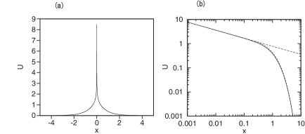
Figure 1: (a) A singular 1D soliton with $k=1$, produced by the numerical solution of Eq. (54). (b) The double-logarithmic plot of the same solution at small values of $x$ is presented by the solid curve. The dashed line is the analytical prediction provided by Eq. (7), and the dotted curve, which is almost indistinguishable from the solid one, is the approximation given by Eq. (9).

The stability of the entire family of the 1D singular solitons, suggested by the fact that it satisfies the conjectured aVK criterion, is fully confirmed by systematic simulations (the above-mentioned fixed boundary conditions at $x=\pm\Delta/2$ are essential for running the simulations). To illustrate this conclusion, results of the direct simulations are displayed in Figs. 2(a) and (b), for the solutions with $k=1$ and $k=0.5$. The numerical simulations of 1D equations (4) and (1) (with $g_{3}=g_{5}=0$) were performed in domain $|x|\leq 12.5$ with zero boundary conditions at $x=\pm 12.5$, using the split-step Fourier method based on a set of $16384$ modes,the respective mesh sizes being $\Delta x=25/16384\approx\allowbreak 1.526\times 10^{-3}$ and $\Delta z=10^{-6}$. At the central points, $x=\pm\Delta/2$, steadily oscillating boundary values

$$u(\pm\Delta/2)=\exp(ikz)U(\Delta/2)$$ (55)

are imposed, with $k=(3.1478/N)^{6}$ taken as per Eq. (10), $U(\Delta/2)$ being the value numerically evaluated by means of the RK method, as said above. The initial conditions are provided by the stationary singular solitons produced by the RK method. The profiles produced by the evolution are virtually indistinguishable from the input. Simulations with small random perturbations added to the input corroborate the stability.

Robustness of the singular solitons against large perturbations was tested by direct simulations of Eq. (1) with boundary conditions (55), with inputs strongly different from the stationary solitons corresponding to given $k$. As an example, Fig. 2(c) demonstrates the result for fixed $k=1$ in Eq. (55) with the mismatched input, taken as the stationary singular soliton corresponding to $k=0.5$, but with the amplitude rescaled so as to make the total norm equal to that corresponding to $k=1$. The result, produced by the simulations at $z=5$, is indistinguishable from the one displayed in Fig. 2(a), which was generated by the input in the form of the stationary soliton corresponding to the “correct” value, $k=1$.

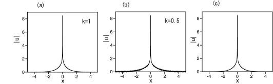
Figure 2: Snapshots of the 1D singular solitons, $|u(x,z)|$, at $z=5$, produced by direct simulations of Eq. (1), with the input taken as per the stationary solutions with $k=1$ (a) and $k=0.5$ (b). The solutions keep the same shape at $z>5$. (c) The snapshot of $|u\left(x,z=5\right)|$, produced by the simulation of Eq. (1) with boundary conditions (55) for $k=1$, initiated by the stationary solution for the singular soliton with $k=0.5$, see the text.

Finally, the comparison of the singular-soliton solution with that produced by the nonlinearity-screened attractive delta-functional potential, in the framework of Eq. (13), is displayed in Fig. 3. The ground-state solution of Eq. (13) was obtained by means of the imaginary-integration method, applied to the nonstationary version of Eq. (13). The approximate delta-function, $\tilde{\delta}$, was realized on the numerical mesh by setting $\tilde{\delta}=1/\left(4\Delta\right)$ at points $x=\pm 3\Delta/2$ and $\pm\Delta/2$, and $\tilde{\delta}=0$ elsewhere ($\Delta=25/16384\approx\allowbreak 1.526\times 10^{-3}$ and the domain’s definition, $|x|~{}\leq 12.5$, are the same as above). The comparison corroborates that the singular solitons can be realized as the ground state generated by the delta-functional potential screened by the septimal self-repulsion. Weak divergence of the comparison at very small values of $|x|$ and very large $\varepsilon$ is explained by the limited accuracy of the numerical scheme with a fixed mesh size, $\Delta$.

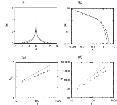
Figure 3: (a) The comparison of the singular-soliton solution from Fig. 1, shown by the long-dashed profile, with numerically generated ground-state solutions of Eq. (13) (see details in the text), for $\varepsilon=40$ and $400$ (the short-dashed and continuous profiles, respectively). (b) The same as in (a), but displayed in the double-logarithmic form. (c) The chain of rhombic symbols, connected by the short-dashed line as the guide to the eye, shows the peak amplitude of the numerically found solutions, $A_{p}\equiv U(x=\pm\Delta/2)$, vs. $\varepsilon$, while the long-dashed line shows the respective analytical approximation, $A_{p}=\left(\sqrt{2}\varepsilon\right)^{1/3}$, as given by Eqs. (14) and (15) with $x=0$. (d) The chain of symbols shows the dependence of the Hamiltonian of numerically generated solutions on $\varepsilon$, with the dashed line showing the respective analytical approximation, given by Eq. (17).

III.2 The 2D model

The existence and stability of fundamental ($S=0$) 2D singular solitons, produced by the quintic equation (18) with $\sigma=+1$ (self-repulsion), has been completely corroborated by numerical solutions of the equation. The mesh size $\Delta=25/2048\approx 1.221\times 10^{-2}$ was used in this case. Figure 4(a) displays the radial profile of the solution produced at $z=5$ by direct simulations of the radial version of Eq. (18),

$$i\frac{\partial u}{\partial z}=-\frac{1}{2}\left(\frac{\partial^{2}u}{\partial r^{2}}+\frac{1}{r}\frac{\partial u}{\partial r}\right)+|u|^{4}u,$$ (56)

with the input taken in the form of the exact analytical solution (22) corresponding to $k=0$. Panel 4(b) compares the numerical solution with the input at small values of $r$, confirming that Eq. (22) provides an asymptotically exact solution for $x\rightarrow 0$. Figure 4(c) displays the radial profile of the solution of Eq. (18) for $k=1$ at $z=5$. Panel 4(d) compares the numerical solution with analytical results given by Eqs. (22) and (25) with fitting constant $C=0.9$ (dashed and dotted lines, respectively).

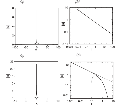
Figure 4: (a) Snapshot of solution $|u(r,z)|$ at $z=5$, produced by direct simulations of the 2D radial equation (56), which was initiated by the input taken as per the exact analytical solution for $k=0$, given by Eq. (22) (the solution is shown by the cross section along $y=0$). (b) The comparison of the numerical solution (the continuous line) with the input (the dashed line) at small values of $r$, on the double-logarithmic scale. The dashed line is the analytical expression (22). (c) The snapshot of solution $|u(r,z)|$ at $z=5$ for $k=1$, produced by direct simulations of the 2D radial equation (56). (d) The snapshot of the same solution, shown on the double-logarithmic scale. The long- and short-dashed lines represent, respectively, the analytical expressions given by Eqs. (22) and (25), with fitting parameter $C=0.9$.

Further, the full stability analysis of 2D solitons must include a possibility of azimuthal perturbations which break the axial symmetry of the solution, which makes it necessary to run simulations of the full 2D equation (18), in addition to the simulations of the radial equation ( 56). The result of the simulations, displayed in Fig. 5, clearly corroborates the stability of the 2D fundamental solitons against azimuthal perturbations.

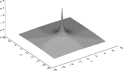
Figure 5: The same solution as in Fig. 4(c), but produced by simulation of the full 2D equation (18).

The above analytical consideration of the 2D singular solitons with embedded vorticity $S\geq 1$, which are solutions of Eq. (18) with $\sigma=-1$ (self-attraction), corresponding to the asymptotic form (23), has led to the conjecture that all the vortex solitons are unstable, as they do not satisfy the Vakhitov-Kolokolov criterion. This prediction is confirmed, in Fig. 6(a), by simulations of the radial reduction of Eq. (18) with $\sigma=-1$, for $S=1$:

$$i\frac{\partial u}{\partial z}=-\frac{1}{2}\left(\frac{\partial^{2}u}{\partial r^{2}}+\frac{1}{r}\frac{\partial u}{\partial r}-\frac{S^{2}}{r^{2}}u\right)-|u|^{4}u.$$ (57)

The simulations of Eq. (57) were performed with input

$$u_{0}(r)=(3/8)^{1/4}r^{-1/2},$$ (58)

taken as per Eq. (23) with $S=1$. The instability, which may signalize a transition to the supercritical collapse, driven by the quintic self-attraction in 2D, is clearly seen in Fig. 6(a). Similar instability was found for other values of $S\neq 0$. In fact, splitting instability of the vortex states is expected to develop still faster in the framework of the full 2D equation (18).

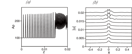
Figure 6: (a) The evolution of the peak amplitude, $A_{p}$, of solution $|u(x,y,z)|$ [i.e., values of $\left|u\left(x,y=\pm\Delta/2\right)\right|$, see Eq. (53)], as produced by simulations of Eq. (57) with the quintic self-attraction, for a 2D singular soliton with embedded vorticity $S=1$. The input is taken as per Eq. (58). (b) The evolution of the radial profiles, $\left|u(r,z)\right|$, for the same solution. Numbers attached to the vertical axis indicate values if $z$ in the course of the evolution.

III.3 The 3D model

Numerical solutions of the 3D model were performed with the mesh size $\Delta=5/4096\approx\allowbreak 1.221\times 10^{-3}$. Radial profiles of 3D isotropic singular solitons were found as solutions of Eq. (33). Formal comparison of these solutions to the analytical prediction, given by Eq. (34) for $r\rightarrow 0$, is not straightforward, as the latter expression contains a slowly varying logarithmic factor, which depends on indefinite parameter $r_{0}$. Therefore, the comparison at small values of $r$ was performed with analytical profile $\mathrm{const}\cdot r^{-1}$, where the constant was selected as the best-fit parameter. An example is displayed in Fig. 7 (a), where analytical fits for the comparison with the numerically found solution pertaining to $k=1$ are chosen, at small and large $r$, as $0.001\cdot r^{-1}$ and $0.001\exp(-\sqrt{2}r)\cdot r^{-1}$, respectively, the latter one corresponding to Eq. (35). It is seen that the fit provides asymptotically exact agreement.

Finally, the stability of the 3D singular solitons was verified by direct simulations of the radial version of Eq. (32),

$$i\frac{\partial u}{\partial t}=-\frac{1}{2}\left(\frac{\partial^{2}u}{\partial r^{2}}+\frac{2}{r}\frac{\partial u}{\partial r}\right)+|u|^{2}u=0,$$ (59)

with the initial condition taken as the stationary solution, such as the one shown in Fig. 7(a). An example displayed in Fig. 7(b) confirms that the 3D singular solitons are stable states.

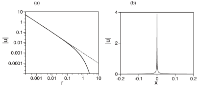
Figure 7: (a) The comparison, on the double-logarithmic scale, of the numerically obtained stationary solution of Eq. (33) with $\omega=-1$ (the continuous line) with the semi-analytical profiles, $0.001\cdot r^{-1}$ (the long-dashed line) and $0.001\exp(-\sqrt{2}r)/r$ (the short-dashed line), see the text. The difference between the numerical solution and the latter analytical approximation is hardly visible. (b) The radial cross section of the 3D isotropic singular soliton, produced at $z=2$ by direct simulations of Eq. (59), with the initial taken configuration taken from panel (a).

IV Conclusion

The objective of the present work is to demonstrate that the traditional concept of solitons as regular self-trapped solutions, supported by the competition of self-focusing nonlinearity and linear dispersion or diffraction, may be extended to singular solutions with a convergent norm. These singular states are supported by a purely defocusing nonlinearity, provided that it is strong enough, viz., septimal, quintic, and usual cubic terms, in the 1D, 2D, and 3D settings, respectively (the possibility of such singularities, produced by the stationary 1D and 2D equations, was first reported in Ref. Veron1 ). Such counter-intuitive solutions may be naturally interpreted as describing a result of complete screening of a delta-functional attractive potential by the repulsive nonlinearity, the respective “charge” (full strength of the attractive potential) being infinite in 1D, finite in 2D, and vanishing in 3D. The required septimal and quintic self-repulsive nonlinearity can be realized in planar and bulk colloidal waveguides for light beams, while the 3D equation with the cubic self-repulsion is the usual GPE (Gross-Pitaevskii equation) for BEC. The realization of the singular solitons in terms of the screened delta-functional attractive potential suggests a possibility of their experimental creation. In particular, a narrow stripe carrying a high value of the refractive index, embedded in a planar solid-colloidal planar waveguide, may be used for the making of the effectively 1D soliton. The comparison with numerical results confirms that the analytical results provide accurate approximations for the singular solitons at small and large distances from the origin. Stability of the singular states is exactly predicted by the conjectured aVK (anti-Vakhitov-Kolokolov) criterion. In addition to the fundamental solitons, the 2D model with the quintic self-attraction admits singular solitons with embedded vorticity, but they are completely unstable. The possibility of the existence of relevant solutions in the form of dissipative singular solitons, in the 1D, 2D, and 3D models with a complex coefficient in front of the nonlinear term, is briefly considered too.

As an extension of the present analysis, it may be relevant to consider interactions between stable singular solitons.

References

- (1) M. Quiroga-Teixeiro and H. Michinel, Stable azimuthal stationary state in quintic nonlinear optical media, J. Opt. Soc. Am. B 14, 2004-2009 (1997).
- (2) R. L. Pego and H. A. Warchall, J. Nonlinear Sci. 12, 347 (2002).
- (3) D. Mihalache, D. Mazilu, I. Towers, B.A. Malomed, F. Lederer, J. Optics A 4, 615 (2002).
- (4) D. Mihalache, D. Mazilu, B.A. Malomed, F. Lederer, J. Opt. B 6, S341 (2004).
- (5) D. Mihalache, D. Mazilu, L.-C. Crasovan, I. Towers, A. V. Buryak, B. A. Malomed, L. Torner, J. P. Torres, and F. Lederer, Phys. Rev. Lett. 88, 073902 (2002).
- (6) D. Mihalache, D. Mazilu, L.-C. Crasovan, I. Towers, B. A. Malomed, A. V. Buryak, L. Torner, and F. Lederer, Phys. Rev. E 66, 016613 (2002).
- (7) B. A. Malomed, Physica D 339, 108 (2019).
- (8) D. Mihalache, D. Mazilu, L.-C. Crasovan, B. A. Malomed, F. Lederer, and L. Torner, J. Optics B 6, S333 (2004).
- (9) D. S. Petrov, Phys. Rev. Lett. 115, 155302 (2015).
- (10) D. S. Petrov and G. E. Astrakharchik, Phys. Rev. Lett 117, 100401 (2016).
- (11) C. R. Cabrera, L. Tanzi, J. Sanz, B. Naylor, P. Thomas, P. Cheiney, L. Tarruell, Science 359, 301 (2018).
- (12) P. Cheiney, C. R. Cabrera, J. Sanz, B. Naylor, L. Tanzi, and L. Tarruell, Phys. Rev. Lett. 120, 135301 (2018).
- (13) C. D’Errico, A. Burchianti, M. Prevedelli, L. Salasnich, F. Ancilotto, M. Modugno, F. Minardi, and C. Fort, arXiv:1908.00761.
- (14) G. Semeghini, G. Ferioli, L. Masi, C. Mazzinghi, L. Wolswijk, F. Minardi, M. Modugno, G. Modugno, M. Inguscio, and M. Fattori, Phys. Rev. Lett. 120, 235301 (2018).
- (15) G. Ferioli, G. Semeghini, L. Masi, G. Giusti, G. Modugno, M. Inguscio, A. Gallemi , A. Recati, and M. Fattori, Phys. Rev. Lett. 122, 090401 (2019).
- (16) G. E. Astrakharchik and B. A. Malomed, Phys. Rev. A 98, 013631 (2018).
- (17) Y. V. Kartashov, B. A. Malomed, L. Tarruell, and L. Torner, Phys. Rev. A 98, 013612 (2018).
- (18) Y. V. Kartashov, B. A. Malomed, and L. Torner, Phys. Rev. Lett. 122, 193902 (2019).
- (19) Y. Li, Z. Chen, Z. Luo, C. Huang, H. Tan, W. Pang, and B. A. Malomed, Phys. Rev. A 98, 063602 (2018).
- (20) E. L. Falcão-Filho, C. B. de Araújo, G. Boudebs, H. Leblond, and V. Skarka, Phys. Rev. Lett. 110, 013901 (2013).
- (21) A. S. Reyna, G. Boudebs, B. A. Malomed, and C. B. de Araújo, Phys. Rev. A 93, 013840 (2016).
- (22) A. S. Reyna and C. B. de Araújo, Opt. Exp. 22, 22456 (2014).
- (23) A. S. Reyna and C. B. de Araújo, Adv. Opt. Phot. 9, 720 (2017).
- (24) A. S. Reyna, K. C. Jorge, and C. B. de Araújo, Phys. Rev. A 90, 063835 (2014).
- (25) A. S. Reyna, B. A. Malomed, and C. B. de Araújo, Phys. Rev. A 92, 033810 (2015).
- (26) Y. S. Kivshar and G. P. Agrawal, Optical Solitons: From Fibers to Photonic Crystals (Academic Press: San Diego, 2003).
- (27) T. Dauxois and M. Peyrard, Physics of Solitons (Cambridge University Press: Cambridge, 2006).
- (28) J. Yang, Nonlinear Waves in Integrable and Nonintegrable Systems (SIAM: Philadelphia, 2010).
-
(29)
H. Sakaguchi and B. A. Malomed. Phys. Rev. A 81,
013624 (2010).
- (30) L. Veron, Nonlinear Analysis, Theory. Methods & Applications 5, 225 (1981).
- (31) H. Brezis and L. Veron, Archive for Rational Mechanics and Analysis 75, 1 (1980).
- (32) O. V. Borovkova, Y. V. Kartashov, L. Torner, and B. A. Malomed, Phys. Rev. E 84, 035602 (2011).
- (33) Y. V. Kartashov, B. A. Malomed, Y. Shnir, and L. Torner, Phys. Rev. Lett. 113, 264101 (2014).
- (34) R. P. Feynman, Quantum Electrodynamics (Westview Press: 1998).
- (35) H. Sakaguchi and B. A. Malomed, Phys. Rev. A 84, 033616 (2011).
- (36) L. Bergé, Phys. Rep. 303, 259-370 (1998).
- (37) G. Fibich, The Nonlinear Schrödinger Equation: Singular Solutions and Optical Collapse (Springer: Heidelberg, 2015).
- (38) N. G. Vakhitov and A. A. Kolokolov, Radiophys. Quantum Electron. 16, 783 (1973).
- (39) Y. Kartashov, G. Astrakharchik, B. Malomed, and L. Torner, Nature Reviews Physics 1, 185 (2019).
- (40) M. A. Porras, A. Parola, D. Faccio, A. Dubietis, and P. Di Trapani, Phys. Rev. Lett. 93, 153902 (2004).
- (41) M. J. Ablowitz and Z. H. Musslimani, Phys. Rev. Lett. 110, 064105 (2013).