The Cluster Ages Experiment (CASE). VIII. Age and Distance of the Globular Cluster 47 Tuc from the Analysis of Two Detached Eclipsing Binaries

Abstract

We use photometric and spectroscopic observations of the eclipsing binary E32 in the globular cluster 47 Tuc to derive the masses, radii, and luminosities of the component stars. The system has an orbital period of 40.9d, a markedly eccentric orbit with $e=0.24$, and is shown to be a member of or a recent escaper from the cluster. We obtain $M_{p}=0.862\pm 0.005M_{\odot}$, $R_{p}=1.183\pm 0.003R_{\odot}$, $L_{p}=1.65\pm 0.05L_{\odot}$ for the primary and $M_{s}=0.827\pm 0.005M_{\odot}$, $R_{s}=1.004\pm 0.004R_{\odot}$, $L_{s}=1.14\pm 0.04L_{\odot}$ for the secondary. Based on these data and on an earlier analysis of the binary V69 in 47 Tuc we measure the distance to the cluster from the distance moduli of the component stars, and, independently, from a color - surface brightness calibration. We obtain 4.55$\pm$0.03 and 4.50$\pm$0.07 kpc, respectively – values compatible within 1$\,\sigma$ with recent estimates based on $Gaia$ DR2 parallaxes. By comparing the $M-R$ diagram of the two binaries and the color-magnitude diagram of 47 Tuc to Dartmouth model isochrones we estimate the age of the cluster to be $12.0\pm 0.5$ Gyr, and the helium abundance of the cluster to be Y$\approx$0.25.

1 Introduction

The Cluster AgeS Experiment (CASE) is a project devoted to the study of detached eclipsing binaries (DEBs) in nearby globular clusters (GCs). In the preceding papers of this series we have shown that masses, luminosities and radii of DEB components on the cluster main sequence (MS) or subgiant branch (SG) can be derived with a precision of better than 1%. This, in turn, allows a determination of GC ages and distances independently of color-magnitude diagram (CMD) fitting, and for tests of evolution models of metal-poor stars. The methods and assumptions we employ follow the ideas of Paczyński (1997) and Thompson et al. (2001); more details can be found in Kaluzny et al. (2002). Thus far, we have presented results for eight binaries with MS or SG components in four GCs: 47 Tuc (Thompson et al., 2010, hereafter TK10), M4 (Kaluzny et al., 2013b), M55 (Kaluzny et al., 2014) and NGC 6362 (Kaluzny et al., 2015). These are the first and, to the best of our knowledge, the only direct measurements of the fundamental parameters of such stars in GCs.

Based on the analysis of the turnoff binary V69, Dotter et al. (2009, hereafter D9) and TK10 performed an age and distance study of 47 Tuc, which has recently been repeated by Brogaard et al. (2017, hereafter B17) using independent photometric data. The present paper extends the study by including a second DEB, discovered by Kaluzny et al. (2013a), and henceforth referred to as E32. Like V69, E32 resides at the turnoff of 47 Tuc, however its secondary is in a markedly less advanced evolutionary state than that of V69, thus providing an excellent additional anchor point for isochrone fitting. Moreover, supplementary IR observations performed at the maximum light of both systems have permitted a significant reduction of the temperature errors compared to those of TK10, and an updated velocity curve of V69 has enabled a reduction of the uncertainties in the component masses by $\sim$30%.

This paper is based on photometric and spectroscopic observations described in Section 2. Section 3 (together with Appendix A) is devoted to a period analysis of E32, and in Section 4 the parameters of the binary are derived. In Section 5 we argue that E32 is a member of or a recent escaper from the cluster. An age and distance analysis of 47 Tuc is presented in Section 6, and the results are summarized and discussed in Section 7.

2 Observational material and data reduction

2.1 Spectroscopy

The velocity curve of E32 is based on echelle spectra obtained between UT July 13th, 2013 and UT July 9th, 2015 with the MIKE spectrograph (Bernstein et al., 2004) on the Magellan-Clay telescope and with the UVES spectrograph on the ESO VLT Kueyen telescope. Additional observations of V69 were obtained with the MIKE spectrograph between UT July 1, 2008 and UT July 8, 2014.

2.1.1 UVES Spectroscopy of E32

UVES spectra of E32 were taken using the red arm of the instrument, with a 0.8 arcsec slit providing a resolution of R $\simeq$ 50,000. The acquisition of a single spectrum comprised two exposures lasting 1430 s each, followed by a single calibration exposure of a thorium-argon lamp. The observations were reduced with the ESO-UVES pipeline. In total, 16 spectra of E32 were obtained. Post extraction processing of the spectra was done with the IRAF-ECHELLE package.

2.1.2 MIKE Spectroscopy of E32 and V69

MIKE spectra of E32 and V69 were taken with the same instrument setup as outlined in TK10. The spectra were reduced with the procedures outlined in that paper. A total of 18 spectra of E32 and 22 spectra of V69 were obtained.

2.1.3 Velocity Measurements

Velocities of the components of E32 and V69 were determined following the methodology presented by TK10. The velocities were measured with the TODCOR algorithm (Zucker & Mazeh, 1994) using an implementation written by G. Torres. The same templates used in the TK10 study of V69 were used. These were synthetic spectra interpolated from the grid of Coelho et al. (2005) at ($\log g$, $T_{eff}$, and [Fe/H]) = (4.14, 5945 K, -0.71) for the primary and (4.24, 5955 K, -0.71) for the secondary. The measured velocities are insensitive to minor changes in these parameters. For each UVES observation of E32, velocities were measured on the wavelength intervals 4000 Å $<\lambda<$ 4300 Å and 4360 Å$<\lambda<$ 4600 Å, and then averaged to provide a final velocity. For each MIKE observation of E32 and V69, velocities were measured on the wavelength intervals 4125 Å$<\lambda<$ 4320 Å, 4350 Å$<\lambda<$ 4600 Å, and 4600 Å$<\lambda<$ 4850 Å, and then averaged to provide a final velocity.

The results for E32 are presented in Table 1 which lists Heliocentric Julian Dates (HJD-2450000) at mid-exposure, velocities of the primary and secondary components, and orbital phases of the observations.

As detailed in Section 3, processing of the light curves of E32 required an approximate ephemeris based on a preliminary orbital solution. To that end, the radial velocities from Table 1 were fitted with a non-linear least-squares solution using code written by T. Mazeh and G. Torres, with the MIKE and UVES velocities given equal weight in the fitting procedure. The UVES velocities were offset by +0.93 km s^-1 during the orbital fitting to minimize the overall standard deviation of the fits. The resulting preliminary orbital solution is presented in Table 2. The mean error of the velocities, estimated from the final fit to the photometric and spectroscopic data (see Fig 1 and Section 4.3), is $\pm$0.38 km s^-1.

The results for V69 are presented in Table 3. The orbit was solved for using the same code as for E32, adopting the ephemeris of TK10. The resulting orbit is presented in Table 4 and Figure 2. Since we have not added any new eclipse photometry we have only used the new radial velocity observations to improve upon the mass determinations of the components of V69 using the light curve solution of TK10 (their Table 5). The final masses for the components of V69 are $M_{p}\ =0.8750\pm 0.0043M_{\odot}$ and $M_{s}\ =0.8584\pm 0.0042M_{\odot}$.

Table 1: Heliocentric radial velocities of the components of E32.

HJD-2450000	$v_{\rm p}$ (km s-1)	$v_{\rm s}$ (km s-1)	Instrument	Phase*
6486.78206	-32.22	-49.51	MIKE	0.438
6490.87600	-46.31	-34.13	MIKE	0.538
6491.82881	-49.93	-30.11	MIKE	0.561
6518.78220	-4.71	-76.84	MIKE	0.220
6519.77841	-6.48	-75.07	MIKE	0.244
6521.78686	-11.96	-70.15	MIKE	0.293
6578.62743	-65.94	-13.42	MIKE	0.683
6579.58417	-68.99	-10.77	MIKE	0.706
6582.67235	-75.35	-2.60	MIKE	0.782
6583.61281	-77.17	-2.02	MIKE	0.805
6584.59316	-76.43	-0.86	MIKE	0.829
6585.60637	-76.99	-2.58	MIKE	0.853
6844.88429	-3.22	-78.69	MIKE	0.191
6845.86441	-4.47	-77.78	MIKE	0.215
6846.86186	-6.47	-75.97	MIKE	0.239
6851.85080	-21.28	-61.78	UVES	0.361
6872.78660	-75.45	-4.56	UVES	0.873
6882.66643	-6.45	-74.40	UVES	0.114
6882.72578	-6.19	-74.89	UVES	0.116
6884.74632	-2.69	-79.15	UVES	0.165
6885.69203	-2.99	-78.53	UVES	0.188
6887.78663	-5.94	-75.85	UVES	0.239
6901.63211	-51.95	-28.40	UVES	0.578
6901.67068	-52.04	-28.07	UVES	0.579
6902.87926	-55.97	-23.20	UVES	0.608
6903.57488	-58.77	-20.98	UVES	0.625
6906.66166	-68.29	-11.53	UVES	0.701
6906.75787	-68.35	-10.42	UVES	0.703
6922.64573	-11.10	-71.34	UVES	0.091
6923.69826	-6.87	-75.61	UVES	0.117
6925.56888	-2.89	-78.69	UVES	0.163
7210.86790	-4.17	-77.76	MIKE	0.136
7211.87558	-3.25	-79.02	MIKE	0.161
7212.89462	-3.13	-78.96	MIKE	0.186
*Ephemeris from Equation (1) derived in Section 3.

Table 2: Preliminary orbital parameters of E32.

Parameter	Value
$P$ (d)	40.9132(40)
$T_{0}$ (HJD-2450000)	6796.214(54)
$\gamma$ (km s-1)	-40.25(5)
$K_{p}$ (km s-1)	37.08(9)
$K_{s}$ (km s-1)	38.65(9)
$q$	0.9595(31)
$e$	0.2403(19)
$\omega$ (deg)	270.90(46)

Figure 1: Velocity curve of E32. Observational measurements are phased with the final ephemeris Equation (1) and compared to the final model derived in Section 4.3. Filled symbols represent data for the primary and open symbols are for the secondary. The systemic velocity is equal to $-40.25\pm 0.05$ km s^-1 and the RMS residuals are 0.34 km s^-1 for the primary and 0.40 km s^-1 for the secondary. Phase 0 corresponds to the center of the main (deeper) photometric minimum.

Table 3: New heliocentric radial velocities of the components of V69.

HJD-2450000	$v_{\rm p}$ (km s-1)	$v_{\rm s}$ (km s-1)	Phase*
4648.90500	21.73	-56.33	0.768
4649.89328	19.81	-54.38	0.802
4783.50899	-50.96	17.88	0.325
4784.55132	-44.27	11.15	0.360
5131.59025	-47.19	13.12	0.108
5132.59245	-53.62	19.41	0.142
5388.89247	18.05	-52.97	0.819
5389.84629	13.97	-48.80	0.851
5457.63885	-53.50	20.64	0.146
5458.68400	-58.15	24.82	0.181
5459.67316	-59.79	26.68	0.215
5770.77939	22.09	-56.63	0.747
5836.58836	-11.79	-21.07	0.975
6489.79307	-42.34	8.37	0.087
6490.84490	-49.88	16.29	0.123
6491.77732	-54.66	21.95	0.154
6578.66648	-44.37	11.86	0.096
6579.54487	-50.67	18.06	0.126
6580.53542	-55.45	23.23	0.159
6844.80654	-45.22	12.36	0.105
6845.78624	-51.52	18.62	0.139
6846.78443	-56.22	23.76	0.172
*Adopting the ephemeris from Table 4.

Table 4: Revised orbital parameters of V69.

Parameter	Value
$P$ (d)	29.53975*
$T_{0}$ (HJD-2450000)	53237.8421*
$\gamma$ (km s-1)	-16.79(5)
$K_{p}$ (km s-1)	41.04(9)
$K_{s}$ (km s-1)	41.83(9)
$q$	0.9811(29)
$e$	0.0558(9)
$\omega$ (deg)	150.72(172)
*Adopting the ephemeris of TK10.

Figure 2: Revised velocity curve of V69. Observational measurements are phased with the ephemeris given in Table (4). Filled symbols represent data for the primary and open symbols are for the secondary. The RMS residuals are 0.47 km s^-1 for the primary and 0.43 km s^-1 the secondary. Phase 0 corresponds to the center of the main (deeper) photometric minimum.

2.2 Photometry

Our photometric data comprise four sets of measurements, spanning the period from May 2010 to January 2018, and identified in Table 5. OGLE observations were processed by the standard OGLE pipeline (Udalski, Szymański & Szymański, 2015), yielding $V_{\mathrm{m,O}}=17.079$ mag and $I_{\mathrm{m}}=16.383$ mag at the maximum light of the system, with errors dominated by the zero-point uncertainty of 0.02 mag. The photometry of du Pont frames was performed using an image subtraction technique implemented in the DIAPL package. Differential counts were converted to magnitudes based on profile photometry and aperture corrections extracted from reference images with the help of standard DAOPHOT, ALLSTAR and DAOGROW packages (Stetson, 1987, 1990). Instrumental magnitudes were transformed to the $BV$ system using stars from the color-magnitude diagram of Kaluzny et al. (2013a) as secondary standards. At the maximum light we obtained $V_{\mathrm{m,C}}=17.117$ mag and $B-V=0.561$ with errors dominated by the 0.011 mag uncertainty of the offset term. Since the zero-point uncertainty of Kaluzny et al. (2013a) photometry is 0.01 mag, the total error of our photometry may be estimated at 0.015 mag.

CASE and OGLE $V$-band data were combined into a single light curve, and the offset between the two photometric systems was accounted for by adopting the weighted mean of $V_{\mathrm{m,C}}$ and $V_{\mathrm{m,O}}$ as the $V$-band magnitude at maximum light which is listed in Table 6 together with the colors of E32. The reduced light curves phased with the ephemeris derived in Section 3 are plotted in Fig. 3, and Fig. 4 shows the $O-C$ residuals from the final fit derived in Section 4.3. The $RMS$ residuals are equal to 12.6, 9.8 and 11.4 mmag for $B$, $V$ and $I$ filters, respectively. We note that the colors of E32 are nearly constant during the eclipses, indicating nearly equal temperatures of the components.

The optical data were supplemented by single IR frames taken on UT December 10th, 2013 in $J$ and $K_{s}$ bands with the FourStar camera on the Magellan Baade telescope (Persson et al., 2013). Both E32 and V69 were then at maximum light (phases 0.89 and 0.63, respectively). Four pointings were used in a 2x2 grid to tile over the cluster. At each pointing images were taken in a five-point "rotated-dice" dither pattern to cover the gaps between the four detectors. Two exposures of 11.644 seconds each were taken at each pointing for a total effective exposure of 116.44 seconds over the central 20x20 arcminutes of the cluster. The raw images were linearized, flat-fielded and then background subtracted using sparse frames which were masked of sources and averaged together. The processed images were then distortion corrected, aligned and co-added to make a mosaic 9000$\times$9000 px image of the cluster.

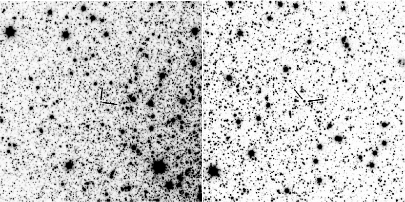
Figure 11: Charts of E32 (left) and V69 fields used to calibrate the FourStar photometry. Each chart is 2′on a side, with north to the top and east to the left. The original frames were taken with the FourStar camera in the $K_{\mathrm{s}}$ band.

For the calibration of IR observations data from the 2MASS catalog (Skrutskie et al., 2006) were used. Since our IR frames were stitched from several FourStar images, we decided to independently calibrate 740$\times$740 px subfields centered on E32 and V69, and shown in Fig. 11. Standard DAOPHOT, ALLSTAR, and DAOGROW packages (Stetson, 1987, 1990) were applied to extract the profile photometry from each subfield, and 2MASS counterparts of FourStar objects were identified. 2MASS blends, stars with undetermined 2MASS photometry errors, and stars overexposed in FourStar frames were rejected. Outliers of $\Delta J$ and $\Delta K_{\mathrm{s}}$ differences between 2MASS and FourStar magnitudes were eliminated by 2$\sigma$-clipping, leaving 24, 26, 20, and 29 stars, respectively, in E32 $J$, V69 $J$, E32 $K_{\mathrm{s}}$, and V69 $K_{\mathrm{s}}$ subfield. The respective offsets were calculated as error-weighted means of $\Delta J$ and $\Delta K_{\mathrm{s}}$, yielding
$J^{2\mathrm{M}}=J^{4\mathrm{S}}$ + 1.882(18) mag,
$J^{2\mathrm{M}}=J^{4\mathrm{S}}$ + 2.032(13) mag,
$K_{\mathrm{s}}^{2\mathrm{M}}=K_{\mathrm{s}}^{4\mathrm{S}}$ + 0.971(22) mag,
$K_{\mathrm{s}}^{2\mathrm{M}}=K_{\mathrm{s}}^{4\mathrm{S}}$ + 1.018(20) mag
with no detectable dependence on the color; 2M and 4S standing for 2MASS and FourStar. The large difference between $\Delta J$ offsets is perplexing, but we are sure we made no mistake here. Moreover, we suspect that the $J$-offset for E32 subfield should be even smaller, as the temperatures of E32 components calculated from $(V-J)_{0}$ are by over 150 K higher than those calculated from the remaining indices (see Section 4.4). To remain on the safe side, we decided to used the $J$-band data solely for transforming $V-K_{\mathrm{s}}$ into Johnson $V-K$ (see Section 6.1).

Table 5: Light curves used for modeling of E32.

Filter	Telescope	1st day	last day	Number of
		[HJD-2450000]		data points
B	du Pont	7634	8125	409
V	du Pont	7634	8125	957
V	OGLE	5391	8043	304
I	OGLE	5346	8126	797

Table 6: $BVIJK_{\mathrm{s}}$ photometry of E32 and V69 at maximum light

	$V$	$B-V$	$V-I$	$V-J$	$V-K_{\mathrm{s}}$
E32	17.103(15)	0.561(21)	0.696(25)	1.084(025)	1.495(29)	(mag)
V69	16.836(01)*	0.548(02)*		1.147(025)	1.534(28)	(mag)
*From TK10.

Figure 3: E32 light curves used in this paper (see Table 5 for the list), phased with the final ephemeris (1).

Figure 4: $IVB$ residuals of the fits to the light curves for the primary (top) and secondary minimum (bottom). For clarity, $I$ and $V$ residuals are offset by 0.2 and 0.1 mag, respectively.

3 Period determination

With a long orbital period almost equal to an integer number of days, and eclipses lasting over seven hours, a well sampled eclipse light curve of E32 is difficult to obtain. As a result the $V$-band observations yielded no unique ephemeris. To get the best possible coverage, we decided to combine all accessible data in $V$, $B$, and $I$ filters into a single light curve. The analysis of the combined data, detailed in Appendix A, yielded the following ephemeris:

$$\begin{split}T_{min}&=2457246.21655(20)+40.912883(13)\times E\\ &+II_{min}\times 20.3311(9),\end{split}$$ (1)

where $II_{min}$ = 0 or 1 for primary and secondary eclipses, respectively. The epoch closest to the median observation time was selected to minimize the correlation of errors of $T_{0}$ and $P$.

4 Data analysis and system parameters

4.1 Techniques and basic assumptions

The data were analyzed with the JKTEBOP v.34 code which can fit radial velocities simultaneously with a light curve (Southworth, 2013, and references therein), and is capable of a robust search for the global minimum in the parameter space. Because of significantly smaller number of points and poorer coverage of the minima in the $B$ and $I$-bands, only the $V$-band light curve was used for the final photometric solution. The $B$ and $I$ fits were performed with all parameters taken from the $V$-band fit and fixed except the light scaling factor and the central surface brightness ratio $s$. These served exclusively to calculate contributions of the system components to the total light, from which component magnitudes and color indices were obtained.

Since E32 is a very well detached system (see Fig. 3), reflection effects were neglected. The gravity darkening coefficient was set to $g=0.32$, a value appropriate for stars with convective envelopes. For the present analysis to be compatible with that of TK10, we assumed a square-root law for the limb darkening with coefficients interpolated from the tables of Claret (2000) using the jktld code, and adopting [Fe/H] = $-0.71$ together with an $\alpha$-element enhancement of +0.4.

In the du Pont frames E32 is well separated from its three closest neighbors, and in HST frames (for example, the ACS/WFC frame J8CDD1F0Q; Proposal 9028, P.I. G. Meurer) we did not find any evidence for the system being an unresolved blend. Also, we found no evidence of a third component in the cross-correlations of the spectra. We therefore assumed that the light curves of E32 are not contaminated by any “third light” effects.

4.2 Lifting the degeneracy

Despite an appreciably flattened orbit (see Fig. 1), the secondary eclipse in E32 occurs at a phase of nearly 0.5, which means that we must be looking at the binary almost along the major axis. Moreover, since the temperatures of the components are nearly the same (see Section 2.2), the difference in depths of the minima must originate mainly from the geometrical effect. Such a combination of parameters results in a strong degeneracy of the solutions in the sense that fits with significantly differing component radii are equally acceptable given the observational errors.

To illustrate this effect quantitatively we fitted the $V$-light curve for several fixed values $89\leq i\leq 89.07$, iterating for all the remaining parameters. For the central surface brightness ratio, $s$, and the radii of the primary and secondary we obtained ranges $0.925\leq s\leq 0.985$ and $1.020\leq r_{p}\leq 1.247R_{\odot}$ and $0.908\leq r_{s}\leq 1.190R_{\odot}$ while the residuals $\sigma_{\mathrm{O-C}}$ varied between 9.82 and 9.87 mmag. Since these large uncertainties make $r_{p}$ and $r_{s}$ practically useless for isochrone fitting, the degeneracy had to be lifted.

To that end we utilized the information contained in the spectra of E32, employing a procedure described in Rozyczka et al. (2014). Briefly, using the library of Coelho et al. (2005) we calculated synthetic spectra of the system for $\log g=4.0$ and $\log g=4.5$ (i.e. values bracketing those found by TK10), with $T_{\mathrm{eff}}$ estimated from dereddened $B-V$ and $V-I$ colors of the system, taking $E(B-V)=0.04$ and $E(V-I)=0.06$ from TK10. The empirical calibration of (Casagrande et al., 2010, hereafter C10) yielded $T_{\mathrm{eff}}=6012\pm 73$ K and $T_{\mathrm{eff}}=6007\pm 59$ K, respectively for the two indices. For the further analysis a rounded value of $T_{\mathrm{eff}}=6000$ K was adopted.

The spectra retrieved from the library were Doppler-shifted to geocentric component velocities. Since we found that there was practically no difference between spectra with $\log g=4.0$ and $\log g=4.5$, calculations were continued for $\log g=4.5$ only. Rotational broadening was not applied, as a broadening-function analysis (Kaluzny et al., 2006, and references therein) yielded negligible rotational velocities of the order of 2–3 km s^-1, consistent with the adopted gravity darkening The derived pairs of spectra, each corresponding to a given phase, were then combined in various proportions and compared with the observed spectrum taken at the same phase.

Only MIKE spectra were used for the comparison, as their S/N was better than for the UVES data. The comparison itself was performed separately for five different spectral segments between 4085 Å and 4845 Å, each 30 Å long except the 50 Å long segment beginning at 4280 $\AA$ (short segments of the spectra were compared rather than the whole available range in order to account for the varying mean intensity). For each phase and each segment the best value of the total secondary-to-primary light ratio $l_{r}$ was found by minimizing $\sigma_{\mathrm{O-C}}$. The mean of all of the measured light ratios, $l_{r}=0.69\pm 0.06$, was used for further analysis. We note that Rozyczka et al. (2014) reached a significantly better accuracy $(l_{r}=0.707\pm 0.024)$ in an analysis of the DEB V15 in the metal-rich open cluster NGC 6253; however their spectra had a much larger S/N ratio simply because V15 is 2.3 mag brighter than E32.

4.3 Final model fitting

Since $l_{r}$ is an $output$ parameter of JKTEBOP, the search for models meeting the condition $l_{r}=0.69\pm 0.06$ had to be performed implicitly. We defined grids $89.01\leq i_{k}\leq 89.97$ and $0.925\leq s_{j}\leq 0.985$, and fitted models for all pairs $(i_{k},s_{j})$ with both $i_{k}$ and $s_{j}$ kept fixed while fitting. Among fits with $l_{r}=0.69\pm 0.06$ we found only one minimum of $\sigma_{\mathrm{O-C}}$, reached for $(89.025,0.9352)$ and yielding $l_{r}=0.680$. The model corresponding to that minimum was adopted as the final solution with errors estimated using a modified Monte Carlo option of JKTEBOP (namely, for each perturbed set of observational data the entire procedure of searching for a minimum of $\sigma_{\mathrm{O-C}}$ was repeated). The parameters of E32 derived from this final photometric solution are given in Table 7.

Table 7: Final model of E32.

Parameter	Value
$P$ (d)	40.912883(13)
$A\;(R_{\odot})$	59.46(10)
$e$	0.2428(10)
$\omega$ (deg)	271.044(9)
$M_{p}\;(M_{\odot})$	0.8617(47)
$M_{s}\;(M_{\odot})$	0.8268(45)
$R_{p}\;(R_{\odot})$	1.1834(34)
$R_{s}\;(R_{\odot})$	1.0045(40)
$L_{s,B}/L_{p,B}$	0.669(11)
$L_{s,V}/L_{p,V}$	0.680(6)
$L_{s,I}/L_{p,I}$	0.693(9)

Table 8: Magnitudes and colors of the components of E32 and V69.

Star	Filter/color	primary	secondary
		(mag)	(mag)
E32	$V$	17.666(15)	18.085(16)
E32	$B-V$	0.554(23)	0.572(24)
E32	$V-I$	0.688(27)	0.708(28)
E32	$V-J$	1.073(26)	1.100(27)
E32	$V-K_{\mathrm{s}}$	1.479(30)	1.518(30)
V69∗	$V$	17.468(10)	17.724(10)
V69∗	$B-V$	0.551(14)	0.544(14)
V69	$V-J$	1.152(27)	1.140(28)
V69	$V-K_{\mathrm{s}}$	1.542(29)	1.524(30)
∗From TK10.

Using data from Tables 6 and 7, $BVI$ magnitudes and colors of the components of E32 were derived. These are given in Table 8 together with $BV$ data derived for V69 by TK10. For completeness, Table 8 also lists the $JK_{\mathrm{s}}$ photometry for which the light ratios are obtained in Section 4.4.

As demonstrated in the color-magnitude diagram (Fig. 5), the components of V69 and E32 are located on the main sequence close to the turnoff point, with the secondary of E32 significantly extending the luminosity range available for isochrone fitting. A systematic effect in the color uncertainty of ground-based observations is illustrated by the difference between positions of V69 system derived by TK10 and, from independent photometric data, by B17.

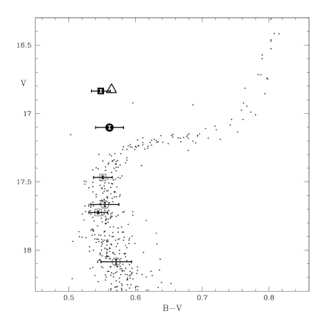
Figure 5: Positions of V69 (after TK10; squares) and E32 (circles) in the CMD of 47 Tuc. Open and filled symbols indicate, respectively, individual components and combined light of each system. The background stars are the same as in Fig. 4. of TK10. Triangle marks the position of V69 system derived by B17.

4.4 Temperatures and luminosities

As discussed by B17 in their Section 2.4, the detailed reddening of 47 Tuc is still under dispute. We decided to follow their choice, and adopted a nominal $E(B-V)_{\mathrm{nom}}$ of 0.03 mag assuming an uncertainty of 0.01 mag. Further following their approach, we converted $E(B-V)_{\mathrm{nom}}$ into $E(B-V)$, $E(V-I)$, $E(V-J)$ and $E(V-K_{\mathrm{s}})$ compatible with spectral types of E32 and V69 using scaling factors calculated from Table A1 of Casagrande & VandenBerg (2014) (in principle, this requires a foreknowledge of temperatures, however for a broad range $5700\leq T\leq 6200$ K the derived reddening is practically constant for each of the four indices).

$B-V$ and $V-I$ indices from Table 8 were then dereddened, and converted to temperatures of the components using the empirical calibration of C10 with [Fe/H] = $-0.71$. B17 considered a metallicity range $-0.64>\mathrm{[Fe/H]}>-0.76$. Because the corresponding temperature range obtained from the calibration was for each of the four components several times smaller than the range related to the dispersion of the calibration and photometric errors of the indices, we neglected the effect of metallicity on temperature uncertainties. The uncertainty in the zero point of the temperature scale in C10 was also neglected for the same reason.

Component color indices in $J$ and $K_{\mathrm{s}}$ bands were obtained using light ratios derived from interpolated SEDs of Coelho et al. (2005) (in the case of E32, the mean of $T(B-V)$ and $T(V-I)$ was used for interpolation). The C10 calibration applied to dereddened infrared indices yielded $T(V-J)$ and $T(V-K_{\mathrm{s}})$. The problem with $J$-offsets signaled in Section 2.2 resurfaced here as $T(V-J)$ for E32 components being over 150 K (i.e. almost 3$\sigma$) higher than that calculated from the remaining indices. This prompted us to exclude the $J$-band data from temperature estimates, and to use them solely for transforming $V-K_{\mathrm{s}}$ into Johnson $V-K$ (see Section 6.1).

In the second column of Table 9 the temperatures of E32 components are weighted means of the values derived from $(B-V)_{0}$, $(V-I)_{0}$, and $(V-K_{\mathrm{s}})_{0}$ indices, whereas the temperatures of V69 components are weighted means of values derived from dereddened $B-V$ indices taken from TK10, and $(V-K_{\mathrm{s}})_{0}$ indices obtained in the present paper. We note here that, in principle, $T(V-K_{\mathrm{s}})$ should be derived iteratively by including it in the temperature estimate used for SED interpolation. However, since $T(B-V)$, $T(V-I)$, and $T(V-K_{\mathrm{s}})$ were all compatible with each other within the errors, such a procedure was not necessary.

The luminosities in column 3 of Table 9 are evaluated using radii from Table 7 for E32, and from Table 6 of TK10 for V69 ($L_{\odot}=3.845\times 10^{33}$ erg s^-1 is used, corresponding to $R_{\odot}=6.96\times 10^{10}$ cm as adopted in JKTEBOP, and $T_{\odot}=5777$ K as adopted by both TK10 and B17). For a comparison, in column 4 the original TK10 temperatures are given, which were obtained for $E(B-V)=0.04$ mag. B17, who used independent photometric observations of V69, and a theoretical calibration by Casagrande & VandenBerg (2014), obtained $T=5900$ and 5950 K for $E(B-V)=0.03$ and 0.04, respectively (in their paper the temperatures of the components of V69 are equal). The luminosities of the components of V69 obtained by TK10 are given in column 5. These agree within the errors with our values; the improved accuracy of the present results is mainly due to the small dispersion of the $T-(V-K_{\mathrm{s}})$ calibration.

Table 9: Temperatures and luminosities of E32 and V69 components.

star	$T(K)$	$L(L_{\odot})$	$T(K)$	$L(L_{\odot})$
			TK10	TK10
E32p	6023(46)	1.65(05)
E32s	5957(46)	1.14(04)
V69p	5959(45)	1.96(06)	5945(150)	1.94(21)
V69s	5988(46)	1.56(05)	5959(150)	1.53(17)

5 Membership

The heliocentric velocity of 47 Tuc is $-18.7\pm 0.2$ km s^-1 (Harris, 1996, 2010 edition; hereafter H96), whereas that of E32 is over two times higher (see Fig. 1 and Table 2). With a cluster-centric velocity of $21.55\pm 0.21$ km s^-1 the binary may be an interloper, and a detailed discussion of its membership status is necessary.

The $Gaia$ DR2 catalog (Brown et al., 2018) gives a $G$-band magnitude of $G=16.97$ mag for E32 and a proper motion (PM) of ($\mu_{\alpha}\cos\delta$, $\mu_{\delta}$) = ($5.5316\pm 0.2068$, $-1.6405\pm 0.1948$) mas/y. A trustworthy $Gaia$ parallax is unfortunately unavailable because of crowding. Using the solution of light and velocity curves from Section 4, in Section 6.1 we obtain a parallax $p=0.219\pm 0.003$ mas, in agreement with the $Gaia$ parallax of 47 Tuc ($0.225\pm 0.007$ mas; Chen et al., 2018). While this alone is good evidence for the membership, two further arguments can be provided:

• In the CMD of 47 Tuc both of the components of E32 are located close to the ridge of the main sequence of the cluster (see Fig. 5).

• At an angular distance $R_{0}=2$′.67 from the center of 47 Tuc, E32 is within the half-mass radius of the cluster ($R_{\mathrm{h}}$ = 3′.17; H96), where Brown et al. (2018) list 1569 stars with $16.85\,\mathrm{mag}<G<17.15\,\mathrm{mag}$. The expected number of interlopers is approximately $N_{\mathrm{i}}=\pi R_{\mathrm{h}}^{2}\sigma_{\mathrm{f}}$, where $\sigma_{\mathrm{f}}$ is the number of field stars from the same $G$-range per square arcminute. An estimate based on the $Gaia$ census of stars in the cluster-centered ring $R_{\mathrm{t}}<R<R_{\mathrm{t}}+5$′, where $R_{\mathrm{t}}=43$′ is the tidal radius of 47 Tuc (H96), yields $\sigma_{\mathrm{f}}=0.31$, and $N_{\mathrm{i}}\approx 10$. Thus, when randomly picking an E32-like star from within $R_{\mathrm{h}}$, we have only one chance per 150 to select an interloper.

Moreover, the reasoning detailed in Appendix B indicates that the high velocity of E32 does not prevent it from being closely related to the cluster. We conclude that E32 is a member of or a recent escaper from 47 Tuc.

6 Distance and age of 47 Tuc

6.1 Distance estimate

Using $Gaia$ parallaxes, Chen et al. (2018) obtained a distance of $4.45\;\mathrm{kpc}\pm 0.01\;\mathrm{(random)}\pm 0.12\;\mathrm{(systematic)}$ to 47 Tuc (we note that the recent paper by Shao & Li (2019) has not improved on their results).

We calculate the distance to 47 Tuc from the luminosities and apparent magnitudes of the components of E32 and V69. Following B17, we transform the luminosities from Table 7 into absolute $V-$band magnitudes with the help of their formula

$$M_{V}=-2.5\log\left(\frac{L}{L_{\odot}}\right)+V_{\odot}+31.572-(BC_{V}-BC_{V,\odot}),$$ (2)

where $V_{\odot}=-26.76$ mag, $BC_{V,\odot}=-0.068$ mag, and $BC_{V}$ is the $V$-band bolometric correction varying from $-0.099$ for the secondary of E32 to $-0.088$ mag for the secondary of V69 (Casagrande & VandenBerg, 2014). Assuming a visual extinction to reddening ratio $A_{V}/E(B-V)=3.1$ (Schlafly & Finkbeiner, 2011), we obtain $A_{V}=0.086$, and true distance moduli of 13.283(33), 13.306(26), 13.277(24) and 13.287(22) mag for the E32 primary, the E32 secondary, the V69 primary, and the V69 secondary, respectively. The corresponding distances are 4.54(7), 4.58(6), 4.52(5), 4.54(5) kpc. The mean distance is equal to 4.55(3) kpc, which agrees well with the $Gaia$ result. Based on V69 alone, TK10 obtained a distance of 4.43(17) kpc assuming $E(B-V)=0.04$ mag, whereas B17 quote 4.41(12) and 4.37(12) kpc for $E(B-V)=0.04$ and 0.03 mag, respectively.

Another independent distance estimate relies on the empirical color - surface brightness calibration (e.g. Graczyk et al., 2017, and references therein). We transformed $V-K_{\mathrm{s}}$ from table 8 into $V-K$ using formulae from Section 2.7.2 of Graczyk et al. (2017), and, adopting the recent calibration

$$S_{V}=2.670\pm 0.041+(1.330\pm 0.017)*(V-K)_{0}$$ (3)

of Pietrzyński et al. (2019), we calculated the surface brightnesses of the components of our binaries. Using Equations (2) and (3) of Graczyk et al. (2017) we obtained the following distance estimates, listed in the same order as above: 4.55(15), 4.57(15), 4.44(15) and 4.45(15) kpc with a mean of 4.50(07) kpc, with calibration uncertainties included in the error budget. This result is consistent, to within the errors, with the distance modulus derived above and with $Gaia$ measurements.

Figure 6: Distances to 47 Tuc calculated from distance moduli (heavy) and color-surface brightness calibration (thin). From left to right: V69 primary, E32 primary, V69 secondary and E32 secondary. The rectangles indicate errors of the mean distances. Horizontal lines mark the result of Chen et al. (2018) obtained from $Gaia$ DR2 parallaxes (heavy) and its uncertainty with systematics included (thin).

The sensitivity of the derived distances to component temperatures and $E(B-V)_{\mathrm{nom}}$ is illustrated in Table 10, in which $D_{1}$ are distances calculated from distance moduli, and $D_{2}$ - those calculated from the color - surface brightness calibration. The second column indicates how $D_{1}$ changes due to an increase in $T$ by $50K$; the third and fourth column indicate analogous changes in $D_{1}$ and $D_{2}$ due to an increase in $E(B-V)_{\mathrm{nom}}$ by 0.01 mag. Distance variations due to [Fe/H] varying between -0.64 and -0.76 are negligible; note also that $D_{2}$ is insensitive to the temperature. All the entries in Table 10 are given in kiloparsecs. The counterintuitive effect of $D_{1}$ increasing along with the extinction, also observed by B17, is caused by decreasing color indices which in turn increase stellar temperatures and luminosities.

Assuming that Chen et al. (2018) obtained the correct distance to 47 Tuc one may conclude that the temperatures listed in Table 9 are by $\sim$50$K$ too high. However, the cause of such an effect would be difficult to identify, as the temperatures obtained from $(B-V)_{0}$, $(V-I)_{0}$, and $(V-K_{\mathrm{s}})_{0}$ indices are compatible with each other. On the other hand, Fig. 6 shows that among our eight distance estimates (four stars, two methods) there are two outliers: the distances of V69 components derived from the IR calibration. To make them concordant with the remaining ones it is sufficient to increase the $K_{\mathrm{s}}$-band magnitude of V69 by 0.023 mag, which is the total uncertainty of our IR photometry for that star. We get then all the eight distances consistently larger by $\sim$0.1 kpc than that derived by Chen et al. (2018) (but still compatible with it within the uncertainty margin). One may speculate that such a discrepancy could arise from the well-known problems with Gaia systematics (e.g. Graczyk et al., 2019).

Earlier measurements of the distance to 47 Tuc, performed using four different methods, are summarized by Heyl et al. (2017), who quote values ranging from $4.1\pm 0.5$ to $4.70\pm 0.04\pm 0.13$ kpc with a weighted mean of $4.40\pm 0.08$ kpc. A review of still earlier estimates can be found in TK10.

Table 10: Sensitivity of the derived distances to component temperatures and $E(B-V)_{\mathrm{nom}}$. See text for for explanations.

star	$T+50K$	$E(B-V)_{\mathrm{nom}}+0.01$
	$\Delta D_{1}$	$\Delta D_{1}$	$\Delta D_{2}$
E32p	0.076	0.007	0.018
E32s	0.077	0.006	0.018
V69p	0.076	0.003	0.018
V69s	0.076	0.004	0.018

6.2 Age analysis

The age analysis considers jointly the physical properties of the DEBs and the CMD of the cluster because these two together can constrain both age and He content provided the cluster’s distance, reddening, and metallicity are known with a reasonable accuracy; see D9 and Brogaard et al. (2012, hereafter B12). For the CMD, we use the $V/(B-V)$ diagram from TK10. For the DEBs we use the $M-R$ diagram as it places the most stringent constraints on the models, unaffected by the problems with temperature estimates.

We compare the observations to stellar models from the Dartmouth database (Dotter et al., 2008) as well as additional models with small variations in the He content (D9, TK10). The breadth of the models allow us to assess the influence of variations in [Fe/H], [$\alpha$/Fe], and He content (Y). Specifically, we consider stellar evolution models with $-0.8\leq$ [Fe/H] $\leq-0.7$, $0\leq$ [$\alpha$/Fe] $\leq+0.4$, and $0.24\leq$ Y $\leq 0.27$.

We first consider the variation of [Fe/H] at a fixed [$\alpha$/Fe]=+0.4 and Y$\approx 0.25$ in Fig. 7. Y is not constant in this case but the variation is only $\Delta$Y=0.002; this difference will have no noticeable effect on the results. One can see in Fig. 7 that for larger metallicities from the range of [Fe/H] considered here it is generally possible to find a mutually agreeable range of ages. However, at [Fe/H]=$-0.8$ there is a clear discrepancy between the $M-R$ diagram, which prefers a younger age, and the CMD, which prefers an older age.
We note here that because limb darkening coefficients depend on the assumed chemical composition, so do stellar radii derived from the analysis of light and velocity curves. In the case of E32, increasing [Fe/H] from $-0.8$ to $-0.7$ causes $R_{p}$ and $R_{s}$ to change by 0.0015 and 0.001 $R_{\odot}$, respectively, which is a significant fraction of the formal errors quoted in Table 7. Similar effects are expected for V69. However, Fig. 7 demonstrates that the comparison with theoretical isochrones remains unaffected even for [Fe/H]-related uncertainties several times larger.

We next consider the variation of [$\alpha$/Fe] at a fixed [Fe/H]=$-0.75$ and Y$\approx 0.25$ in Fig. 8. Again Y is not constant but the variation is only $\Delta$Y=0.004. (Note that the bottom panel Fig. 8 is the same as the middle panel in Fig. 7.) Here the discrepancies between ages that are compatible with the mass-radius diagram and the CMD are more pronounced. For [$\alpha$/Fe]=0 and +0.2, the isochrones that bracket the DEBs in the mass-radius diagram are far too young to be compatible with the CMD. Only for [$\alpha$/Fe]=+0.4 do the mass-radius diagram and CMD have a mutually agreeable result. Increasing [$\alpha$/Fe] from +0.2 to +0.4 causes a change in $R_{p}$ by 0.0025 $R_{\odot}$, and in $R_{s}$ by 0.0015 $R_{\odot}$, which is too small to influence the comparison with isochrones.

Finally, we consider the variation of Y at a fixed [Fe/H]=$-0.70$ and [$\alpha$/Fe]=$+0.4$ in Fig. 9. (Note that the bottom panel of Fig. 7 is reproduced in the middle panel of Figure 9.) While not quite as striking as in Fig. 8, models with Y=0.24 and 0.27 that are compatible with the DEBs fail to match the morphology of the turnoff in the CMD: the Y=0.24 models are too faint while the Y=0.27 models are too bright. In stellar atmospheres with $T\sim 6000$ K small variations in helium content have only a small influence on the opacity, limb darkening is insensitive to Y, as are JKTEBOP solutions for the radii.

With discrepant isochrones omitted, Fig. 7, 8, and 9 indicate that the age of 47 Tuc is older than $11.5\pm 0.5$ Gyr ([Fe/H]=$-0.75$) and younger than $12.0\pm 0.5$ Gyr ([Fe/H]=$-0.70$), where all quoted uncertainties are $1\,\sigma$. The two lower rows of Figure 7 identify isochrones with $-0.75\leq$ [Fe/H] $\leq-0.70$, [$\alpha$/Fe]$\approx+0.4$, and Y$\approx 0.25$ as the best able to satisfy both the mass-radius diagram and the CMD, corresponding to an age of 12$\pm 0.5$ Gyr.

7 Discussion and conclusions

Fig. 6 demonstrates that the distances to 47 Tuc derived in Section 6.1 from luminosities of DEB components and, independently, from the color - surface brightness calibration are compatible with each other, and with the $Gaia$ distance of Chen et al. (2018). This speaks for an overall consistency of the background physics involved in luminosity estimates, translation of luminosities into absolute $V$-band magnitudes, and conversion of apparent distance moduli into absolute values. In other words, temperature calibrations, reddening and extinction estimates, and bolometric corrections we employed proved to be mutually compatible, thus lending credibility to the procedure of age analysis which requires distance and reddening to be known as precisely as possible.

The results presented in Fig. 7, 8, and 9 make the point that for a given set of assumptions concerning the chemical composition, while it may be possible to satisfy either the CMD or the mass-radius diagram, it is substantially more difficult to satisfy both simultaneously. In this sense, the two together make it possible to constrain both the age and the chemical composition of a stellar cluster. Such a possibility was first discussed by D9, and practically employed by TK10 (who, however, fitted the turnoff mass only instead of the CMD). For V69, they obtained an age of $11.3\pm 1.1$ Gyr, assuming the most likely values they found for Y (0.255), [Fe/H] $(-0.71)$ and [$\alpha$/Fe] $(+0.4)$. The meticulous and thorough analysis of V69 performed by B17 based on CMD, $M-R$ and $M-L$ diagrams suggests an age of $11.8\pm 0.5$ Gyr and Y of $\sim$0.25, assuming [Fe/H] = $-0.70$, [$\alpha$/Fe] = $+0.4$ and [O/Fe] = $+0.6$. Their final conclusion, however, sounds somewhat pessimistic: that a rather broad range of possible ages is allowed for, and that significant progress can be expected only if enough spectra of sufficient S/N are gathered, enabling direct determination of temperature and metallicity.

Unfortunately, precise spectroscopic data are still lacking. Our own spectra of the two DEBs discussed here, while good enough for reliable velocity measurements, lack the S/N required for a detailed spectral analysis. The additional 20 spectra of V69 taken between 2010 and 2014 have allowed a decrease in the errors the masses of the components of V69 by about 30% compared to the results in TK10. However these errors are still far larger than the errors in radii, which reduces the accuracy of isochrone fitting in the $M-R$ plane to $0.3-0.5$ Gyr. Nevertheless, the present analysis of V69 and E32 allows us to draw several conclusions, in broad agreement with the results of B17:

• [Fe/H] smaller than -0.75 is strongly disfavored.

• [$\alpha$/Fe] must be close to 0.4.

• He abundance is low (not much larger than the primordial $\sim$0.25).

• The isochrones simultaneously best-fitting to CMD and $M-R$ diagram indicate that the age of 47 Tuc is younger than 12.5 Gyr, and older than 11.5 Gyr.

One should keep in mind, however, that these conclusions assume that the DEBs are both members of the cluster population which shapes the CMD. Our final remark concerns the fact that the best isochorone fit has a slightly lower [Fe/H] than the best CMD fit (cf. Fig. 7, panels middle and lower). If this observation is confirmed, it will mean that V69 and E32 belong to an older subopoulation than the bulk of 47 Tuc members; perhaps even to the oldest one.

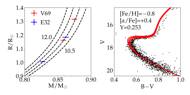
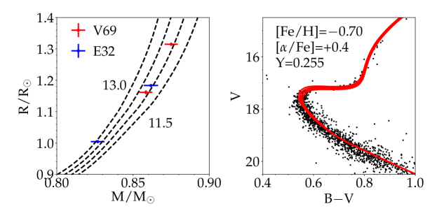
Figure 7: Comparison in the mass-radius plane (left) and the CMD (right) of Dartmouth isochrones for a range of ages. The upper and lower limits in age are given on the mass-radius plots and the difference in age between successive isochrones is 0.5 Gyr. The same isochrones are shown again in the B$-$V CMD on the right, plotted over the photometry from TK10. For the CMD analysis we use the adopted true distance modulus (13.224) and adopted reddening value E(B$-$V)=0.03 as in Section 6.1. [Fe/H] increases from top to bottom at fixed [$\alpha$/Fe]. The isochrones that bracket the DEBs on the left are compared to the CMD on the right. Error bars of the radii are only slightly larger than the dots marking component locations in the $M-R$ plane.

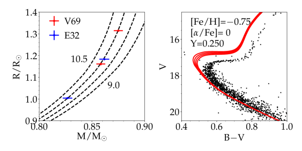
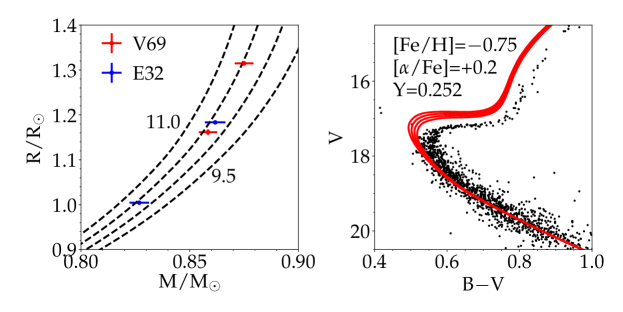
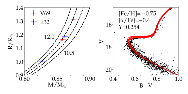
Figure 8: Similar to Figure 7 except that now [$\alpha$/Fe] varies at fixed [Fe/H].

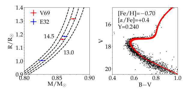
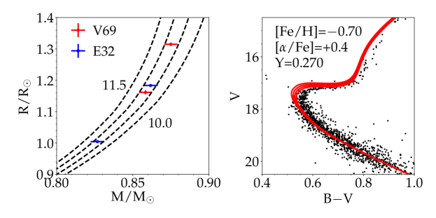
Figure 9: Similar to Figures 7 and 8 except that now Y varies at fixed [Fe/H] and [$\alpha$/Fe].

Appendix A Details of period determination

Our timing analysis proceeded in four steps.

Step 1: We plotted the light curves separately for each filter and eclipse. Inspecting by eye and taking into account different widths and depths of eclipses we estimated approximate times of minima and their primary/secondary type. This yielded 12 times of minima. The spectroscopic period derived in Section 2.1 proved sufficiently accurate to derive a unique cycle count. A least squares fit yielded an approximate ephemeris $T_{min}=T_{0}+P\times E+II_{min}\times\Delta t$:

$$\begin{split}T_{min}&=2457246.221(11)+40.9124(6)\times E\\ &+II_{min}\times 20.316(19).\end{split}$$ (4)

where $II_{min}=0$ or 1 for primary and secondary eclipses, respectively. This demonstrated the consistency of spectroscopic and photometric periods, and, as the minima were not equidistant in phase, confirmed the nonzero eccentricity of the orbit.

Step 2: To improve the ephemeris (4) we transformed all observations to a common rectified light curve and attempted fitting it with a unique analytical curve.
2a: From magnitudes in each filter $F$ we subtracted the average magnitude at maximum light in that filter, and multiplied the result by the ratio $c_{F}$ of the eclipse depth in $F$ to that in $V$, so that the rectified magnitudes were

$$m_{rect}(t)=[m_{F}(t)-m_{F,max}]c_{F},$$ (5)

where $F=V,B,I$ and $c_{V}=1$ by construction. Initially we adopted $c_{B}=c_{I}=1$.
2b: A brute force Fourier series approach would suffer from loss off degrees of freedom due to excessive number $n_{h}$ of harmonics needed to fit eclipses and prevent the Gibbs effect. To mitigate the range of harmonics we compressed the rectified light curve by transforming the orbital phase $\varphi=(t-T_{0})\omega$, where $\omega=2\pi/P$ is the orbital angular frequency, to a new scale $\phi$ defined by

$$\phi=\frac{1}{2}[\tau(\varphi)+\tau(\varphi-\Delta\varphi)],$$ (6)

where $\Delta\varphi=\omega\Delta t$ is the phase difference between eclipses, and

$$\tau(\varphi)=\Gamma\int_{0}^{\frac{\varphi}{2}}(\cos x)^{2l}dx.$$ (7)

Note that $\phi$ varies slowly at the maximum light of the system, and relatively quickly during the minima. The constant $\Gamma$ was chosen so that

$$\tau(\varphi+2\pi)=\tau(\varphi)+2\pi.$$ (8)

The integral in (7) was evaluated by means of Gradshteyn & Ryzhik (1971) formula 2.512.2. Subsequent experiments demonstrated that $l=90$ was a good choice. This corresponds to a severe compression of the light curve beyond a time interval $\delta t$ from minima, where for $x=\omega\delta t$ the inequality $-1>\ln(\cos^{2l}x)\approx-lx^{2}$ yields

$$\delta t>\frac{1}{\omega\sqrt{l}}\approx 0.7d$$ (9)

2c: To finish Step 2 we fitted the compressed rectified light curve $m_{rect}(\phi)$ with a series of Szegö orthogonal polynomials Schwarzenberg-Czerny (1996, 2012). A series of 25 polynomials, equivalent to $n_{h}=12$ harmonics, sufficed to fit the light curve while accounting for the different widths of the two eclipses.

Step 3: Residuals from the polynomial fit in step 2c may be minimized by adjusting $\omega$, $c_{B}$ and $c_{I}$ by nonlinear least squares fitting. For this purpose, numerical derivatives of the residuals were calculated by repeating Step 2 with perturbed $\omega$, $c_{B}$ and $c_{I}$. Although this sufficed for the present purpose, we note that analytical recurrence formulae may be obtained for the derivatives of Szegö polynomials and $\tau(\phi)$.

Step 4: To continue, we needed to obtain improved values of $T_{0}$ and $\Delta\varphi$ for use at 2a. Using new values of $\omega$, $c_{B}$ and $c_{I}$ to recalculate $m_{rect}$, and returning to the ordinary phase scale $\varphi$, we applied the method of Kaluzny et al. (2015) to find central phases of both eclipses separately. The method is essentially that of Kwee & van Woerden (1956), improved by an interpolation of light curve with Szegö polynomials in ordinary phases $\varphi$.

Several iterations of Steps 2, 3 and 4 led to convergence, yielding $c_{B}=0.991(6)$, $c_{I}=1.008(4)$, and the final ephemeris given by Equation (1). The derived values of $c_{B}$ and $c_{I}$ are close to 1, which confirms the closing remark of Section 2.2 that the temperatures of the components must be nearly equal.

Appendix B Further arguments for the membership of E32 in 47 Tuc

With the $Gaia$ PM of 47 Tuc equal to ($5.2477\pm 0.0016$, $-2.5189\pm 0.0015$) mas/y (Helmi et al., 2018) the cluster-centric proper motion (CCPM) of E32 is ($0.28\pm 0.21$, $0.88\pm 0.19$) mas/y, i.e. $0.92\pm 0.21$ mas/y in total. However, this value should be treated with some caution, as the final accuracy of Gaia PM measurements in globular clusters is expected to be reached only in a few years time (Pancino et al., 2017). The ground-based data of Narloch et al. (2017) and HST data of Heyl et al. (2017) yielded upper CCPM limits of, respectively, 0.44 mas/y and 0.08 mas/y (Heyl, private communication). A weighted mean from the three measurements is $0.33\pm 0.07$ mas/y, which at a parallax of 0.225 mas translates into $7.0\pm 1.6$ km s^-1. The corresponding 3D-velocity of E32 with respect to 47 Tuc is $22.7\pm 1.7$ km s^-1, and is equal to the escape velocity from $R_{e}=9.7$′ (Heyl et al., 2017).

Neglecting small departures of 47 Tuc from spherical symmetry one can estimate the probability that the binary resides beyond $r_{e}$, i.e. is unbound, by

$$P_{\mathrm{u}}=\frac{\int_{A}^{B}n(r(x))dx}{\Sigma(R_{0})}<\frac{\int_{C}^{D}n(r(x))dx}{\Sigma(R_{0})}=\frac{\Sigma(R_{e})}{\Sigma(R_{0})}\approx 0.03,$$ (10)

where $n$ is the number density of cluster stars, $\Sigma$ is the column density of cluster stars, the inequality holds for the same reason for which spherically symmetric planetary nebulae are observed as rings rather than spheres, and the values of $\Sigma$ are taken from Lane, Küpper & Heggie (2012). If we calculate the 3D velocity using the $Gaia$ PM value, the escape radius shrinks to 5′.2, causing the upper limit of $P_{\mathrm{u}}$ to increase to $\sim$0.7. However, we think that in such a case the first three arguments taken together would be strong enough to suggest that E32 is a recent escaper from the cluster. It is also worth mentioning that two stars moving even faster than E32 were discovered in 47 Tuc by Meylan, Dubath & Mayor (1991), who found them to be likely cluster members which were recently accelerated. The case of high-velocity stars in globular clusters was discussed in detail by Lützgendorf et al. (2012), who concluded that the most likely accelaration mechanism is a close encounter with a $\sim$10 $M_{\odot}$ black hole.

Figure 10: Schematic view of a plane defined by E32 (star) and the line of sight between the observer and the center of 47 Tuc. See Section 5 for discussion.

Appendix C Sky charts

References

- Brogaard et al. (2012) Brogaard, K., VandenBerg, D.A., Bruntt, H., Grundahl, F., et al. 2012, A&A, 543, 106 (B12)
- Brogaard et al. (2017) Brogaard, K., VandenBerg, D.A., Bedin, L.R., Milone, A.P., Thygessen, A., Grundahl, F., 2017, MNRAS, 468, 645 (B17)
- Bernstein et al. (2004) Bernstein R., Shectman S.A., Gunnels S.M., Mochnacki S., Athey A.E., 2003, Proc. SPIE, 4841, 1694
- Brown et al. (2018) Brown A.G.A. et al., 2018, A&A, 616, A1
- Casagrande et al. (2010) Casagrande L., Ramírez I., Meléndez J., Bessell M., Asplund M., 2010, A&A, 512, A54 (C10)
- Casagrande & VandenBerg (2014) Casagrande L., VandenBerg, D.A., 2014, MNRAS, 444, 392
- Chen et al. (2018) Chen S., Richer H., Caiazzo I., Heyl J., 2018, ApJ, 867, 132
- Claret (2000) Claret A., 2000, A&A, 363, 1081
- Coelho et al. (2005) Coelho P., Barbuy B., J. Meléndez J., Schiavon R. P., Castilho B. V., 2005, A&A, 443, 735
- Dotter et al. (2008) Dotter A., Chaboyer B., Jevremović D., Kostov V., Baron E., Ferguson J.W. 2008, ApJS, 178, 89
- Dotter et al. (2009) Dotter A., Kaluzny, J., & Thompson, I., 2009, IAUS, 258, 171 (D9)
- Graczyk et al. (2017) Graczyk D., Konorski P., Pietrzyński G., Gieren W., Storm J. et al., 2017, ApJ, 837, 7
- Graczyk et al. (2019) Graczyk D., Pietrzyński G., Gieren W., Storm J., Nardetto N. et al., 2019, ApJ, 872, 85
- Gradshteyn & Ryzhik (1971) Gradshteyn I.S., Ryzhik I.M., 1971, Table of Integrals, Series and Products. Nauka Publishers, Moscow
- Harris (1996) Harris W.E., 1996, AJ, 112, 1487 (H96)
- Helmi et al. (2018) Helmi et al. 2018, A&A, 616, 12
- Heyl et al. (2017) Heyl J., Caiazzo I., Richer H., Anderson J., Kalirai J., Parada J., 2017, ApJ, 850, 186
- Kaluzny et al. (2006) Kaluzny J., Pych W., Rucinski S., Thompson I.B., 2006, Acta Astron, 56, 237
- Kaluzny et al. (2013a) Kaluzny J., Rozyczka M., Pych W., Krzeminski W., Zloczewski K. et al., 2013a, Acta Astron., 63, 309
- Kaluzny et al. (2013b) Kaluzny J. Thompson I.B., Rozyczka M., Dotter A., Krzeminski W. et al., 2013b, AJ, 145, 43
- Kaluzny et al. (2002) Kaluzny J., Thompson I.B. Krzeminski W., Olech A., Pych W., Mochejska, B., 2002, ASP Conf. Ser. 265, Omega Centauri, A Unique Window into Astrophysics, ed. F. can Leewen, J. D. Hughes, G. Piotto (San Francisco, CA: ASP), 155
- Kaluzny et al. (2014) Kaluzny J., Thompson I.B., Dotter A., Rozyczka M., Pych W. et al., 2014, Acta Astron., 64, 11
- Kaluzny et al. (2015) Kaluzny J., Thompson I.B., Dotter A., Rozyczka M., Schwarzenberg-Czerny A., 2015, AJ, 150, 155
- Kwee & van Woerden (1956) Kwee K.K., van Woerden H., 1956, BAN, 12, 327
- Lane, Küpper & Heggie (2012) Lane R.R., Küpper A.H.W., Heggie D.C., 2012, MNRAS, 423, 2845
- Lützgendorf et al. (2012) Lützgendorf N., Gualandris A., Kissler-Patig M., Gebhardt K., Baumgardt H. et al., 2012, A&A, 543, A82
- Meylan, Dubath & Mayor (1991) Meylan G., Dubath P., Mayor, M., 1991, ApJ, 383, 587
- Narloch et al. (2017) Narloch W., Kaluzny J., Poleski R., Rozyczka M., Pych W., Thompson I.B., 2017, MNRAS, 471, 1446
- Paczyński (1997) Paczyński B., 1997, in Space Telescope Science Institute Series, The Extragalactic Distance Scale, ed. M. Livio (Cambridge: Cambridge Univ. Press), 273
- Pancino et al. (2017) Pancino E., Bellazzini M., Giuffrida G., Marinoni S., 2017, MNRAS, 467, 412
- Pietrzyński et al. (2019) Pietrzyński G., Graczyk D., Gallenne A., Gieren W., Thompson I. B. et al., 2019, Nature, 567, 200
- Persson et al. (2013) Persson, S. E. et al., 2013, PASP, 125, 654
- Rozyczka et al. (2014) Rozyczka M., Kaluzny J., Thompson I.B., Dotter A., Pych W., Narloch W., 2014, Acta Astron., 64, 233
- Rucinski (2002) Rucinski S.M., 2002, AJ, 124, 1746
- Schlafly & Finkbeiner (2011) Schlafly, E.F., Finkbeiner, D.P., 2011, ApJ, 737, 103
- Schwarzenberg-Czerny (1996) Schwarzenberg-Czerny, A., 1996, ApJ, 460, L107
- Schwarzenberg-Czerny (2012) Schwarzenberg-Czerny, A., 2012, New Horizons in Time-Domain Astronomy, IAU Symposium 285, 81
- Shao & Li (2019) Shao, Z. & Li, L., 2019, MNRAS, 489, 3093
- Skrutskie et al. (2006) Skrutskie, M.F, Cutri, R.M, Stiening, R., Weinberg, M.D., Schneider, S. et al., 2006, AJ,131, 116
- Southworth (2013) Southworth J., 2013, A&A, 557, A119
- Stetson (1987) Stetson, P.B., 1987, PASP, 99, 191
- Stetson (1990) Stetson, P.B., 1990, PASP, 102, 932
- Thompson et al. (2001) Thompson I.B., Kaluzny J., Pych W., Burley G.S., Krzeminski W. et al., 2001, AJ, 121, 3089
- Thompson et al. (2010) Thompson I.B., Kaluzny J., Rucinski S.M., Krzeminski W., Pych W., Dotter A., Burley G.S., 2010, AJ, 139, 329 (TK10)
- Udalski, Szymański & Szymański (2015) Udalski A., Szymański M.K., Szymański G., 2015, Acta Astron., 65, 1
- VandenBerg & Clem (2003) VandenBerg, D.A., Clem, J.L., 2003, AJ, 126, 778
- Zucker & Mazeh (1994) Zucker, S., Mazeh, T., 1994, ApJ, 420, 806