Noisy voter model for the anomalous diffusion of parliamentary presence

Abstract

We examine parliamentary presence data of the 2008–2012 and the 2012–2016 legislatures of Lithuanian parliament. We consider cumulative presence series of each individual representative in the data set. These series exhibit superdiffusive behavior. We propose a modified noisy voter model as a model for the parliamentary presence. We provide detailed analysis of anomalous diffusion of the individual agent trajectories and show that the modified model is able to reproduce empirical statistical properties.

1 Introduction

Numerous processes observed in variety of physical systems have been known to diffusive faster or slower than the classical Brownian particle. This family of process is often referred to as anomalous diffusion. In one dimensional case the anomalous diffusion would be characterized by the root mean square displacement (standard deviation) of the following dependence on time:

$$\sqrt{\left\langle\left(\Delta x\right)^{2}\right\rangle}\sim t^{\alpha},$$ (1)

where $\Delta x$ is the distance the diffusing particle has moved away from the origin with the average being taken over ensemble of particles. For the classical Brownian motion (normal diffusion) we would have $\alpha=\frac{1}{2}$. A process with slower diffusion, $\alpha<\frac{1}{2}$, would be considered to be subdiffusive. Subdiffusion is often assumed to be caused by the particles jumping from one local minima, being trapped for a prolonged period of time and then jumping to another local minima [1, 2, 3, 4]. Processes exhibit superdiffusion if the diffusion is faster than the normal diffusion, with $\alpha>\frac{1}{2}$. Superdiffusion is often assumed to be observed in diffusive processes exhibiting Levy flights [1, 5, 6, 7]. Another possible causes behind anomalous diffusion could be time subordination [8, 9, 10, 11] and heterogeneity in the media [12, 13, 14]. Here we will consider anomalous diffusion in the parliamentary presence data. Similar analysis was already conducted by [15] using Brazilian parliamentary presence data. Reportedly, strong evidence for the ballistic regime, $\alpha\approx 1$, was found. In regards to anomalous diffusion our approach to analysis is mostly similar, but we use Lithuanian parliamentary presence data. Furthermore we also consider other statistical properties of the empirical data, such as attendance streak distributions, which provide additional information about the process as well as additional way to validate a model.

In [15] a phenomenological model for the parliamentary presence was proposed by the means of a non–linear diffusion equation. Here we propose an agent–based model for the parliamentary presence. At its core the proposed agent–based model is the voter model. The voter model and variety of its modifications have been under active consideration by opinion dynamics (sociophysics) community [16, 17, 18]. Such as the impact of inflexibility [19, 20], spontaneous flipping [21, 22], variety of network topology effects [23, 24, 25, 26, 27, 28], private opinions [29, 30, 31], nonlinear interactions [32, 33] were studied in the framework of the voter model. Various voter models were applied to model electoral and census data [34, 35, 36, 37, 38] as well as to model financial markets [39, 40, 41, 42, 43, 44, 45]. Anomalous diffusion, to the best of our knowledge, was not studied in any of the voter models, because these models should not exhibit anomalous diffusion. Yet our approach takes a different point of view than is common in the analysis of the voter models, here we consider individual agent trajectories. From this point of view observing anomalous diffusion is quite possible.

Our goal in this paper is to understand anomalous diffusion in the parliamentary presence data in the context of the voter models. Having this goal in mind we have organized the paper as follows. In Section 2 we conduct empirical analysis, which helps us to provide context for the numerical modeling of the parliamentary presence phenomenon. In Section 3 we describe the noisy voter model and its modifications. In Section 4 we analyze anomalous diffusion of the individual agents trajectories and show that the model is able to reproduce the empirical observations. We provide concluding remarks and discussion in Section 5.

2 Empirical analysis of the parliamentary presence data

We have obtained the registration to vote data, which indicates willingness of the representative to vote on the agenda, from the Lithuanian parliament’s website [46]. Based on the data we have constructed presence time series, $\eta_{t}^{\left(i\right)}$, for each of the representatives in the Lithuanian parliament (index $i$ loops through the representatives, while index $t$ is the session number). We assume that representative was absent during the session, if the representative did not register to vote at all during that session, and encode this as $0$. Otherwise we assume that representative was present and encode this as $1$.

The raw registration to vote data also indicates whether the representative was elected (the seat taken) at the time of the session. Reasons why a particular seat could be empty vary: death, prosecution or being elected to a different post. While the replacements are elected as soon as possible, we still have to deal with some missing data. Unlike in [15], we detect the replacements and join the respective presence time series. Suppose that representative A left his seat after $t_{A}$ sessions, his possible replacements would be all representatives who have taken their seats after $t_{A}$ sessions. Among all representatives who were not present till the end of their term, we find those with the least possible replacements (though the number of possible replacements should be larger $1$). If there are multiple possible replacements, we select the one who took their seat the earliest and join the records of both representatives. We proceed until all replacements are found (at this point the data set contains $141$ records). This procedure should minimize the number of records with the missing data, yet if at this point some data is still missing, then we replace the records containing missing data with the copies of valid records. Average replacement percentage for both considered legislatures was around $10\%$. The reported results are robust in respect to this random replacement procedure. Due to the replacement scheme our data sets always have exactly $141$ presence time series (as there $141$ seats in the Lithuanian parliament). We have made the processed attendance data set for the legislatures of 2008–2012 and 2012–2016 available via GitHub repository [47].

As in [15] we take primary interest in the cumulative presence series, which are obtained directly from $\eta_{t}^{\left(i\right)}$ series and are defined as:

$$x_{t}^{\left(i\right)}=x_{t-1}^{\left(i\right)}+\eta_{t}^{\left(i\right)}.$$ (2)

Note that in the begging of each legislature we reset the attendance record, $x_{0}^{\left(i\right)}=0$, for each representative. Using the cumulative series we observe the temporal evolution of its mean (over individual representatives at a particular time):

$$\mu_{t}=\frac{1}{N}\sum_{i=1}^{N}x_{t}^{\left(i\right)},$$ (3)

and its standard deviation (over individual representatives at a particular time):

$$\sigma_{t}=\sqrt{\frac{1}{N-1}\sum_{i=1}^{N}\left[x_{t}^{\left(i\right)}-\mu_{t}\right]^{2}}.$$ (4)

See Fig. 1 for example of the empirical $x_{t}^{\left(i\right)}$ series and the empirical $\mu_{t}$ and $\sigma_{t}$ series. As one should expect, due to the way we have encoded $\eta_{t}^{\left(i\right)}$ as well as due to high average presence rates ($\sim 90\%$ in both cases), the mean grows linearly with time $\mu_{t}\sim t$. While the standard deviation clearly shows the superdiffusive behavior, $\sigma_{t}\sim t^{\alpha}$ with $\alpha=0.85$. Note that the previous analysis of the Brazilian parliament presence data [15] reported that the ballistic regime, $\alpha\approx 1$, was found for the standard deviation. This difference could be related to the different treatment of the missing data as well as to the differences between Lithuanian and Brazilian parliaments. There are other possible reasons related to the individual level dynamics, which are discussed in the following sections.

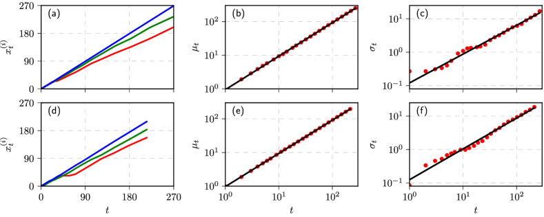
Figure 1: Exemplary presence time series ((a) and (d)), mean ((b) and (e)) and standard deviation ((c) and (f)) series for the 2008–2012 legislature ((a), (b) and (c)) and 2012–2016 legislature ((d), (e) and (f)) data. Red dots ((b), (c), (e) and (f)) represent empirical data, while black lines provide power–law fits with exponents $\alpha=1$ ((b) and (e)) and $\alpha=0.85$ ((c) and (f)).

Closer examination of Fig. 1 (c) reveals that some correlation in the residuals is present. This is likely related to the limited amount of empirical data: both in temporal sense (our data sets cover slightly more than $200$ parliamentary sessions) and realization sense (our data sets include $141$ attendance records).

We supplement our empirical analysis by considering presence, $T_{p}$, and absence, $T_{a}$, streaks of the individual representatives (see Fig. 2). Shorter streaks, $T_{p}<100$ and $T_{a}<10$, seem to be distributed exponentially, suggesting that underlying process could be a Poisson process. While the longer streaks break the trend indicating that underlying process might be a non–homogeneous Poisson process or a non–Poisson process. In the next section we introduce an agent–based model driven by a Poisson process, which is non–homogeneous in time.

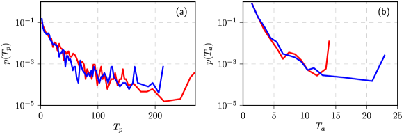
Figure 2: Probability density functions of the length of presence, $T_{p}$, (a) and absence, $T_{a}$, (b) streaks in the presence data set for the 2008–2012 (red curves) and 2012–2016 (blue curves) legislatures.

3 Noisy voter model of the parliamentary presence

Original definition of a model, which is now known as the voter model, involved only a simple replacement mechanism [48]. The replacement mechanism was assumed to represent competition between two species, but it can also represent competition between social ideas or behaviors. In fact the model has found wider recognition in opinion dynamics community and therefore is known as the voter model [49, 16]. While it is quite easy to imagine direct competition between two species, competition between the ideas is indirect instead. It happens only because social animals, e.g., humans, tend to exert social pressure on each other, which is the force to causing the replacement of less popular ideas by the more popular ones. Though, admittedly there are a few possible ways to respond to social pressure [50, 21, 51], which can have profound effects on the observed dynamics. We believe that the voter model with noise is the simplest model, which directly includes both social conformity and independence mechanisms and indirectly takes into account anti–conformist behavior. In our earlier works we have shown that the noisy voter model is quite applicable both to finance [41, 42, 44] and opinion dynamics [36, 38]. Here we apply the noisy voter model to model the parliamentary presence.

Let us assume that after each session each member of the parliament reconsiders his previous behavior. If the representative had intended to attend (let us label this state as $1$), then the representative could begin to intend to skip (let us label this state as $0$). Let this transition occur with probability:

$$p_{1\rightarrow 0}^{\left(i\right)}=h\left[\varepsilon_{0}+\frac{X_{0}}{N}\right].$$ (5)

Likewise, if the representative intended to skip, then the representative could start to intend to attend. Let this transition occur with probability:

$$p_{0\rightarrow 1}^{\left(i\right)}=h\left[\varepsilon_{1}+\frac{X_{1}}{N}\right]=h\left[\varepsilon_{1}+\left(1-\frac{X_{0}}{N}\right)\right].$$ (6)

In both of the transition probabilities above $h\cdot\varepsilon_{k}$ are the independent switching probabilities to the state labeled by $k$, while $h\cdot\frac{X_{k}}{N}$ are the imitation switching probabilities to the state labeled by $k$ (these transitions happen due to influence of peers in the destination state). Effectively $h$ sets the rate at which the agents change their state (the higher $h$ is the faster the changes become), while $\varepsilon_{k}$ controls the impact of peer pressure on the changes (the larger $\varepsilon_{k}$ the more independent of peer pressure changes become). Due to conservation of total number of agents, $N$, we have $X_{1}=N-X_{0}$ (here $X_{k}$ is the total number of agents in the state $k$). We consider only those parameter values for which neither of the transition probabilities for any $X_{0}\in\left[0,N\right]$ is larger than one.

Then just before the session each agent decides how to act (whether to actually attend). Let the agent attend with probability $q_{k}$ given he is in the state $k$. In general $q_{k}$ can take any values between $0$ and $1$, we only requite that $q_{1}\geq q_{0}$ as agents in state $1$ are assumed to have an intent to attend.

This model can be seen as a special case of hidden Markov model [52]. Yet in our case each individual agent is described by its own hidden Markov model: internal (intent) and observed (action) states describe individual agents and not the whole system. In Fig. 3 we have shown a representation of the model dynamics from an individual agent perspective as hidden Markov model. It is important to note that $p_{i\rightarrow j}$ depend on the intent of other agents, while $q_{i}$ probabilities remain constant through out the simulation.

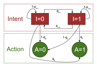
Figure 3: Representation of the model dynamics from an individual agent perspective. Here $I$ represents the internal intent state and $A$ represents the observed action state.

In this formulation of the noisy voter model more than one agent can change its state after each time tick (which corresponds to a parliamentary session in our case). This contrasts with the original formulation of the voter model, which allows for just one agent to change state during a single time tick. Original one–step formulation could be seen as superior in a sense that it allows for the continuous time treatment by the Gillespie method [53, 54]. A similar formulation to the one used here was proposed in [55] and compared against the Bass diffusion model, which is known to be unidirectional (with one agent state being absorbing) variant of the noisy voter model [56]. It was found that the models produce very similar time series, but allowing for multiple agents to switch per step introduces information lag into the model.

The model we have introduced here also bears certain similarities to the voter models with private and public opinions [29, 30, 31]. Our approach is different, because we have the true state (or intent), which is driven by the imitation behavior as it would be in any voter model, and the observed state (or action), which is randomly taken by the agent with probability depending on the true state. Another similarity can be drawn to [57] in which agents have continuous opinions, but act using discrete actions. In our approach agents have discrete opinions as agent states are binary.

We have shared an implementation of the model in Python via GitHub repository [58].

4 Anomalous diffusion of individual agent trajectories in the noisy voter model

Let us discuss the anomalous diffusion between individual agent trajectories this model exhibits when applied as a model for parliamentary presence. First of all for a variety of valid parameter sets we have observed a linear trend in the mean series, $\mu_{t}$. While the trends of the standard deviation series, $\sigma_{t}$, are a bit more sophisticated.

Let us start by considering the simplest case of the proposed model. Namely, let us assume that the intent of agents is pure, i.e., they either always skip, $q_{0}=0$, or attend, $q_{1}=1$, if they intend to do so. Furthermore let us assume that the true states are equally attractive for agents switching independently, i.e., let $\varepsilon_{0}=\varepsilon_{1}=\varepsilon$. In this highly simplified case we observe that $\sigma_{t}$ exhibits the following scaling behavior:

$$\sigma_{t} =\frac{\theta_{0}t}{\sqrt{\theta_{1}+St}}.$$ (7)

In the above $\theta_{0}$ and $\theta_{1}$ seem to be independent of the model parameters (we estimate that $\theta_{0}=0.66\pm 0.06$ and $\theta_{1}=1.4\pm 0.55$), while $S$ seems to be fully determined by the model parameters (the form was determined numerically),

$$S=h\left(1+2\varepsilon\right).$$ (8)

Note that $S$ equals the sum of the transition probabilities. It should be quite easy to see that on the shorter time scales the model exhibits ballistic regime, $\sigma_{t}\sim t$, while on the longer time scales normal diffusion, $\sigma_{t}\sim\sqrt{t}$, takes over. In Fig. 4 we have shown that this scaling law rather nicely fits numerical results obtained with different values of the model parameters. In Fig. 4 (b) the difference between the numerical results representing two smallest $\varepsilon$ is quite small. This is expected as $S$ changes very little with $\varepsilon$ in those cases, because large $N$ dominates the change in $\varepsilon$.

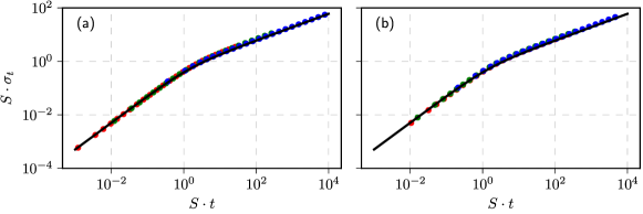
Figure 4: Scaling behavior of $\sigma_{t}$ in the simplest case (with $\varepsilon_{0}=\varepsilon_{1}=\varepsilon$, $q_{0}=0$ and $q_{1}=1$) of the model: numerical results (colored dots) and the scaling law, Eq. (7), (black curves). Scaling law parameter values: $\theta_{0}=0.66$ and $\theta_{1}=1.4$. Default model parameter values: $\varepsilon=0.1$, $h=10^{-2}$, $N=141$. Subfigure (a) shows the scaling behavior in respect to $h$ with the following values: $10^{-3}$ (red dots), $10^{-2}$ (green dots) and $3\cdot 10^{-1}$ (blue dots). Subfigure (b): $\varepsilon=0.03$ (red dots), $3$ (green dots) and $10$ (blue dots).

Breaking the symmetry assumption, i.e., allowing for $\varepsilon_{0}\neq\varepsilon_{1}$, does not break the qualitative behavior of the scaling law. Though, we need to rewrite the scaling multiplier as

$$S=h\left(1+\varepsilon_{0}+\varepsilon_{1}\right),$$ (9)

and also $\theta_{0}$ value changes as the scaling law shifts downwards (see Fig. 5). This downward shift is expected as in the asymmetric case agents tend to prefer one state over the other (majority of them gather in the same state), thus decreasing $\sigma_{t}$ on all time scales. To highlight this shift in Fig. 5 we have shown both scaling law used for the symmetric case (dashed curve) and for the extremely asymmetric case (solid curve).

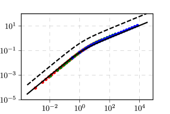
Figure 5: Scaling behavior of $\sigma_{t}$ in the asymmetric simplified case (with $q_{0}=0$ and $q_{1}=1$) of the model: numerical results (colored dots) and the scaling law, Eq. (7), (black curves). Scaling law parameter values: $\theta_{0}=0.66$ (dashed curve) and $0.12$ (solid curve), $\theta_{1}=1.4$ (dashed curve and solid curve). Model parameter values: $\varepsilon_{0}=0.1$, $\varepsilon_{1}=10$ and $N=141$ (all cases), $h=10^{-4}$ (red dots), $10^{-3}$ (green dots) and $3\cdot 10^{-2}$ (blue dots).

Finally let us also relax the pure intent assumption by assuming that there is probability $q$ with which agent’s intent is pure, i.e., let $q_{1}=q$ and $q_{0}=1-q$. Still this impure intent assumption provides us a simplified version of the model as the impure intent probability $q$ is assumed to be homogeneous. In general case, which we will later use to fit the empirical data, $q_{0}$ and $q_{1}$ can take any value between $0$ and $1$ (as long as $q_{1}\geq q_{0}$). The impure intent assumption is the final ingredient of the model, which enables us to change the nature of diffusion in the short time scale region. Though it is worth to note that, this is also the only model mechanism which acts in discrete time. All other model mechanisms would work the same way even if we would redefine the model in continuous time, but it would impossible to redefine this mechanism for the continuous time case without making any additional assumptions. Hence the impact of $q$ is not trivial. For large values of $S$ it has no impact, because the model is in the normal diffusion regime even with $q=1$. For really small $S$ having $q<1$ introduces normal diffusion on the shortest time scales, then on the intermediate time scales ballistic regime is observed and finally on the longest time scales once again normal diffusion takes over (see Fig. 6 (a)). For intermediate $S$ having $q<1$ allows for superdiffusive behavior (see Fig. 6 (b)), which we have observed in the empirical data.

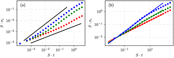
Figure 6: Scaling behavior of $\sigma_{t}$ in the model with impure intent ($q_{0}=1-q$ and $q_{1}=q$) in respect to $q$: numerical results (colored dots) and power law fits (lines). Model parameter values: $q=0.5$ (red dots), $0.57$ (green dots) and $0.68$ (blue dots), $\varepsilon_{0}=\varepsilon_{1}=0.06$, $N=141$ (all in both cases), $h=1.5\cdot 10^{-4}$ (a) and $1.5\cdot 10^{-2}$ (b). Power law fits (a) have the following exponents: $\alpha=0.5$ (bottom curve) and $1$ (upper curve). Power law fits (b): $\alpha=0.5$ (red curve), $0.6$ (green curve) and $0.75$ (blue curve).

This analysis provides some qualitative insights into the various behaviors one could observe in the empirical presence data. Yet our goal in this paper is to match not only $\sigma_{t}$ series, but also presence quantile series (as a proxy for the temporal evolution of the presence distribution) and attendance streak distributions. Therefore we have performed random parameter space sweep, which was somewhat informed by the previous analysis, and were able to find model parameter set, which generates presence records with statistical properties similar to those observed in the empirical data (see Figs. 7, 8 and 9). Presence quantiles, as expected, exhibit linear growth trends and the overlap between the empirical data and the numerical results is rather good (see Fig. 7). We were also able to quite precisely reproduce the superdiffusive behavior of the records as well (see Fig. 8). Presence streak distribution is also reproduced rather nicely (see Fig. 9 (a)). The only evident disagreement between the model and the empirical data is the absence streak distribution, which was observed to be noticeably broader in the empirical data. This discrepancy might be attributed to the small size of the empirical data, but also to a more complicated dynamics of being absent. Namely, the proposed model does not take into account specific circumstances, which are not directly related to the social aspects of attendance. Such circumstances may include sickness leaves, business or leisure trips, which in these cases the representative would skip multiple sessions during that period.

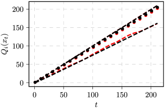
Figure 7: Presence quantile, $0.025$ (dashed curves), $0.5$ (points) and $0.975$ (dashed curves), series observed in the empirical data (red) and the model (black). Empirical data averaged over both considered legislatures. Model parameter values: $h=7.1\cdot 10^{-4}$, $\varepsilon_{0}=0.21$, $\varepsilon_{1}=0.43$, $q_{0}=0.8$, $q_{1}=0.98$.

Figure 8: Standard deviation series $\sigma_{t}$ in the empirical data (red dots) and the model (black curve). Empirical data averaged over both considered legislatures. Model parameters are the same as in Fig. 7.

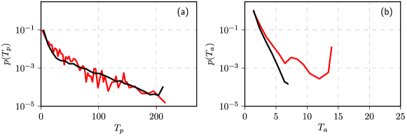
Figure 9: Probability density functions of the length of presence, $T_{p}$, (a) and absence, $T_{a}$, (b) streaks in the empirical data (red curves) and the model (black curves). Empirical data averaged over both considered legislatures. Model parameters are the same as in Fig. 7.

5 Conclusions

We have analyzed the parliamentary presence data for the Lithuanian parliament legislatures of 2008–2012 and 2012–2016. A similar analysis was conducted earlier [15] using Brazilian parliamentary presence data. Unlike [15] we haven’t found linear trend in standard deviation series (so–called ballistic regime), but instead we have found sub–linear trend. Though the trend is faster than would be expected from the normal diffusion, therefore we can conclude that the considered empirical data exhibits superdiffusive behavior. To complement the empirical analysis we have also examined the distribution of the presence and absence streaks in the data. We have found that both streak distributions are reasonably close to an exponential distribution for the shortest time scales, but we have also observed fatter tails.

To replicate selected statistical properties of the empirical data we have built a simple agent–based model, which is built upon the voter model. Unlike most models built upon the voter model, this model involves two state dynamics, where one state is the true state (intent) of the agent while the other is the observed state (action) of the agent. While such voter models are not novel, the application and the point of view taken here are. Voter models were not considered from the anomalous diffusion point of view, because the whole system trajectories evidently would not exhibit anomalous diffusion, but here we have shown that distinct agent trajectories can. In our analysis whenever we have considered only the true state dynamics, we have observed only ballistic regime or normal diffusion. Adding the second, noisy observation, state to the model have helped us to introduce superdiffusion of the distinct agent trajectories. The proposed model not only successfully reproduced the observed superdiffusive behavior, but was also able to reproduce presence quantile series and attendance streak distributions. The proposed model could also reproduce the ballistic regime as observed in the Brazilian data set, though values of $q_{0}$ and $h$ would likely be smaller (implying more truthfulness as well as slower changing of the intent).

References

- [1] R. Metzler, J. Klafter, The random walk’s guide to anomalous diffusion: a fractional dynamics approach, Physics Reports 339 (1) (2000) 1 – 77. doi:10.1016/S0370-1573(00)00070-3.
- [2] O. Chepizhko, F. Peruani, Diffusion, subdiffusion, and trapping of active particles in heterogeneous media, Physical Review Letters 111 (2013) 160604. doi:10.1103/PhysRevLett.111.160604.
- [3] F. Evers, C. Zunke, R. D. L. Hanes, J. Bewerunge, I. Ladadwa, A. Heuer, S. U. Egelhaaf, Particle dynamics in two-dimensional random-energy landscapes: Experiments and simulations, Physical Review E 88 (2013) 022125. doi:10.1103/PhysRevE.88.022125.
- [4] J. Iaconis, S. Vijay, R. Nandkishore, Anomalous subdiffusion from subsystem symmetries, Physical Review B 100 (2019) 214301. doi:10.1103/PhysRevB.100.214301.
- [5] N. Mercardier, W. Guerin, M. Chevrollier, R. Kaiser, Lévy flights of photons in hot atomic vapours, Nature Physics 5 (2009) 602–605. doi:10.1038/nphys1286.
- [6] C. Scalliet, A. Gnoli, A. Puglisi, A. Vulpiani, Cages and anomalous diffusion in vibrated dense granular media, Physics Review Letters 114 (2015) 198001. doi:10.1103/PhysRevLett.114.198001.
- [7] E. I. Kiselev, J. Schmalian, Lévy flights and hydrodynamic superdiffusion on the Dirac cone of graphene, Physical Review Letters 123 (2019) 195302. doi:10.1103/PhysRevLett.123.195302.
- [8] H. C. Fogedby, Langevin equations for continuous time Lévy flights, Physical Review E 50 (1994) 1657–1660. doi:10.1103/PhysRevE.50.1657.
- [9] A. Baule, R. Friedrich, Joint probability distributions for a class of non-markovian processes, Physical Review E 71 (2005) 026101. doi:10.1103/PhysRevE.71.026101.
- [10] R. Kazakevicius, J. Ruseckas, Anomalous diffusion in nonhomogeneous media: Power spectral density of signals generated by time-subordinated nonlinear Langevin equations, Physica A 438 (2015) 210–222. doi:10.1016/j.physa.2015.06.047.
- [11] J. Ruseckas, R. Kazakevicius, B. Kaulakys, 1/f noise from point process and time-subordinated Langevin equations, Journal of Statistical Mechanics 2016 (2016) 054022. doi:10.1088/1742-5468/2016/05/054022.
- [12] A. G. Cherstvy, A. V. Chechkin, R. Metzler, Anomalous diffusion and ergodicity breaking in heterogeneous diffusion processes, New Journal of Physics 15 (2013) 083039. doi:10.1088/1367-2630/15/8/083039.
- [13] A. G. Cherstvy, A. V. Chechkin, R. Metzler, Particle invasion, survival, and non-ergodicity in 2D diffusion processes with space-dependent diffusivity, Soft Matter 10 (2014) 1591–1601. doi:10.1039/C3SM52846D.
- [14] R. Kazakevicius, J. Ruseckas, Influence of external potentials on heterogeneous diffusion processes, Physical Review E 94 (2016) 032109. doi:10.1103/PhysRevE.94.032109.
- [15] D. S. Vieira, J. M. E. Riveros, M. Jauregui, R. S. Mendes, Anomalous diffusion behavior in parliamentary presence, Physical Review E 99 (2019) 042141. doi:10.1103/PhysRevE.99.042141.
- [16] C. Castellano, S. Fortunato, V. Loreto, Statistical physics of social dynamics, Reviews of Modern Physics 81 (2009) 591–646. doi:10.1103/RevModPhys.81.591.
- [17] A. Jedrzejewski, K. Sznajd-Weron, Statistical physics of opinion formation: Is it a SPOOF?, Comptes Rendus Physique 20 (4) (2019) 244–261. doi:10.1016/j.crhy.2019.05.002.
- [18] S. Redner, Reality inspired voter models: a mini-review, Comptes Rendus Physique 20 (4) (2019) 275–292. doi:10.1016/j.crhy.2019.05.004.
- [19] M. Mobilia, A. Petersen, S. Redner, On the role of zealotry in the voter model, Journal of Statistical Mechanics: Theory and Experiment 2007 (08) (2007) P08029. doi:10.1088/1742-5468/2007/08/p08029.
- [20] N. Khalil, M. San Miguel, R. Toral, Zealots in the mean-field noisy voter model, Physical Review E 97 (2018) 012310. doi:10.1103/PhysRevE.97.012310.
- [21] A. P. Kirman, Ants, rationality and recruitment, Quarterly Journal of Economics 108 (1993) 137–156. doi:10.2307/2118498.
- [22] L. B. Granovsky, N. Madras, The noisy voter model, Stochastic Processes and their Applications 55 (1) (1995) 23–43. doi:10.1016/0304-4149(94)00035-R.
- [23] S. Alfarano, M. Milakovic, Network structure and N-dependence in agent-based herding models, Journal of Economic Dynamics and Control 33 (1) (2009) 78–92. doi:10.1016/j.jedc.2008.05.003.
- [24] A. Kononovicius, J. Ruseckas, Continuous transition from the extensive to the non-extensive statistics in an agent-based herding model, European Physics Journal B 87 (8) (2014) 169. doi:10.1140/epjb/e2014-50349-0.
- [25] A. Carro, R. Toral, M. San Miguel, The noisy voter model on complex networks, Scientific Reports 6 (2016) 24775. doi:10.1038/srep24775.
- [26] A. F. Peralta, A. Carro, M. San Miguel, R. Toral, Analytical and numerical study of the non-linear noisy voter model on complex networks, Chaos 28 (2018) 075516. doi:10.1063/1.5030112.
- [27] S. Mori, M. Hisakado, K. Nakayama, Voter model on networks and the multivariate beta distribution, Physical Review E 99 (2019) 052307. doi:10.1103/PhysRevE.99.052307.
- [28] M. T. Gastner, K. Ishida, Voter model on networks partitioned into two cliques of arbitrary sizes, Journal of Physics A 52 (2019) 505701. doi:10.1088/1751-8121/ab542f.
- [29] N. Masuda, N. Gibert, S. Redner, Heterogeneous voter models, Physical Review E 82 (2010) 010103. doi:10.1103/PhysRevE.82.010103.
- [30] M. T. Gastner, B. Oborny, M. Glyas, Consensus time in a voter model with concealed and publicly expressed opinions, Journal of Statistical Mechanics 2018 (2018) 063401. doi:10.1088/1742-5468/aac14a.
- [31] A. Jedrzejewski, G. Marcjasz, P. R. Nail, K. Sznajd-Weron, Think then act or act then think?, PLOS ONE 13 (11) (2018) 1–19. doi:10.1371/journal.pone.0206166.
- [32] O. Artime, A. Carro, A. F. Peralta, J. J. Ramasco, M. San Miguel, R. Toral, Herding and idiosyncratic choices: nonlinearity and aging-induced transitions in the noisy voter model, Comptes Rendus Physique (2019). doi:10.1016/j.crhy.2019.05.003.
- [33] C. Castellano, M. A. Munoz, R. Pastor-Satorras, The non-linear q-voter model, Physical Review E 80 (2009) 041129. doi:10.1103/PhysRevE.80.041129.
- [34] J. Fernandez-Gracia, K. Suchecki, J. J. Ramasco, M. San Miguel, V. M. Eguiluz, Is the voter model a model for voters?, Physical Review Letters 112 (2014) 158701. doi:10.1103/PhysRevLett.112.158701.
- [35] F. Sano, M. Hisakado, S. Mori, Mean field voter model of election to the house of representatives in Japan, in: JPS Conference Proceedings, Vol. 16, The Physical Society of Japan, 2017, p. 011016. doi:10.7566/JPSCP.16.011016.
- [36] A. Kononovicius, Empirical analysis and agent-based modeling of Lithuanian parliamentary elections, Complexity 2017 (2017) 7354642. doi:10.1155/2017/7354642.
- [37] D. Braha, M. A. M. de Aguiar, Voting contagion: Modeling and analysis of a century of u.s. presidential elections, PLOS ONE 12 (5) (2017) 1–30. doi:10.1371/journal.pone.0177970.
- [38] A. Kononovicius, Compartmental voter model, Journal of Statistical Mechanics 2019 (2019) 103402. doi:10.1088/1742-5468/ab409b.
- [39] S. Alfarano, T. Lux, F. Wagner, Estimation of agent-based models: The case of an asymmetric herding model, Computational Economics 26 (1) (2005) 19–49. doi:10.1007/s10614-005-6415-1.
- [40] S. Alfarano, T. Lux, F. Wagner, Time variation of higher moments in a financial market with heterogeneous agents: An analytical approach, Journal of Economic Dynamics and Control 32 (2008) 101–136. doi:10.1016/j.jedc.2006.12.014.
- [41] A. Kononovicius, V. Gontis, Agent based reasoning for the non-linear stochastic models of long-range memory, Physica A 391 (4) (2012) 1309–1314. doi:10.1016/j.physa.2011.08.061.
- [42] V. Gontis, A. Kononovicius, Consentaneous agent-based and stochastic model of the financial markets, PLoS ONE 9 (7) (2014) e102201. doi:10.1371/journal.pone.0102201.
- [43] R. Franke, F. Westerhoff, Different compositions of animal spirits and their impact on macroeconomic stability, working Paper at University of Bamberg. doi:10.13140/RG.2.2.26068.09609.
- [44] A. Kononovicius, J. Ruseckas, Order book model with herding behavior exhibiting long-range memory, Physica A 525 (2019) 171–191. doi:10.1016/j.physa.2019.03.059.
- [45] A. L. M. Vilela, C. Wang, K. P. Nelson, H. E. Stanley, Majority-vote model for financial markets, Physics A 515 (2019) 762–770. doi:10.1016/j.physa.2018.10.007.
-
[46]
Lietuvos Respublikos Seimas,
Atviri duomenys,
accessed on 2019-06-08.
URL https://www.lrs.lt/sip/portal.show?p_r=35391&p_k=1 -
[47]
A. Kononovicius,
Lithuanian
parliamentary presence data, Github repository (2020).
URL https://github.com/akononovicius/lithuanian-parliamentary-presence-data - [48] P. Clifford, A. Sudbury, A model for spatial conflict, Biometrika 60 (1973) 581 – 588. doi:10.1093/biomet/60.3.581.
- [49] T. Liggett, Stochastic interacting systems: Contact, voter, and exclusion processes, Springer, 1999.
- [50] H. R. Willis, Conformity, independence and anticonformity, Human Relations 18 (1965) 373. doi:10.1177/001872676501800406.
- [51] P. R. Nail, K. Sznajd-Weron, The diamond model of social response within an agent-based approach, Acta Physica Polonica A 129 (5) (2016) 1050–1054. doi:10.12693/APhysPolA.129.1050.
- [52] L. R. Rabiner, A tutorial on hidden Markov models and selected applications in speech recognition, Proceedings of the IEEE 77 (2) (1989) 257–286. doi:10.1109/5.18626.
- [53] D. T. Gillespie, Exact stochastic simulation of coupled chemical reactions, Journal of Physical Chemistry 81 (1977) 2340–2361. doi:10.1021/j100540a008.
- [54] A. Carro, R. Toral, M. San Miguel, Markets, herding and response to external information, PLoS ONE 10 (2015) e0133287. doi:10.1371/journal.pone.0133287.
- [55] J. Goldenberg, B. Libai, E. Muller, Using complex systems analysis to advance marketing theory development, Academy of Marketing Science Review 9 (2001) 1–18.
- [56] V. Daniunas, V. Gontis, A. Kononovicius, Agent-based versus macroscopic modeling of competition and business processes in economics, in: ICCGI 2011, The Sixth International Multi-Conference on Computing in the Global Information Technology, Luxembourg, 2011, pp. 84–88.
- [57] A. C. R. Martins, Continuous opinions and discrete actions in opinion dynamics problem, International Journal of Modern Physics C 19 (4) (2008) 617–624. doi:10.1142/S0129183108012339.
-
[58]
A. Kononovicius,
Noisy
voter model for the parliamentary presence, Github repository (2020).
URL https://github.com/akononovicius/noisy-voter-model-for-parliamentary-presence