A user’s guide to basic knot and link theory

Abstract

This is an expository paper. We define simple invariants of knots or links (linking number, Arf-Casson invariants and Alexander-Conway polynomials) motivated by interesting results whose statements are accessible to a non-specialist or a student. The simplest invariants naturally appear in an attempt to unknot a knot or unlink a link. Then we present certain ‘skein’ recursive relations for the simplest invariants, which allow to introduce stronger invariants. We state the Vassiliev-Kontsevich theorem in a way convenient for calculating the invariants themselves, not only the dimension of the space of the invariants. No prerequisites are required; we give rigorous definitions of the main notions in a way not obstructing intuitive understanding.

On the style of this text

Usually I formulate a beautiful or important statement before giving a sequence of definitions and results which constitute its proof. In this case, in order to prove this statement, one may need to read some of the subsequent material. I give hints on that after the statements (but I do not want to deprive you of the pleasure of finding the right moment when you finally are ready to prove the statement). Some theorems are presented without proof, so I give references instead of hints.

In this text assertions are simple parts of a theory (for a reader already familiar with part of the material they are quick reminders). For the same reason a small number of problems is presented. For assertions and problems hints or solutions are presented in §12, together with proofs of theorems and lemmas. However, a reader is recommended to prove assertions (and to solve problems) himself/herself. In order to get a thorough understanding of the material a reader can also consider theorems and lemmas as problems (beware the previous paragraph!). This is peculiar not only to Zen monasteries but also to serious mathematical education, see [HC19, §1.1], [Sk20m, §1.2].

Remarks are formally not used later.

1 Main definitions and results on knots

We start with informal description of the main notions (rigorous definitions are given after remark 1.2). You can imagine a knot as a thin elastic string whose ends have been glued together, see fig. 1. As in this figure, knots are usually represented by their ‘nice’ plane projections called knot diagrams. Imagine laying down the rope on a table and carefully recording how it crosses itself (i.e. which part lies on top of the other). It should be kept in mind that the projections of the same knot on different planes can look quite dissimilar.

A trivial knot is the outline (the boundary) of a triangle.

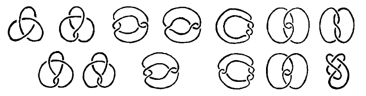
Figure 1: Knots isotopic to the trefoil knot (top row) and to the figure eight knot (bottom row)

By an isotopy of a knot we mean its continuous deformation in space as a thin elastic string; no self-intersections are allowed throughout the deformation. Two knots are isotopic if one can be transformed to the other by an isotopy.

Assertion 1.1.

(a) All the knots represented in the top row of fig. 1 are isotopic to each other. (For one pair of these knots decompose your isotopy into Reidemeister moves shown in fig. 9.)

(b) The same is true for the knots represented in the bottom row of fig. 1.

(c) All knots with the same knot diagram are isotopic.

Remark 1.2 (why a rigorous definition of isotopy is necessary?).

In fig. 2 we see an isotopy between the trefoil knot and the trivial knot.

Figure 2: A (non-ambient) isotopy between the trefoil knot and the trivial knot

Is it indeed an isotopy? This is the so called ‘piecewise linear non-ambient isotopy’, which is different from the ‘piecewise linear ambient isotopy’ defined and used later. (The first notion better reflects the idea of continuous deformation without self-intersections, but is hardly accessible to high school students, cf. [Sk16i].) In fact, any two knots are piecewise linear non-ambient isotopic!

A usual problem with intuitive definitions is not that it is hard to make them rigorous, but that this can be done in different non-equivalent ways.

A knot is a spatial closed non-self-intersecting polygonal line.

A plane diagram of a knot is its generic projection onto a plane, together with the information which part of the knot ‘goes under’ and which part ‘goes over’ at any given crossing.

Assertion 1.3.

For any knot diagram there is a knot projected to this diagram. (Such a knot need not be unique; see though assertion 1.1.c.)

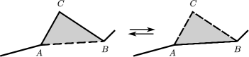
Figure 3: Elementary move

Suppose that two sides $AC$ and $CB$ of a triangle $ABC$ are edges of a knot. Moreover, assume that the knot and (the part of the plane bounded by) the triangle $ABC$ do not intersect at any other points. An elementary move $ACB\to AB$ is the replacement of the two edges $AC$ and $CB$ by the edge $AB$, or the inverse operation $AB\to ACB$ (fig. 3). Two knots $K$ and $L$ are called (piecewise linearly ambiently) isotopic if there is a sequence of knots $K_{1},\ldots,K_{n}$ such that $K_{1}=K$, $K_{n}=L$ and every subsequent knot $K_{j+1}$ is obtained from the previous one $K_{j}$ by an elementary move.

Theorem 1.4.

(a) The following knots are pairwise not isotopic: the trivial knot, the trefoil knot, the figure eight knot.

(b) There is an infinite number of pairwise non-isotopic knots.

This is proved using Arf and Casson invariants, see §5 and §9, cf. §6.

The mirror image of a knot $K$ is the knot whose diagram is obtained by changing all the crossings (fig. 8) in a diagram of $K$. By assertion 1.1.b the figure eight knot is isotopic to its mirror image.

Theorem 1.5.

The trefoil knot is not isotopic to its mirror image.

Theorem 1.5 is proved using the Jones polynomial [PS96, §3], [CDM, §2.4]. The proof is outside the scope of this text.

Theorem 1.6 (Conway–Gordon; cf. [CG83, Theorem 2]).

Take any 7 points in 3-space, no four of which belong to any plane. Take ${7\choose 2}=21$ segments joining them. Then there is a closed polygonal line formed by taken segments and non-isotopic to the boundary of a triangle.

This is proved using Arf invariant, see §5. The details are outside the scope of this text.

2 Main definitions and results on links

A link is a collection of pairwise disjoint knots, which are called the components of the link. Ordered collections are called ordered or colored links, while non-ordered collections are called non-ordered or non-colored links. In this text we abbreviate ‘ordered link’ to just ‘link’.

A trivial link (with any number of components) is a link formed by triangles in parallel planes.

Plane diagrams and isotopy for links are defined analogously to knots.

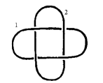
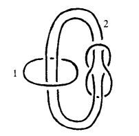
Figure 4: The Hopf link, the trivial link and another three links

Figure 5: The Borromean rings, the Whitehead link and the trefoil knot

Assertion 2.1.

(a) The Hopf link is isotopic to the link obtained from the Hopf link by switching the components.

(b) The Hopf link is isotopic to some link whose components are symmetric with respect to some straight line.

(c) The fourth link in fig. 4 is isotopic to the Whitehead link in fig. 5.w.

(d,e) The same as in (a,b) for the Whitehead link.

(f) The Borromean rings link is isotopic to a link whose components are permuted in a cyclic way under the rotation by angle $2\pi/3$ with respect to some straight line.

Proof.

(a) This follows by (b) (or can be proved independently).

(d) This follows by (e) (or can be proved independently).

Figure 6: Isotopy of the Whitehead link

(e) See figure 6.

(f) Take the quadrilaterals from figure 7, left. Then the straight line is the bisector of any octant formed by the quadrilaterals.

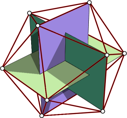
Figure 7: Borromean rings

There is also the following beautiful curvilinear construction. Take three ellipses given by the following three systems of equations:

$$\left\{\begin{array}[]{c}x=0\\ y^{2}+2z^{2}=1\end{array}\right.,\qquad\left\{\begin{array}[]{c}y=0\\ z^{2}+2x^{2}=1\end{array}\right.\qquad\text{and}\qquad\left\{\begin{array}[]{c}z=0\\ x^{2}+2y^{2}=1.\end{array}\right.$$

See figure 7, right. Then the straight line is given by $x=y=z$. ∎

Theorem 2.2.

(a) The following links are pairwise non-isotopic: the Hopf link, the trivial link, the Whitehead link.

(b) The Borromean rings link is not isotopic to the trivial link.

This is proved using linking number modulo 2, invent it yourself or see §4, and the Alexander-Conway polynomials, see §10. Alternatively, one can use the ‘triple linking’ (Massey-Milnor) number and ‘higher linking’ (Sato-Levine) number [Sk, §4.4-§4.6].

Theorem 2.3 (Conway–Gordon, Sachs; [Sk14, Theorem 1.1], cf. [CG83, Theorem 1]).

If no 4 of 6 points in 3-space lie in the same plane, then there are two linked triangles with vertices at these 6 points. That is, the part of the plane bounded by the first triangle intersects the outline of the second triangle exactly at one point.

This is proved using linking number modulo 2, see §4. The details are outside the scope of this text, see [Sk14].

3 Some basic tools

Remark 3.1 (some accurate arguments).

In the following paragraph we prove that if a knot lies in a plane, then the knot is isotopic to the trivial knot.

Denote the knot in a plane by $M_{1}M_{2}\ldots M_{n}$. Take a point $Z$ outside the plane. Then $M_{1}M_{2}\ldots M_{n}$ is transformed to the trivial knot $M_{1}ZM_{n}$ by the following sequence of elementary moves:

$$M_{1}M_{2}\to M_{1}ZM_{2},\quad ZM_{2}M_{3}\to ZM_{3},\quad ZM_{3}M_{4}\to ZM_{4},\quad\ldots,\quad ZM_{n-1}M_{n}\to ZM_{n}.$$

The following result shows that intermediate knots of an isotopy from a knot lying in a plane to the trivial knot can be chosen also to lie in this plane.

Schoenflies theorem. Any closed polygonal line without self-intersections in the plane is isotopic (in the plane) to a triangle.

This is a stronger version of the following celebrated result.

Jordan theorem. Every closed non-self-intersecting polygonal line $L$ in the plane ${\mathbb{R}}^{2}$ splits the plane into exactly two parts, i.e. ${\mathbb{R}}^{2}-L$ is not connected and is a union of two connected sets.

A subset of the plane is called connected if every two points of this subset can be connected by a polygonal line lying in this subset.

For an algorithmic explanation why the Jordan Theorem (and so the Schoenflies Theorem) is non-trivial, and for a proof of the Jordan Theorem, see §1.3 ‘Intersection number for polygonal lines in the plane’ of [Sk18], [Sk].

Assertion 3.2.

Suppose that there is a point on a knot such that if we go around the knot starting from this point, then on some plane diagram we first meet only overcrossings, and then only undercrossings. Then the knot is isotopic to the trivial knot.

Figure 8: Crossing change. The plane diagrams are identical outside the disks bounded by dashed circles. No other sides of the plane diagrams except for the pictured ones intersect the disks. (Same for fig. 9, 10, 11, 12 and 21.)

A crossing change is change of overcrossing to undercrossing or vise versa, see fig. 8.

Clearly, after any crossing change on the leftmost diagrams of the trefoil knot and the figure eight shown in fig. 1 we obtain a diagram of a knot isotopic to the trivial knot.

Lemma 3.3.

Every plane diagram of a knot can be transformed by crossing changes to a plane diagram of a knot isotopic to the trivial knot.

Figure 9: Reidemeister moves

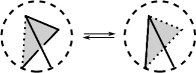
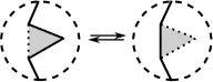
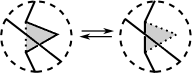
Figure 10: Left: to a rigorous definition of the first Reidemeister move
Middle, right: plane isotopy moves

In this text instead of knots up to isotopy we shall study plane diagrams of knots up to (equivalence generated by) Reidemeister moves (shown in fig. 9) and plane isotopy moves shown in fig. 10 (middle, right). I.e. we shall use without proof the following result.

Theorem 3.4 (Reidemeister).

Two knots are isotopic if and only if some plane diagram of the first knot can be obtained from some plane diagram of the second one by Reidemeister moves and plane isotopy moves.

See [PS96, §1.7]. The analogues of lemma 3.3 and theorem 3.4 for links are correct.

4 The Gauss linking number modulo 2 via plane diagrams

Suppose that there is an isotopy between two 2-component links, and the second component is fixed throughout the isotopy. Then the trace of the first component is a self-intersecting cylinder disjoint from the second component. If after the isotopy the components are unlinked, then the cylinder can be completed to a self-intersecting disk disjoint from the second component. This observation, together with [Sk, the Projection lemma 4.3.2], motivates the following definition.

The linking number modulo two $\mathop{lk}_{2}$ of the plane diagram of a 2-component link is the number modulo 2 of crossing points on the diagram at which the first component passes above the second component.

Problem 4.1.

Find the linking number modulo 2 for the plane diagrams in fig. 4 and for pairs of Borromean rings in fig. 5.b.

Lemma 4.2.

The linking number modulo 2 is preserved under Reidemeister moves.

This lemma is easily proved separately for every Reidemeister move.

By lemma 4.2 the linking number modulo 2 of a 2-component link (or even of its isotopy class) is well-defined by setting it to be the linking number modulo 2 of any plane diagram of the link.

We shall use without proof the following Parity lemma: any two closed polygonal lines in the plane whose vertices are in general position intersect at an even number of points. For a discussion and a proof see §1.3 ‘Intersection number for polygonal lines in the plane’ of [Sk18, Sk].

Assertion 4.3.

(a) Switching the components of a 2-component link preserves the linking number modulo 2.

(b) There is a 2-component link which is not isotopic to the trivial link but whose linking number modulo 2 is zero.

Part (b) is proved using integer-valued linking coefficient, see §8.

Theorem 4.4.

There is a unique mod2-valued isotopy invariant $\mathop{lk}_{2}$ of 2-component links that assumes value 0 on the trivial link and such that for any links $K_{+}$ and $K_{-}$ whose plane diagrams differ by a crossing change of a crossing $A$

$$\mathop{lk}\phantom{}_{2}K_{+}-\mathop{lk}\phantom{}_{2}K_{-}=\begin{cases}1&A\text{ is the crossing of different components;}\\ 0&A\text{ is the self-crossing of one component.}\end{cases}$$

Assertion 4.5.

If the linking number modulo 2 of two (disjoint outlines of) triangles in space is zero, then the link formed by the triangles is isotopic to the trivial link.

The proof is presumably unpublished but not hard. We encourage a reader to publish the details. Cf. [Ko19].

5 The Arf invariant

Take a plane diagram of a knot and a point $P$ on the diagram different from crossing points. Call $P$ a basepoint. A non-ordered pair of crossing points $A$ and $B$ is called skew (or $P$-skew) if going around the diagram in some direction starting from $P$ and marking only crossings at $A$ and $B$, we first mark overcrossing at $A$, then undercrossing at $B$, then undercrossing at $A$, and at last overcrossing at $B$. The $P$-Arf invariant of the plane diagram is the parity of the number of all skew pairs of crossing points.

Problem 5.1.

(a) If the $P$-Arf invariant of a plane diagram is non-zero, then $P$ is not a point as in assertion 3.2.

(b) Find the $P$-Arf invariant (of some plane diagram) of the trivial, the trefoil and the figure eight knots (for arbitrary choice of a basepoint $P$).

Lemma 5.2.

(a) The $P$-Arf invariant is independent of the choice of a basepoint $P$.

(b) The Arf invariant of a plane diagram is preserved under Reidemeister moves.

By (a) the Arf invariant of a plane diagram is well-defined by setting it to be the $P$-Arf invariant for any basepoint $P$. So the statement of (b) makes sense. By (b) the Arf invariant (Arf number) $\mathop{arf}$ of a knot (or even of isotopy class of a knot) is well-defined by setting it to be the Arf invariant of any plane diagram of the knot.

Hints. (a) It suffices to show that the Arf invariant remains unchanged when the basepoint moves through one crossing on the plane diagram.

(b) Prove the statement for each Reidemeister move separately. Cleverly choose a basepoint!

Assertion 5.3.

There is a knot which is not isotopic to the trivial knot but which has zero Arf invariant.

This is proved using Casson invariant, see §9.

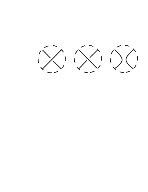
Figure 11: Links $K_{+},K_{-},K_{0}$

Theorem 5.4.

There is a unique mod2-valued isotopy invariant $\mathop{arf}$ of knots that assumes value 0 on the trivial knot and such that

$$\mathop{arf}K_{+}-\mathop{arf}K_{-}=\mathop{lk}\phantom{}_{2}K_{0}.$$

for any knots $K_{+}$ and $K_{-}$ whose plane diagrams differ as shown in fig. 11 so that $K_{0}$ is a 2-component link. (The latter is equivalent to the existence of the orientation for which fig. 11 becomes fig. 21.)

Figure 12: Pass move

Assertion 5.5.

Two knots are called pass equivalent if some plane diagram of the first knot (with some orientation) can be transformed to some plane diagram of the second knot (with some orientation) using Reidemeister moves and pass moves of fig. 12.

(a) If two knots are pass equivalent, then their Arf invariants are equal.

(b) The eight figure knot is pass equivalent to the trefoil knot.

(c) [Ka87, pp. 75–78] If the Arf invariants of two knots are equal, then the knots are pass equivalent.

6 Appendix: proper colorings

Section 6 only uses the material of §1 and §2. See more in [Pr98].

A strand in a plane diagram (of a knot or link) is a connected piece that goes from one undercrossing to the next. A proper coloring of a plane diagram (of a knot or link) is a coloring of its strands in one of three colors so that at least two colors are used, and at each crossing, either all three colors are present or only one color is present. A plane diagram (of a knot or link) is 3-colorable if it has a proper coloring.

Problem 6.1.

For each of the following knots or links take any diagram and decide if it is 3-colorable.

(a) the trivial knot.  (b) the trefoil knot.  (c) the figure eight knot.

(d-i) links in fig. 4 and 5.b.

Lemma 6.2 ([Pr95, pp. 29-30, Theorem 4.1]).

The 3-colorability of a plane diagram is preserved under the Reidemeister moves.

Theorem 6.3.

(a) Neither of links in fig. 4 and 5 (except the trivial link) is isotopic to the trivial link.

(b) The $5_{1}$ knot is not isotopic to the trivial knot.

Figure 13: The $5_{1}$ knot

7 Oriented knots and links and their connected sums

One knows what is oriented polygonal line, so one knows what is oriented knot (fig. 14).

Figure 14: Two trefoil knots with the opposite orientations

Both the informal notion and rigorous definition of isotopic oriented knots are given analogously to isotopic knots.

Assertion 7.1.

Isotopic oriented polygonal lines without self-intersections on the plane and on the sphere are defined analogously to isotopic oriented knots in space.

(a) An oriented spherical triangle is isotopic on the sphere to the same triangle with the opposite orientation.

(b) The analogue of (a) for the plane is false.

Assertion 7.2.

The following pairs of knots with opposite orientations are isotopic: two trivial knots, two trefoil knots, two figure eight knots.

Theorem 7.3 (Trotter, 1964).

There exists an oriented knot which is not isotopic to the same knot with the opposite orientation.

This is proved using the Jones polynomial [PS96, §3], [CDM, §2.4]; the proof is outside the scope of this text.

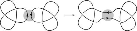
Figure 15: Connected sum of knots

The connected sum $\#$ of oriented knots is defined in fig. 15. The connected sum $\#$ of (non-oriented) knots is defined analogously (just ignore the arrows). Neither operation is well-defined on the set of knots or oriented knots, respectively. So we denote by $K\#L$ any of the connected sums of knots or oriented knots $K$ and $L$.

Assertion 7.4.

For any oriented knots $K,L,M$ and the trivial oriented knot $O$ we have

(a) $K\#O=K$.  (b) $K\#L=L\#K$.  (c) $(K\#L)\#M=K\#(L\#M)$.

(d) For any non-oriented knots $K,L$ we have $\mathop{arf}(K\#L)=\mathop{arf}K+\mathop{arf}L$.

(The rigorous meaning of (a) is ‘any connected sum of $K$ and $O$ is isotopic to $K$’. Analogous rigorous meanings have (b,c) and (d). See though remark 7.5.)

Sketch of the proof.

(a) See fig. 16.

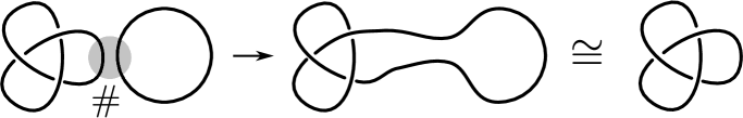
Figure 16: Proof of $K\#O=K$

Figure 17: Proofs of $K\#L=L\#K$ and of $(K\#L)\#M=K\#(L\#M)$

(b) Take a small knot isotopic to $L$ and push it through $K$, see fig. 17, left.

(c) The left hand and the right hand side of the equality are isotopic to the knot in fig. 17, right.

(d) Choose basepoint close to the ‘place of connection’. Check that all skew pairs of crossings in $K\#L$ are obtained from the skew pairs of crossings in $K$ and in $L$. ∎

Remark 7.5.

An isotopy class of a knot is the set of knots isotopic to this knot. The oriented isotopy class $[K\#L]$ of the connected sum of two oriented isotopy classes $[K],[L]$ of oriented knots $K,L$ is independent of the choices used in the construction, and of the representatives $K,L$ of $[K],[L]$. Hence the connected sum of oriented isotopy classes of oriented knots is well-defined by $[K]\#[L]:=[K\#L]$, see [Sk15, Remark 2.3.a]. For isotopy classes of non-oriented knots the connected sum is not well-defined [CSK].

Theorem 7.6.

For any isotopy classes $K,L,M$ of knots and the isotopy class $O$ of the trivial oriented knot we have

(a) if $K\#L=O$, then $K=L=O$;

(b) if $K\#L=K\#M$, then $L=M$.

The proof is outside the scope of this text, see [PS96, Theorem 1.5]. (In this part of [PS96] one needs to replace ‘knot’ by ‘oriented knot’ because of remark 7.5.)

Figure 18: Connected sum of links

The connected sum $\#$ of links (ordered or not, oriented or not) is defined analogously to the connected sum of knots, see fig. 18. This is not a well-defined operation on links, and assertion 7.8 shows that this does not give a well-defined operation on their isotopy classes. So we denote by $K\#L$ any of the connected sums of $K$ and $L$.

Assertion 7.7.

(a,b,c) The analogues of assertions 7.4.a,b,c for links are true.

(b) For any non-oriented 2-component links $K,L$ we have $\mathop{lk}_{2}(K\#L)=\mathop{lk}_{2}K+\mathop{lk}_{2}L$.

Figure 19: Connected sum of isotopy classes of ordered links is not well-defined

Remark 7.8.

There are two isotopic pairs $(K,L)$ and $(K^{\prime},L^{\prime})$ of 2-component links such that some connected sums $K\#L$ and $K^{\prime}\#L^{\prime}$ are not isotopic. (The links could be ordered or non-ordered, oriented or non-oriented, so that we have 4 statements.) As an example of non-ordered pairs we can take equal links consisting of a trefoil and an unknot in disjoint cubes, cf. [PS96, Figure 3.16]. For an example of ordered pairs see [As]. Fig. 19 presents an alternative example suggested by A. Ryabichev.

8 The Gauss linking number via plane diagrams

Let $(\overrightarrow{AB},\overrightarrow{CD})$ be an ordered pair of vectors (oriented segments) in the plane intersecting at a point $P$. Define the sign of the pair to be $+1$ if $ABC$ is oriented clockwise and to be $-1$ otherwise (fig. 20).

Figure 20: The sign of intersection point

The linking number $\mathop{lk}$ of the plane diagram of an oriented 2-component link is the sum of signs at all those crossing points on the diagram at which the first component passes above the second component. At every crossing point the first (the second) vector is the oriented edge of the first (the second) component.

Problem 8.1.

Find the linking number for (some plane diagram of) the Hopf link and pairs of Borromean rings, for your choice of orientation on the components.

Lemma 8.2.

The linking number is preserved under Reidemeister moves.

The proof is analogous to lemma 4.2. It suffices to check that the signs of all crossing points do not change.

By Lemma 8.2 the linking number of an oriented 2-component link (or of its isotopy class) is well-defined by setting it to be the linking number of any plane diagram of the link.

The absolute value of the linking number of a (non-oriented) 2-component link (or of its isotopy class) is well-defined by taking any orientations on the components.

We shall use without proof the following Triviality lemma: for any two closed oriented polygonal lines in the plane whose vertices are in general position the sum of signs of their intersection points is zero. For a discussion and a proof see §1.3 ‘Intersection number for polygonal lines in the plane’ of [Sk18], [Sk].

Assertion 8.3.

(a) Switching the components of a link negates the linking number.

(b) Reversing the orientation of either of the components negates the linking number.

(c) There is an oriented 2-component link whose linking number is $-5$.

(d) For any of the connected sums $K\#L$ of oriented 2-component links $K,L$ we have $\mathop{lk}(K\#L)=\mathop{lk}K+\mathop{lk}L$.

(e) There is a 2-component link which is not isotopic to the trivial link but which has zero linking number.

Part (e) is proved using Alexander-Conway polynomial, see §10.

Theorem 8.4.

There is a unique integer-valued isotopy invariant $\mathop{lk}$ of oriented 2-component links that assumes value 0 on the trivial link and such that for any links $K_{+}$ and $K_{-}$ whose plane diagrams differ by a crossing change of a crossing $A$ as shown in fig. 21

$$\mathop{lk}K_{+}-\mathop{lk}K_{-}=\begin{cases}1&A\text{ is the crossing of different components;}\\ 0&A\text{ is the self-crossing of one component.}\end{cases}$$

The proof is analogous to theorem 4.4.

Figure 21: Oriented links $K_{+},K_{-},K_{0}$

9 The Casson invariant

The sign of a crossing point of an oriented plane diagram of a knot is defined after figure 20; the first (the second) vector is the vector of overcrossing (of undercrossing). Clearly, the sign is independent of the orientation of the diagram, and so is defined for non-oriented diagram.

The sign of a $P$-skew pair of crossing points in a plane diagram of a knot (for any basepoint $P$) is the product of the signs of the two crossing points.

The $P$-Casson invariant of a plane diagram is the sum of signs over all $P$-skew pairs of crossing points.

Problem 9.1.

(a) Same as problem 5.1.b for the Casson invariant.

(b) Draw a plane diagram of a knot and a basepoint $P$ such that $P$-Casson invariant is $-5$.

Lemma 9.2.

(a,b) Same as lemma 5.2.a,b for the Casson invariant.

Hence the Casson invariant (number) $c_{2}$ of a plane diagram, of a knot, or even of isotopy class of a knot, is well-defined by setting it to be the $P$-Casson invariant of any plane diagram of the knot for any basepoint $P$.

Assertion 9.3.

(a,b) Same as assertions 7.4.d and 5.3 for the Casson invariant.

Part (b) is proved using Alexander-Conway polynomial, see §10.

Denote by $D_{+},D_{-},D_{0}$ any three diagrams of oriented (knots or) links differing as shown in fig. 21 (for a convention on figures see caption to fig. 8). We also denote by $K_{+},K_{-},K_{0}$ any three links who have diagrams $D_{+},D_{-},D_{0}$.

Theorem 9.4.

There is a unique integer-valued isotopy invariant $c_{2}$ of (non-oriented) knots that assumes value 0 on the trivial knot and such that for any knots $K_{+}$ and $K_{-}$ whose plane diagrams differ as shown in fig. 21

$$c_{2}(K_{+})-c_{2}(K_{-})=\mathop{lk}K_{0}.$$

(Observe that $K_{0}$ has to be a 2-component link; the number $\mathop{lk}K_{0}$ is well-defined because change of the orientation on both components of an oriented link does not change the linking number.)

10 Alexander-Conway polynomial

Section 10 only uses the material of §1, §2 and §7 (except that assertions 10.4.bc use §8 and §9).

Problem 10.1.

(a) There is a unique mod2-valued isotopy invariant $\mathop{arf}$ of oriented 3-component links that assumes value 0 on the trivial link and for which

$$\mathop{arf}K_{+}-\mathop{arf}K_{-}=\begin{cases}\mathop{lk}\phantom{}_{2}K_{0}&\text{at the crossing point different components cross each other;}\\ 0&\text{at the crossing point one component crosses itself.}\end{cases}$$

(Here $\mathop{lk}_{2}K_{0}$ is defined because $K_{0}$ is a 2-component link.)

(b) Assuming the existence of the invariant $\mathop{arf}$ from (a), calculate (for your choice of orientation on the components) the $\mathop{arf}$ invariant of the Borromean rings.

Theorem 10.2.

There is a unique infinite sequence $c_{-1}=0,c_{0},c_{1},c_{2},\ldots$ of ${\mathbb{Z}}$-valued isotopy invariants of oriented non-ordered links such that

$\bullet$ $c_{0}=1$ and $c_{1}=c_{2}=\ldots=0$ for the trivial knot;

$\bullet$ for any $n\geq 0$ and links $K_{+},K_{-},K_{0}$ from fig. 21 we have

$$c_{n}(K_{+})-c_{n}(K_{-})=c_{n-1}(K_{0}).$$

Proofs of the existence in assertion 10.1.a and in theorem 10.2 are outside the scope of this text. We shall use the existence without proof. See a proof in [Al28], [Ka06’, §3-§5], [Ka06], [Ma18, §5.5 and §5.6], [Ga20]. For a relation to proper colorings see [Ka06’, §6].

The polynomial $C(K)(t):=c_{0}(K)+c_{1}(K)t+c_{2}(K)t^{2}+\ldots$ is called the Conway polynomial, see assertion 10.4.e. Introduction of this polynomial allows to calculate all the invariants $c_{n}$ as quickly as one of them. The formula in theorem 10.2 is equivalent to

$$C(K_{+})-C(K_{-})=tC(K_{0}).$$

Problem 10.3.

Calculate the Conway polynomial of the following links (for your choice of orientation on the components).

(a) the trivial link with 2 components;  (b) the trivial link with $n$ components;

(c) the Hopf link;  (d) the trefoil knot;  (e) the figure eight knot;

(f) the Whitehead link;  (g) the Borromean rings;  (h) the $5_{1}$ knot.

Assertion 10.4.

(a) We have $c_{0}(K)=1$ if $K$ is a knot and $c_{0}(K)=0$ otherwise (i.e. if $K$ has more than one component).

(b) For a knot $K$ we have $c_{2j+1}(K)=0$ and $c_{2}$ is the Casson invariant.

(c) For a 2-component link $K$ we have $c_{2j}(K)=0$ and $c_{1}$ is the linking coefficient.

(d) For a $k$-component link $K$ we have $c_{j}(K)=0$ if either $j\leq k-2$ or $j-k$ is even.

(e) For every knot or link all but a finitely many of the invariants $c_{n}$ are zeroes.

Assertion 10.5.

(a) Change of the orientations of all components of a link (in particular, change of the orientation of a knot) preserves the Conway polynomial.

(b) [CDM, 2.3.4] There is a 2-component link such that change of the orientation of its one component changes the degree of the Conway polynomial (so this change neither preserves nor negates the Conway polynomial).

(c) For any of the connected sums $K\#L$ of knots $K,L$ we have $C(K\#L)=C(K)C(L)$.

Assertion 10.6.

A link is split if it is isotopic to a link whose components are contained in disjoint balls.

(a) Neither Hopf link nor Whitehead link nor Borromean rings link is split.

(b) The linking coefficient of a split link is zero.

(c) The Conway polynomial of a split link is zero.

11 Vassiliev-Goussarov invariants

Section 11 only uses the material of §1, §2 and §7 (except that problem 11.3.2 uses §9).

An (oriented) singular knot is a closed oriented polygonal line in ${\mathbb{R}}^{3}$ whose only self-intersections are double points which are not vertices. Two singular knots are isotopic if there is an orientation preserving PL homeomorphism $h:{\mathbb{R}}^{3}\to{\mathbb{R}}^{3}$ carrying the first singular knot to the second one, and the orientation on the first singular knot to the orientation on the second one. Denote by $\Sigma$ the set of all isotopy classes of singular knots.

A chord diagram is a cyclic word of length $2n$ having $n$ letters, each letter appearing twice. A chord diagram is depicted as an oriented circle with a collection of chords, cf. [Sk20, §1.5]. For a singular knot $K$ denote by $\sigma(K)$ the following chord diagram. Move uniformly along the oriented circle and for any point $A$ on the circle take the ‘corresponding’ point $f(A)$ on $K$. Join by a chord each pair of points on the circle corresponding to the intersection point of $K$ [PS96, 4.8], [CDM, 3.4.1].

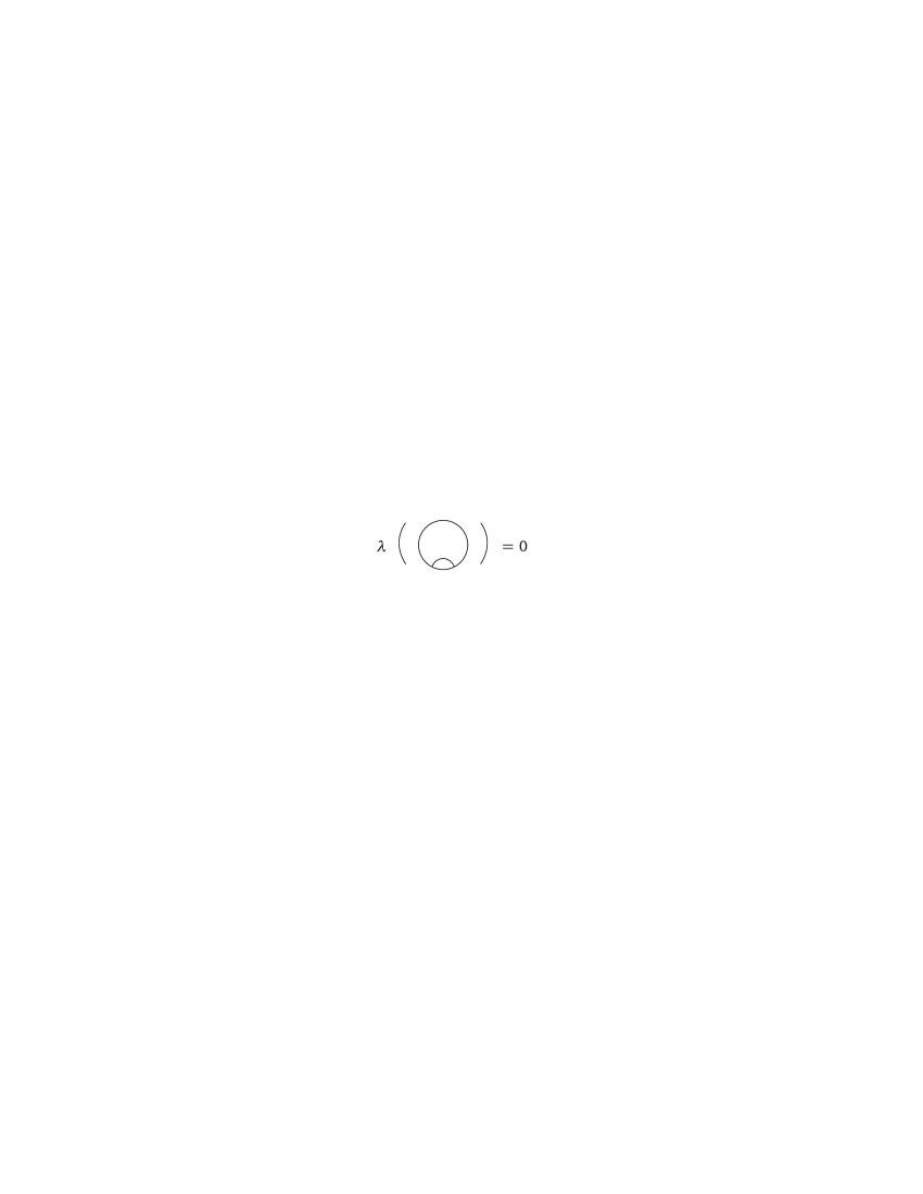
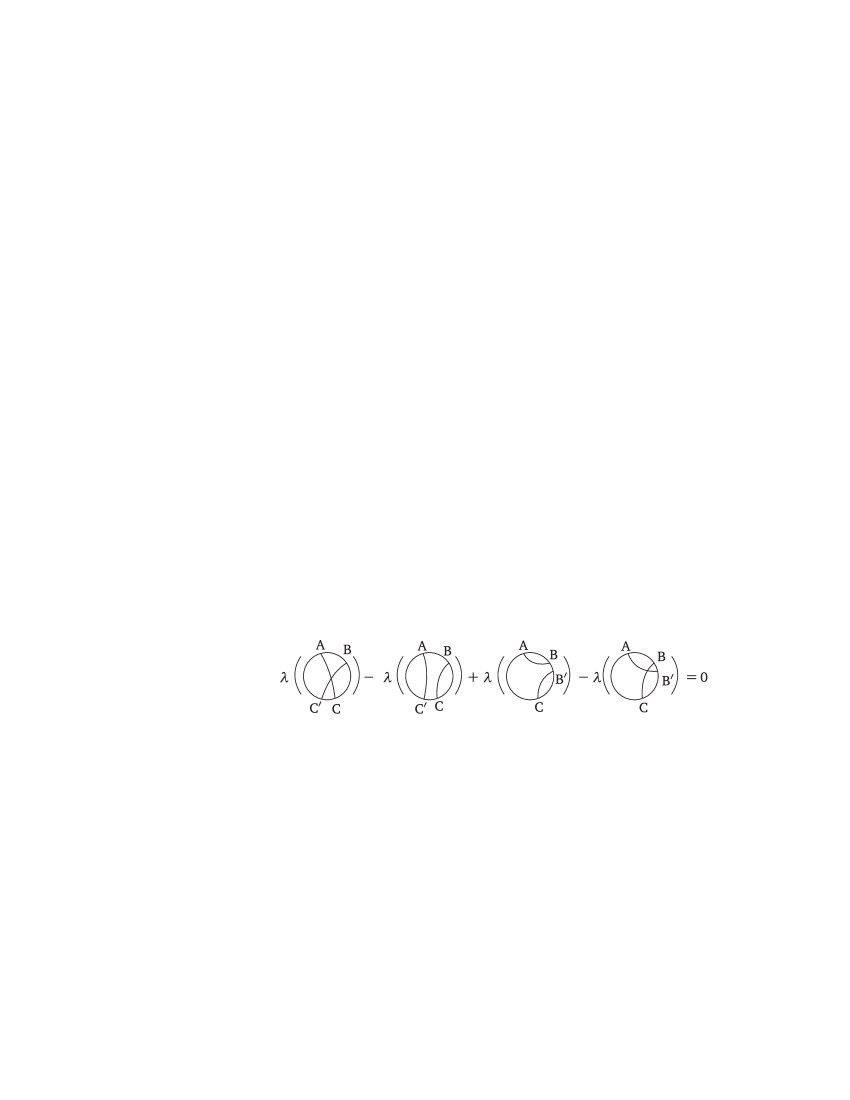
Figure 22: The 1-term and 4-term relations

Theorem 11.1.

Assume that $n\geq 0$ is an integer and $\lambda:\delta_{n}\to{\mathbb{R}}$ a map from the set $\delta_{n}$ of all chord diagrams that have $n$ chords. The map $\lambda$ satisfies the 1-term and the 4-term relations from fig. 22 if and only if there exists a map $v:\Sigma\to{\mathbb{R}}$ (i.e. an invariant of singular knots) such that

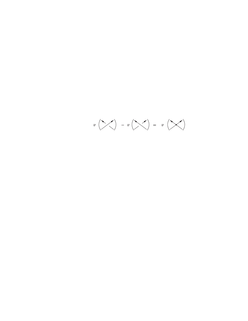
Figure 23: The Vassiliev skein relation, notice the difference with fig. 21

(1) The Vassiliev skein relation from fig. 23 holds,

($2_{n}$) $v(K)=0$ for each singular knot that has more than $n$ self-intersection points, and

(3) $v(K)=\lambda(\sigma(K))$ for each singular knot $K$ that has exactly $n$ self-intersection points.

The proof is outside the scope of this text.

As far as I know, the Vassiliev-Kontsevich theorem 11.1 was never stated in this form, which is short and convenient for calculation of the invariants (although this form was implicitly used when the invariants were calculated). I am grateful to S. Chmutov for confirmation that theorem 11.1 is correct and is indeed equivalent to the standard formulation of the Vassiliev-Kontsevich theorem, see e.g. [CDM, Theorem 4.2.1], cf. [PS96, Theorem 4.12].

A map $v:\Sigma\to{\mathbb{R}}$ such that (1) holds is called a Vassiliev-Goussarov invariant. If additionally ($2_{n}$) holds, then $v$ is called a invariant of order at most $n$. The following assertion shows that the map $v$ of theorem 11.1 is unique up to Vassiliev-Goussarov invariant of order at most $n-1$.

Assertion 11.2 ([CDM, Proposition 3.4.2]).

The difference between maps $v,v^{\prime}:\Sigma\to{\mathbb{R}}$ satisfying to (1), ($2_{n}$) and (3), satisfies to (1) and ($2_{n-1}$).

Problem 11.3.

(a) Prove the ‘if’ part of theorem 11.1.

(0),(1),(2) Prove the ‘only if’ part of theorem 11.1 for $n=0,1,2$.

Hint. For $n=2$ use theorem 9.4.

(The ‘only if’ part of theorem 11.1 for $n=3$ could be proved using the coefficient of $h^{3}$ in $J(e^{h})$, where $J$ is the Jones polynomial in $t$-parametrization [CDM, 2.4.2, 2.4.3] [PS96, (4.6)].)

In the remaining problems use (the ‘only if’ part of) theorem 11.1 without proof. Assertion ‘$v(K)=x$ for any singular knot $K$ whose chord diagram is $A$’ is shortened to ‘$v(A)=x$’.

Problem 11.4.

(a) There exists a unique Vassiliev-Goussarov invariant $v_{2}:\Sigma\to{\mathbb{R}}$ of order at most 2 such that $v_{2}(O)=0$ for the trivial knot $O$ and $v_{2}(1212)=1$. (Here (1212) is the ‘non-trivial’ chord diagram with 2 chords, see [PS96, Figure 4.4], 3rd diagram of the first line.)

Hint. This follows from theorem 9.4, but try to deduce this from theorem 11.1.

(b,b’,c,d) Calculate $v_{2}$ for the (arbitrary oriented) right trefoil, left trefoil, figure eight knot and the $5_{1}$ knot.

Problem 11.5.

(a) There exists a unique Vassiliev-Goussarov invariant $v_{3}:\Sigma\to{\mathbb{R}}$ of order at most 3 such that $v_{3}(O)=0$ for the trivial knot $O$ and for the left trefoil $O$, and $v_{3}(123123)=1$. (Here (123123) is the ‘non-trivial most symmetric chord diagram with 3 chords’, see [PS96, Figure 4.4], 5th diagram of the second line.)

(b,b’,c,d) Same as problem 11.4 for $v_{3}$.

Hints. See Problems 2, 3, 4ab, Results/Theorems 11, 13, 14 from [PS96, §4].

Problem 11.6.

(a) [PS96, Problem 4.4.b] There exists a unique Vassiliev-Goussarov invariant $v_{4}:\Sigma\to{\mathbb{R}}$ of order at most 4 such that

$\bullet$ $v_{4}(O)=0$ for the trivial knot $O$, for the left trefoil $O$, and for the right trefoil $O$,

$\bullet$ $v_{4}(12341234)=2$, $v_{4}(12341432)=3$ and $v_{4}(12341423)=5$.

(b,b’,c,d) Same as problem 11.4 for $v_{4}$.

12 Appendix: some details

1.1. (a,b) ‘Probably the best way of solving this problem is to make a model of the trefoil knot and the figure eight knot by using a shoelace and then move it around from one position to the other. Fig. 24 gives some hints concerning transformations of the trefoil and the figure eight knot.’ [Pr95, §2] (Fig. 24, left, is prepared by D. Kroo.)

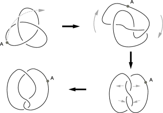
Figure 24: Isotopy the trefoil and of the figure eight knot

(e) Consider two knots with coinciding plane diagrams in a ‘horizontal’ plane $\pi$. For each point $X$ in the space let $p(X)$ be the line containing $X$, perpendicular to $\pi$. Let $h(X)$ be the height of $X$ relative to $\pi$, that is positive ($h(X)>0$) if $X$ is in the upper half-space, and is negative ($h(X)<0$) if $X$ is in the lower half-space. To each point $A$ of the first knot associate a point $A^{\prime}$ of the second knot by the following procedure.

Case 1: The projection of the point $A$ on $\pi$ is not a crossing point on the plane diagram. In this case $p(A)$ intersects the first knot only at the point $A$. Since the plane diagrams coincide, the line $p(A)$ intersects the second knot also at a single point. Define $A^{\prime}$ to be this point.

Case 2: The projection of the point $A$ on $\pi$ is a crossing point of the plane diagram. In this case the line $p(A)$ intersects the first knot in an additional point $B$. Since the plane diagrams coincide, the line $p(A)$ intersects the second knot in two points $C$ and $D$, where we assume that $h(C)>h(D)$. If $h(A)>h(B)$, we define $A^{\prime}=C$, and in the opposite case $A^{\prime}=D$.

For each point $A$ of the first knot and each number $t\in[0,1]$ let $A(t)$ be the point on the line $p(A)$ with the height $h(A(t))=(1-t)h(A)+th(A^{\prime})$. By construction $A(0)=A$, $A(1)=A^{\prime}$ and the transformation of the first knot, which moves $A(0)$ in the direction of $A(1)$ with constant speed, so that at the time $t$ it occupies the position $A(t)$, is the required isotopy.

Figure 25: The bridge over some crossing point

1.3. See fig. 25. For each crossing point of the plane diagram, on the upper edge of the crossing, choose two points, close to the intersection and on the opposite sides of the intersection. Replace the line segment between the two chosen points by a ‘bridge’ rising above the plane diagram, which connects these two points. After replacing all crossing points by the corresponding bridges, we obtain the required knot.

1.4. (a) Use the results of problems 5.1.b, 9.1.a and lemmas 5.2.ab, 9.2.ab. Alternatively, use the results of problem 6.1.ab and lemma 6.2.

(b) Take any of the connected sums of $n$ trefoil knots. By the results of problems 9.1.a and 9.3.a the Casson invariant of this knot is $n$. Hence by lemma 9.2.ab these knots for different values of $n$ are not isotopic.

2.2. (a) In order to distinguish the Hopf link from the other two use the result of problem 4.1 and lemma 4.2. In order to distinguish the Whitehead link from the trivial link use the result of problem 6.1 (or 10.3) and lemma 6.2 (or theorem 10.2).

(b) Use the result of problem 10.3 and theorem 10.2.

3.2. Choose a knot projected to the given plane diagram in the same way as in assertion 1.3. Suppose that all the ‘bridges’ lie in the upper half-space w.r.t. the projection plane. By the assumption there are points $X$ and $Y$ on the knot which divide the knot into two polygonal lines $p$ and $q$ such that

$\bullet$ $q$ lies in the projection plane and passes only through undercrossings;

$\bullet$ $p$ is projected to polygonal line $p^{\prime}$ which passes only through overcrossings.

Take a point $Z$ in the upper half-space, and a point $T$ in the lower half-space. Let us construct an isotopy between the given knot and the closed polygonal line $XZYT$, which is isotopic to the trivial knot. The isotopy consists of 3 steps, all of them keeping $X,Y$ fixed.

Step 1. An isotopy between $q$ and $XTY$. Suppose that $q=A_{0}A_{1}\ldots A_{n}$, where $A_{0}=X$ and $A_{n}=Y$. Then the isotopy is given by

$$A_{0}A_{1}\to A_{0}TA_{1},\quad TA_{1}A_{2}\to TA_{2},\quad TA_{2}A_{3}\to TA_{3},\quad\ldots TA_{n-1}A_{n}\to TA_{n}.$$

Step 2. An isotopy between $p$ and $p^{\prime}$. Remove all the ‘bridges’ by elementary moves.

Step 3. An isotopy between $p^{\prime}$ and $XZY$. This is done analogously to step 1.

3.3. Follows by assertion 3.2.

Another idea of the proof (cf. [PS96, Theorem 3.8]). Denote by $\pi$ the horizontal plane containing the plane diagram. For each point $X$ in the space, $p(X)$ and $h(X)$ are defined in the solution of the problem 1.1.c. Let $l$ be a line in the plane, which passes through a vertex $A_{0}$ of the plane diagram, while the whole diagram is contained in one of the two half-planes determined by $l$. Let $A_{0},A_{1},\ldots A_{n}$ be all vertices of the plane diagram, in the order of their appearance, while we move along the diagram in some direction. Choose points $B_{0},\ldots,B_{n}$ so that $A_{i}\in p(B_{i})$ for $i=1,\ldots,n$, and $h(B_{i})<h(B_{j})$ for $i<j$. Let $B_{n+1}$ be a point, whose projection on $\pi$ is close to $A_{0}$ and $h(B_{n+1})>h(B_{n})$. We claim that the knot $B_{0}\ldots B_{n}B_{n+1}$ is isotopic to the trivial knot. Indeed, by the choice of the line $l$, the projection of the knot onto any plane, perpendicular to the line $l$, is a closed polygonal line without self-intersections. It remains to modify crossing in the plane diagram so that they are in agreement with the projection of the constructed knot to the plane $\pi$.

4.1. Answer: 1 for the Hopf link and 0 for other links.

4.2. For moves I and III the number of crossing points where the first component passes above the second one does not change. For move II this number changes by $0$ or $\pm 2$.

4.3. (a) Take a plane diagram of a link. By the Parity lemma stated before assertion 4.3 the number of crossing points where the first component passes above the second one has the same parity as the number of crossing points where the second component passes above the first one. This is the required statement.

(b) An example is the third link in fig. 4. This link is not isotopic to the trivial link because they have distinct linking numbers, see §8.

4.4. Existence. By lemma 4.2 the linking number modulo 2 is an isotopy invariant. The skein relation is easy to check.

Uniqueness. Suppose that $\mathrm{f}$ is another invariant aside from $\mathop{lk}_{2}$ satisfying the assumptions. Then $\mathrm{f}-\mathop{lk}_{2}$ is an isotopy invariant assuming zero value on the trivial link and invariant under crossing changes. The analogue of lemma 3.3 for links states that any plane diagram of a link can be obtained from the diagram of a link isotopic to the trivial link by some crossing changes. Hence $\mathrm{f}-\mathop{lk}_{2}=0$.

5.1. (a) If $P$ is a point on the plane diagram as in assertion 3.2, then there are no $P$-skew pairs of crossings. Hence the $P$-Arf invariant is zero.

5.2. (a) Let $P_{1}$ and $P_{2}$ be two basepoints such that the segment $P_{1}P_{2}$ contains exactly one crossing point $X$.

Case 1: $P_{1}P_{2}$ passes through undercrossing. Then $X$ does not form either $P_{1}$-skew or $P_{2}$-skew pair with any other crossing. Hence $P_{1}$- and $P_{2}$-Arf invariants of the diagram are equal.

Case 2: $P_{1}P_{2}$ passes through overcrossing. Then $X$ divides the diagram into two closed polygonal lines $q_{1}$ and $q_{2}$ such that $P_{1}$ lies on $q_{1}$ and $P_{2}$ lies on $q_{2}$. Denote by $n_{1}$ (respectively, $n_{2}$) the number of intersections of $q_{1}$ and $q_{2}$ for which $q_{1}$ passes above $q_{2}$ (respectively, $q_{2}$ passes above $q_{1}$). Denote by $N_{1}$ the number of $P_{1}$-skew pairs formed by $X$ and some intersection of $q_{1}$ and $q_{2}$. Denote by $\mathop{arf}_{P_{1}}D$ the $P_{1}$-arf invariant of $D$. Use analogous notation with $P_{1}$ replaced by $P_{2}$. Then

$${\mathop{arf}}_{P_{1}}D-{\mathop{arf}}_{P_{2}}D=N_{1}-N_{2}=n_{1}-n_{2}\underset{2}{\equiv}n_{1}+n_{2}\underset{2}{\equiv}0,$$

where $D$ is the given plane diagram. Here

$\bullet$ the first equality holds because a pair of crossings is either $P_{1}$-skew or $P_{2}$-skew (but not both) if and only if the pair is formed by $X$ and some intersection of $q_{1}$ and $q_{2}$;

$\bullet$ the second equality holds because $N_{1}=n_{1}$ and $N_{2}=n_{2}$; indeed, an intersection of $q_{1}$ and $q_{2}$ forms a $P_{1}$-skew (respectively, $P_{2}$-skew) pair with $X$ if and only if at this intersection $q_{1}$ passes above (respectively, below) $q_{2}$;

$\bullet$ $\underset{2}{\equiv}$ are congruences modulo 2;

$\bullet$ the last congruence follows by the Parity lemma for $q_{1}$ and $q_{2}$.

Figure 26: Arf-invariant does not change under Reidemeister moves

(b) Type $I$ move. Take basepoints before and after the move as in fig. 26 (left). Check that the crossing $A$ does not form a $P$-skew pair with any other crossing.

Type $II$ move. Take basepoints before and after the move as in fig. 26 (middle). Check that neither of the crossings $A$ and $B$ forms a $P$-skew pair with any other crossing.

Type $III$ move. Take basepoints before and after the move as in fig. 26 (right). Check that neither of the crossings $A$, $B$ forms a $P$-skew pair with any other crossing and that neither of the crossings $A^{\prime}$, $B^{\prime}$ forms a $P^{\prime}$-skew pair with any other crossing. Then check that a crossing $X$ distinct from $A$, $B$, $C$ forms a $P$-skew pair with $C$ if and only if $X$ forms a $P^{\prime}$-skew pair with $C^{\prime}$.

5.3. Take any connected sum $K$ of the two trefoil knots. By assertion 7.4.d $\mathop{arf}K=0$. By the result of problem 9.1.b and assertion 9.3.a $c_{2}(K)\neq 0$. Hence $K$ is not isotopic to the trivial knot.

Figure 27: To the proof of skein relation for Arf invariant

5.4. Existence. By lemma 5.2, the arf invariant is an isotopy invariant. Here are hints for checking the skein relation. Take basepoints $P_{+}$, $P_{-}$ as in fig. 27. Check that the crossing $A_{-}$ does not form a $P_{-}$-skew pair with any other crossing in $K_{-}$. Then check that the number of crossings which form a $P_{+}$-skew pair with $A_{+}$ in $K_{+}$ equals $\mathop{lk}\phantom{}_{2}K_{0}$ modulo 2.

Uniqueness. The proof is analogous to the proof of theorem 4.4. Use lemma 3.3 itself instead of its analogue for links.

Figure 28: A 3-coloring of a link and a 5-coloring of the $5_{1}$ knot

6.1. Answers: b,e,h — 3-colorable, a,c,d,f,g,i — not 3-colorable. For a proper coloring of a diagram of trefoil knot see [Pr95, p. 30, figure 4.3]. For a proper coloring of the last diagram from fig. 4 see fig. 28 left. (This diagram was erroneously stated to be not 3-colorable in [Pr95, §4]. This minor mistake was found by L.M. Bannöhr, S. Zotova and L. Kravtsova.)

6.3. (a) Most part of (a) follows by lemma 6.2 and results of problems 6.1.d-h (see [Pr95, p. 30]). The last diagram from fig. 4 is distinguished from the trivial link by the number of proper colorings of a plane diagram. Prove that this number is preserved under the Reidemeister moves.

(b) A plane diagram is 5-colorable if there exists a coloring of its strands in five colors $0,1,2,3,4$ so that at least two colors are used, and at each crossing if the upper strand has color $a$ and two lower strands have colors $b$ and $c$, then $2a\equiv b+c\pmod{5}$. Similarly to lemma 6.2 the 5-colorability of a plane diagram is preserved under Redemeister moves. The $5_{1}$ knot is 5-colorable, see fig. 28, right. The trivial knot is not. Hence they are not isotopic.

7.1. (b) First solution. An oriented polygonal line is called positive if the bounded part of the plane is always on the left side of each of its oriented segments (see the Jordan theorem in remark 3.1). Prove that the positivity of an oriented polygonal line is preserved by elementary moves.

Hint to the second solution. The positivity can be equivalently defined as follows. We say that an oriented polygonal line $A_{1}\ldots A_{n}$ is positive if for each of its inner (interior) points $O$ the sum of oriented angles $\angle A_{1}OA_{2}+\angle A_{2}OA_{3}+\ldots+\angle A_{n-1}OA_{n}+\angle A_{n}OA_{1}$ is always positive (i.e. the winding number of the oriented polygonal line around any interior point is positive).

7.2. Each of the three indicated oriented knots is transformed into the oriented knot with the opposite orientation by the rotation through the angle $\pi$ around the ‘vertical’ axis passing through the ‘upper’ point of the knot (see the leftmost diagram in fig. 1, the first and the second row for the trefoil and the figure eight knot, respectively). This rotation is included into a continuous family of rotations through the angle $\pi t$, $t\in[0,1]$, with respect to the same line. This is the required isotopy.

7.7. (d) Check that all crossings of different components in $K\#L$ are obtained from such crossings in $K$ and in $L$.

8.1. Answers: $\pm 1$; 0.

8.3. (a) The proof is analogous to assertion 4.3.a. Take a plane diagram of a link. By the Triviality lemma (stated before assertion 8.3) the sum of signs of crossing points where the first component passes above the second one has opposite sign to the sum of signs of crossing points where the second component passes above the first one. Switching the components negates the sign of every crossing point. This completes the proof.

(b) Reversing the orientation of either of the components negates the sign of every crossing point.

(c) Take the connected sum of 5 Hopf links oriented so that their linking numbers equal to $-1$.

(d) The proof is analogous to assertion 7.4.d. The signed set of crossing points of plane diagram of $K\#L$ is the union of the signed sets of crossing points of plane diagrams of links $K$ and $L$.

(e) An example is the Whitehead link. The Whitehead link is not isotopic to the trivial link by theorem 2.2.a.

9.1. (a) Answers: 0, 1 and $-1$.

The trivial knot has no crossings, and so no skew pairs of crossings. Therefore the Casson invariant of this knot is 0.

All three crossings of the trefoil knot have the same sign. Since the trefoil knot has exactly one linked pair of crossings (regardless the choice of the base-point), we obtain that the Casson invariant of this knot is 1.

(b) Take any connected sum of five figure eight knots. By (a) and assertion 9.3.a below the Casson invariant of this knot is $-5$.

9.2, 9.3.a, 9.4. The proofs are analogous to lemma 5.2, assertion 5.3 and theorem 5.4, respectively. Take care of the signs of intersection points. For lemma 9.2.a use the Triviality lemma stated before assertion 8.3.

9.3. (b) Take any connected sum of the trefoil knot and the figure eight knot. By (a) and the answer to problem 9.1.a the Casson invariant of this knot is 0. However, by the answers to problems 10.3.d,e and assertion 10.5.c the Conway polynomial of this knot is $(1+t^{2})(1-t^{2})\neq 1$. Hence this knot is not isotopic to the trivial knot.

10.1. (b) Answer: 0.

Remark. The invariant $\mathop{arf}=c_{2}\mod 2$ for links may depend on the orientation on the components (for $c_{3}\mod 2$ see [CDM, 2.3.4]).

Let $D$ be a plane diagram of a link. Denote by $\mathrm{cr}D$ the number of crossings in $D$. Denote by $\mathrm{ch}D$ the minimal number of crossing changes required to obtain from $D$ a diagram of a link which is isotopic to the trivial one (such sequence of crossing changes exists by the analogue of lemma 3.3 for links).

10.2. The uniqueness is analogous to theorems 8.4,9.4; solve first problem 10.3.

Deduction of the stronger version (for non-ordered links) from the weaker version (for ordered links). It suffices to show that all invariants $c_{n}$ defined for ordered links are preserved under changes of the order of the components.

Let $D$ be a plane diagram of a link with two or more components and let $D^{\prime}$ be a plane diagram obtained from $D$ by a change of the components’ order. The proof is by induction on $\mathrm{cr}D$. If $\mathrm{cr}D=0$, then $D$ is a diagram of a link which is isotopic to the trivial one and by the answer to problem 10.3.b we have $C(D)=0$ for any ordering of the components. Suppose that $\mathrm{cr}\,D>0$; then continue the proof by induction on $\mathrm{ch}D$. If $\mathrm{ch}D=0$, then $D$ is a diagram of a link which is isotopic to the trivial one; this case is considered above. Suppose that $\mathrm{ch}D>0$. Let $D_{*}$ be a link obtained from $D$ by a crossing change and such that $\mathrm{ch}D_{*}<\mathrm{ch}D$. Denote by $D^{\prime}_{*}$ is a link obtained from $D^{\prime}$ by the change of the same crossing. Then

$$\pm(C(D)-C(D_{*}))=C(D_{0})\quad\mbox{and}\quad\pm(C(D^{\prime})-C(D^{\prime}_{*}))=C(D^{\prime}_{0}),$$

where $D_{0}$ is a diagram of a link $K_{0}$ (with some ordering of the components) from fig. 21 for $D$, $D_{*}$ being $D_{+}$, $D_{-}$ in some order, and $D^{\prime}_{0}$ is the same for $D^{\prime}$, $D^{\prime}_{*}$. Note that the diagrams $D_{*}$ and $D^{\prime}_{*}$ coincide up to the order of the components. The same is true for the diagrams $D_{0}$ and $D^{\prime}_{0}$. Since $\mathrm{ch}D_{*}<\mathrm{ch}D$ and $\mathrm{cr}\,D_{0}<\mathrm{cr}\,D$, by the inductive hypotheses we have $C(D_{*})=C(D^{\prime}_{*})$ and $C(D_{0})=C(D^{\prime}_{0})$. Then $C(D)=C(D^{\prime})$.

10.3. Answers: (a, b) 0; (c) $\pm t$; (d) $1+t^{2}$; (e) $1-t^{2}$; (f) $\pm t^{3}$; (g) $\pm t^{4}$; (h) $1+3t^{2}+t^{4}$.

Remark. The signs in the answers to (c), (f), (g) depend on the orientation on the components.

Hint. For examples of such calculations for (a), (c), and (d) see [CDM, 2.3.2].

10.4. Let $D$ be a plane diagram of the given link $K$.

(a) For any diagram $D_{*}$ obtained from $D$ by a crossing change we have $c_{0}(D)-c_{0}(D_{*})=0$, i. e. $c_{0}$ does not change under crossing changes. By the analogue of lemma 3.3 for links the diagram $D$ can be obtained by crossing changes from a diagram of a link isotopic to the trivial one. The assertion follows from the definition of $c_{0}$ on the trivial knot and the answer to problem 10.3.b.

(b,c) The first parts are particular cases of (d). The second parts follow from the definition of $c_{1},c_{2}$ and theorems 8.4, 9.4.

(d) The proof is by induction on $\mathrm{cr}\,D$. If $\mathrm{cr}\,D=0$, then $K$ is isotopic to the trivial link. If $K$ is a knot, then $C(D)=1$. Otherwise $C(D)=0$ by assertion 10.3.b. Suppose that $\mathrm{cr}\,D>0$; then continue the proof by induction on $\mathrm{ch}D$. If $\mathrm{ch}D=0$, then $K$ is isotopic to the trivial link; this case is considered above. Suppose that $\mathrm{ch}D>0$. Let $D_{*}$ be a link obtained from $D$ by a crossing change and such that $\mathrm{ch}D_{*}<\mathrm{ch}D$. Then $\pm(c_{j}(D)-c_{j}(D_{*}))=c_{j-1}(D_{0})$, where $D_{0}$ is the diagram from fig. 21 corresponding to $D$, $D_{*}$ being $D_{+}$, $D_{-}$ in some order. Note that the link $D_{*}$ consists of $k$ components and the link $D_{0}$ consists of $k^{\prime}=k\pm 1$ components. Therefore if $j\leq k-2$, then $j-1\leq k^{\prime}$ and if $j-k$ is even, then $(j-1)-k^{\prime}$ is even. Since $\mathrm{ch}D_{*}<\mathrm{ch}D$ and $\mathrm{cr}\,D_{0}<\mathrm{cr}\,D$, by the inductive hypothesis we have $c_{j}(D_{*})=c_{j-1}(D_{0})=0$. Then $c_{j}(D)=0$.

(e) Prove analogously to (d) that $c_{j}(D)=0$ for any plane diagram $D$ and $j>\mathrm{cr}\,D$.

10.5. (a) The proof is analogous to assertion 10.4.d.

(c) Let $D$ and $E$ be plane diagrams of $K$ and $L$. Analogously to assertion 10.4.d prove that $C(D\#E)=C(D)C(E)$ by induction on $\mathrm{cr}\,D$ for fixed $E$.

Figure 29: Proof that $C(\mbox{split link})=0$

10.6. (a) Follows from answers to problems 10.3.c,f,g and (b,c).

(c) If $L$ is a split link, then there exist links $K_{+}$, $K_{-}$, $K_{0}$ such that

$\bullet$ their plane diagrams differ like in fig. 21;

$\bullet$ the links $K_{+}$ and $K_{-}$ are isotopic;

$\bullet$ the link $K_{0}$ is isotopic to $L$.

We have $C(L)=C(K_{0})=\frac{1}{t}(C(K_{+})-C(K_{-}))=0$, see fig. 29.

References

- [1] \UseRawInputEncoding
- [2]
- [3]
- [4]
- [5]
- [6]
- [7]
- [8]
- [9]
- [10]
- [11]
- [12]
- [13]
- [14]
- [15]
- [16]
- [17]
- [18]
- [19]
- [20]
- [21]
- [22]
- [23]
- [24]
- [25]
- [26]
- [27]
- [28]
- [29]
- [30]
- [31]
- [32]
- [33]
- [34]
- [35]
- [36]
- [37]
- [38]
- [39]
- [40]
- [41]
- [42]
- [43]
- [44]
- [45]
- [46]
- [47]
- [48]
- [49]
- [50]
- [51]
- [52]
- [53]
- [54]
- [55]
- [56]
- [57]
- [58]
- [59]
- [60]
- [61]
- [62]
- [63]
- [64]
- [65]
- [66]
- [67]
- [68]
- [69]
- [70]
- [71]
- [72]
- [73]
- [74]
- [75]
- [76]
- [77]
- [78]
- [79]
- [80]
- [81]
- [82]
- [83]
- [84]
- [85]
- [86]
- [87]
- [88]
- [89]
- [90]
- [91]
- [92]
- [93]
- [94]
- [95]
- [96]
- [97]
- [98]
- [99]
- [100]
- [101]
- [102]
- [103]
- [104]
- [105]
- [106]
- [107]
- [108]
- [109]
- [110]
- [111]
- [112]
- [113]
- [114]
- [115]
- [116]
- [117]
- [118]
- [119]
- [120]
- [121]
- [122]
- [123]
- [124]
- [125]
- [126]
- [127]
- [128]
- [129]
- [130]
- [131]
- [132]
- [133]
- [134]
- [135]
- [136]
- [137]
- [138]
- [139]
- [140]
- [141]
- [142]
- [143]
- [144]
- [145]
- [146]
- [147]
- [148]
- [149]
- [150]
- [151]
- [152]
- [153]
- [154]
- [155]
- [156]
- [157]
- [158]
- [159]
- [160]
- [161]
- [162]
- [163]
- [164]
- [165]
- [166]
- [167]
- [168]
- [169]
- [170]
- [171]
- [172]
- [173]
- [174]
- [175]
- [176]
- [177]
- [178]
- [179]
- [180]
- [181]
- [182]
- [183]
- [184]
- [185]
- [186]
- [187]
- [188]
- [189]
- [190]
- [191]
- [192]
- [193]
- [194]
- [195]
- [196]
- [197]
- [198]
- [199]
- [200]
- [201]
- [202]
- [203]
- [204]
- [205]
- [206]
- [207]
- [208]
- [209]
- [210]
- [211]
- [212]
- [213]
- [214]
- [215]
- [216]
- [217]
- [218]
- [219]
- [220]
- [221]
- [222]
- [223]
- [224]
- [225]
- [226]
- [227]
- [228]
- [229]
- [230]
- [231]
- [232]
- [233]
- [234]
- [235]
- [236]
- [237]
- [238]
- [239]
- [240]
- [241]
- [242]
- [243]
- [244]
- [245]
- [246]
- [247]
- [248]
- [249]
- [250]
- [251]
- [252]
- [253]
- [254]
- [255]
- [256]
- [257]
- [258]
- [259]
- [260]
- [261]
- [262]
- [263]
- [264]
- [265]
- [266]
- [267]
- [268]
- [269]
- [270]
- [271]
- [272]
- [273]
- [274]
- [275]
- [276]
- [277]
- [278]
- [279]
- [280]
- [281]
- [282]
- [283]
- [284]
- [285]
- [286]
- [287]
- [288]
- [289]
- [290]
- [291]
- [292]
- [293]
- [294]
- [295]
- [296]
- [297]
- [298]
- [299]
- [300]
- [301]
- [302]
- [303]
- [304]
- [305]
- [306]
- [307]
- [308]
- [309]
- [310]
- [311]
- [312]
- [313]
- [314]
- [315]
- [316]
- [317]
- [318]
- [319]
- [320]
- [321]
- [Al28] J. W. Alexander. Topological invariants of knots and links, Trans. Amer. Math. Soc., 30:2 (1928), 275–306.
- [As] A. Asanau. A simple proof that connected sum of ordered oriented links is not well-defined, preprint.
- [CDM] * S. Chmutov, S. Duzhin, J. Mostovoy. Introduction to Vassiliev knot invariants, Cambridge Univ. Press, 2012. http://www.pdmi.ras.ru/~duzhin/papers/cdbook.
- [CG83] J. H. Conway and C. M. A. Gordon, Knots and links in spatial graphs, J. Graph Theory 7 (1983), 445–453.
- [CSK] * https://en.wikipedia.org/wiki/Connected_sum#Connected_sum_of_knots
- [EEF] * Proposed by D. Eliseev, A. Enne, M. Fedorov, A. Glebov, N. Khoroshavkina, E. Morozov, A. Skopenkov, R. Živaljević. A user’s guide to knot and link theory, https://www.turgor.ru/lktg/2019 .
- [Ga20] T. Garaev. An elementary proof of the existence of the Conway polynomial (in Russian), https://www.mccme.ru/circles/oim/mmks/works2019/garaev4.pdf ; an update is submitted to arxiv in November 2020.
- [HC19] * C. Herbert Clemens. Two-Dimensional Geometries. A Problem-Solving Approach, AMS, 2019.
- [Ka06] * L.H. Kauffman. Formal Knot Theory, Dover Publications, 2006.
- [Ka06’] L.H. Kauffman. Remarks on Formal Knot Theory, arXiv:math/0605622 (note that the numbers and names of sections in table of contents in p. 1 are incorrect).
- [Ka87] * L.H. Kauffman. On knots. Annals of Mathematics Studies. 115. Princeton University Press. 1987.
- [Ko19] E. Kogan. Linking of three triangles in 3-space, arXiv:1908.03865.
- [Ma18] * V. Manturov. Knot Theory. CRC press. 2018.
- [Pr95] * V. V. Prasolov. Intuitive topology. Amer. Math. Soc., Providence, R.I., 1995.
- [Pr98] * J. H. Przytycki. 3-coloring and other elementary invariants of knots, Banach Center Publications, 42 Knot Theory, Warsaw, 1998, 275–295, arXiv:math.GT/0608172.
- [PS96] * V. V. Prasolov, A. B. Sossinsky Knots, Links, Braids, and 3-manifolds. Amer. Math. Soc. Publ., Providence, R.I., 1996.
- [Sk] * A. Skopenkov. Algebraic Topology From Algorithmic Viewpoint, draft of a book, mostly in Russian, http://www.mccme.ru/circles/oim/algor.pdf.
- [Sk14] * A. Skopenkov. Realizability of hypergraphs and Ramsey link theory, arxiv:1402.0658.
- [Sk15] A. Skopenkov. Classification of knotted tori, Proc. A of the Royal Society of Edinburgh, 150:2 (2020), 549-567. Full version: arXiv:1502.04470.
- [Sk16c] * A. Skopenkov, Embeddings in Euclidean space: an introduction to their classification, to appear in Boll. Man. Atl. http://www.map.mpim-bonn.mpg.de/Embeddings_in_Euclidean_space:_an_introduction_to_their_classification
- [Sk16i] * A. Skopenkov, Isotopy, submitted to Boll. Man. Atl. http://www.map.mpim-bonn.mpg.de/Isotopy.
- [Sk18] * A. Skopenkov. Invariants of graph drawings in the plane. Arnold Math. J., 6 (2020) 21–55; full version: arXiv:1805.10237.
- [Sk20m] * A. Skopenkov. Mathematics Through Problems: from olympiades and math circles to a profession. Part I. Algebra. AMS, Providence, to appear. Preliminary version: https://www.mccme.ru/circles/oim/algebra_eng.pdf
- [Sk20] * A. Skopenkov. Algebraic Topology From Geometric Viewpoint (in Russian), MCCME, Moscow, 2020 (2nd edition). Electronic version: http://www.mccme.ru/circles/oim/home/combtop13.htm#photo
- [So89] * A. Sossinsky. Knots, links and their polynomials (in Russian). Kvant, 1989, N4, http://kvant.mccme.ru/1989/04/uzly_zacepleniya_i_ih_polinomy.htm. Books, surveys and expository papers in this list are marked by the stars.