Stringy excited baryons in holographic QCD

Abstract

We analyze excited baryon states using a holographic dual of QCD that is defined on the basis of an intersecting D4/D8-brane system. Studies of baryons in this model have been made by regarding them as a topological soliton of a gauge theory on a five-dimensional curved spacetime. However, this allows one to obtain only a certain class of baryons. We attempt to present a framework such that a whole set of excited baryons can be treated in a systematic way. This is achieved by employing the original idea of Witten, which states that a baryon is described by a system composed of $N_{c}$ open strings emanating from a baryon vertex. We argue that this system can be formulated by an ADHM-type matrix model of Hashimoto-Iizuka-Yi together with an infinite tower of the open string massive modes. Using this setup, we work out the spectra of excited baryons and compare them with the experimental data. In particular, we derive a formula for the nucleon Regge trajectory assuming that the excited nucleons lying on the trajectory are characterized by the excitation of a single open string attached on the baryon vertex.

1 Introduction

Ever since the AdS/CFT correspondence was proposed by Maldacena (for a review, see [1]), it has been recognized that it may provide us with a powerful tool for analyzing nonperturbative dynamics of non-Abelian gauge theories. One of the most intensive applications of the AdS/CFT correspondence is to the hadron physics of QCD. A key ingredient of hadron physics is how to understand spontaneous breaking of chiral symmetry. A holographic dual of QCD (in the top down approach) with manifest chiral symmetry was presented in [2, 3] on the basis of an intersecting D4/D8-brane configuration. It was argued there that chiral symmetry breaking is realized as a smooth interpolation of D8 - anti-D8-brane ($\overline{\rm D8}$) pairs in a curved background corresponding to D4-branes in type IIA supergravity. The associated Nambu-Goldstone mode (pion) is shown to arise from the 5 dimensional gauge field on the interpolated D8-branes. This model is formulated in the large $N_{c}$ and large ’t Hooft coupling $\lambda$ regime with $N_{c}\gg N_{f}$, where $N_{c}$ and $N_{f}$ are the numbers of colors and flavors, respectively, for the purpose of suppressing intricate stringy and quantum gravity effects. In spite of this approximation, the predictions of this model match well with various experimental data in low-energy hadron physics.

In particular, it has been shown that the meson effective theory is given by a 5 dimensional $U(N_{f})$ gauge theory, and a tower of vector and axial-vector mesons including $\rho$ and $a_{1}$ mesons appear as the Kaluza-Klein (KK) modes of the 5 dimensional gauge field. Other mesons including higher-spin mesons are interpreted as excited open string modes attached on the D8-branes. [4] As they are described by an open string, nearly linear Regge trajectories with mild nonlinear corrections are obtained quite naturally, and it has been argued that the predicted meson spectrum agrees at least qualitatively with what is observed in nature.

The holographic model is also used to study the baryon sector. This is performed by noting that a baryon can be realized as a topological soliton in the 5 dimensional gauge theory with a baryon number identified with a topological number. The original idea was due to Skyrme [5] who claimed that the baryons are solitons in a model given by adding a so-called Skyrme term to the chiral Lagrangian of the massless pion. In the holographic model, the soliton solution is given by an instanton solution with the instanton number regarded as the baryon number [2]. Analysis of the moduli space quantum mechanics analogous to the work [6] in the Skyrme model was performed in [7] and [8] to obtain the baryon spectrum and the static properties, respectively, and again many of the results turned out to be consistent with the experimental data. However, one of the limitations in [7] is that it describes only a subclass of baryons with $I=J$ for $N_{f}=2$. Here, $J$ and $I$ denote the spin and the isospin of a baryon, respectively. The reason for this limitation is clear: the moduli space approximation only takes into account the light degrees of freedom that correspond to the massless sector in the open string spectrum. We are led naturally to expect that incorporation of massive open string states enables us to obtain a larger class of baryons with $I\neq J$, as was done in [4] for the meson sector.

The purpose of this paper is to examine holographic baryons following this line. To this end, we utilize the idea of Witten [14] that a holographic description of baryons is made by introducing a D-brane configuration, called a baryon vertex. In the present holographic model, we add a D4-brane that wraps around an ${\mathbb{S}}^{4}$ with $N_{c}$ units of RR-flux over it. It was found in [14, 15] that the RR-flux forces $N_{c}$ open strings to extend between the D4-brane and the D8-branes. The whole system is regarded as a holographic baryon. As a consistency check, the instanton solution is identical to the baryon vertex D4-brane in the context of the effective theory. The baryon states can be computed by working out a bound state of a many-body quantum mechanics that is defined from open strings attached on the baryon vertex. There are two types of open strings that should be taken into account. One of them is the 4-4 strings with both end points attached on the baryon vertex D4-brane and the other is the 4-8 strings that extend between the D4-brane and one of the D8-branes. As shown in [16, 17], the massless degrees of freedom that arise from these strings correspond to the instanton moduli space in the ADHM construction [18] and it is expected to be equivalent to the moduli space quantum mechanics in the soliton approach. This approach was proposed in [13], in which a matrix quantum mechanics describing multiple baryon systems was derived. Our main idea is to incorporate the massive open string states into this quantum mechanics to describe heavier baryons. Solving the bound state problem in quantum mechanics is highly involved in general. In this present case, however, we argue that taking the large $N_{c}$ limit makes the problem tractable. This is because the string coupling is of ${\mathcal{O}}(1/N_{c})$ so that interactions among open strings are mostly negligible in the large $N_{c}$ limit.

The fundamental degrees of freedom in the quantum mechanics are given by massless and an infinite tower of massive modes of open strings attached on the baryon vertex D4-brane. The mass spectrum can be worked out by quantizing the open strings in the curved background (2.1), but this is technically difficult to achieve. As suggested in [4], this problem gets simplified drastically by taking the limit $\lambda\gg 1$, where the spacetime curvature becomes negligible. Nontrivial curvature effects in the mass spectrum are incorporated perturbatively in $1/\lambda$ expansions. Using these results, the many-body quantum mechanics is formulated in a manner that is simple and powerful enough to study a wide range of holographic baryons quantitatively. As an application, we derive the mass formula of the nucleon and its excited states. We also discuss its implication to the nucleon Regge trajectory.

The organization of this paper is as follows. In section 2, after giving a brief review of the holographic model of QCD with the emphasis on a baryon vertex, we compute the mass spectrum of the open strings attached on the baryon vertex and D8-branes. With this result, section 3 formulates a many-body quantum mechanics that enables one to compute the mass spectrum of baryons that are missing in [7]. In section 4, we compare the predictions of this model to experiments. We conclude in section 5 with a summary and some comments about future directions. Some technical formulas that are used in the paper are summarized in appendix A.

2 Holographic model of QCD and baryons

2.1 Brief review of the model

The holographic model of QCD we work with is constructed from an intersecting D4/D8-brane system [2, 3]. The $N_{c}$ D4-branes wrap around a circle on which a SUSY-breaking boundary condition is imposed, and yield gluons of gauge group $SU(N_{c})$ on the worldsheet at low energy compared with the circle radius $1/M_{\rm KK}$. $N_{f}$ D8- and $\overline{\rm D8}$-branes are placed at the anti-podal points of the SUSY breaking circle. Quantization of D4-D8 and D4-$\overline{\rm D8}$ strings gives left- and right-handed quarks in the fundamental representation of $SU(N_{c})$, respectively This system has a manifest chiral $U(N_{f})_{L}\times U(N_{f})_{R}$ symmetry.

The holographic dual of this model is formulated by replacing the D4-branes with a solution of type IIA supergravity with a nontrivial dilaton $\phi$ [19]:

$$ds^{2}=\frac{4}{27}\lambda l_{s}^{2}\,d\widetilde{s}^{2}\ ,$$

$$d\widetilde{s}^{2}=K(r)^{1/2}\eta_{\mu\nu}dx^{\mu}dx^{\nu}+K(r)^{-5/6}dr^{2}+K(r)^{-1/2}r^{2}d\theta^{2}+\frac{9}{4}K(r)^{1/6}d\Omega_{4}^{2}\ ,$$ (2.1)

$$e^{\phi}=\frac{\lambda^{3/2}}{3\sqrt{3}\pi N_{c}}K(r)^{1/4}\ .$$ (2.2)

Here, $\mu,\nu=0,1,2,3$ denote the indices of the 4 dimensional Minkowski spacetime where QCD is defined, $d\Omega_{4}^{2}$ is the metric of a unit ${\mathbb{S}}^{4}$, and $K=1+r^{2}$. $\theta$ is the coordinate of the SUSY-breaking circle. In addition, there exist $N_{c}$ units RR-4-form flux over the ${\mathbb{S}}^{4}$:

$$\frac{1}{2\pi}\int_{S^{4}}F_{4}=N_{c}\ .$$ (2.3)

It is useful to define

$$z=r\sin\theta\ ,~{}~{}y=r\cos\theta\ .$$

The metric (2.1) is defined in the decoupling limit, where the dependence on $l_{s}$, the string length, factorizes as a prefactor. As a consequence, the string theory on this background is independent of $l_{s}$. This allows one to set

$$\alpha^{\prime}\equiv l_{s}^{2}=\frac{27}{4\lambda}$$ (2.4)

in units of $M_{\rm KK}=1$ so that $ds^{2}=d\widetilde{s}^{2}$. (See [4] for more details on this point.) It follows that the stringy excitation modes have mass of ${\mathcal{O}}(\lambda^{1/2})$ and may be neglected at low energies for $\lambda\gg 1$.

Assuming $N_{c}\gg N_{f}$, the D8-branes can be regarded as probes with no backreaction to the metric (2.1) taken into account. It has been shown [2] that the D8- and $\overline{\rm D8}$-brane pairs interpolate with each other smoothly at $z=y=0$ and the resultant D8-brane worldvolume is specified by the embedding equation $y=0$. In this setup, the mesons are identified with the open strings attached on the D8-branes that can move along the $z$ direction.

In order to incorporate baryon degrees of freedom into the model, we introduce a baryon vertex [14], which is given by a single D4-brane wrapping around ${\mathbb{S}}^{4}$ at $z=y=0$. We refer to this D4-brane as a D4_BV in order to distinguish it from $N_{c}$ color D4-branes. The RR flux (2.3) forces $N_{c}$ open strings to extend between the D8-branes and the baryon vertex. This configuration is identified with a single baryon. It is argued in [2] that this brane system is realized as an instanton solution on the D8-brane worldvolume theory. By analyzing the moduli space quantum mechanics corresponding to this instanton solution, Refs. [7, 8] showed that aspects of the baryon dynamics are reproduced from this model both qualitatively and quantitatively. One of the limitations in this analysis, however, is that describing a baryon vertex as a classical solution of the $U(N_{f})$ gauge theory on the D8-branes is valid only for low-lying baryons. This is because the $U(N_{f})$ gauge theory is an effective theory of the D8-branes with only the massless degrees of freedom taken into account. In addition, the moduli space approximation only keeps light degrees of freedom in the fluctuations around the soliton solution. In fact, these are the main reasons why the analysis in [7] leads to only baryons with the spin $J$ and isospin $I$ equal to each other for the $N_{f}=2$ case. For the purpose of obtaining more general baryons, we thus have to consider stringy effects in the baryon vertex.

2.2 Quantization of open strings in a flat spacetime limit

It is highly difficult to make a full quantization of a string that propagates in the curved background (2.1) in the presence of the RR flux (2.3). In order to circumvent this problem, we follow [4]. We first take the large $\lambda$ limit, where the curved background can be approximated with a 10 dimensional flat spacetime. Then, the baryon configuration reduces to a system with $N_{f}$ D8-branes and a D4_BV-brane with $N_{c}$ open strings stretched between them in the flat background. For a technical reason, it is useful to formally T-dualize the system in the $y$ direction. The D8/D4_BV-brane system gets mapped to the D9/D5_BV-brane configuration shown below:

	0	1	2	3	$z$	$\tilde{y}$	6	7	8	9
$N_{f}\times$D9	$\bigcirc$	$\bigcirc$	$\bigcirc$	$\bigcirc$	$\bigcirc$	$\bigcirc$	$\bigcirc$	$\bigcirc$	$\bigcirc$	$\bigcirc$
D5BV	$\bigcirc$					$\bigcirc$	$\bigcirc$	$\bigcirc$	$\bigcirc$	$\bigcirc$

Table 1: D9/D5_BV-brane system. $\tilde{y}$ is the T-dualized coordinate of $y$.

The $123z$- and $6789$-directions are labeled by indices $M$ and $i$, respectively. The $6789$-directions span ${\mathbb{R}}^{4}$, which results from the ${\mathbb{S}}^{4}$ that is decompactified for $\lambda\gg 1$. Quantization of a 9-5 and 5-5 string is performed most easily by using a light-cone quantization, where the light-cone coordinate is taken to be $x^{0}\pm\tilde{y}$. The manifest spacetime symmetry of the brane system is $SO(4)_{123z}\times SO(4)_{6789}$.

We first study the light-cone quantization of a 9-5 string. The equations of motion (EOM) of the worldsheet boson in the 6789-directions is solved in terms of Fourier expansions with an integer modding, while that in the 123$z$-directions in terms of those with a half-integer modding, because of the boundary conditions imposed on them. For the worldsheet fermions in the NS (R) sector, the solutions of the EOM in the 6789-directions are written in terms of Fourier expansions with a half-integer (integer) modding, while those in the 123$z$-directions written in terms of those with an integer (half-integer) modding. It follows that the NS ground state is degenerate due to the fermion zero modes, belonging to a spinor representation of $SO(4)_{123z}$. The R ground state is degenerate too, and belongs to a spinor representation of $SO(4)_{6789}$. We label an irreducible representation of $SO(4)_{123z}\simeq(SU(2)_{L}\times SU(2)_{R})/{\mathbb{Z}}_{2}$ by $(s_{L},s_{R})$, where $s_{L}$ and $s_{R}$ are the spin of $SU(2)_{L}$ and $SU(2)_{R}$, respectively. The (integer spin) representation of $SO(4)_{6789}$ is labeled by Young tableaux as 1, $\ytableausetup{smalltableaux}\ydiagram{1}_{4}$, $\ytableausetup{smalltableaux}\ydiagram{1,1}_{6}$, $\ytableausetup{smalltableaux}\ydiagram{2}_{9}$, etc.,where the subscripts denote the dimensions. Then, the low-lying 9-5 string states in the NS sector with the GSO projection imposed are summarized in Table 2.

		$SO(4)_{123z}$	$SO(4)_{6789}$
$N_{95}=0$	$\ket{a}_{\mathrm{NS}}$	$(1/2,0)$	1
$N_{95}=1/2$	$\alpha_{-1/2}^{M}\ket{a}_{\mathrm{NS}}$	$(0,1/2)\oplus(1,1/2)$	1
	$\psi_{-1/2}^{i}\ket{\dot{a}}_{\mathrm{NS}}$	$(0,1/2)$	$\ytableausetup{smalltableaux}\ydiagram{1}_{4}$
$N_{95}=1$	$\alpha_{-1}^{i}\ket{a}_{\mathrm{NS}}$	$(1/2,0)$	$\ytableausetup{smalltableaux}\ydiagram{1}_{4}$
	$\psi_{-1}^{M}\ket{\dot{a}}_{\mathrm{NS}}$	$(1/2,0)\oplus(1/2,1)$	1
	$\alpha_{-1/2}^{M}\alpha_{-1/2}^{N}\ket{a}_{\mathrm{NS}}$	$(1/2,0)\oplus(1/2,1)\oplus(3/2,1)$	1
	$\alpha_{-1/2}^{M}\psi_{-1/2}^{i}\ket{\dot{a}}_{\mathrm{NS}}$	$(1/2,0)\oplus(1/2,1)$	$\ytableausetup{smalltableaux}\ydiagram{1}_{4}$
	$\psi_{-1/2}^{i}\psi_{-1/2}^{j}\ket{a}_{\mathrm{NS}}$	$(1/2,0)$	$\ytableausetup{smalltableaux}\ydiagram{1,1}_{6}$

Table 2: Low-lying 9-5 string states in the NS sector. $\alpha_{-r}$ denotes the Fourier mode of a worldsheet scalar and $\psi_{-r}$ that of a worldsheet fermion. $M=1,2,3,z$ and $i=6,7,8,9$ are the vector indices for $SO(4)_{123z}$ and $SO(4)_{6789}$, respectively. $a$ and $\dot{a}$ are the undotted and dotted spinor indices of $SO(4)_{123z}\simeq(SU(2)_{L}\times SU(2)_{R})/{\mathbb{Z}}_{2}$, corresponding to the doublet representation of $SU(2)_{L}$ and $SU(2)_{R}$, respectively. $N_{95}$ is the total excitation number of a 9-5 string state with the mass squared equal to $N_{95}/l_{s}^{2}$.

Although it is not manifest in the light-cone quantization, the 6 dimensional Lorentz symmetry on the $\mathrm{D5_{BV}}$-brane worldvolume allows one to summarize the massive excitations into the irreducible representations of the little group $SO(5)_{\tilde{y}6789}$, which contains $SO(4)_{6789}$ as a subgroup. Table 3 gives a list of the low-lying 9-5 string states in the NS sector in terms of $SO(5)_{\tilde{y}6789}$.

	$SO(4)_{123z}\times SO(5)_{\tilde{y}6789}$
$N_{95}=0$	$(1/2,0)\,\textbf{1}$
$N_{95}=1/2$	$(0,1/2)\,\ytableausetup{smalltableaux}\ydiagram{1}_{5}\oplus(1,1/2)\,\textbf{1}$
$N_{95}=1$	$(1/2,0)\,\ytableausetup{smalltableaux}\ydiagram{1,1}_{10}\oplus(1/2,0)\,\ytableausetup{smalltableaux}\ydiagram{1}_{5}\oplus(1/2,1)\,\ytableausetup{smalltableaux}\ydiagram{1}_{5}$
	$\oplus\,(1/2,0)\,\textbf{1}\oplus(1/2,1)\,\textbf{1}\oplus(3/2,1)\,\textbf{1}$

Table 3: Low-lying 9-5 string states in the NS sector (states in Table 2) classified by $SO(4)_{123z}\times SO(5)_{\tilde{y}6789}$.

We next study the mass spectrum of a 5-5 string using the light-cone quantization. The worldsheet bosons can be Fourier expanded with an integer modding for both $123z$- and $6789$-directions. The worldsheet fermions in the NS (R) sector can be Fourier expanded with a half-integer (integer) modding for the $123z$- and $6789$-directions. The physical ground state in the NS sector is massless and given by $\psi_{-1/2}^{M}|0\rangle_{\rm NS}$ and $\psi_{-1/2}^{i}|0\rangle_{\rm NS}$. Here, $|0\rangle_{\rm NS}$ is tachyonic, being GSO-projected out. The first excited 5-5 string states in the NS sector that survive the GSO projection are given by acting on $|0\rangle_{\rm NS}$ with a set of the creation operators with total excitation number equal to $3/2$. These have the mass squared $(3/2-1/2)/l_{s}^{2}=1/l_{s}^{2}$ and are listed in Table 4.

		$SO(4)_{123z}$	$SO(4)_{6789}$
$N_{55}=0$	$\psi_{-1/2}^{M}\ket{0}_{\mathrm{NS}}$	$(1/2,1/2)$	1
	$\psi_{-1/2}^{i}\ket{0}_{\mathrm{NS}}$	$(0,0)$	$\ytableausetup{smalltableaux}\ydiagram{1}_{4}$
$N_{55}=1$	$\psi_{-1/2}^{M}\psi_{-1/2}^{N}\psi_{-1/2}^{L}\ket{0}_{\mathrm{NS}}$	$(1/2,1/2)$	1
	$\psi_{-1/2}^{M}\psi_{-1/2}^{N}\psi_{-1/2}^{i}\ket{0}_{\mathrm{NS}}$	$(1,0)\oplus(0,1)$	$\ytableausetup{smalltableaux}\ydiagram{1}_{4}$
	$\psi_{-1/2}^{M}\psi_{-1/2}^{i}\psi_{-1/2}^{j}\ket{0}_{\mathrm{NS}}$	$(1/2,1/2)$	$\ytableausetup{smalltableaux}\ydiagram{1,1}_{6}$
	$\psi_{-1/2}^{i}\psi_{-1/2}^{j}\psi_{-1/2}^{k}\ket{0}_{\mathrm{NS}}$	$(0,0)$	$\ytableausetup{smalltableaux}\ydiagram{1,1,1}_{4}$
	$\psi_{-3/2}^{M}\ket{0}_{\mathrm{NS}}$	$(1/2,1/2)$	1
	$\psi_{-3/2}^{i}\ket{0}_{\mathrm{NS}}$	$(0,0)$	$\ytableausetup{smalltableaux}\ydiagram{1}_{4}$
	$\alpha_{-1}^{M}\psi_{-1/2}^{N}\ket{0}_{\mathrm{NS}}$	$(0,0)\oplus(1,0)\oplus(0,1)\oplus(1,1)$	1
	$\alpha_{-1}^{M}\psi_{-1/2}^{i}\ket{0}_{\mathrm{NS}}$	$(1/2,1/2)$	$\ytableausetup{smalltableaux}\ydiagram{1}_{4}$
	$\alpha_{-1}^{i}\psi_{-1/2}^{M}\ket{0}_{\mathrm{NS}}$	$(1/2,1/2)$	$\ytableausetup{smalltableaux}\ydiagram{1}_{4}$
	$\alpha_{-1}^{i}\psi_{-1/2}^{j}\ket{0}_{\mathrm{NS}}$	$(0,0)$	$\ytableausetup{smalltableaux}\ydiagram{1}_{4}\oplus\raisebox{2.84544pt}{$\ytableausetup{smalltableaux}\ydiagram{1,1}_{6}$}\oplus\ytableausetup{smalltableaux}\ydiagram{2}_{9}$

Table 4: Low-lying 5-5 string states in the NS sector. $N_{55}$ is the total excitation number of a 5-5 string state with the mass squared equal to $N_{55}/l_{s}^{2}$.

As in the 9-5 string states, any massive state of the 5-5 string is summarized into an irreducible representation of $SO(4)_{123z}\times SO(5)_{\tilde{y}6789}$. It is found that the first excited states with $N_{55}=1$ in Table 4 are rearranged as

$$\left[(1,0)\oplus(0,1)\right] \,\ytableausetup{smalltableaux}\ydiagram{1}_{5}\ ,\ \ \ (1/2,1/2)\,\ytableausetup{smalltableaux}\ydiagram{1,1}_{10},\ \ \ {(1/2,1/2)\,\ytableausetup{smalltableaux}\ydiagram{1}_{5}}\ ,\ \ \ (0,0)\,\ytableausetup{smalltableaux}\ydiagram{1,1,1}_{10}\ ,\ \ \$$

$$(0,0) \,\ytableausetup{smalltableaux}\ydiagram{2}_{15}\ ,\ \ {(1/2,1/2)\,\textbf{1}}\ ,\ \ \ \left[(0,0)\oplus(1,1)\right]\,\textbf{1}\ ,\ \ \$$ (2.5)

where the Young tableaux are those of $SO(5)_{\tilde{y}6789}$. In fact, these states are obtained as the decomposition of $~{}\ytableausetup{smalltableaux}\ydiagram{2}_{44}\oplus~{}\ytableausetup{smalltableaux}\ydiagram{1,1,1}_{84}$ of $SO(9)$, which is the same as the first excited 9-9 string states considered in [4].

2.3 Symmetries in the presence of a baryon vertex

Reference [4] discusses that the D4/D8-brane system has discrete symmetries that are identified with those in massless QCD. The parity $P$ and charge conjugation $C$ are given by

$$P=I_{123z}\ ,~{}~{}~{}C=I_{z89}\Omega\,(-1)^{F_{L}}\ ,$$ (2.6)

respectively, where $I_{i_{1}i_{2}\cdots}$ is spacetime involution along the $i_{1},i_{2},\cdots$ directions, $\Omega$ is a worldsheet parity, and $F_{L}$ is a spacetime fermion number in the left-moving sector of a string worldsheet. A $\mathrm{D4_{BV}}$-brane placed at $x^{1}=x^{2}=x^{3}=y=z=0$ is invariant under $P$, while it is mapped to a $\overline{\rm D4}_{\rm BV}$-brane under $C$. To see the latter, note that when the ${\mathbb{Z}}_{2}$ action generated by $C$ is gauged, a background has an O6-plane at $z=x^{8}=x^{9}=0$, and it is known that the $\mathrm{D4_{BV}}$-brane has to be paired with a $\overline{\rm D4}_{\rm BV}$-brane in the presence of the O6-plane.[20] This is consistent with the fact that the baryon is invariant under the parity, up to sign of the wavefunction, while it is mapped to an anti-baryon under the charge conjugation.

In order to see how $P$ acts on the NS ground state of the 9-5 string considered in section 2.2, it is useful to write the parity operator in a bosonized form. We note that the worldsheet fermions of a 9-5 string can be expressed using free worldsheet complex scalars $H^{1}$ and $H^{2}$ as

$$\psi^{1}\pm i\psi^{2}=e^{\pm iH^{1}}\ ,~{}~{}\psi^{3}\pm i\psi^{z}=e^{\pm iH^{2}}\ .$$

Parity acts on the worldsheet fermions as

$$\psi^{M}\to-\psi^{M}\ ,$$

which in turn induces the transformation of $H^{1},H^{2}$ as

$$(H^{1},H^{2})\to(H^{1}+(2n_{1}+1)\pi,H^{2}+(2n_{2}+1)\pi)\ ,$$ (2.7)

with a choice of $n_{1},n_{2}\in{\mathbb{Z}}$. The vertex operator corresponding to the NS ground state of a 9-5 string is given by

$$e^{i(s_{1}H^{1}+s_{2}H^{2})}\ ,$$ (2.8)

up to a ghost sector that is invariant under $P$, with $s_{1}=s_{2}=\pm 1/2$ for $\ket{a}_{\mathrm{NS}}$ and $s_{1}=-s_{2}=\pm 1/2$ for $\ket{\dot{a}}_{\mathrm{NS}}$. Therefore, the parity transformation (2.7) acts as the chirality operator on the spinor representation of $SO(4)_{123z}$ up to a sign ambiguity. We choose $n_{1}$ and $n_{2}$ in (2.7) such that $\ket{a}_{\mathrm{NS}}$ and $\ket{\dot{a}}_{\mathrm{NS}}$ are parity even and odd, respectively. With this convention, the parity of the proton and the neutron turn out to be even. This is consistent with the conventional choice of the parity in QCD, in which the parity of quarks are chosen to be even. For a $\overline{\rm D5}_{\rm BV}$-brane, which represents an anti-baryon, since the GSO projection is opposite, the parity of the the NS ground state is odd. This is again consistent with the fact that the anti-quarks have odd parity.

Then, the parity of the excited states can be computed by using the transformation laws of the creation operators that act on the ground state. Namely, $\psi_{-r}^{M}$ and $\alpha_{-r}^{M}$ with $M=1,2,3,z$ are parity odd and $\psi_{-r}^{i}$ and $\alpha_{-r}^{i}$ with $i=6,7,8,9$ are parity even operators.

In addition to these symmetries, the D4/D8-system admits a discrete symmetry that has no counterpart in QCD. This is called $\tau$-parity and defined as

$$P_{\tau}=I_{y9}\,(-1)^{F_{L}}\ .$$ (2.9)

As discussed in [4], both the quarks that originate from 4-8 and 4-$\bar{8}$ strings in the open string picture and the gluons that originate from the 4-4 strings are even under $\tau$-parity. This implies that all the states that can be interpreted as the genuine color singlet states of QCD have to be $\tau$-parity even as well. There are $\tau$-parity odd states in the spectrum of the bound states in our model. However, such states are artifacts of the model, which do not have counterparts in QCD, and we will not consider them in the following.

Assuming that the $\mathrm{D4_{BV}}$-brane is placed at $y=0$, one can show that the $\mathrm{D4_{BV}}$-brane is invariant under the $\tau$-parity $P_{\tau}$. To see this, we note that $I_{y9}$ maps the D4_BV to a $\overline{\rm D4}_{\rm BV}$ and $(-1)^{F_{L}}$ maps it back to a D4_BV.

For the purpose of reading off the $\tau$-parity of an open string state, it is useful to work in the T-dualized description used in section 2.2. When the $y$-direction is T-dualized, $P_{\tau}$ is mapped to

$$\widetilde{P}_{\tau}=I_{9\tilde{y}}\ ,$$ (2.10)

where $\tilde{y}$ is the T-dualized coordinate of $y$. This is simply a $180^{\circ}$ rotation in the 9-$\tilde{y}$ plane and it is easy to find the action of $\widetilde{P}_{\tau}$ from the representation of $SO(5)_{\widetilde{6}789}$ listed in Table 3 and (2.5).

In addition to the $\tau$-parity discussed above, we can also use the $SO(5)$ isometry of ${\mathbb{S}}^{4}$ in the background to single out the open string states that could be used to construct a baryon in QCD. It is easy to see that both quarks and gluons are invariant under this $SO(5)$, and hence the baryons in QCD have to be an $SO(5)$ singlet. In the flat spacetime limit, the requirement of the $SO(5)$ invariance amounts to demanding that the states be $SO(4)_{6789}$-singlet and carry no momentum along the 6789-directions. In the T-dualized picture, we should also impose the condition that the momentum along $\tilde{y}$ is zero, since the original $y$ direction is not compactified and there is no winding mode along $y$. Therefore, among the open string states obtained in section 2.2, we only consider the states that are invariant under $SO(4)_{6789}$ and the $\tau$-parity $\widetilde{P}_{\tau}$, and carry no momentum along the $\tilde{y}6789$ directions.

2.4 Summary of the results

We first derive the 9-5 string states that meet the conditions discussed in the last subsection. The requirement of $SO(4)_{6789}$ invariance implies that the R-sector must be removed because all the states in the R-sector are $SO(4)_{6789}$-nonsinglet. It follows from the $\tau$-parity condition that among the $SO(4)_{6789}$-singlet NS states, only those with an even number of the spacetime index $\tilde{y}$ are allowed. The NS ground state satisfies these conditions. For the first excited states (those with $N_{95}=1/2$) listed in Table 3, only the state with $(s_{L},s_{R})=(1,1/2)$ is allowed. From the second excited states with $N_{95}=1$, we pick up

$$(1/2,0)\textbf{1}\oplus(1/2,1)\textbf{1}\oplus(3/2,1)\textbf{1}\ .$$

Finally, we set the momenta along the $\tilde{y}6789$ direction to zero, which is equivalent to omitting the dependence of the corresponding wavefunctions on $\tilde{y}$ and $x^{6,7,8,9}$. These results are summarized in Table 5,

	$SO(4)_{123z}$	$SU(2)_{J}$	Parity	label $j$
$N_{95}=0$	$(1/2,0)$	$1/2$	$+$
$N_{95}=1/2$	$(1,1/2)$	$3/2\oplus 1/2$	$-$	$1$
$N_{95}=1$	$(1/2,0)$	$1/2$	$+$	$2$
	$(1/2,1)$	$3/2\oplus 1/2$	$+$	$3$
	$(3/2,1)$	$5/2\oplus 3/2\oplus 1/2$	$+$	$4$

Table 5: 9-5 string states that could contribute to genuine QCD baryons. All the states belong to the fundamental representation of the flavor $U(N_{f})$ symmetry and have the unit charge with respect to the $U(1)$ gauge symmetry on the $\mathrm{D4_{BV}}$-brane. The massive 9-5 string states are labeled by $j=1,2,\cdots$, which will be used in section 4.1.

where we also list the representation (spin) of $SU(2)_{J}$, which is related to the $SO(3)_{123}$ subgroup of $SO(4)_{123z}$ by $SU(2)_{J}/{\mathbb{Z}}_{2}\simeq SO(3)_{123}$. Note that $SO(4)_{123z}$ symmetry appears only in the flat spacetime limit and it is broken to $SO(3)_{123}$ due to the $z$-dependence of the background. The masses of these states in the flat spacetime limit are proportional to the excitation number $N_{95}$ as

$$m^{2}=\frac{N_{95}}{\alpha^{\prime}}=\frac{4\lambda}{27}N_{95}\ ,~{}~{}~{}(N_{95}=0,1/2,1,\cdots)\ ,$$ (2.11)

where we have used the relation (2.4).

The quantum field corresponding to the 9-5 massless state is denoted by $\omega^{I}_{\alpha}$, which reduces to a function of time $t$ only as discussed above. Here $\alpha=1,2$ is the spin index for $SU(2)_{J}$ and $I=1,2,\cdots,N_{f}$ is the index for the flavor $U(N_{f})$ symmetry.

Next, we discuss the 5-5 string states. As in the 9-5 string case, all the R-states are non-singlet under $SO(4)_{6789}$ and thus ruled out. The NS massless states that satisfy all the conditions are given by $\psi_{-1/2}^{M}\ket{0}_{\mathrm{NS}}$ ($M=1,2,3,z$) only. The corresponding fields are denoted as $X^{M}$. Again, these fields reduce to functions of $t$. Among the first excited states with $N_{55}=1$ listed in (2.5), the following states satisfy all the conditions

$$2\,(0,0)\oplus(1/2,1/2)\oplus(1,1)\ .$$ (2.12)

	$SO(4)_{123z}$	$SU(2)_{J}$	Parity	label $k$
$N_{55}=0$	$(1/2,1/2)$	$1\oplus 0$	$-$
$N_{55}=1$	$2\,(0,0)$	$0\oplus 0$	$+$	$1,2$
	$(1/2,1/2)$	$1\oplus 0$	$-$	$3$
	$(1,1)$	$2\oplus 1\oplus 0$	$+$	$4$

Table 6: 5-5 string states that could contribute to genuine QCD baryons. All the states are singlet under the flavor $U(N_{f})$ symmetry and neutral under the $U(1)$ gauge symmetry on the $\mathrm{D4_{BV}}$-brane. The massive 5-5 strings are labeled by $k=1,2,\cdots$, which will be used in section 4.1.

Note here that there are two $(0,0)$ states, and one of them comes from $(0,0)\ytableausetup{smalltableaux}\,\ydiagram{2}_{15}$ in (2.5) with two $\tilde{y}$ indices. The masses are given by

$$m^{2}=\frac{N_{55}}{\alpha^{\prime}}=\frac{4\lambda}{27}N_{55}\ ,~{}~{}~{}(N_{55}=0,1,2,\cdots)\ .$$ (2.13)

The results for the 5-5 strings are summarized in Table 6.

3 One-baryon quantum mechanics

In the previous section, we obtained the spectrum of the open strings attached on the baryon vertex $\mathrm{D4_{BV}}$-brane. Here, we write down the quantum mechanical ($0+1$ dimensional) action for these open string degrees of freedom. This action is a generalization of the quantum mechanical action obtained in a solitonic approach of the baryons in holographic QCD [7], which is related to that of the collective coordinates in the Skyrme model [6], and the nuclear matrix model formulated in [13], which is obtained by considering the ground states in the open string spectrum. The baryon states are obtained by quantizing this system. In this section, we give the general procedure to obtain the baryon spectrum including the contributions from the excited open string states. The explicit construction of some of the low-lying baryon states will be given in section 4.

3.1 The action

The action for the open string states attached on the baryon vertex $\mathrm{D4_{BV}}$-brane is written as

$$S=\int dt\,(L_{0}+L_{m})\ ,$$ (3.1)

where $L_{0}$ is the Lagrangian for the ground states while $L_{m}$ is the part that involves the excited states. $L_{0}$ is derived in [13] as

$$L_{0}=\frac{M_{0}}{2}\left[\dot{X}^{2}+|D_{0}w|^{2}-V_{\rm ADHM}(w)-V_{0}(X,w)\right]+N_{c}A_{0}\ ,$$ (3.2)

where $w=(w_{\alpha}^{I})$ is a complex $N_{f}\times 2$ matrix variable with a spin ($SU(2)_{J}$) index $\alpha=1,2$ and a flavor ($SU(N_{f})_{\rm flavor}$) index $I=1,\cdots,N_{f}$, $X=(X^{M})$ ($M=1,2,3,z$) is a real 4 component variable, and $A_{0}$ the $U(1)$ gauge field on the $\mathrm{D4_{BV}}$-brane; $w$ and $X$ correspond to the ground state for 8-4 strings and 4-4 strings, respectively. The value of $X$ represents the position of the $\mathrm{D4_{BV}}$-brane in the 4 dimensional space parametrized by $(x^{1},x^{2},x^{3},z)$. The dot denotes the time derivative as $\dot{X}\equiv\frac{d}{dt}X$ and

$$D_{0}w\equiv\dot{w}-iA_{0}w\equiv\frac{dw}{dt}-iA_{0}w$$ (3.3)

is the covariant derivative. The potential terms are given by

$$V_{\rm ADHM}(w) = c\left(\mathrm{tr}(\vec{\tau}\,w^{\dagger}w)\right)^{2}=c\left(2|w^{\dagger}w|^{2}-(|w|^{2})^{2}\right)\ ,$$ (3.4)

$$V_{0}(X,w) = m_{z}^{2}(X^{z})^{2}+\gamma|w|^{2}+\frac{v}{|w|^{2}}\ .$$ (3.5)

Here, $\vec{\tau}=(\tau^{1},\tau^{2},\tau^{3})$ is the Pauli matrix and we have used the notation $|a|^{2}\equiv\mathrm{tr}(a^{\dagger}a)=\sum_{\alpha,I}(a^{\dagger})^{\alpha}_{I}a_{\alpha}^{I}$ for a complex matrix $a=(a_{\alpha}^{I})$. $M_{0}$, $c$, $m_{z}$, $\gamma$, and $v$ are constants; $M_{0}$, $c$ and $m_{z}$ are related to the number of colors $N_{c}$ and the ’t Hooft coupling $\lambda$ as

$$M_{0}=\frac{\lambda N_{c}}{27\pi}\ ,~{}~{}c=\frac{\lambda^{2}}{3^{6}\pi^{2}}\ ,~{}~{}m_{z}^{2}=\frac{2}{3}\ .$$ (3.6)

The potential $V_{\rm ADHM}$ (3.4) is obtained by integrating out the auxiliary fields in [13]. The condition $V_{\rm ADHM}(w)=0$ is equivalent to the ADHM constraints for the ADHM construction of the self-dual instanton solution. The first term of $V_{0}$ in (3.5) represents the fact that the $\mathrm{D4_{BV}}$-brane is attracted to the origin in the $z$-direction due to the curved background. The second and third terms in (3.5) are added rather phenomenologically. $\gamma$ is chosen to be $\gamma=1/6$ in [13] so that the second term in (3.5) recovers the corresponding term in the soliton approach [7]. The third term in (3.5) was not present in [13], but one could add it to have more flexibility. We treat $\gamma$ and $v$ as unspecified parameters for the moment.

$L_{m}$ is the Lagrangian with the excited states obtained in section 2. It can be written as

$$L_{m}=\frac{M_{0}}{2}\left[\sum_{j}\left(|D_{0}\Psi_{j}|^{2}-m_{j}^{2}|\Psi_{j}|^{2}\right)+\sum_{k}\left(\dot{\Phi}_{k}^{2}-m_{k}^{2}\Phi_{k}^{2}\right)+L_{\rm int}\right]\ ,$$ (3.7)

where $\Psi_{j}$ and $\Phi_{k}$ denote the fields corresponding to the excited states created by 8-4 strings and 4-4 strings, respectively. We call these “massive fields” in the following. The indices $j$ and $k$ label all the excited states and $m_{j}^{2}$ and $m_{k}^{2}$ are the mass squared of these states given in (2.11) and (2.13), which are of order $1/\alpha^{\prime}\sim{\mathcal{O}}(\lambda)$. The $\Psi_{j}$ are complex fields that couple with the $U(1)$ gauge field $A_{0}$ with the unit charge, while $\Phi_{k}$ are real fields, which are neutral under the $U(1)$ gauge symmetry. $L_{\rm int}$ gives the interaction terms for the massive fields that may also contain massless fields. We put the overall factor $M_{0}/2$ by convention so that all the fields have the dimension of length. Since the evaluation of the interaction terms including the massive states is beyond the scope of this paper, we assume that the contribution from $L_{\rm int}$ is small as far as the qualitative features of the baryon spectrum are concerned. In section 3.7, we argue that though most of the possible terms in $L_{\rm int}$ are suppressed in the large $N_{c}$ limit, there are some terms that could survive even in the large $N_{c}$ limit.

3.2 Gauss law constraint and Hamiltonian

To quantize our system, we follow the approach developed recently in [12]. We take the $A_{0}=0$ gauge and impose the EOM for $A_{0}$ (Gauss law constraint) as a physical state condition on the Hilbert space. The Gauss law constraint can be written as

$$q_{w}+\sum_{j}q_{j}=N_{c}\ ,$$ (3.8)

where

$$q_{w}\equiv\frac{M_{0}}{2}\mathrm{tr}(i(\dot{w}^{\dagger}w-w^{\dagger}\dot{w}))\ ,~{}~{}~{}q_{j}\equiv\frac{M_{0}}{2}i(\dot{\Psi}_{j}^{\dagger}\Psi_{j}-\Psi_{j}^{\dagger}\dot{\Psi}_{j})\ .$$ (3.9)

These $q_{w}$ and $q_{j}$ correspond to the charge associated with the phase rotation symmetries $w\rightarrow e^{i\alpha_{w}}w$ and $\Psi_{j}\rightarrow e^{i\alpha_{j}}\Psi_{j}$, respectively, which are approximate symmetries that exist when the interaction term $L_{\rm int}$ is neglected. The Gauss law constraint (3.8) represents the fact that $N_{c}$ open strings have to be attached on the $\mathrm{D4_{BV}}$-brane and $q_{j}$ is interpreted as the number of excited open strings associated with $\Psi_{j}$.

It is interesting to note that the Gauss law constraint (3.8) implies that the spin of the baryon state is half-integer or integer for odd or even $N_{c}$, respectively. Indeed, the wavefunction for the baryon state satisfying the Gauss law constraint (3.8) is of the form

$$\psi(X,w,w^{\dagger},\Psi_{j},\Psi_{j}^{\dagger},\Phi_{k})=\underbrace{w^{I_{1}}_{\alpha_{1}}\cdots w^{I_{q_{w}}}_{\alpha_{q_{w}}}\Psi_{j_{1}}\cdots\Psi_{j_{N_{c}-q_{w}}}}_{N_{c}}\widetilde{\psi}(X,w^{\dagger}w,\Psi_{j}^{\dagger}\Psi_{j^{\prime}},\Psi_{j}^{\dagger}w,w^{\dagger}\Psi_{j},\Phi_{k})\ .$$ (3.10)

Here, $\widetilde{\psi}$ is a $U(1)$-invariant wavefunction that is written only through $U(1)$ invariants. Because 8-4 strings ($w$ and $\Psi_{j}$) and 4-4 strings ($X$ and $\Phi_{k}$) carry half-integer and integer spin, respectively, $\widetilde{\psi}$ can only have an integer spin and the spin of the state (3.10) is $N_{c}/2\mod~{}{\mathbb{Z}}$.

Omitting $L_{\rm int}$, the Hamiltonian in the $A_{0}=0$ gauge is given by

$$H=H_{0}+H_{m}\ ,$$ (3.11)

with

$$H_{0} = \frac{1}{2M_{0}}(P_{X}^{2}+|P_{w}|^{2})+\frac{M_{0}}{2}(V_{\rm ADHM}(w)+V_{0}(X,w))\ ,$$ (3.12)

$$H_{m} = \sum_{j}\left(\frac{1}{2M_{0}}|P_{\Psi_{j}}|^{2}+\frac{1}{2}M_{0}m_{j}^{2}|\Psi_{j}|^{2}\right)+\sum_{k}\left(\frac{1}{2M_{0}}P_{\Phi_{k}}^{2}+\frac{1}{2}M_{0}m_{k}^{2}\Phi_{k}^{2}\right)\ ,$$ (3.13)

where $P_{X}$, $P_{w}$, $P_{\Psi_{j}}$, and $P_{\Phi_{k}}$ are the momenta conjugate to $X$, $w$, $\Psi_{j}$ and $\Phi_{k}$, respectively. $H_{m}$ (3.13) is simply a collection of harmonic oscillators associated with the excited open string states obtained in section 2. The quantum mechanics for $H_{0}$ (3.12) has been studied in [13, 12], though the part with $w$ is treated in a different way in the following.

3.3 $H_{0}$ for $N_{f}=2$

We are particularly interested in the cases with $N_{f}=2$, in which $w$ is a $2\times 2$ complex matrix and can be parametrized as

$$w=Y_{0}1_{2}+i\vec{Y}\cdot\vec{\tau}\ ,~{}~{}~{}(Y=(Y_{0},\vec{Y})\in{\mathbb{C}}^{4})\ ,$$ (3.14)

where $1_{2}$ is the $2\times 2$ unit matrix. $Y$ transforms as the (complex) 4 dimensional vector representation of $SO(4)\simeq(SU(2)_{I}\times SU(2)_{J})/{\mathbb{Z}}_{2}$, where $SU(2)_{J}$ and $SU(2)_{I}=SU(N_{f})_{\rm flavor}$ with $N_{f}=2$ corresponds to the spin and isospin groups, respectively. The kinetic term for $w$ in (3.12) is written as

$$\frac{1}{2M_{0}}|P_{w}|^{2}=-\frac{1}{4M_{0}}\Delta_{Y}\ ,$$ (3.15)

where $\Delta_{Y}=4\frac{\partial^{2}}{\partial\overline{Y}_{A}\partial Y_{A}}$ is the Laplacian in ${\mathbb{C}}^{4}$.

Using the relations

$$|w|^{2}=2|Y|^{2}\ ,~{}~{}~{}|w^{\dagger}w|^{2}=4(|Y|^{2})^{2}-2|Y^{2}|^{2}\ ,$$ (3.16)

where $Y^{2}\equiv Y_{0}^{2}+\vec{Y}\cdot\vec{Y}$ and $|Y|^{2}\equiv|Y_{0}|^{2}+\vec{Y}^{\dagger}\cdot\vec{Y}$, the ADHM potential can be written as

$$V_{\rm ADHM}(Y)=4c\left((|Y|^{2})^{2}-|Y^{2}|^{2}\right)\ .$$ (3.17)

The minimum of this potential is parametrized by

$$Y=e^{i\theta}y\ ,~{}~{}~{}(\theta\in{\mathbb{R}}\ ,~{}y\in{\mathbb{R}}^{4})\ .$$ (3.18)

Note that $y$ together with $X$ correspond to the collective coordinates of the one-instanton configuration considered in [7]. More explicitly,

$$\rho\equiv\sqrt{y^{2}}\ ,~{}~{}~{}a\equiv y/\rho$$ (3.19)

corresponds to the size and the $SU(2)$ orientation of the instanton solution, respectively. One way to include the components that are orthogonal to the directions along (3.18) is to parametrize $Y$ as

$$Y=e^{i\theta}(y+i\widetilde{y})\ ,~{}~{}~{}(\theta\in{\mathbb{R}}\ ,~{}y,\widetilde{y}\in{\mathbb{R}}^{4})$$ (3.20)

with

$$\widetilde{y}=\beta_{a}i\Sigma^{a}a\ ,~{}~{}~{}((\beta_{a})=(\beta_{1},\beta_{2},\beta_{3})\in{\mathbb{R}}^{3})\ ,$$ (3.21)

where $\Sigma^{a}$ ($a=1,2,3$) are the generators of $SU(2)_{I}$ acting on $y$, which are chosen to be pure imaginary anti-symmetric matrices. See Appendix A for the explicit forms. One can easily show that

$$y\cdot\widetilde{y}=0\ ,~{}~{}~{}\widetilde{y}^{2}=\beta^{2}\ ,$$ (3.22)

where $\beta^{2}=\beta_{a}\beta_{a}$ and the ADHM potential becomes

$$V_{\rm ADHM}(Y)=16c\,\rho^{2}\beta^{2}\ .$$ (3.23)

Note that the parametrization (3.20) has a redundancy induced by the ${\mathbb{Z}}_{2}$ transformation

$$\theta\rightarrow\theta+\pi\ ,~{}~{}y\rightarrow-y\ .$$ (3.24)

When the wavefunction is written in terms of $\theta$, $y$ and $\beta_{a}$ instead of $Y$, we should impose the invariance of the wavefunction under this ${\mathbb{Z}}_{2}$ transformation.

In this paper, we consider the cases that $\beta$ takes small values so that $V_{\rm ADHM}$ does not generate an additional mass term for $\rho$. One important observation is that the kinetic term of the Hamiltonian (3.12) contains a term as

$$-\frac{1}{2M_{0}\rho^{2}}\frac{\partial^{2}}{\partial\theta^{2}}\ ,$$ (3.25)

for $\beta^{2}\ll\rho^{2}$. (See (3.29)) Since $q_{w}$ is the generator of the phase rotation of $Y$, we have the relation

$$q_{w}=-i\frac{\partial}{\partial\theta}$$ (3.26)

in the quantum mechanics. When we consider the cases with $\sum_{j}q_{j}\sim{\mathcal{O}}(1)$, $q_{w}$ has to be of ${\mathcal{O}}(N_{c})$ because of the Gauss law constraint (3.8). In such cases, the term (3.25) gives a potential of the form

$$-\frac{1}{2M_{0}\rho^{2}}\frac{\partial^{2}}{\partial\theta^{2}}\sim\frac{N_{c}}{\lambda\rho^{2}}\ ,$$ (3.27)

up to a numerical factor in the large $N_{c}$ limit, which has the effect of pushing $\rho$ to have a larger value. Let $\rho_{0}$ be the value of $\rho$ that minimizes the effective potential given by adding this term to $V_{0}$ (3.5). Assuming that the third term in (3.5) is either negligible or of the same order as (3.27), i.e. $v\sim{\mathcal{O}}(\lambda^{-2})$, we find $\rho_{0}^{2}\sim{\mathcal{O}}(\lambda^{-1})$, which is consistent with the results in [9, 7]. We will shortly obtain an explicit expression for $\rho_{0}$ in the large $N_{c}$ limit (see (3.32)), and show that it has the effect of generating a large mass term for $\beta_{a}$ in the next subsection.

3.4 Large $N_{c}$ limit

Now, let us figure out which terms in $H_{0}$ are important in the large $N_{c}$ limit. First we decompose $\rho$ as $\rho=\rho_{0}+\delta\rho$, and regard $M_{0}^{1/2}\delta\rho$, $M_{0}^{1/2}\beta_{a}$, and $a$ to be order 1 variables,which means that

$$\delta\rho\sim\beta_{a}\sim{\mathcal{O}}(\lambda^{-1/2}N_{c}^{-1/2})\ ,~{}~{}~{}\frac{\partial}{\partial\rho}\sim\frac{\partial}{\partial\beta_{a}}\sim{\mathcal{O}}(\lambda^{1/2}N_{c}^{1/2})\ .$$ (3.28)

Then, the leading (${\mathcal{O}}(\lambda N_{c}^{2})$) and subleading (${\mathcal{O}}(\lambda N_{c})$) terms in the Laplacian $\Delta_{Y}$ turn out to be

$$\Delta_{Y}\simeq\left(\frac{1}{\rho^{2}}+\frac{3\beta^{2}}{\rho_{0}^{4}}\right)\frac{\partial{}^{2}}{\partial\theta^{2}}+\frac{\partial{}^{2}}{\partial\rho^{2}}+\left(\frac{\partial}{\partial\beta_{a}}\right)^{2}+{\mathcal{O}}(\lambda N_{c}^{1/2})\ .$$ (3.29)

Keeping these terms, the Hamiltonian for $\rho$ and $\beta_{a}$ becomes

$$H_{0}|_{\rho,\beta} \simeq \frac{1}{4M_{0}}\left[\frac{q_{w}^{2}}{\rho^{2}}+\frac{3q_{w}^{2}}{\rho_{0}^{4}}\beta^{2}-\frac{\partial{}^{2}}{\partial\rho^{2}}-\left(\frac{\partial}{\partial\beta_{a}}\right)^{2}\right]+\frac{M_{0}}{2}\left[16c\,\rho^{2}\beta^{2}+2\gamma(\rho^{2}+\beta^{2})+\frac{v}{2(\rho^{2}+\beta^{2})}\right]$$ (3.30)

$$\simeq 2M_{0}\gamma\rho_{0}^{2}-\frac{1}{4M_{0}}\left[\frac{\partial{}^{2}}{\partial\rho^{2}}+\left(\frac{\partial}{\partial\beta_{a}}\right)^{2}\right]+M_{0}\left(\omega_{\delta\rho}^{2}\delta\rho^{2}+\omega_{\beta}^{2}\beta^{2}\right)\ ,$$

where

$$\omega_{\delta\rho}^{2}=4\gamma\ ,~{}~{}~{}\omega_{\beta}^{2}=8c\rho_{0}^{2}+\gamma-\frac{v}{4\rho_{0}^{4}}+\frac{3q_{w}^{2}}{4M_{0}^{2}\rho_{0}^{4}}\ .$$ (3.31)

Here we have imposed the condition that $\rho_{0}$ minimizes the potential for $\rho$, which reads

$$\rho_{0}^{2}=\frac{1}{2}\sqrt{\frac{1}{\gamma}\left(\frac{q_{w}^{2}}{M_{0}^{2}}+v\right)}\ .$$ (3.32)

The Hamiltonian (3.30) is a sum of the harmonic oscillators for $\rho$ and $\beta_{a}$.

A few comments are in order: First, $\omega_{\delta\rho}^{2}$ coincides with $m_{z}^{2}$ in (3.6) for $\gamma=1/6$ used in [13], which is consistent with [7]. Second, the value of $\rho_{0}$ in (3.32) agrees with that in [13] when $q_{w}=N_{c}$ and $v=0$. However, as pointed out in [13], it is larger than the value in [9, 7] by a factor of $5/4$. One can adjust the value of $v$ as $v=-\frac{N_{c}^{2}}{5M_{0}^{2}}$ to match with the value in [9, 7]. Third, on the right-hand side of $\omega_{\beta}^{2}$ in (3.31), the first term $8c\rho_{0}^{2}$ is of order $\lambda$, while the other terms are of order 1. Recall that the masses of the excited open string states are $m^{2}\propto 1/\alpha^{\prime}\sim{\mathcal{O}}(\lambda)$. This means that although $\beta_{a}$ arises as the ground states (the open string states with $N_{95}=0$), it acquires a large mass comparable to the massive excited states due to the ADHM potential (3.4) together with the Gauss law constraint (3.8).

3.5 Mass formula

As argued in section 3.3, the Hamiltonian is reduced to a collection of harmonic oscillators in the large $N_{c}$ limit, which can be easily solved. Then, the masses of the baryons are obtained as

$$M=M_{0}^{*}+m_{z}n_{z}+\omega_{\delta\rho}n_{\rho}+\omega_{\beta}\sum_{a=1}^{3}n_{\beta}^{a}+\sum_{j}m_{j}(n^{\Psi}_{j}+n^{\overline{\Psi}}_{j})+\sum_{k}m_{k}n^{\Phi}_{k}\ ,$$ (3.33)

where $n_{z}$, $n_{\rho}$, $n_{\beta}^{a}$, $n^{\Psi}_{j}$, $n^{\overline{\Psi}}_{j}$, and $n^{\Phi}_{k}$ are non-negative integers corresponding to the excitation levels of the harmonic oscillators associated with $X^{z}$, $\delta\rho$, $\beta_{a}$, $\Psi_{j}$, $\overline{\Psi}_{j}$, and $\Phi_{k}$, respectively; $m_{z}$, $\omega_{\delta\rho}$, and $\omega_{\beta}$ are given in (3.6) and (3.31); $m_{j}$ and $m_{k}$ are the masses for the corresponding open string states given in (2.11) and (2.13), respectively, and $M_{0}^{*}$ is a ($q_{w}$-dependent) constant whose classical value is

$$M^{*}_{0\,{\rm classical}}=(1+2\gamma\rho_{0}^{2})M_{0}\ ,$$ (3.34)

where the first term $M_{0}$ comes from the tension of the $\mathrm{D4_{BV}}$-brane placed at $y=z=0$ and the second term $2\gamma\rho_{0}^{2}M_{0}$ is the first term in (3.30). It also contains the contributions from the zero-point energies of all the fields in the system, including those neglected in section 2. Since there are infinitely many fields involved, it is not easy to evaluate it explicitly. For this reason, we leave $M_{0}^{*}$ as an unknown parameter and focus on the mass differences.

Note that the mass (3.33) implicitly depends on the value of $q_{w}$ through the parameters $M_{0}^{*}$ and $\omega_{\beta}$. Because the Gauss law constraint (3.8) implies that $q_{w}$ is related to $n_{j}^{\Psi}$ and $n_{j}^{\overline{\Psi}}$ by

$$q_{w}+\sum_{j}(n^{\Psi}_{j}-n^{\overline{\Psi}}_{j})=N_{c}\ ,$$ (3.35)

these parameters are state dependent.

As a consistency check, one can show that the formula (3.33) agrees with the leading-order terms in the baryon mass formula obtained in [7] when $q_{w}=N_{c}$ and $n_{\beta}=n_{j}^{\Psi}=n_{j}^{\overline{\Psi}}=n_{k}^{\Phi}=0$. In fact, the baryon mass formula in [7] can be written as

$$M = M_{0}+\sqrt{\frac{(\ell+1)^{2}}{6}+\frac{2}{15}N_{c}^{2}}+\frac{2(n_{\rho}+n_{z})+2}{\sqrt{6}}$$ (3.36)

$$\simeq M_{0}+2M_{0}\gamma\rho_{0}^{2}+\frac{(\ell+1)^{2}}{4M_{0}\rho_{0}^{2}}+\omega_{\delta\rho}n_{\rho}+m_{z}n_{z}+\frac{1}{2}(\omega_{\delta\rho}+m_{z})+{\mathcal{O}}(N_{c}^{-3})\ ,$$ (3.37)

where $\ell\in{\mathbb{Z}}_{\geq 0}$ is related to the spin $J$ and isospin $I$ as $I=J=\ell/2$. The $\ell$ dependence appears because the Laplacian in the $y$-space:

$$\Delta_{y}\equiv\left(\frac{\partial}{\partial y_{A}}\right)^{2}=\frac{1}{\rho^{3}}\partial_{\rho}(\rho^{2}\partial_{\rho})+\frac{1}{\rho^{2}}\Delta_{S^{3}}\ ,$$ (3.38)

contains the Laplacian on $S^{3}$ parametrized by $a$, denoted by $\Delta_{S^{3}}$, whose eigenvalue is $-\ell(\ell+2)$. In (3.29), we have neglected this contribution, though it also appears in $\Delta_{Y}$ if we keep the ${\mathcal{O}}(N_{c}^{0})$ term.

In [7], $\ell$ was chosen to be odd (or even) for odd (or even) $N_{c}$ by hand, so that the spin of the baryon obtained in the soliton approach is consistent with that in the quark model, as it is also the case for the Skyrme model with $N_{f}=2$. In our case, this condition is replaced with $\ell\equiv q_{w}~{}({\rm mod}~{}2)$, which automatically follows from the fact that the eigenfunction of $\Delta_{S^{3}}$ is given by

$$T^{(\ell)}(a)\equiv C^{A_{1}\cdots A_{\ell}}a_{A_{1}}\cdots a_{A_{\ell}}\ ,$$ (3.39)

where $C^{A_{1}\cdots A_{\ell}}$ is a traceless symmetric tensor of rank $\ell$, and $\theta$ appears in the wavefunction as an overall factor $e^{iq_{w}\theta}$. As explained around (3.24), the wavefunction has to be invariant under the ${\mathbb{Z}}_{2}$ transformation (3.24), which implies $\ell\equiv q_{w}~{}({\rm mod}~{}2)$.

3.6 Wavefunctions of the baryon states

As discussed above, the Hamiltonian of the one-baryon quantum mechanics is a collection of infinitely many harmonic oscillators in the large $N_{c}$ limit. The eigenfunction can be written as a product of a function of $X$, $a$, $\delta\rho$ and $\beta_{a}$, and a function of $\Psi_{j}$, $\Psi_{j}^{\dagger}$ and $\Phi_{k}$ as

$$\psi(X,a,\delta\rho,\beta_{a},\Psi_{j},\Psi_{j}^{\dagger},\Phi_{k})=\psi_{0}(X,a,\delta\rho,\beta_{a})\,\psi_{m}(\Psi_{j},\Psi_{j}^{\dagger},\Phi_{k})\ .$$ (3.40)

We call $\psi_{0}$ and $\psi_{m}$ wavefunctions for the massless and massive sectors, respectively.

The massless sector wavefunction $\psi_{0}$ can be written as

$$\psi_{0}=e^{i\vec{p}\cdot\vec{X}}T^{(\ell)}(a)\psi_{n_{z}}(X^{z})\psi_{n_{\rho}}(\delta\rho)\psi_{n_{\beta}}(\beta_{a})\ ,$$ (3.41)

where $e^{i\vec{p}\cdot\vec{X}}$ is the wavefunction for the plane wave with momentum $\vec{p}$, $T^{(\ell)}(a)$ is defined in (3.39), and $\psi_{n_{z}}$, $\psi_{n_{\rho}}$ and $\psi_{n_{\beta}}$ are the eigenfunctions of the harmonic oscillators for $X^{z}$, $\delta\rho$ and $\beta_{a}$ with the excitation numbers $n_{z}$, $n_{\rho}$ and $n^{a}_{\beta}$, respectively. We set $\vec{p}=0$ in the following for simplicity. We also use the bra-ket notation as

$$\ket{\psi_{0}}=\ket{\ell,n_{z},n_{\rho},n^{a}_{\beta},q_{w}}\ .$$ (3.42)

Here, $q_{w}$ is included in the notation to remember that the massless sector wavefunction also depends on $q_{w}$.

If $\psi_{n_{\beta}}$ is trivial, $\psi_{0}$ agrees with the large $N_{c}$ limit of the wavefunction obtained in [7]. As shown in [7], $T^{(\ell)}(a)$ has a degeneracy of $(\ell+1)^{2}$ that corresponds to the states in the representation of $I=J=\ell/2$. The mass formula (3.33) appears to be independent of $\ell$, because the $\ell$ dependence is a subleading effect in the large $N_{c}$ limit. Upon taking finite $N_{c}$ effects into account, we expect that the energy is an increasing function of $\ell$ as in [7].

Note that since $X^{z}$ is parity odd, $\psi_{n_{z}}$ has parity $(-1)^{n_{z}}$. As mentioned in section 3.4, $\omega_{\delta\rho}$ coincides with $m_{z}^{2}$ for $\gamma=1/6$ and hence the states with $(n_{\rho},n_{z})=(1,0)$ and $(n_{\rho},n_{z})=(0,1)$ are degenerate. This implies a degeneracy between parity even and odd states for those with $(n_{\rho},n_{z})\neq(0,0)$. This could be a hint toward an understanding of the parity doubling phenomenon in the excited baryons.

$\psi_{n_{\beta}}$ is a wavefunction for a 3 dimensional harmonic oscillator with respect to $\beta_{a}$ ($a=1,2,3$). The energy contribution in the mass formula (3.33) for this part is $\omega_{\beta}n_{\beta}$ with

$$n_{\beta}\equiv\sum_{a=1}^{3}n_{\beta}^{a}\ .$$ (3.43)

The degeneracy is

$$\frac{1}{2}(n_{\beta}+1)(n_{\beta}+2)\ ,$$ (3.44)

and the eigenspace for a given $n_{\beta}$ can be decomposed into a direct sum over the states with isospin $I=0,2,\cdots,n_{\beta}$ or $I=1,3,\cdots,n_{\beta}$ for even or odd $n_{\beta}$, respectively. For example, for the state with $\ell=1$ and $n_{\beta}=1$, the massless wavefunction $\psi_{0}$ has spin $1/2$ and isospin $1/2\otimes 1=3/2\oplus 1/2$.

The wavefunction for the massive sector is given by the eigenfunctions of the harmonic oscillators associated with $\Psi_{j}$, $\Psi_{j}^{\dagger}$ and $\Phi_{k}$, which is written in the bra-ket notation as

$$\ket{\psi_{m}}=\ket{n_{j}^{\Psi},n_{j}^{\overline{\Psi}},n_{k}^{\Phi}}\ .$$ (3.45)

In order to classify these states, we introduce the notation

$${\mathcal{N}}={\mathcal{N}}_{84}+{\mathcal{N}}_{44}\ ,$$ (3.46)

which we call the level of a baryon, with

$${\mathcal{N}}_{84}=\sum_{j}(n_{j}^{\Psi}+n_{j}^{\overline{\Psi}})N_{84}^{(j)}\ ,~{}~{}~{}{\mathcal{N}}_{44}=\sum_{k}n_{k}^{\Phi}N_{44}^{(k)}\ ,$$ (3.47)

where $N_{84}^{(j)}$ and $N_{44}^{(k)}$ are the excitation numbers for $\Psi_{j}$ and $\Phi_{k}$ given in Table 5 and Table 6, respectively. It will become increasingly complicated to extract the spin and isospin for the states with larger ${\mathcal{N}}$. We will give some explicit examples of the baryon states in section 4.

3.7 Comments on $L_{\rm int}$

Here, we make some comments on $L_{\rm int}$ in (3.7). First, we classify $L_{\rm int}$ depending on the order of the massive fields multiplied and assume that each term contains at least two massive fields so that the trivial configuration $\Psi_{j}=\Phi_{k}=0$ is a solution of the EOM for the massive fields. Note that the overall factor $M_{0}$ in the Lagrangian (3.7) is proportional to $N_{c}$, which reflects the fact that the leading terms of the open string action are given by the string worldsheet of disk topology. As always, we neglect the loop corrections of string theory which are suppressed by $1/N_{c}$. Then, $L_{\rm int}$ is order 1 in the $1/N_{c}$ expansion with fixed $\lambda$. If one writes down the Lagrangian using canonically normalized massive fields

$$\widetilde{\Psi}_{j}\equiv\sqrt{M_{0}}\Psi_{j}\ ,~{}~{}~{}\widetilde{\Phi}_{k}\equiv\sqrt{M_{0}}\Phi_{k}\ ,$$ (3.48)

one finds that all the terms with more than two massive fields are suppressed in the large $N_{c}$ limit. Therefore, the terms in $L_{\rm int}$ that survive in the large $N_{c}$ limit are quadratic with respect to the massive fields. For the same reason, it should not contain $\dot{w}$, $\dot{X}$ or $X$. Then, the possible terms consistent with the $U(1)$ gauge symmetry are schematically written as

$$w^{n}(w^{\dagger})^{n}\Psi_{j}^{\dagger}\Psi_{j^{\prime}}\ ,~{}~{}~{}w^{n}(w^{\dagger})^{n}\Phi_{k}^{\dagger}\Phi_{k^{\prime}}\ ,~{}~{}~{}w^{n}(w^{\dagger})^{n+2}\Psi_{j}\Psi_{j^{\prime}}\ ,~{}~{}~{}w^{n}(w^{\dagger})^{n+1}\Psi_{j}\Phi_{k}\ ,$$ (3.49)

with properly contracted indices and their complex conjugates. As we have seen in sections 3.3 and 3.4, $w$ is treated as an order 1 variable and these terms may appear even in the large $N_{c}$ limit.

One might think that these terms are perhaps suppressed for large $\lambda$. Unfortunately, however, the answer is no. Consider, for example, a term proportional to $|w|^{2n}|\Psi_{j}|^{2}\propto|Y|^{2n}|\Psi_{j}|^{2}$ for $N_{f}=2$. As observed in section 3.4, the leading term in $Y$ is $Y\sim\rho_{0}a\sim{\mathcal{O}}(\lambda^{-1/2})$. Recall that all the fields have the dimension of length in our convention. To have the correct dimensions, there should be an appropriate number of $\alpha^{\prime}$ or $M_{\rm KK}$ in the coefficient of (3.49) to saturate the correct dimension of $L_{\rm int}$. A possible term is of the form

$$L_{\rm int}\sim\alpha^{\prime-n-1}|Y|^{2n}|\Psi_{j}|^{2}\sim\lambda|\Psi_{j}|^{2}\ ,$$ (3.50)

which shifts the mass for $\Psi_{j}$ in the same order as the original mass term. This is the same mechanism as the mass generation of $\beta_{a}$ discussed in section 3.4. $L_{\rm int}$ may also induce mixing terms as well, and the diagonalization of the mass matrix may become very complicated. Because we do not know the explicit form of $L_{\rm int}$, we are not able to evaluate it explicitly and leave the detailed analysis including $L_{\rm int}$ for future research.

4 Comparison with experiments

4.1 Regge trajectory

Here, we focus on the baryons listed in Table 7, which are the lightest baryons with $I=1/2$ and $J^{P}=(n+1/2)^{(-)^{n}}$ ($n=0,1,\cdots,5$) found in the experiments.

baryons	N	N(1520)	N(1680)	N(2190)	N(2220)	N(2600)
$J^{P}$	$1/2^{+}$	$3/2^{-}$	$5/2^{+}$	$7/2^{-}$	$9/2^{+}$	$11/2^{-}$
mass[MeV]	939	1510$\sim$1520	1680$\sim$1690	2140$\sim$2220	2250$\sim$2320	2550$\sim$2750

Table 7: Nucleon and lightest baryons with $I=1/2$ and $J^{P}=(n+1/2)^{(-)^{n}}$ ($n=0,1,\cdots,5$). Data taken from the baryon summary table in [23]

These baryons have been considered to be described by an excited (rotating) open string with a quark and diquark pair attached on the two end points.[25, 26] An analogous object in our model is a $\mathrm{D4_{BV}}$-brane with $(N_{c}-1)$ 8-4 strings in the ground state and only one 8-4 string being excited as $J$ increases. The aim of this subsection is to discuss whether our model gives us plausible predictions assuming that this is the correct interpretation. More explicitly, the lightest one in Table 7, which is the nucleon (proton or neutron), is identified with $q_{w}=N_{c}$, $\ell=1$ and $n_{\rho}=n_{z}=n_{j}^{\Psi}=n_{j}^{\overline{\Psi}}=n_{k}^{\Phi}=0$. The excited nucleons with spin $J\geq 3/2$ in Table 7 are interpreted as the highest spin state among those with $q_{w}=N_{c}-1$, $\ell=0$, $n_{\rho}=n_{z}=n_{j^{\prime}}^{\overline{\Psi}}=n_{k}^{\Phi}=0$ and $n_{j^{\prime}}^{\Psi}=\delta_{j^{\prime}j}$ for some $j$. These states are most likely to be the lightest state among the highest spin states with isospin 1/2 for each level. Let us discuss if the quantum numbers and the masses of these states are consistent with the experimental data with this interpretation.

The states we consider are labeled uniquely by the level ${\mathcal{N}}$ introduced in (3.46). Let $M_{\mathcal{N}}$ denote the baryon mass for a given ${\mathcal{N}}$. The nucleon corresponds to the case ${\mathcal{N}}=0$, which has $J^{P}=1/2^{+}$ and mass given by

$$M_{{\mathcal{N}}=0}=M_{0}^{\ast}(q_{w}=N_{c},\ell=1)\ .$$ (4.1)

Here, $M_{0}^{\ast}$ is considered to be a function of $q_{w}$ and $\ell$ as argued in section 3.5. As it is technically hard to compute the quantum $M_{0}^{\ast}(q_{w},\ell)$, we regard it as an unknown parameter.

For ${\mathcal{N}}\geq 1/2$, because $\ell=0$, the massless sector has vanishing spin and isospin. Then, the total spin of the excited baryons with ${\mathcal{N}}\geq 1/2$ is fixed by the massive sector. Let the excitation number of the excited 8-4 string be $N^{(j)}_{84}$, which is to be identified with the level ${\mathcal{N}}$ for the excited nucleons as seen before. For each ${\mathcal{N}}=1/2,1,3/2,2,\cdots$, the highest spin states are contained in the states of the form

$$\left(\alpha_{-1/2}^{M_{1}}\cdots\alpha_{-1/2}^{M_{2{\mathcal{N}}}}-(\mbox{trace parts})\right)\ket{a,I}_{\mathrm{NS}}\ ,$$ (4.2)

which belongs to the spin $({\mathcal{N}},{\mathcal{N}})\otimes(1/2,0)$ representation of $SU(2)_{L}\times SU(2)_{R}$. Here, we have included the flavor index $I$ to show that it is an isospin $1/2$ state for $N_{f}=2$. Decomposing this under the vector-like subgroup $SU(2)_{J}\subset SU(2)_{L}\times SU(2)_{R}$, one finds that the highest spin is given by $J=2{\mathcal{N}}+1/2$. The parities of these excited nucleons are given by $P=(-)^{2{\mathcal{N}}}$, because the state (4.2) has parity $(-)^{2{\mathcal{N}}}$ and the massless sector is parity even for $n_{z}=0$. Therefore, the spin, isospin and parity for the excited nucleon states constructed above are consistent with those in Table 7.

The baryon mass formula (3.33) implies that the masses for these excited nucleons with $J\geq 3/2$ states are

$$M_{{\mathcal{N}}}=M_{0}^{\prime}+\sqrt{\frac{{\mathcal{N}}}{\alpha^{\prime}}}=M_{0}^{\prime}+\frac{1}{\sqrt{2\alpha^{\prime}}}\sqrt{J-\frac{1}{2}}\ ,$$ (4.3)

where, $M_{0}^{\prime}\equiv M_{0}^{\ast}(q_{w}=N_{c}-1,\ell=0)$. This formula can be recast as a formula for spin $J$ as a function of mass $M$:

$$J=2\alpha^{\prime}(M-M_{0}^{\prime})^{2}+\frac{1}{2}\ .$$ (4.4)

It has been observed that, when the spin $J$ is plotted as a function of the mass squared $M^{2}$, the excited nucleon states listed in Table 7 lie on a linear trajectory that satisfies

$$J=\alpha_{0}+\alpha^{\prime}M^{2}\ .$$ (4.5)

with $\alpha_{0}|_{\rm exp}\simeq-0.3$ and $\alpha^{\prime}|_{\rm exp}\simeq 0.9\,{\rm GeV}^{-2}$. Our formula (4.4) is a nonlinear function with respect to $M^{2}$, and one would think it disagrees with the observation. However, choosing

$$\alpha^{\prime}\simeq 0.6\,{\rm GeV}^{-2}\ ,~{}~{}~{}M_{0}^{\prime}\simeq 0.5\,{\rm GeV}\ ,$$ (4.6)

we get the plot shown in Figure 1, which shows that it can fit the data reasonably well.

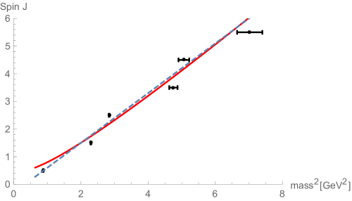
Figure 1: A plot of (4.4) compared with the experimental data. The dots with error bars represent the data listed in Table 7. The solid line is the plot of (4.4) with $\alpha^{\prime}\simeq 0.6\,{\rm GeV}^{-2}$ and $M_{0}^{\prime}\simeq 0.5\,{\rm GeV}$, while the dashed line is the linear trajectory (4.5) with $\alpha_{0}\simeq-0.3$ and $\alpha^{\prime}\simeq 0.9\,{\rm GeV}^{-2}$.

Due to the nonlinear term in (4.4), the trajectory in Figure 1 is curved toward the left and the value of mass squared for $J=1/2$ becomes significantly smaller compared to that of the nucleons (proton or neutron). This is, however, not a problem of the formula (4.4) as it is derived for the states with $J\geq 3/2$. Our expression for the nucleon mass is given in (4.1). Though we are not able to predict its value, this observation suggests that the difference between (4.1) and $M_{0}^{\prime}$

$$M_{{\mathcal{N}}=0}-M_{0}^{\prime}=M_{0}^{*}(q_{w}=N_{c},\ell=1)-M_{0}^{*}(q_{w}=N_{c}-1,\ell=0)\ ,$$ (4.7)

is positive, as expected.

We emphasize that the values (4.6) should not be considered to be an accurate estimate, because we have neglected all the $1/N_{c}$ and $1/\lambda$ corrections, as well as the possible contributions from the interaction term (3.50) for the massive fields. Nevertheless, let us make a few comments here on the value of $\alpha^{\prime}$. In [2, 3], the parameters $M_{\rm KK}$ and $\lambda$ were chosen to be

$$M_{\rm KK}\simeq 949\,{\rm MeV}\ ,~{}~{}\lambda\simeq 16.6\ ,$$ (4.8)

to fit the experimental values of the $\rho$-meson mass and the pion decay constant. If we use these values and the relation (2.4), we obtain $\alpha^{\prime}\simeq 0.452\,{\rm GeV}^{-2}$, which is a bit small compared with the value in (4.6). On the other hand, the value of $\alpha^{\prime}$ evaluated from the Regge slope of the $\rho$-meson trajectory is $\alpha^{\prime}|_{\rm exp}\simeq 0.88~{}{\rm GeV}^{-2}$. In [8], the $\rho$-meson Regge behavior is analyzed theoretically using the same holographic model of QCD as in the present paper. It was argued there that the $\rho$-meson trajectory has some nonlinear corrections similar to that in (4.4) and the value of $\alpha^{\prime}$ that fits well with the experimental data turned out to be around $1.1~{}{\rm GeV}^{-2}$. The value of $\alpha^{\prime}$ in (4.6) is close to neither of these values, though it is not too far from them. It is important to resolve this discrepancy by making more accurate estimate of $\alpha^{\prime}$.

Note that the slope $\alpha^{\prime}$ of the linear Regge trajectory (4.5) for the excited nucleons is very close to that of the $\rho$-mesons. This is one of the motivations for conjecturing that both of them are described by open strings with some particles attached on the end points as investigated in [25, 26]. Our description is similar to these models in that only one of $N_{c}$ strings attached on the baryon vertex gets excited while the rest remain in the ground state. This system may be approximated with a single open string by regarding the effect of the baryon vertex as a massive end point. However, a clear distinction from the models in [25, 26] is that the mass of the end point in the present model is of ${\mathcal{O}}(N_{c})$ and considered to be much heavier than the energy scale determined by the string tension. In fact, it is not difficult to verify that a rotating open string with a massive end point of mass $M_{0}$ has a classical energy $E$ that reduces in the heavy end point limit to

$$J=2\alpha^{\prime}(E-M_{0})^{2}\ ,$$ (4.9)

which agrees with (4.4) up to an additive constant $1/2$ and the contributions from the zero-point energy in $M_{0}^{\prime}$. We note that the difference between the mass formula (4.4) and (4.9) is due to quantum $1/N_{c}$ corrections.

4.2 More about excited baryon states

In this subsection, we show some examples of low-lying excited baryons that are obtained in a manner explained in the previous sections. For simplicity, we set $(n_{\rho},n_{z})=(0,0)$ and $n_{\beta}^{a}=0$. The states in the massless and massive sectors are denoted by $|\ell,q_{w}\rangle$ and $|n_{j}^{\Psi},n_{j}^{\overline{\Psi}},n_{k}^{\Phi}\rangle$, respectively, where only nonvanishing quantum numbers are indicated explicitly for notational simplicity.

We start from the sector ${\mathcal{N}}=1/2$. This sector is constructed only from the excitation of a single 8-4 string with $N_{84}^{(1)}=1/2$, because any 4-4 excited state has $N_{44}^{(k)}\geq 1$. The corresponding field $\Psi_{1}$ belongs to $(1,1/2)_{-}$ under $SU(2)_{L}\times SU(2)_{R}$ with the subscript denoting parity, and yields a harmonic oscillator with angular frequency given by $m_{1}=\sqrt{1/(2\alpha^{\prime})}$. The condition ${\mathcal{N}}_{84}=1/2$ is satisfied when $(n_{1}^{\Psi},n_{1}^{\overline{\Psi}})=(1,0)$ or $(0,1)$. The excited states $|n_{1}^{\Psi}=1\rangle$ and $|n_{1}^{\overline{\Psi}}=1\rangle$ have the same energy eigenvalue of $H_{m}$ with $SU(2)_{L}\times SU(2)_{R}$ spin given by $(1,1/2)_{-}$. We consider only the former, because this leads to $q_{w}=N_{c}-1$ so that (3.34) shows that the corresponding massless sector has less energy compared to that with $q_{w}=N_{c}+1$, which corresponds to $|n_{1}^{\overline{\Psi}}=1\rangle$. As $q_{w}$ is even, the massless sector is allowed to have $\ell=0,2,4,\cdots$. We first consider the case $\ell=0$, which yields the lightest state in the massless sector $\ket{\ell=0,q_{w}}$, which belongs to the trivial $SU(2)_{L}\times SU(2)_{I}$ representation and has even parity because $n_{z}=0$. Hence, the tensor product state of $\ket{\ell=0,q_{w}}$ with $|n_{1}^{\Psi}=1\rangle$ has $SU(2)_{L}\times SU(2)_{R}\times SU(2)_{I}$ spin given by

$$(1,1/2)^{1/2}_{-}\otimes(0,0)^{0}_{+}=(1,1/2)^{1/2}_{-}\ ,$$ (4.10)

where the superscripts represent the isospin. The tensor product state of $\ket{\ell=2,q_{w}}$ with $|n_{1}^{\Psi}=1\rangle$ decomposes under $SU(2)_{L}\times SU(2)_{R}\times SU(2)_{I}$ as

$$(1,1/2)^{1/2}_{-}\otimes(1,0)^{1}_{+}=\left[(2,1/2)\oplus(1,1/2)\oplus(0,1/2)\right]^{3/2}_{-}\oplus\left[(2,1/2)\oplus(1,1/2)\oplus(0,1/2)\right]^{1/2}_{-}\ .$$

It is straightforward to decompose all these states in terms of $SU(2)_{J}\subset SU(2)_{L}\times SU(2)_{R}$. The results are summarized in Table 8.

product states	$SU(2)_{L}\times SU(2)_{R}\times SU(2)_{I}$	$SU(2)_{J}\times SU(2)_{I}$
$|\ell=0,q_{w}=N_{c}-1\rangle\otimes|n_{1}^{\Psi}=1\rangle$	$(1,1/2)^{1/2}_{-}$	$(3/2)^{1/2}_{-}\oplus(1/2)^{1/2}_{-}$
$|\ell=2,q_{w}=N_{c}-1\rangle\otimes|n_{1}^{\Psi}=1\rangle$	$\left[(2,1/2)\oplus(1,1/2)\oplus(0,1/2)\right]^{3/2}_{-}$	$[(5/2)\oplus 2(3/2)\oplus 2(1/2)]^{3/2}_{-}$
	$\oplus\left[(2,1/2)\oplus(1,1/2)\oplus(0,1/2)\right]^{1/2}_{-}$	$\oplus[(5/2)\oplus 2(3/2)\oplus 2(1/2)]^{1/2}_{-}$

Table 8: Excited baryon states for ${\mathcal{N}}=1/2$.

Note that $(3/2)^{1/2}_{-}$ appearing in the first row is identified with N(1520) in the previous section.

We next turn to discussing the ${\mathcal{N}}=1$ states. This is possible only when $({\mathcal{N}}_{84},{\mathcal{N}}_{44})=(1,0)$ or $(0,1)$. The first condition is further divided into two cases: (i) $(n_{1}^{\Psi},n_{1}^{\overline{\Psi}})=(2,0),(1,1),(0,2)$ and (ii) $(n_{j}^{\Psi},n_{j}^{\overline{\Psi}})=(1,0),(0,1)$ for $j=2,3,4$. Note that the 8-4 massive states with $j=2,3,4$ are given by the three states with $N_{84}=1$ listed in Table 5. Again, we focus on the lightest states in each case, implying that we pick up only $(n_{1}^{\Psi},n_{1}^{\overline{\Psi}})=(2,0)$ and $(n_{j}^{\Psi},n_{j}^{\overline{\Psi}})=(1,0)$ with $j=2,3,4$. The second condition $({\mathcal{N}}_{84},{\mathcal{N}}_{44})=(0,1)$ is solved by $n_{k}^{\Phi}=1$ with $k=1,2,3,4$ with the rest of the excitation numbers set to zero. Note that the 4-4 string states labeled by $k=1,2,3,4$ are given by the excited states with $N_{44}=1$ shown in Table 6. As no excitation is made by any 8-4 string mode, this case gives $q_{w}=N_{c}$.

Let us now work out the baryon states for the above three cases. For the first case, the state in the massive sector is given by $|n_{1}^{\Psi}=2\rangle$, which transforms under $SU(2)_{L}\times SU(2)_{R}\times SU(2)_{I}$ as

$$\left[(1,1/2)_{-}^{1/2}\otimes(1,1/2)_{-}^{1/2}\right]_{\rm symmetrized}=\left[(0,1)^{1}\oplus(0,0)^{0}\oplus(2,1)^{1}\oplus(2,0)^{0}\oplus(1,1)^{0}\oplus(1,0)^{1}\right]_{+}\ .$$ (4.11)

The massless sector for this case is characterized by $q_{w}=N_{c}-2={\rm odd}$. We are thus allowed to set $\ell=1$ as the lightest state, whose $SU(2)_{L}\times SU(2)_{R}\times SU(2)_{I}$ spin is given by $(1/2,0)_{+}^{1/2}$. By taking the tensor product of this state $\ket{\ell=1,q_{w}=N_{c}-2}$ with $|n_{1}^{\Psi}=2\rangle$, we find the following baryon states:

$$[(1/2,0)\oplus(1/2,1)\oplus(3/2,0)\oplus(3/2,1)\oplus(5/2,1)]_{+}^{3/2}$$

$$\oplus[2(1/2,0)\oplus 2(1/2,1)\oplus 2(3/2,0)\oplus 2(3/2,1)\oplus(5/2,0)\oplus(5/2,1)]_{+}^{1/2}\ .$$ (4.12)

For the second case, we take the massive sector state to be $|n_{j}^{\Psi}=1\rangle$ with $j=2,3,4$. This corresponds to $q_{w}=N_{c}-1={\rm even}$. We can take $\ell=0,2,4\cdots$. The state $\ket{\ell=0,q_{w}}$ has a trivial spin so that the tensor product of this state with $|n_{j}^{\Psi}=1\rangle$ has the same spin as $|n_{j}^{\Psi}=1\rangle$. The massless sector with $\ell=2$ has $SU(2)_{L}\times SU(2)_{R}\times SU(2)_{I}$ spin given by $(1,0)^{1}$. The tensor product of this state with $|n_{j}^{\Psi}=1\rangle$ is easy to evaluate for each $j=2,3,4$.

Finally, the massive sector for the third case is characterized by the four states $|n_{k}^{\Phi}=1\rangle$ with $k=1,2,3,4$. As noted before, this corresponds to $q_{w}=N_{c}={\rm odd}$ so that odd $\ell$ is allowed. We pick up $\ell=1$, which is expected to give the lightest state among those with odd $\ell$, and take its tensor product with $|n^{\Phi}_{k}=1\rangle$. Note that any 4-4 string state has a vanishing isospin. The same computation is easy to perform for the next-lightest state with $\ell=3$.

All the results are summarized in Table 9.

product states	$SU(2)_{L}\times SU(2)_{R}\times SU(2)_{I}$
$|\ell=1,q_{w}=N_{c}-2\rangle\otimes|n_{1}^{\Psi}=2\rangle$	$[(1/2,0)\oplus(1/2,1)\oplus(3/2,0)\oplus(3/2,1)\oplus(5/2,1)]_{+}^{3/2}$
	$\oplus[2(1/2,0)\oplus 2(1/2,1)\oplus 2(3/2,0)\oplus 2(3/2,1)\oplus(5/2,0)\oplus(5/2,1)]_{+}^{1/2}$
$|\ell=0,q_{w}=N_{c}-1\rangle\otimes|n_{2}^{\Psi}=1\rangle$	$(1/2,0)^{1/2}_{+}$
$|\ell=0,q_{w}=N_{c}-1\rangle\otimes|n_{3}^{\Psi}=1\rangle$	$(1/2,1)_{+}^{1/2}$
$|\ell=0,q_{w}=N_{c}-1\rangle\otimes|n_{4}^{\Psi}=1\rangle$	$(3/2,1)_{+}^{1/2}$
$|\ell=2,q_{w}=N_{c}-1\rangle\otimes|n_{2}^{\Psi}=1\rangle$	$[(3/2,0)\oplus(1/2,0)]^{3/2}_{+}\oplus[(3/2,0)\oplus(1/2,0)]^{1/2}_{+}$
$|\ell=2,q_{w}=N_{c}-1\rangle\otimes|n_{3}^{\Psi}=1\rangle$	$[(3/2,1)\oplus(1/2,1)]^{3/2}_{+}\oplus[(3/2,1)\oplus(1/2,1)]^{1/2}_{+}$
$|\ell=2,q_{w}=N_{c}-1\rangle\otimes|n_{4}^{\Psi}=1\rangle$	$[(5/2,1)\oplus(3/2,1)\oplus(1/2,1)]^{3/2}_{+}\oplus[(5/2,1)\oplus(3/2,1)\oplus(1/2,1)]^{1/2}_{+}$
$|\ell=1,q_{w}=N_{c}\rangle\otimes|n_{1}^{\Phi}=1\rangle$	$(1/2,0)^{1/2}_{+}$
$|\ell=1,q_{w}=N_{c}\rangle\otimes|n_{2}^{\Phi}=1\rangle$	$(1/2,0)^{1/2}_{+}$
$|\ell=1,q_{w}=N_{c}\rangle\otimes|n_{3}^{\Phi}=1\rangle$	$\left[(1,1/2)\oplus(0,1/2)\right]^{1/2}_{-}$
$|\ell=1,q_{w}=N_{c}\rangle\otimes|n_{4}^{\Phi}=1\rangle$	$[(3/2,1)\oplus(1/2,1)]^{1/2}_{+}$
$|\ell=3,q_{w}=N_{c}\rangle\otimes|n_{1}^{\Phi}=1\rangle$	$(3/2,0)^{3/2}_{+}$
$|\ell=3,q_{w}=N_{c}\rangle\otimes|n_{2}^{\Phi}=1\rangle$	$(3/2,0)^{3/2}_{+}$
$|\ell=3,q_{w}=N_{c}\rangle\otimes|n_{3}^{\Phi}=1\rangle$	$\left[(2,1/2)\oplus(1,1/2)\right]^{3/2}_{-}$
$|\ell=3,q_{w}=N_{c}\rangle\otimes|n_{4}^{\Phi}=1\rangle$	$[(5/2,1)\oplus(3/2,1)\oplus(1/2,1)]^{3/2}_{+}$

Table 9: Excited baryon states for ${\mathcal{N}}=1$.

Decomposing these states in terms of $SU(2)_{J}\subset SU(2)_{L}\times SU(2)_{R}$ is straightforward.

Now we discuss possible identifications of the states listed in Tables 8 and 9 with the baryons found in experiments. Because we have not been able to derive the $\ell$ dependence in the baryon mass formula (3.33), we have to rely on some qualitative arguments. Our guiding principles are as follows. First, we expect that the states with the same $\ell$, $q_{w}$ and ${\mathcal{N}}$ are nearly degenerate. Second, for a given $(\ell,q_{w})$, the states with ${\mathcal{N}}=1$ are heavier than those with ${\mathcal{N}}=1/2$. Third, for a given ${\mathcal{N}}$, the mass is an increasing function of both $\ell$ and $q_{w}$ except for the state with $n_{1}^{\Psi}=2$ listed in the first row of Table 9, which is expected to be heavier than the others according to the baryon mass formula (3.33).

The predictions for the low-lying excited baryons with $I=1/2$ are summarized in Table 10, whose data are taken from Tables 8 and 9.

level	states	$SU(2)_{J}\times SU(2)_{I}$
${\mathcal{N}}=1/2$	$|\ell=0,q_{w}=N_{c}-1\rangle\otimes|n_{1}^{\Psi}=1\rangle$	$[{\color[rgb]{0,0,1}(3/2)}\oplus(1/2)]_{-}^{1/2}$
	$|\ell=2,q_{w}=N_{c}-1\rangle\otimes|n_{1}^{\Psi}=1\rangle$	$[(5/2)\oplus 2(3/2)\oplus 2(1/2)]_{-}^{1/2}$
${\mathcal{N}}=1$	$|\ell=0,q_{w}=N_{c}-1\rangle\otimes|n_{2,3,4}^{\Psi}=1\rangle$	$[{\color[rgb]{0,0,1}(5/2)}\oplus 2(3/2)\oplus 3(1/2)]_{+}^{1/2}$
	$|\ell=1,q_{w}=N_{c}\rangle\otimes|n_{1,2,3,4}^{\Phi}=1\rangle$	$[(5/2)\oplus 2(3/2)\oplus 4(1/2)]_{+}^{1/2}\oplus[(3/2)\oplus 2(1/2)]_{-}^{1/2}$
	$|\ell=2,q_{w}=N_{c}-1\rangle\otimes|n_{2,3,4}^{\Psi}=1\rangle$	$[(7/2)\oplus 3(5/2)\oplus 6(3/2)\oplus 5(1/2)]_{+}^{1/2}$

Table 10: Low-lying excited baryons with $I=1/2$. Here we have omitted the states with $n_{1}^{\Psi}=2$ in Table 9. The blue-colored states are identified with excited baryons lying on the nucleon Regge trajectory in section 4.1.

We will not attempt to relate the states with $J=1/2$ in this table to those in the baryon summary table [23], here, because these might be regarded as excited states with nonvanishing $n_{\rho}$, $n_{z}$ and $n_{\beta}$ without excitations in the massive sector. Note that the states with $(3/2)_{-}^{1/2}$ and $(5/2)_{+}^{1/2}$ in the first and third rows of Table 10 are identified with N(1520) and N(1680), respectively, in section 4.1. The $(5/2)_{-}^{1/2}$ state at ${\mathcal{N}}=1/2$ is expected to be the lightest state with this quantum number and hence it may be identified with N(1675), which is the lightest baryon with the same quantum number listed in the baryon summary table. Then, the $(3/2)_{-}^{1/2}$ states in the second row are expected to have mass nearly equal to N(1675). A natural candidate for one of them is N(1700).

As for the ${\mathcal{N}}=1$ states, we find that the $(3/2)_{+}^{1/2}$ states in the third row of Table 10 are expected to have mass nearly equal to N(1680). A natural candidate for one of them is N(1720). Since the fourth row has larger values of $\ell$ and $q_{w}$ compared with the third row, the $(5/2)_{+}^{1/2}$ state in the fourth row is expected to be heavier than N(1680) and N(1720). A natural candidate for it is N(1860), though this state has not been established in experiments. If this is the case, the $(3/2)_{\pm}^{1/2}$ states in the fourth row are expected to be nearly degenerate with N(1860). These states could be identified with N(1900) and N(1875). The baryon states in the fifth row contain a state with $(7/2)_{+}^{1/2}$. The only baryon with this quantum number listed in the baryon summary table is N(1990), though this is not considered to be established. Then, the $(5/2)_{+}^{1/2}$ and $(3/2)_{+}^{1/2}$ states in the fifth row of Table 10 could be identified with N(2000) and N(2040), respectively, which are again poorly established in experiments.

Unfortunately, the identification we have made is not a clear one-to-one correspondence. There is more than one candidate state in the model for many of the baryons listed in the baryon summary table. In particular, the degeneracy of the states in Table 10 does not match the experimental data perfectly. Furthermore, as mentioned in the footnotes, some of the baryons may be identified with the states that are not listed in Table 10. This lack of the one-to-one correspondence could in part be because all the excited baryons we consider are unstable resonances (for finite $N_{c}$), and many of them, in particular the heavier ones, are probably not easy to identify in experiments. Furthermore, some of the states in Tables 10 and 11 could be artifacts of the model. Although, as discussed in section 2, we have imposed invariance with respect to the $SO(5)$ symmetry and $\tau$-parity to get rid of artifacts, we are not able to show that this is sufficient to exclude all of them. It is expected that incorporation of full $1/\lambda$ corrections into the baryon mass formula makes the artifacts of the model infinitely heavy in the $M_{\rm KK}\rightarrow\infty$ ($\lambda\rightarrow 0$) limit with $\Lambda_{\rm QCD}$ kept fixed. However, the extrapolation to the small $\lambda$ regime is a notoriously difficult problem in the holographic description, because we have to deal with all the stringy corrections in a highly curved spacetime. A similar observation was also made in [4]. We leave as an open problem the study of a dictionary between the theoretical predictions and the experimental data in more detail.

We also examine the mass spectrum of $\Delta$ baryons with isospin $I=3/2$. The theoretical predictions for this case are summarized in Table 11, whose data is taken from Tables 8 and 9.

level	states	$SU(2)_{J}\times SU(2)_{I}$
${\mathcal{N}}=1/2$	$|\ell=2,q_{w}=N_{c}-1\rangle\otimes|n_{1}^{\Psi}=1\rangle$	$[(5/2)\oplus 2(3/2)\oplus 2(1/2)]_{-}^{3/2}$
${\mathcal{N}}=1$	$|\ell=2,q_{w}=N_{c}-1\rangle\otimes|n_{2,3,4}^{\Psi}=1\rangle$	$[(7/2)\oplus 3(5/2)\oplus 6(3/2)\oplus 5(1/2)]_{+}^{3/2}$

Table 11: Low-lying excited baryons with $I=3/2$. In this table, we have omitted the states with $n_{1}^{\Phi}=2$ and $\ell=3$ in Table 9.

It is natural to identify the $(5/2)_{-}^{3/2}$ and $(7/2)_{+}^{3/2}$ states in the first and second rows of Table 11 with the lightest $\Delta$ baryons having the same quantum numbers listed in the baryon summary table, which are $\Delta(1930)$ and $\Delta(1950)$, respectively. This suggests that the $(5/2)_{+}^{3/2}$ states in the second row of Table 9 are nearly degenerate with $\Delta(1950)$. A good candidate to be identified with one of these states is $\Delta(1905)$. However, this identification is problematic: although our formula (3.33) suggests that the ${\mathcal{N}}=1$ states are significantly heavier than the ${\mathcal{N}}=1/2$ states, $\Delta(1930)$ and $\Delta(1950)$ are nearly degenerate and $\Delta(1905)$ is even lighter than $\Delta(1930)$.

5 Conclusions

We have discussed stringy excited baryons using the holographic dual of QCD on the basis of an intersecting D4/D8-brane system. A key step to this end is to work on the whole system of a baryon vertex without describing it by a topological soliton on an effective 5 dimensional gauge theory. We formulated this system as a many-body quantum mechanics that is composed of the ADHM-type matrix model of Hashimoto-Iizuka-Yi [13] and an infinite number of open string massive modes. This is done by relying on an approximation that is valid in the large $N_{c}$ and $\lambda$ regime. The resultant quantum mechanics provides us with a powerful framework for making a systematic analysis of excited baryons including those with $I\neq J$ that are difficult to obtain in the soliton picture.

By construction, it would be too ambitious for the theoretical predictions from the present model to match the experimental data to good accuracy. Interestingly, we have seen that the present model reproduces a qualitative feature of the nucleon Regge trajectory. It has been argued that the stringy excited baryons to be identified with the excited nucleons are interpreted as a rotating open string with a massive end point. Such a picture of baryon Regge trajectories has been studied extensively in the literature. [25, 26] It is worth emphasizing that the massive end point in this model is due to a D4_BV, having a mass of ${\mathcal{O}}(N_{c})$. The Regge trajectory formula (4.4) that we proposed in this paper is not given by a simple, linear relation between the spin and the mass squared because of the heavy end point.

We conclude this paper by making some comments about future directions. First, it is important to improve the theoretical accuracy of the model by incorporating the interacting terms in $L_{\rm int}$ that have been neglected for technical difficulties. It would be almost impossible to fix the mass terms of the mass fields $\Psi_{j}$ and $\Phi_{k}$ precisely, because infinitely many higher-order terms could contribute to a single mass term, as discussed in section 3.7. Instead, what may be performed immediately is to take into account the effects of the mixing terms like $\Psi_{j}\Psi_{j}$ in the baryon mass formula. With these mixing terms, $q_{j}$ is not a conserved charge any more so that an exact diagonalization of $H_{m}$ in a manner consistent with the Gaussian constraint appears highly involved. It would be interesting to compute the perturbative effect of the mixing terms into the mass formula.

One of the unsatisfactory points is that the values of the parameters $\gamma$ and $v$ in the potential (3.5) are not determined from first principles. Though it is possible to adjust them to fit the results in the soliton picture as in [7], a derivation within our framework is desired to make sure that all the parameters can be fixed, in principle, without any ambiguities. Compared with the soliton picture, the origin of the potential (3.5) is expected to be due to the energy contribution from the $U(N_{f})$ gauge field on the flavor D8-branes in the presence of a baryon vertex. It would be interesting to examine this in more detail.

Finally, it would be of great interest to apply the results in this paper to a more complicated system made out of multiple baryon and anti-baryon vertices. A typical example is given by a stringy realization of tetraquarks. It would be nice to try to formulate a holographic model for tetraquarks following this paper and compare the theoretical predictions with experiments.

Appendix A $SO(4)\simeq SU(2)_{I}\times SU(2)_{J}$

The generators of the Lie algebra of $SO(4)\simeq(SU(2)_{I}\times SU(2)_{J})/{\mathbb{Z}}_{2}$ can be chosen as

$$i\Sigma^{1} = i\sigma_{2}\otimes\sigma_{1}=\left(\begin{array}[]{cc}&\sigma_{1}\\ -\sigma_{1}&\end{array}\right)\ ,$$ (A.3)

$$i\Sigma^{2} = -i\sigma_{2}\otimes\sigma_{3}=\left(\begin{array}[]{cc}&-\sigma_{3}\\ \sigma_{3}&\end{array}\right)\ ,$$ (A.6)

$$i\Sigma^{3} = i{\bf 1}_{2}\otimes\sigma_{2}=\left(\begin{array}[]{cc}i\sigma_{2}&\\ &i\sigma_{2}\end{array}\right)\ ,$$ (A.9)

$$i\widetilde{\Sigma}^{1} = -i\sigma_{1}\otimes\sigma_{2}=\left(\begin{array}[]{cc}&-i\sigma_{2}\\ -i\sigma_{2}&\end{array}\right)\ ,$$ (A.12)

$$i\widetilde{\Sigma}^{2} = -i\sigma_{2}\otimes{\bf 1}_{2}=\left(\begin{array}[]{cc}&-{\bf 1}_{2}\\ {\bf 1}_{2}&\end{array}\right)\ ,$$ (A.15)

$$i\widetilde{\Sigma}^{3} = i\sigma_{3}\otimes\sigma_{2}=\left(\begin{array}[]{cc}i\sigma_{2}&\\ &-i\sigma_{2}\end{array}\right)\ .$$ (A.18)

$\{\Sigma^{a}\}$ and $\{\widetilde{\Sigma}^{a}\}$ satisfy the same algebra as the Pauli matrices

$$\Sigma^{a}\Sigma^{b}=\delta^{ab}+i\epsilon^{abc}\Sigma^{c}\ ,~{}~{}~{}\widetilde{\Sigma}^{a}\widetilde{\Sigma}^{b}=\delta^{ab}+i\epsilon^{abc}\widetilde{\Sigma}^{c}\ ,$$ (A.19)

and they commute with each other

$$\Sigma^{a}\widetilde{\Sigma}^{b} = \widetilde{\Sigma}^{b}\Sigma^{a}\ .$$ (A.20)

$\{i\Sigma^{a}\}_{a=1,2,3}$ and $\{i\widetilde{\Sigma}^{a}\}_{a=1,2,3}$ are the generators of $SU(2)_{I}$ and $SU(2)_{J}$, respectively.

References

• [1] O. Aharony, S. S. Gubser, J. M. Maldacena, H. Ooguri and Y. Oz, “Large N field theories, string theory and gravity,” Phys. Rept.  323, 183 (2000) [hep-th/9905111].
• [2] T. Sakai and S. Sugimoto, “Low energy hadron physics in holographic QCD,” Prog. Theor. Phys.  113, 843 (2005) [hep-th/0412141].
• [3] T. Sakai and S. Sugimoto, “More on a holographic dual of QCD,” Prog. Theor. Phys.  114, 1083 (2005) [hep-th/0507073].
• [4] T. Imoto, T. Sakai and S. Sugimoto, “Mesons as Open Strings in a Holographic Dual of QCD,” Prog. Theor. Phys.  124, 263 (2010) [arXiv:1005.0655 [hep-th]].
• [5] T. H. R. Skyrme, “A Nonlinear field theory,” Proc. Roy. Soc. Lond. A 260, 127 (1961).
• [6] G. S. Adkins, C. R. Nappi and E. Witten, “Static Properties of Nucleons in the Skyrme Model,” Nucl. Phys. B 228, 552 (1983).
• [7] H. Hata, T. Sakai, S. Sugimoto and S. Yamato, “Baryons from instantons in holographic QCD,” Prog. Theor. Phys.  117, 1157 (2007) [hep-th/0701280 [HEP-TH]].
• [8] K. Hashimoto, T. Sakai and S. Sugimoto, “Holographic Baryons: Static Properties and Form Factors from Gauge/String Duality,” Prog. Theor. Phys.  120 (2008) 1093 [arXiv:0806.3122 [hep-th]].
• [9] D. K. Hong, M. Rho, H. U. Yee and P. Yi, “Chiral Dynamics of Baryons from String Theory,” Phys. Rev. D 76 (2007) 061901 [hep-th/0701276 [HEP-TH]], D. K. Hong, M. Rho, H. U. Yee and P. Yi, “Dynamics of baryons from string theory and vector dominance,” JHEP 0709 (2007) 063 [arXiv:0705.2632 [hep-th]].
• [10] H. Hata, M. Murata and S. Yamato, “Chiral currents and static properties of nucleons in holographic QCD,” Phys. Rev. D 78 (2008) 086006 [arXiv:0803.0180 [hep-th]].
• [11] K. Y. Kim and I. Zahed, “Electromagnetic Baryon Form Factors from Holographic QCD,” JHEP 0809 (2008) 007 [arXiv:0807.0033 [hep-th]].
• [12] K. Hashimoto, Y. Matsuo and T. Morita, “Nuclear states and spectra in holographic QCD,” JHEP 1912, 001 (2019) [arXiv:1902.07444 [hep-th]].
• [13] K. Hashimoto, N. Iizuka and P. Yi, “A Matrix Model for Baryons and Nuclear Forces,” JHEP 1010, 003 (2010) [arXiv:1003.4988 [hep-th]].
• [14] E. Witten, “Baryons and branes in anti-de Sitter space,” JHEP 9807, 006 (1998) [hep-th/9805112].
• [15] D. J. Gross and H. Ooguri, “Aspects of large N gauge theory dynamics as seen by string theory,” Phys. Rev. D 58 (1998) 106002 [hep-th/9805129].
• [16] E. Witten, “Small instantons in string theory,” Nucl. Phys. B 460, 541 (1996) [hep-th/9511030].
• [17] M. R. Douglas, “Branes within branes,” NATO Sci. Ser. C 520, 267 (1999) [hep-th/9512077].
• [18] M. F. Atiyah, N. J. Hitchin, V. G. Drinfeld and Y. I. Manin, “Construction of Instantons,” Phys. Lett. A 65 (1978) 185.
• [19] E. Witten, “Anti-de Sitter space, thermal phase transition, and confinement in gauge theories,” Adv. Theor. Math. Phys.  2, 505 (1998) doi:10.4310/ATMP.1998.v2.n3.a3 [hep-th/9803131].
• [20] T. Imoto, T. Sakai and S. Sugimoto, “O(N(c)) and USp(N(c)) QCD from String Theory,” Prog. Theor. Phys.  122 (2010) 1433 [arXiv:0907.2968 [hep-th]].
• [21] R. C. Brower, S. D. Mathur and C. I. Tan, “Glueball spectrum for QCD from AdS supergravity duality,” Nucl. Phys. B 587, 249 (2000) [hep-th/0003115].
• [22] K. Hashimoto and N. Iizuka, “Nucleon Statistics in Holographic QCD : Aharonov-Bohm Effect in a Matrix Model,” Phys. Rev. D 82 (2010) 105023 [arXiv:1006.3612 [hep-th]].
• [23] M. Tanabashi et al. [Particle Data Group], “Review of Particle Physics,” Phys. Rev. D 98, no. 3, 030001 (2018).
• [24] S. S. Afonin, “Parity Doubling in Particle Physics,” Int. J. Mod. Phys. A 22 (2007) 4537 [arXiv:0704.1639 [hep-ph]].
• [25] G. S. Sharov, “String Models, Stability and Regge Trajectories for Hadron States,” arXiv:1305.3985 [hep-ph].
• [26] J. Sonnenschein and D. Weissman, “A rotating string model versus baryon spectra,” JHEP 1502 (2015) 147 [arXiv:1408.0763 [hep-ph]], J. Sonnenschein, “Holography Inspired Stringy Hadrons,” Prog. Part. Nucl. Phys.  92, 1 (2017) [arXiv:1602.00704 [hep-th]], J. Sonnenschein and D. Weissman, “Quantizing the rotating string with massive endpoints,” JHEP 1806, 148 (2018) [arXiv:1801.00798 [hep-th]].
• [27] G. S. Sharov, “Instability of classic rotational motion for three string baryon model,” hep-ph/0001154, G. S. Sharov, “Instability of the Y string baryon model within classical dynamics,” Phys. Atom. Nucl.  65 (2002) 906 [Yad. Fiz.  65 (2002) 938]. G. ’t Hooft, “Minimal strings for baryons,” hep-th/0408148,
• [28] E. Santopinto, “An Interacting quark-diquark model of baryons,” Phys. Rev. C 72 (2005) 022201 [hep-ph/0412319], C. L. Gutierrez and M. De Sanctis, “A relativistic quark-diquark model for the nucleon,” Pramana 72 (2009) 451, J. Ferretti, A. Vassallo and E. Santopinto, “Relativistic quark-diquark model of baryons,” Phys. Rev. C 83 (2011) 065204, C. Gutierrez and M. De Sanctis, “A study of a relativistic quark-diquark model for the nucleon,” Eur. Phys. J. A 50 (2014) no.11, 169.