On the roots of the Poupard
and Kreweras Polynomials
Abstract.
The Poupard polynomials are polynomials in one variable with integer coefficients, with some close relationship to Bernoulli and tangent numbers. They also have a combinatorial interpretation. We prove that every Poupard polynomial has all its roots on the unit circle. We also obtain the same property for another sequence of polynomials introduced by Kreweras and related to Genocchi numbers. This is obtained through a general statement about some linear operators acting on palindromic polynomials.
1. Introduction
Let us consider the sequence of polynomials in one variable characterized by the equation
| (1.1) |
with the initial condition . When described in this way, their existence is not completely obvious, because the right hand side must have a double root at for the recurrence to make sense. The first few terms are given by
The polynomial has degree and palindromic coefficients.
The coefficients of these polynomials form the Poupard triangle (A8301), first considered in 1989 by Christiane Poupard in the article [7] and proved there to enumerate some kind of labelled binary trees. It follows from this combinatorial interpretation that all coefficients of are nonnegative integers. For further combinatorial information on these polynomials and their relatives, see [1, 2].
The constant terms of these polynomials form the sequence of reduced tangent numbers (A2105), that can be defined for by the formula
| (1.2) |
where are the classical Bernoulli numbers, and starts by
One can deduce from (1.1) that , so the reduced tangent numbers also describe the values of the polynomials at .
Our first result is the following unexpected property, that was the experimental starting point of this article.
Theorem 1.1.
For , all roots of the polynomial are on the unit circle.
This is proved in section 2 in a much more general context, by showing that, for any positive integer , a linear operator maps palindromic polynomials with nonnegative coefficients to palindromic polynomials with nonnegative coefficients and all roots on the unit circle.
As another interesting application, one can consider the sequence of polynomials characterized by
| (1.3) |
with initial condition . The first few terms are
The polynomial has degree and palindromic coefficients.
Theorem 1.2.
For , all roots of the polynomial are on the unit circle.
Because the polynomials have odd degree, they are all divisible by . One can also show by induction that the polynomial is divisible by . The quotient polynomials have appeared in an article of Kreweras [3] dealing with refined enumeration of some sets of permutations. Their constant terms are the Genocchi numbers (A1469), given by the formula
| (1.4) |
where are again the Bernoulli numbers.
Both theorems above are proved in section 2 using a familly of operators acting on palindromic polynomials. Section 3 describes explicit simple eigenvectors of the operator . In section 4, some evidence is given for the general asymptotic behaviour of the iteration of the operators for . The last section contains various statements and conjectures on values of the operators on specific palindromic polynomials.
2. Operators and roots on the unit circle
Let us consider a polynomial with rational coefficients. Let us say that the polynomial is palindromic of index if for all . Note that the index can also be described as the sum of the degree and the valuation. For example, the index of the polynomial is . For any , let be the vector space spanned by palindromic polynomials of index .
For every nonnegative integer , let us introduce a linear operator from to . This operator is characterized by the following formula:
| (2.1) |
The definition requires that the right hand side is divisible by . By linearity of (2.1), it is enough to check this property for the basis elements with , where one finds
| (2.2) |
which is a polynomial with nonnegative integer coefficients. Note that when , one can divide (2.2) by .
The definition of and formula (2.2) imply immediately the following lemma.
Lemma 2.1.
Let be a non-zero palindromic polynomial of index with nonnegative integer coefficients. If , assume moreover that . Then is a non-zero palindromic polynomial of index with positive integer coefficients.
Let us record the following useful statement as a lemma.
Lemma 2.2.
When iterating times on an palindromic polynomial of odd index with integer coefficients, the integer divides .
Proof.
If the index of a palindromic polynomial is odd, then it is divisible by . When has integer coefficients, formula (2.1) then implies that has one further factor . The lemma follows by induction. ∎
Recall that a palindromic polynomial is called unimodal if the sequence of coefficients is increasing up to the middle coefficient(s), then decreasing. A polynomial is called concave if the piecewise linear function that maps to is a concave function. A concave polynomial is called strictly concave if every point is moreover an extremal point in the graph of this piecewise linear function.
Lemma 2.3.
Let be a non-zero palindromic polynomial of index with nonnegative integer coefficients. If , assume moreover that . Then is unimodal and concave. If has no zero coefficient, then is strictly concave.
Proof.
By (2.2), the polynomial is a nonnegative linear combination of unimodal and concave polynomials, hence itself unimodal and concave. Each term in (2.2) gives two extremal points, or just one extremal point when . When has no zero coefficient, this implies that there is an extremal point above every integer between and . ∎
Let us now recall a beautiful criterion obtained by Lakatos and Losonczi in [4].
Lemma 2.4.
Let be a palindromic polynomial of index . If
| (2.3) |
then all roots of are on the unit circle.
From this criterion, one deduces another one.
Theorem 2.5.
Let be a palindromic polynomial of index . If
| (2.4) |
with the convention that , then all roots of are on the unit circle.
Proof.
Let . Then , where
Note that is also palindromic of index .
Since is palindromic, and
one can therefore apply 2.4 to and conclude that has all its roots on the unit circle. This implies the same property for . ∎
Theorem 2.6.
Let be a non-zero palindromic polynomial of index with nonnegative integer coefficients. If , assume moreover that . Then is a non-zero palindromic polynomial of index with nonnegative integer coefficients and all roots of are on the unit circle.
Proof.
Let us now apply 2.6 to the proofs of 1.1 and 1.2. The defining recurrence (1.1) for the polynomials can be written as with the initial condition . The property follows by induction. The same proof works for with the initial polynomial .
Let us now state two useful lemmas.
Lemma 2.7.
For all , the polynomial is in the kernel of .
Proof.
This is a direct consequence of (2.2). ∎
Lemma 2.8.
Let be an integer. Then
| (2.5) |
Proof.
From the definition of by (2.2), and by the previous lemma, this is equal to
Developing, one find that the coefficient of is the cardinality of
But this is the same as the set
whose cardinality is . ∎
3. Sinus polynomials as eigenvectors
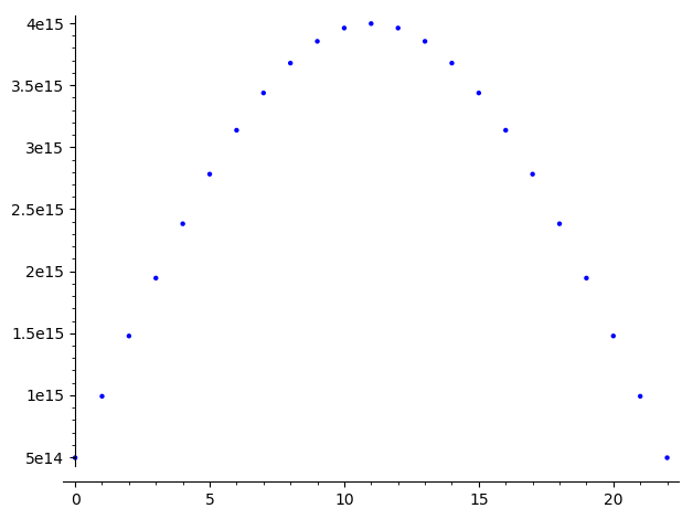
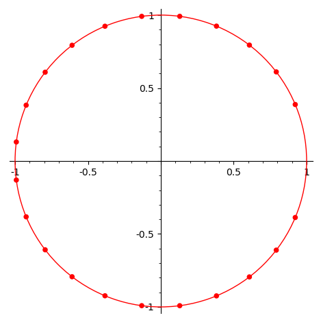
As can be seen in the right picture of fig. 1, the roots of the Poupard polynomials are very close to some of the roots of , with two missing roots on the right. Moreover the plot of the coefficients of seem to approximate a concave continuous function, as in the left picture of fig. 1.
One expects that, up to a global multiplicative factor, the polynomials obtained when iterating times the operator (for some fixed ) are always becoming, when is large, very close to the polynomials described in this section. Some kind of justification will be given in the next section.
Let us consider the polynomial defined for and odd by
| (3.1) |
whose roots are the roots of except and its conjugate.
Let us first give an alternative expression for .
Lemma 3.1.
The polynomial has an explicit expression
| (3.2) |
Proof.
The proof is a simple computation, expanding both sides as polynomials in and , also using that is odd. ∎
This implies that the plot of the coefficients of looks very much like a sinus curve, like the left image in fig. 1.
Proposition 3.2.
For every and odd , the polynomial is an eigenvector of the operator acting on , for the eigenvalue .
Proof.
Note that the eigenvalue is also the value .
In general, the Galois conjugates of the polynomial are not providing a complete set of eigenvectors for the operator acting on . The other eigenvectors are for odd divisors of , and their Galois conjugates.
The familly of operators acting on the spaces of palindromic polynomials looks very much like discrete versions of the Laplacian operator acting on the space of functions on the real interval such that for all and .
4. Asymptotic behaviour from recurrence
Our next point is to justify in a heuristic way that iterating an operator for some produces a sequence of polynomials that gets closer and closer to the sinus polynomials . We have not tried to make these computations rigourous.
Let us consider a familly of polynomials of index defined by iterating , starting from an arbitrary palindromic polynomial with nonnegative coefficients and index . In all this section, the index belongs to an arithmetic progression of step starting at . Let us denote
| (4.1) |
We will assume the following asymptotic ansatz for the constant terms:
| (4.2) |
for some constants , with positive. This ansatz is motivated by the known case of the tangent numbers, where , and . This ansatz implies that
| (4.3) |
We will also assume that there exists a smooth function which is a probability distribution function on the real interval vanishing at and , with on this interval and such that
| (4.4) |
is a good asymptotic approximation when is large, for some sequence to be determined.
Taking the sum of (4.4) over ranging from to and using the hypothesis on , one gets
Assuming that is negligible compared to , one obtains that a correct choice for is
From (2.1), one deduces that the action of at the level of coefficients is given by
| (4.5) |
except for and .
Using now the growth ansatz, one can get rid of in the rightmost term and obtain
| (4.7) |
The left hand side is an approximation of the second derivative of , so that one obtains
| (4.8) |
If , one therefore reaches the following differential equation
| (4.9) |
where . Because vanishes at , it must be a multiple of . Because vanishes at and is positive on the interval , necessarily and therefore . Because is a probability distribution, one must have .
One can therefore conclude that, under several plausible but unproven assumptions, the asymptotic shape of the coefficients of the polynomials is approximating that of the polynomials .
5. Various remarks
5.1. Action of the operator .
Applying the operator decreases the index by , so that iterating this operator on any initial polynomial of index always vanishes after a finite number of steps. Let be the last non-identically zero iterate of acting on . Let us denote by the linear map that maps to the constant term of .
For example, here is a sequence of iterates of :
In this case, .
Let us present some special cases of initial choices where the value of is interesting.
For , consider the polynomial
| (5.1) |
recording this sequence of final values. By antisymmetry of the argument of , the polynomial vanishes at . Let be the quotient , which is clearly a palindromic polynomial.
Proposition 5.1.
For every , the polynomial is the Poupard polynomial .
Proof.
For , one can check that . Assume . For , the coefficient of in can be written as
| (5.2) |
Let us now compute for . Starting from the left hand side of (5.2), this is given by
Using now the equation (2.2) for and the definition of as the final value for the iteration of , this becomes
in which one can recognize using the right hand side of (5.2).
Moreover, because is in the kernel of by 2.7.
Let us now check that . First, by (5.2), the left hand side is the image by of , given by 2.8. The right hand side is the image by of
| (5.3) |
which is the exact same expression.
All these properties of the coefficients imply exactly that the polynomial is the image of by , acting on the variable . ∎
For , consider the polynomial
| (5.4) |
recording this sequence of final values. By antisymmetry of the argument of , the polynomial vanishes at . Let be the quotient , which is clearly a palindromic polynomial of odd index.
Proposition 5.2.
For every , the polynomial is the Kreweras polynomial .
Proof.
The proof is very similar to the previous one. One first check that is . Then one checks by looking at coefficients that is . ∎
Let us now describe some similar conjectural properties. For the starting sequence , one gets the following values of :
which seem to be the Euler numbers A364. Similarly, for the starting sequence , one gets
This seems to be the closely related sequence A9843.
As a final conjectural remark, let us consider the following extension of the two previous cases.
Conjecture 5.3.
For every , the number is divisible by .
This property is clear if is odd by 2.2, but not at all if is even.
Assuming this conjecture, one can define, for every integer , the square matrix whose coefficient , for and , is .
Conjecture 5.4.
For all , the determinant of the matrix is given by the formula
| (5.5) |
where
For example, is equal to
| (5.6) |
whose determinant is indeed .
This matrix contains entries with large prime factors, for example , but the determinant has only small prime factors.
5.2. Action of the operator
Applying the operator does not change the index, so iterating this operator on any initial choice gives an infinite sequence of palindromic polynomials of the same index.
For example, starting with gives a sequence of polynomials
whose constant terms and middle coefficients are given by A7070 and by A6012. Indeed, the action of on reciprocal polynomials of index is given in the basis by the matrix
so that both sequences satisfy the recurrence with appropriate initial conditions.
5.3. Action of the operator .
Applying the operator increases the index by , so iterating this operator gives an infinite sequence of polynomials for every initial choice. In each such sequence, the sequence of constant terms is, up to a shift of indices by one, the same as the sequence of values at . Some examples were presented in the introduction, related to reduced tangent numbers and Genocchi numbers. Let us record one more familly of examples.
Using the polynomials for as starting points, one gets a table of constant terms:
Here is the row index and in each row the term of index is the constant term divided by . This table seems to be essentially the Salié triangle A65547.
References
- [1] D. Foata and G.-N. Han. Finite difference calculus for alternating permutations. J. Difference Equ. Appl., 19(12):1952–1966, 2013.
- [2] D. Foata and G.-N. Han. Tree calculus for bivariate difference equations. J. Difference Equ. Appl., 20(11):1453–1488, 2014.
- [3] G. Kreweras. Sur les permutations comptées par les nombres de Genocchi de 1-ière et 2-ième espèce. European J. Combin., 18(1):49–58, 1997.
- [4] P. Lakatos and L. Losonczi. Self-inversive polynomials whose zeros are on the unit circle. Publ. Math. Debrecen, 65(3-4):409–420, 2004.
- [5] M. N. Lalín and C. J. Smyth. Unimodularity of zeros of self-inversive polynomials. Acta Math. Hungar., 138(1-2):85–101, 2013.
- [6] M. N. Lalín and C. J. Smyth. Addendum to: Unimodularity of zeros of self-inversive polynomials [ 3015964]. Acta Math. Hungar., 147(1):255–257, 2015.
- [7] C. Poupard. Deux propriétés des arbres binaires ordonnés stricts. European J. Combin., 10(4):369–374, 1989.