Hedging problems for Asian options with transactions costs

Abstract

In this paper, we consider the problem of hedging Asian options in financial markets with transaction costs. For this we use the asymptotic hedging approach. The main task of asymptotic hedging in financial markets with transaction costs is to prove the probability convergence of the terminal value of the investment portfolio to the payment function when the number of portfolio revisions tends to be $n$ to infinity. In practice, this means that the investor, using such a strategy, is able to compensate payments for all financial transactions, even if their number increases unlimitedly.

1 Introduction

For a trader or an investor the main task is not only the saving but also the multiplication of its capital. Many risks can be avoided with the help of one popular and very effective technique – hedging. The option is hedged to protect its value from the risk of price movement of the underlying asset in an unfavorable direction. To solve the hedging problem stochastic calculus methods are used which became a powerful tool used in practice in the financial world. Stochastic calculus is a well-developed branch of modern mathematics with a “correct” approach to analyzing complex phenomena occurring on world stock markets.

In the modern theory and practice of options the paper written by Black and Scholes shishkova_Bl_Sch has an important role. In this work the authors used economic knowledge in combination with PDE arguments which are similar to deriving the heat equation from the first physical principles.

In our paper we use a probabilistic approach and our main tool is representation theorem for the Wiener process. This theorem was formulated by J.M.C. Clark in shishkova_clark also it can be obtained from the representation theorem stated in the paper shishkova_Ito by K. Ito.

It should be noted that the task of options pricing and the construction of a hedging strategy is well studied for American and European options, for such derivatives there is a so-called delta strategy. But this technique is not enough developed for Asian options. Exotic options became more in demand in the late 1980s and early 1990s and their trade became more active in the over-the-counter market. Soon in the commodity and currency markets, Asian options were becoming popular.

Mathematically, the value of an Asian option is reduced to calculating the conditional mathematical expectation of a payment function. Many authors have studieded in their work the Asian pricing problem. H. Geman and M. Yor (1993) were among the first to consider derivatives are based on the average prices of underlying assets Geman_1993 . Using the Bessel processes authors found the value of the Asian option. Moreover, applying simple probabilistic methods they obtained the following results about these options: calculated moments of all orders of the arithmetic average of the geometric Brownian motion; obtained simple, closed form expression of the Asian option price when the option is “in the money”. The exact pricing of fixed-strike Asian options is a difficult task, since the distribution of the average arithmetic of asset prices is unknown when its prices are distributed lognormally.

L. C. G. Rogers and Z. Shi (1995) in their work Rog_Shi_1995 to compute the price of an Asian option used two different ways. Firstly, exploiting a scaling property, they reduced the problem to the problem of solving a parabolic PDE in two variables. Secondly, authors provided a lower bound which is so accurate that it is essentially the true price. J. Vecer (2001) observed that the Asian option is a special case of the option on a traded account and extended work Shr_Vec_2000 to the arithmetic average Asian option Vec_2001 . Using probabilistic techniques he established that the price of the Asian option is characterized by a simple one-dimensional partial differential equation which could be applied to both continuous and discreteaverage Asian option. J.Vecer and M.Xu (2004) studied pricing Asian options in a semimartingale model Vec_Xu_2004 . They showed that the inherently path dependent problem of pricing Asian options can be transformed into a problem without path dependency in the payoff function. Authors also showed that the price satisfies a simpler integro-differential equation in the case the stock price is driven by a process with independent increments, Levy process being a special case. Pricing Asian options under Levy processes also considered in Shir_2008 ; Fusai_2008 ; Albrec_2004 .

When explicit valuation formulas are not available, sharp lower and upper bounds intervals for option prices can be useful in improving the quality of the approximations adopted: some results in this direction are provided in the papers Simon_2000 ; Vanm_2006 ; Zeng_2016 . In Niel_2003 authors considered geometric average Asian option and showed that the lower and upper bounds can be expressed as a portfolio of delayed payment European call options. Pricing Asian options with stochastic volatility considered in Fouq_2003 ; Huba_2016 ; Shi_2014 .

A large number of works are connected with the numerical approach. Kemna and Vorst were among the first who solved the task Kemna_1990 . In their work the pricing strategy includes Monte Carlo simulation with elements of dispersion reduction and improves the pricing method. Furthermore, the authors showed that the price of an option with an average value will always be lower than of a standard European option. Carverhill and Clewlow Carv_1990 used a fast Fourier transform to calculate the density of the sum of random variables, as convolution of individual densities. Then the payoff function is numerically integrated against the density. In this direction other authors continued to work, applying to the calculations improved methods of numerical simulation Lap_Tem_2001 ; Fu_Mad_1999 ; Segh_Lid_2008 . Unfortunately, these methods do not provide information on the hedging portfolio.

In the articles above, the authors focus on calculating the value of the option, but do not consider in detail the hedging problem, use only general existence theorems. In works Albr_2003 ; Jac_1996 authors consider the problem of hedging with the payoff

$$f=\left(\frac{S_{t_{1}}+...+S_{t_{n}}}{n}-K\right)_{+}$$

and use the moment recurrence technique, i.e. get recurrence equations. We can not use this technique, as we are considering the following payoff

$$f_{1}=\left(\int\limits_{0}^{1}S_{u}du-K\right)_{+}.$$

General equations for the hedging strategy based on the martingal representation

$$M_{t}={\bf E}(f|{\cal F}_{t})=M_{0}+\int\limits_{0}^{t}\alpha_{s}dW_{s},$$

where

$$\alpha_{s}=\langle M,W\rangle_{s}.$$

This theory is well developed only for options whose payoffs depend only on the price at the last moment in time $f=f(S_{T})$. And further, to compute a strategy, it is necessary to study only one random variable $S_{T}$, which is a geometric Brownian motion, i.e. density is known. In the case of Asian options, the payoff is a functional of the whole path and it is required to study the density of the integrals $\int\limits_{0}^{t}S_{u}du$ in order to calculate $\langle M,W\rangle_{s}$, that is, it is necessary to average over an infinite-dimensional distribution.

Yor and Dufrance Geman_1993 ; Dufr_2005 obtained the pricing in the explicit form, but they studied not the density, they considered the functional $f$, and for it they got a representation in the form of infinite series on a special orthogonal basis, which is not possible to study analiticaly the regularity properties. There is another method to study this properties of the density one can use the Brownian bridge, which proposed by Kabanov Yu.M. and Pergamenshchikov S.M. (2016) Kab_2016 . Using this method we construct the hedging strategy. This is made in shishkova_Shi_02_2018 .

It is worth noting that the option pricing model in work shishkova_Bl_Sch has an ideal character, i.e. it is assumed that it is friction-free market without costs. This theory is no longer true when we need to take into account transaction costs $\kappa_{n}J_{n}=\kappa_{0}n^{-\alpha}J_{n}$ because there is no unimprovable hedge. Therefore option pricing and replication with nonzero trading costs are different from that in the Black-Scholes setting.

Models with proportional transaction costs were considered as early as the 1970s. Magill and Constantinides shishkova_Mag_Const suggested in 1976 the consumption-investment model which is generalization of the Merton model of 1973 shishkova_Merton . However, the article written by H. Leland shishkova_Leland in 1985 became more important for practical application. Leland’s strategy provides an easy way to effectively eliminate the risks associated with transaction costs. This method is based on the idea that transaction costs can be offset by increasing the volatility parameter in the Black-Scholes strategy, that is the delta strategy obtained from a changed Black-Scholes equation with an appropriate modified volatility ensures an approximately complete replication as expected. The major goal in Leland’s algorithm is to explore the asymptotic behavior of the hedging error (difference between the terminal value of portfolio and the payoff function) as the number of transaction goes to infinity.

Leland suggested that if transaction costs are fixed, i.e. $\alpha=0$ then the value of the portfolio converges in probability to the payoff function as $n\rightarrow\infty$. He also suggested that this result will be true in the case of $\alpha=1/2$. Later this fact has proved by K. Lott in his thesis shishkova_Lott . Later Yu. Kabanov and M. Safarian shishkova_Kab_Saf extended Lott’s work to any $\alpha\in(0,1/2]$. Also they considered the case when $\alpha=0$, i.e. constant transaction cost. The authors proved that the hedging error admits a non-zero limit. The obtained result was used by H.Ahn end others shishkova_Ahn for the hedging problem with transaction costs in general diffusion models.

There are a lot of studies using Leland’s algorithm and extend it to various setting. For example, S. Pergamenshchikov in shishkova_perg studied the convergence rate of approximation in the case of constant costs. He obtained technically difficult result since used nontrivial procedure. This result is important because it not only provides asymptotic information about the hedging error but also gives a reasonable way to solve the hedging problem, namely, the investor can get a portfolio whose final value exceeds the desired profit by choosing the appropriate value of the modified volatility.

The important result had been obtained by E. Lepinette shishkova_Lepin1 in the case of time-depending volatility models. He used a non-uniform interval splitting. Moreover, to obtain the asymptotically complet replication he modified the strategy, which is called Lepinette’s strategy, and proved that for $\alpha>0$ the portfolio value of this strategy converges in probability to the payoff and if $\alpha=0$ then the portfolio value of strategy converges in probability to the payoff plus two positive functions depending on payoff. To improve a rate of convergence E. Lepinette in shishkova_Lepin2 also used a non-uniform interval splitting and proved that for strategy suggested in shishkova_Lepin1 with $\alpha=0$ the approximation error multiplied by $n^{\beta}$ weakly converges to a centered mixed Gaussian variable as $n\rightarrow\infty$.

Another way to enlarge application of Leland’s strategy is to consider the hedging problem with transaction costs in the models where the value of volatility depends on time and on the price of the stock, so-called the local volatility models. E.Lepinette and T.Tran shishkova_Lep_Tran extended results obtained in shishkova_Lepin2 to this models. The proof of the result is really complicated, since the existence of a solution of a non-uniform parabolic Cauchy problem is nontrivial, if we adjust the volatility as well as in work shishkova_Lepin1 .

To extend the Leland’s approach many others authors considered different situations including more general contingent claims, more general price processes and etc. see shishkova_Ngu ; shishkova_Den_Kab . Thus Leland’s strategy has great importance in option pricing and the hedging problem due to it is easily implemented in practice.

Our goal is to extend this hedging methods for the hedging problem for the financial markets with transaction costs. To this end we use the approximative hedging approach proposed Leland, Kabanov, Safarian, Pergamenshchikov, Lepinette shishkova_Leland ; shishkova_Kab_Saf ; shishkova_perg ; shishkova_Lepin1 . Note that is all this paper the hedging strategy is based on the delta-strategy. But for Asian option one need to change basic strategy, i.e. to pass frpm delta-strategy to Asian hedging strategy constructed in shishkova_Shi_02_2018 .

In this paper we study assymptotic property for the portfolio value with transaction cost in the Black-Scholes model with risky asset without drift and risk-free asset with interest rate $r=0$. We use the modification of Leland’s strategy. Main result of our study are obtined sufficient conditions, which provide assymptotic hedging.

2 Market model

2.1 Main condition

We consider the continuous time classical Black-Scholes model on financial market with risk- free asset (bond) and risky asset (stock). For simplicity we suppose that the risk-free rate $r=0$, i.e. the bond price is constant over time $B_{t}=1$ throughout this article. Let $(\Omega,{\cal F}_{1},({\cal F}_{t})_{0\leq t\leq 1},{\bf P})$ be the standard filtered probability space with ${\cal F}_{t}=\sigma(W_{s},0\leq s\leq t)$ and $W$ is a Wiener process. The asset price process $S_{t}$ given by

$$dS_{t}=\sigma S_{t}dW_{t},\;\;\;0\leq t\leq 1$$ (1)

and admit the following explicit form

$$S_{t}=S_{0}e^{\sigma W_{t}-\sigma^{2}t/2}.$$

Remark that $S_{t}$ is a martingale under measure ${\bf P}$. The model is considered on the interval $[0,1]$ where 1 is a maturity of the Asian option with payoff function

$$f_{1}=\left(\int\limits_{0}^{1}S_{u}du-K\right)_{+}.$$

2.2 Hedging problem

Definition 1

The financial strategy $(\Pi_{t})_{0\leq t\leq 1}=(\beta_{t},\gamma_{t})_{0\leq t\leq 1}$ is called an admissible self-financing strategy if it is ${\cal F}_{t}$-adapted, integrable with

$$\int\limits_{0}^{t}(|\beta_{t}|+\gamma_{t}^{2})dt<\infty$$

and the portfolio value is

$$V_{t}=\beta_{t}+\gamma_{t}S_{t}=V_{0}+\int\limits_{0}^{t}\gamma_{u}dS_{u}.$$

Here $V_{0}$ is an initial capital, $\beta_{t}$ and $\gamma_{t}$ are quantity of the risk-free asset and risk asset respectively.

Suppose an investor operating on a (B,S)– market solves the following ”investment problem”: using a self-financing portfolio at some predetermined point in time $1$, in the future bring its capital to $f_{1}$. Obviously, the implementation of this goal depends on the initial capital $x$ invested in the portfolio and on the investor strategy $(\Pi_{t})_{0\leq t\leq 1}$ of portfolio reorganization used by the investor.

Definition 2

For a given $x>0$ and $f_{1}$ a self-financing strategy is called a $(x,f_{1})$ - hedge if

$$\forall\omega\in\Omega,\;V_{0}^{\Pi}=x,\;V_{1}^{\Pi}\geq f_{1}\;\;\text{a.s.}$$

2.3 Hedging problem with the transaction costs. Leland strategy

Let

$$dS_{t}=\sigma S_{t}dW_{t},\;\;\;0\leq t\leq 1$$

and interest rate is zero. Let us explain the key idea in the Leland’s algorithm in the case European call option. We suppose that for each successful trade, traders are charged by a cost that is proportional to the trading volume with the cost coefficient $\kappa$. Here $\kappa$ is a positive constant defined by market moderators. We assume that the investor plans to revise his portfolio at dates $(t_{i})=i/n$, where $n$ is the number of revisions.

Under the presence of proportional transaction costs, it was proposed by shishkova_Leland and then generalized by shishkova_Kab_Saf that the volatility should be adjusted as

$$\widehat{\sigma}^{2}=\sigma^{2}+\sigma\kappa n^{1/2-\alpha}\sqrt{8/\pi}$$ (2)

in order to create an artificial increase in the option price $C(t,S_{t})$ to compensate possible trading fees. This form is inspired from the observation that the trading cost $\kappa_{n}S_{t_{i}}|C_{x}(t_{i},S_{t_{i}})-C_{x}(t_{i-1},S_{t_{i-1}})|$ in the interval of time $[t_{i-1},t_{i}]$ can be approximate by

$$\kappa_{n}S_{t_{i-1}}C_{xx}(t_{i-1},S_{t_{i-1}})|\Delta S_{t_{i}}|\approx\kappa_{n}\sigma S^{2}_{t_{i-1}}C_{xx}(t_{i-1},S_{t_{i-1}}){\bf E}|\Delta W_{t_{i}}|.$$ (3)

For simplicity, we assume that the portfolio is revised at uniform grig $t_{i}=i/n,i=1,...,n$ of the option life interval $[0,1]$. Taking into account that ${\bf E}|\Delta W_{t_{i}}/(\Delta t_{i})^{1/2}|=\sqrt{2/\pi}$ one approximates the last term in (3) by

$$\kappa_{n}\sigma\sqrt{2/\pi}(\Delta t_{i})^{1/2}S^{2}_{t_{i-1}}C_{xx}(t_{i-1},S_{t_{i-1}}),$$

which is the cost paid for portfolio readjustment in $[t_{i-1},t_{i}]$. Hence, by the standard argument of Black-Scholes (BS) theory, the option price inclusive of trading cost should satisfy

$$C_{t}(t_{i-1},S_{t_{i-1}})\Delta t_{i}+\frac{1}{2}\sigma^{2}S^{2}_{t_{i-1}}C_{xx}(t_{i-1},S_{t_{i-1}})\Delta t_{i}+\kappa_{n}\sigma\sqrt{2/\pi}(\Delta t_{i})^{1/2}S^{2}_{t_{i-1}}C_{xx}(t_{i-1},S_{t_{i-1}})=0.$$

Since $\Delta t_{i}=1/n$, one deduces that

$$C_{t}(t_{i-1},S_{t_{i-1}})+\frac{1}{2}(\sigma^{2}+\kappa_{n}\sigma\sqrt{n8/\pi})S^{2}_{t_{i-1}}C_{xx}(t_{i-1},S_{t_{i-1}})=0,$$

which implies that the option price inclusive trading cost should be evaluated by the following modified-volatility version of the Black-Scholes PDE

$$\widehat{C}_{t}(t,x)+\frac{1}{2}\widehat{\sigma}^{2}x^{2}\widehat{C}_{xx}(t,x)=0,\;\;\;\widehat{C}(1,x)=\max(x-K,0),$$

where the adjusted volatility $\widehat{\sigma}$ is defined by (2).

To compensate transaction costs caused by hedging activities, the option seller is suggested to follow the Leland strategy defined by the piecewise process

$$\gamma_{t}^{n}=\sum\limits_{i=1}^{n}\widehat{C}_{x}(t_{i-1},S_{t_{i-1}}){\bf 1}_{(t_{i-1},t_{i}]}(t).$$

Then the portfolio value corresponding to this strategy at time $t$ defined by

$$V_{t}^{n}=V_{0}+\int_{0}^{t}\gamma_{u}^{n}dS_{u}-\kappa_{n}\sum\limits_{i=1}^{n}S_{t_{j}}|\gamma^{n}_{t_{i}}-\gamma^{n}_{t_{i-1}}|.$$

Definition 3

Strategy $\gamma_{t}^{n}$ is called hedging if

$$V_{1}^{n}\xrightarrow[n\rightarrow\infty]{\mathbf{P}}f_{1}.$$

3 Definition of strategies for the Asian options

3.1 Without transaction costs

The hedging problem for the Asian call option with the terminal payoff $f_{1}$ is to choose the admissible self-financing strategy $(\beta_{t},\gamma_{t})$ such that

$$V_{1}=V_{0}+\int\limits_{0}^{1}\gamma_{u}dS_{u}\geq f_{1},\;\;\;\text{a.s.}$$

To construct a hedging strategy in the case of model (1) apply the representation theorem for quadratic integrated martingale to the following martingale

$$M_{t}=\mathbf{E}(f_{1}|\mathcal{F}_{t}).$$ (4)

We will find the square integrable process $(\alpha_{t})_{0\leq t\leq 1}$ adapted w.r.t. $\mathcal{F}_{t}$ such that for all $t\in[0,1]$

$$M_{t}=M_{0}+\int_{0}^{t}\alpha_{s}dW_{s}.$$ (5)

Clearly that

$$dM_{t}=\alpha_{t}dW_{t}.$$ (6)

For coefficients $\alpha_{t}$ we use the following formula

$$\langle M,W\rangle_{t}=\int_{0}^{t}\alpha_{s}ds,$$

therefore

$$\alpha_{t}=\frac{d}{dt}\langle M,W\rangle_{t}.$$

Also the portfolio value satisfies the equality

$$dV_{t}=\gamma_{t}dS_{t}=\gamma_{t}\sigma S_{t}dW_{t}.$$ (7)

Equating (6) and (7), we obtain the formulas for strategy $\Pi=(\beta_{t},\gamma_{t})_{0\leq t\leq 1}$

$$\gamma_{t} =\alpha_{t}/\sigma S_{t},$$ (8)

$$\beta_{t} =\mathbf{E}f_{1}+\int_{0}^{t}\alpha_{s}dW_{s}-\gamma_{t}S_{t},$$ (9)

In our case the martingale has the following form

$$M_{t}=\mathbf{E}(f_{1})|\mathcal{F}_{t}^{W})=\mathbf{E}\left(\left(\int_{0}^{1}S_{v}dv-K\right)_{+}|\mathcal{F}_{t}^{W}\right),$$ (10)

If $v\geq t$ then

$$S_{v}=S_{t}\exp\left\{\sigma(W_{v}-W_{t})-\sigma^{2}(v-t)/2\right\}.$$

It means that we can represent the integral in the equality (10) as

$$\int_{0}^{1}S_{v}dv=\xi_{t}+S_{t}\eta_{t},$$

where

$$\xi_{t}=\int\limits_{0}^{t}S_{v}dv,\quad\eta_{t}=\int\limits_{t}^{1}\exp\left\{\sigma(W_{v}-W_{t})-\sigma^{2}(v-t)/2\right\}dv,$$

Note that $\xi_{t}$ is measurable w.r.t. $\mathcal{F}_{t},$ and $\eta_{t}$ is independent on $\mathcal{F}_{t}$. Hence

$$M_{t}=G(t,\xi_{t},S_{t}),$$ (11)

here

$$G(t,x,y)=\mathbf{E}\left(x+y\eta_{t}-K\right)_{+}.$$

Theorem 3.1

The function $G(t,x,y)$ has the continuous derivatives

$$\frac{\partial}{\partial t}G(t,x,y),\;\frac{\partial}{\partial x}G(t,x,y),\;\frac{\partial}{\partial y}G(t,x,y),\frac{\partial^{2}}{\partial y^{2}}G(t,x,y).$$

The proof see in shishkova_Shi_02_2018 .

Since for any $t>0$ the process $(W_{t+u}-W_{t})_{u\geq 0}$ is Wiener process then distribution of the random variable $\eta_{t}$ coincides with the distribution of the following random variable

$$\tilde{\eta}_{v}=\int_{0}^{v}\exp\{\sigma W_{u}-\sigma^{2}u/2\}du,$$ (12)

Therefore

$$G(t,x,y)=\mathbf{E}\left(x+y\tilde{\eta}_{v}-K\right)_{+}.$$ (13)

Taking into account Theorem 3.1 and applying Ito’s formula to the function $G(t,x,y)$ we obtain

$$M_{t}=M_{0}+\int_{0}^{t}\left(G^{\prime}_{t}(v,\xi_{v},S_{v})+G^{\prime}_{x}(v,\xi_{v},S_{v})+\frac{\sigma^{2}S_{v}^{2}}{2}G^{{}^{\prime\prime}}_{y}y(v,\xi_{v},S_{v})\right)dv+\tilde{M}_{t},$$ (14)

where

$$\tilde{M}_{t}=\sigma\int_{0}^{t}G^{\prime}_{y}(v,\xi_{v},S_{v})S_{v}dW_{v},$$

$G^{\prime}_{t}=\partial G/\partial t$ and other partial derivative similarly. The quadratic characteristic is calculated by the formula

$$\langle M,W\rangle_{t}={\bf P}-\lim_{n\rightarrow\infty}\sum_{j=1}^{n}\mathbf{E}\left(\left(M_{t_{j}}-M_{t_{j-1}}\right)\left(W_{t_{j}}-W_{t_{j-1}}\right)|\mathcal{F}_{t_{j-1}}\right).$$

We have that

$$\int_{0}^{t}\left(G^{\prime}_{t}(v,\xi_{v},S_{v})+G^{\prime}_{x}(v,\xi_{v},S_{v})+\frac{\sigma^{2}S_{v}^{2}}{2}G^{{}^{\prime\prime}}_{y}y(v,\xi_{v},S_{v})\right)dv=0,$$

since it is the continuous martingale. Then

$$\langle M,W\rangle_{t}=\sigma\langle\tilde{M},W\rangle_{t}=\sigma\int_{0}^{t}G^{\prime}_{y}(v,\xi_{v},S_{v})S_{v}dv.$$

Next, we find the formula for calculating martingale coefficients in (5)

$$\alpha_{t}=\sigma G^{\prime}_{y}(t,\xi_{t},S_{t})S_{t}.$$ (15)

Using(15) in formulas (9) and (8), we obtain the hedging strategy

$$\gamma_{t}=G^{\prime}_{y}(t,\xi_{t},S_{t}).$$

For the obtained strategy $V_{1}=f_{1}$. Moreover $G(t,x,y)$ is the unique solution of the following equation

$$\begin{cases}G^{\prime}_{t}(t,x,y)+yG^{\prime}_{x}(t,x,y)+\frac{\sigma^{2}}{2}y^{2}G^{\prime}_{yy}(t,x,y)=0\\ G(1,x,y)=(x-K)_{+}.\end{cases}$$ (16)

3.2 With transaction costs

Suppose that traders have to pay for a successful transaction some fee which is proportional to the trading volume. We assume that the cost proportion $\kappa_{n}=\kappa_{0}n^{-\alpha}$. To compensate the transaction cost Leland shishkova_Leland suggested to correct the volatility. The new parameter $\hat{\sigma}$ we have to put in the PDE (16) and calculate the strategy again with a new volatility. Applying the Leland approach we modify the strategy as follows

$$\gamma_{t}^{n}=\sum_{i=1}^{n}\hat{G}^{\prime}_{y}(t_{j-1},\xi_{t_{j-1}},S_{t_{j-1}})\chi_{(t_{j-1},t_{j}]}(t),$$

where $\hat{G}^{\prime}_{y}(t,x,y)$ is the solution of the equation (16) with parameter $\hat{\sigma}$. Moreover $\hat{G}^{\prime}_{y}(t,x,y)$ has the following form

$$\hat{G}^{\prime}_{y}(t,x,y)=\int_{b}^{\infty}z\hat{q}(v,z)dz,\;\;\;b=\frac{(K-x)_{+}}{y}$$

here $\hat{q}(v,z)$ is a density of random variable $\tilde{\eta}_{v}$ with new parameter $\hat{\sigma}$ and given by

$$\hat{q}(v,z)={\bf E}\left(\frac{\varphi_{0,1}(\hat{a}(t,z))}{\hat{K}(v,\hat{a}(t,z))}\right),$$

$$\hat{K}(v,\hat{a}(t,z))=\hat{\sigma}\int_{0}^{v}u\exp\{\hat{\sigma}\tilde{W}_{u}-\frac{\hat{\sigma}^{2}u}{2}+\hat{\sigma}u\hat{a}(t,z)\},\;\;\;\;\tilde{W}_{u}=W_{u}-uW_{1}.$$

This form of density has been received in the article shishkova_Shi_02_2018 . The portfolio value at $t$ with the initial capital $V_{0}=\hat{G}(0,\xi_{0},S_{0})$ has the form

$$V_{t}^{n}=\hat{G}(0,\xi_{0},S_{0})+\int_{0}^{t}\gamma_{u}^{n}dS_{u}-\kappa_{n}J_{n},$$ (17)

where the total trading volume is given by

$$J_{n}=\sum\limits_{j=1}^{n}S_{t_{j}}|\gamma^{n}_{t_{j}}-\gamma^{n}_{t_{j-1}}|.$$

In order to keep the hedging strategy it is necessary to satisfy the following condition

$$V_{1}^{n}\xrightarrow[n\rightarrow\infty]{\mathbf{P}}f_{1}.$$

For this we need to consider a hedging error $V_{1}^{n}-f_{1}$. By Ito formula we have

$$G(t,\xi_{t},S_{t})=G(0,\xi_{0},S_{0}) +\int_{0}^{t}\left(G^{\prime}_{t}(u,\xi_{u},S_{u})+G^{\prime}_{x}(u,\xi_{u},S_{u})S_{u}+\frac{\sigma^{2}S_{u}^{2}}{2}G^{\prime\prime}_{yy}(u,\xi_{u},S_{u})\right)du$$

$$+\int_{0}^{t}G^{\prime}_{y}(u,\xi_{u},S_{u})\sigma S_{u}dW_{u},$$

since $G^{\prime}_{t}(t,\xi_{t},S_{t})+G^{\prime}_{x}(t,\xi_{t},S_{t})S_{t}+\frac{\sigma^{2}S_{t}^{2}}{2}G^{\prime\prime}_{yy}(t,\xi_{t},S_{t})=0$ then

$$G(t,\xi_{t},S_{t})=G(0,\xi_{0},S_{0})+\int_{0}^{t}G^{\prime}_{y}(u,\xi_{u},S_{u})\sigma S_{u}dW_{u}=G(0,\xi_{0},S_{0})+\int_{0}^{t}G^{\prime}_{y}(u,\xi_{u},S_{u})dS_{u}.$$

Condition of replication is

$$V_{1}=f_{1}=\left(\int_{0}^{1}S_{u}du-K\right)_{+}.$$

Since by the construction of the strategy $V_{1}=G(1,\xi_{1},S_{1})$ then

$$f_{1}=G(0,\xi_{0},S_{0})+\int_{0}^{t}\gamma_{u}dS_{u},$$

where $\gamma_{t}=G^{\prime}_{y}(t,\xi_{t},S_{t})$. Thus, taking into account (17) we have

$$V_{1}^{n}-f_{1}=\hat{G}(0,\xi_{0},S_{0})-G(0,\xi_{0},S_{0})+\int_{0}^{t}(\gamma_{u}^{n}-\gamma_{u})dS_{u}-\kappa_{n}J_{n}.$$

Since $G(1,\xi_{1},S_{1})=\hat{G}(1,\xi_{1},S_{1})=(x-K)_{+}$, i.e. the same boundary condition we can write the following equality

$$\hat{G}(0,\xi_{0},S_{0})-G(0,\xi_{0},S_{0}) =(G(1,\xi_{1},S_{1})-G(0,\xi_{0},S_{0}))-(\hat{G}(1,\xi_{1},S_{1})-\hat{G}(0,\xi_{0},S_{0}))$$

$$=\int_{0}^{1}G^{\prime}_{y}(u,\xi_{u},S_{u})dS_{u}+\frac{\hat{\sigma}^{2}-\sigma^{2}}{2}\int_{0}^{1}\hat{G}^{\prime\prime}_{yy}(u,\xi_{u},S_{u})S_{u}^{2}du$$

$$-\int_{0}^{1}\hat{G}^{\prime}_{y}(u,\xi_{u},S_{u})dS_{u},$$

By Ito’s formula we have

$$\hat{G}(1,\xi_{1},S_{1})=\hat{G}(0,\xi_{0},S_{0})+\frac{\sigma^{2}-\hat{\sigma}^{2}}{2}\int_{0}^{1}\hat{G}^{\prime\prime}_{yy}(u,\xi_{u},S_{u})S_{u}^{2}du+\int_{0}^{1}\hat{G}^{\prime}_{y}(u,\xi_{u},S_{u})dS_{u}$$

and

$$G(1,\xi_{1},S_{1})=G(0,\xi_{0},S_{0})+\int_{0}^{1}G^{\prime}_{y}(u,\xi_{u},S_{u})dS_{u}.$$

Then

$$V_{1}^{n}-f_{1}=\int_{0}^{1}(G^{\prime}_{y}(t,\xi_{t},S_{t})-\hat{G}^{\prime}_{y}(t,\xi_{t},S_{t}))dS_{t}+\frac{\hat{\sigma}^{2}-\sigma^{2}}{2}\int_{0}^{1}\hat{G}^{\prime\prime}_{yy}(t,\xi_{t},S_{t})S_{t}^{2}dt+\int_{0}^{1}(\gamma_{t}^{n}-\gamma_{t})dS_{t}-\kappa_{n}J_{n}$$

Finally we obtain

$$V_{1}^{n}-f_{1}=\int_{0}^{1}(\gamma_{t}^{n}-\hat{\gamma}_{t})dS_{t}+\frac{\hat{\sigma}^{2}-\sigma^{2}}{2}\int_{0}^{1}\hat{G}^{\prime\prime}_{yy}(t,\xi_{t},S_{t})S_{t}^{2}dt-\kappa_{n}J_{n},$$

because $\int_{0}^{1}G^{\prime}_{y}(t,\xi_{t},S_{t})dS_{t}=\int_{0}^{1}\gamma_{t}dS_{t}$ and $\hat{\gamma}_{t}=\hat{G}^{\prime}_{y}(t,\xi_{t},S_{t})$.

4 Option value analysis

The option cost is defined as

$$C_{0}=G(0,0,S_{0})=\int\limits_{b_{0}}^{+\infty}(zS_{0}-K)_{+}q(1,z)dz,\;\;\;\;b_{0}=K/S_{0}.$$

Recall that

$$G(t,x,y)={\bf E}(x+y\eta_{v}-K)_{+}=\int\limits_{b}^{+\infty}(x+yz-K)_{+}q(v,z)dz,$$

where $b=(K-x)_{+}/y,\;\;\;v=1-t$ and $q(v,z)$ is the density of the random variable

$$\eta_{v}=\int\limits_{0}^{v}\exp\left\{\sigma W_{u}-\frac{\sigma^{2}}{2}u\right\}du$$

and given by

$$q(v,z)={\bf E}\frac{\varphi_{0,1}(a(v,z))}{K(v,a)}.$$

Here $\varphi_{0,1}(a)$ is the Gaussian density and $a(v,z)$ has an implisit form

$$z=\int\limits_{0}^{1}\exp\left\{\sigma W_{u}-\sigma uW_{1}-\frac{\sigma^{2}}{2}u+\sigma ua(v,z)\right\}du.$$

After we have introduced the transaction costs and changed the volatility as

$$\hat{\sigma}^{2}=\sigma^{2}+\sigma\sqrt{\frac{8}{\pi}}\kappa_{n}\sqrt{n}$$

we obtain that the cost of option is equal

$$\widehat{C}_{0}=\int\limits_{b_{0}}^{+\infty}(zS_{0}-K)_{+}\widehat{q}(1,z)dz.$$

There are three variants of changes in value of option.

1) Case $\widehat{\sigma}\rightarrow\sigma$

if $\kappa_{n}=\kappa_{0}n^{-1/2}$ and $\kappa_{0}\rightarrow 0$ then it is obvious that

$$\widehat{C}_{0}\rightarrow C_{0}.$$

2) Case $\widehat{\sigma}^{2}=\sigma^{2}+\sigma\sqrt{\frac{8}{\pi}}\kappa_{n}\sqrt{n}$ with $\kappa_{n}=1/\kappa_{0}$. In this case, the hedging will be, but the value of the option will increase by a constant $\sigma\sqrt{\frac{8}{\pi}}$.

3) Case $\widehat{\sigma}\rightarrow+\infty$

if $\kappa_{n}=o(n^{-\alpha})$ and $\alpha\geq 2/5$. Then we obtain the strategy ”buy and hold”

$$\widehat{C}_{0}\rightarrow S_{0}.$$

It is proved in Proposition 1.

Proposition 1

Let $\rho(u)=\exp\left\{\widehat{\sigma}W_{u}-\frac{\widehat{\sigma}^{2}}{2}u\right\}$ and $\rho(u)\rightarrow 0$ as $\widehat{\sigma}\to\infty$. Then

$$\widehat{\eta}_{1}=\int\limits_{0}^{1}\rho(u)du\xrightarrow[\widehat{\sigma}\rightarrow\infty]{\mathbf{P}}0$$

and

$$\widehat{C}_{0}\xrightarrow[\widehat{\sigma}\to\infty]{}S_{0}.$$

Proof

First of all we will prove that $\widehat{\eta}_{1}\xrightarrow[\widehat{\sigma}\rightarrow\infty]{\mathbf{P}}0$. Represent it like

$$\widehat{\eta}_{1}=\widehat{\eta}_{1,1}+\widehat{\eta}_{1,2},$$

where

$$\widehat{\eta}_{1,1}=\int\limits_{0}^{\delta}\rho(u)du,\;\;\;\widehat{\eta}_{1,2}=\int\limits_{\delta}^{1}\rho(u)du.$$

We choose $\delta$ so that it tends to zero not very quickly, for example $\delta=1/\sqrt{\widehat{\sigma}}$. Then

$${\bf E}\widehat{\eta}_{1,1}=\int\limits_{0}^{\delta}{\bf E}\rho(u)du=\delta\xrightarrow[\widehat{\sigma}\to\infty]{}0.$$

For the second termvwe can use estimate

$$\max\limits_{\delta\leq u\leq 1}\rho(u) \leq\exp\left\{\widehat{\sigma}\max\limits_{0\leq u\leq 1}W_{u}-\frac{\widehat{\sigma}^{2}}{2}\delta\right\}$$

$$\leq\exp\left\{\widehat{\sigma}\max\limits_{0\leq u\leq 1}W_{u}-\frac{\widehat{\sigma}^{3/2}}{2}\delta\right\}\xrightarrow[\widehat{\sigma}\to\infty]{}0\;\;\;\text{a.s.}$$

Thus ${\bf E}\widehat{\eta}_{1,2}\xrightarrow[\widehat{\sigma}\to\infty]{}0$. We have

$$\widehat{C}_{0} ={\bf E}(S_{0}\widehat{\eta}_{1}-K)_{+}$$

$$={\bf E}(S_{0}\widehat{\eta}_{1}-K)_{+}{\bf 1}_{\{\widehat{\eta}_{1}>K/S_{0}\}}+{\bf E}(S_{0}\widehat{\eta}_{1}-K)_{+}{\bf 1}_{\{\widehat{\eta}_{1}\leq K/S_{0}\}}$$

$$={\bf E}(S_{0}\widehat{\eta}_{1}-K){\bf 1}_{\{\widehat{\eta}_{1}>K/S_{0}\}}=S_{0}{\bf E}\widehat{\eta}_{1}{\bf 1}_{\{\widehat{\eta}_{1}>K/S_{0}\}}-K{\bf P}(\widehat{\eta}_{1}>K/S_{0})$$

The last probabilities tends to zero therefore

$$\widehat{C}_{0}=S_{0}{\bf E}\widehat{\eta}_{1}{\bf 1}_{\{\widehat{\eta}_{1}>K/S_{0}\}}.$$

If represent the indicator as ${\bf 1}_{\{\widehat{\eta}_{1}>K/S_{0}\}}=1-{\bf 1}_{\{\widehat{\eta}_{1}\leq K/S_{0}\}}$ then

$${\bf E}\widehat{\eta}_{1}{\bf 1}_{\{\widehat{\eta}_{1}>K/S_{0}\}}={\bf E}\widehat{\eta}_{1}-{\bf E}\widehat{\eta}_{1}{\bf 1}_{\{\widehat{\eta}_{1}\leq K/S_{0}\}}=1-{\bf E}\widehat{\eta}_{1}{\bf 1}_{\{\widehat{\eta}_{1}\leq K/S_{0}\}}$$

Since $\widehat{\eta}_{1}$ is bounded and goes to zero then by Lebesgue’s theorem on majorized convergence ${\bf E}\widehat{\eta}_{1}{\bf 1}_{\{\widehat{\eta}_{1}\leq K/S_{0}\}}\rightarrow 0$.

5 Properties of the density $q(v,z)$

To exlore the distribution of the random variable $\tilde{\eta}_{v}$ we introduce the notation of Brownian bridge.

Definition 4

Coming from zero and coming to $a\in\mathbb{R}$ the Brownian bridge $(B_{t}^{a})_{0\leq t\leq T}$ is the Gaussian process such that

$$B_{t}^{a}=W_{t}-tW_{1}+ta,$$

where $a$ – some constant.

Conditional distributions are calculated for a fixed finite value of the Wiener process using this process, i.e. for any function $L:C[0,1]\rightarrow\mathbb{R}$ and for any Borel set $\Gamma$

$$\mathbf{P}(L(W_{t})_{0\leq t\leq 1}\in\Gamma|W_{t}=a)=\mathbf{P}(L(B_{t}^{a})_{0\leq t\leq 1}\in\Gamma).$$

Proposition 2

For any $0\leq t\leq 1$ the random variable $\tilde{\eta}_{v}$ has a distribution density.

Proof

Let $Q$ -– some bounded function $\mathbb{R}\rightarrow\mathbb{R}$. In our case

$$\mathbf{E}Q(\tilde{\eta}_{v})=\mathbf{E}(\mathbf{E}(Q(\tilde{\eta}_{v})|W_{1}))=\int_{\mathbb{R}}Q(F(v,a))\varphi(a)da,$$

where

$$F(v,a)=\int_{0}^{v}\exp\{\sigma W_{u}-\sigma uW_{1}-\sigma^{2}u/2+\sigma ua\}du,$$

Next we make the change of variable $z=F(v,a)$, i.e. we introduce the function $a=a(v,z)$ as

$$z=F(v,a(v,z)).$$ (18)

It means that

$$a^{\prime}_{z}(v,z)=\frac{1}{K(v,a(v,z))},$$

where

$$K(v,a)=F^{\prime}_{a}(v,a)=\sigma\int_{0}^{v}u\exp\{\sigma W_{u}-\sigma uW_{1}-\sigma^{2}u/2+\sigma ua\}du.$$ (19)

Then

$$\mathbf{E}Q(\tilde{\eta}_{v})=\int_{0}^{\infty}Q(z)q(v,z)dz,$$

here

$$q(v,z)=\mathbf{E}\frac{\varphi(a)}{K(v,a)},\;\;\;\;\;\varphi(\cdot)\sim\mathcal{N}(0,T).$$

Thus the density of the random variable $\tilde{\eta}_{v}$ has the form

$$q(v,z)=\frac{\varphi(a)}{K(v,a)}.$$ (20)

Next we will use the following propositions.

Proposition 3

For $v_{*}=\min(\sigma^{2}v,1)$ and some constants $\tilde{c}>0$ and $\kappa>0$

$$q(v,z)\leq\frac{\tilde{c}\sigma^{3}}{v_{*}^{2}}\left(\exp\left\{-\frac{\kappa}{\sigma^{2}v}(\ln(z/v))^{2}\right\}{\bf 1}_{\{z>v\}}+{\bf 1}_{\{z\leq v\}}\right),$$

$$|q_{z}(v,z)|\leq\frac{\tilde{c}\sigma^{7}}{v_{*}^{4}}\left(\exp\left\{-\frac{\kappa}{\sigma^{2}v}(\ln(z/v))^{2}\right\}{\bf 1}_{\{z>v\}}+{\bf 1}_{\{z\leq v\}}\right),$$

Proposition 4

For $v_{*}=\min(\sigma^{2}v,1)$ and some constants $\tilde{c}>0$ and $\kappa>0$

$$|q_{v}(v,z)|\leq\frac{\tilde{c}\sigma^{7}}{v_{*}^{4}}\left({\bf 1}_{\{z\leq v\}}+\exp\left\{-\frac{\kappa}{\sigma^{2}v}(\ln(z/v))^{2}\right\}{\bf 1}_{\{z>v\}}\right).$$

See proofs in Appendix.

6 Asymptotic hedging

Recall that an option seller should increase volatility in order to compensate for transaction costs. Choose a new volatility parameter

$$\hat{\sigma}^{2}=\sigma^{2}+\sigma\sqrt{n}\kappa_{n}\sqrt{\frac{8}{\pi}},\;\;\;\kappa_{n}=\kappa_{0}n^{-\alpha}.$$ (21)

Then the following theorem holds.

Theorem 6.1

For $\alpha=1/2$ in the equation (21) the portfolio value $V_{1}^{n}$ converges in probability to the payout function $f_{1}$ as $n\rightarrow\infty$.

Proof

We have an expression for a hedging error

$$V_{1}^{n}-f_{1}=\int_{0}^{1}(\gamma_{t}^{n}-\hat{\gamma}_{t})dS_{t}+\frac{\hat{\sigma}^{2}-\sigma^{2}}{2}\int_{0}^{1}\hat{G}^{\prime\prime}_{yy}(t,\xi_{t},S_{t})S_{t}^{2}dt-\kappa_{n}J_{n}.$$

Since

$$\gamma_{t}^{n}=\sum_{i=1}^{n}\hat{G}^{\prime}_{y}(t_{j-1},\xi_{t_{j-1}},S_{t_{j-1}})\chi_{(t_{j-1},t_{j}]}(t)$$

and $\hat{\gamma}_{t}=\hat{G}^{\prime}_{y}(t,\xi_{t},S_{t})$ uniformly continuous on the segment $[0,1]$, it is obvious that the first term tends to zero as $n\rightarrow\infty$ and it remains only to verify that

$$\frac{\hat{\sigma}^{2}-\sigma^{2}}{2}\int_{0}^{1}\hat{G}^{\prime\prime}_{yy}(t,\xi_{t},S_{t})S_{t}^{2}dt-\kappa_{n}J_{n}\xrightarrow[n\rightarrow\infty]{\mathbf{P}}0.$$

First, we’ll evaluate $\kappa_{n}J_{n}$. We introduce the notation

$$H(t_{j},\xi_{t_{j}},S_{t_{j}})=\hat{G}_{y}(t_{j},\xi_{t_{j}},S_{t_{j}}).$$

Then

$$\kappa_{n}J_{n}=\kappa_{n}\sum_{j=1}^{n}S_{t_{j}}|H(t_{j},\xi_{t_{j}},S_{t_{j}})-H(t_{j-1},\xi_{t_{j-1}},S_{t_{j-1}})|.$$

Add and subtract the term $|H(t_{j-1},\xi_{t_{j-1}},S_{t_{j}})-H(t_{j-1},\xi_{t_{j-1}},S_{t_{j-1}})|$ and represent $\kappa_{n}J_{n}$ as

$$\kappa_{n}J_{n}=A_{n}^{(1)}+A_{n}^{(2)},$$

where

$$A_{n}^{(1)}=\kappa_{n}\sum_{j=1}^{n}S_{t_{j}}|H(t_{j-1},\xi_{t_{j-1}},S_{t_{j}})-H(t_{j-1},\xi_{t_{j-1}},S_{t_{j-1}})|$$

and

$$A_{n}^{(2)}=\kappa_{n}\sum_{j=1}^{n}S_{t_{j}}\left(|H(t_{j},\xi_{t_{j}},S_{t_{j}})-H(t_{j-1},\xi_{t_{j-1}},S_{t_{j-1}})|-|H(t_{j-1},\xi_{t_{j-1}},S_{t_{j}})-H(t_{j-1},\xi_{t_{j-1}},S_{t_{j-1}})|\right).$$

Using the fact $||x|-|y||\leq|x-y|$, we obtain

$$|A_{n}^{(2)}|\leq\kappa_{n}\sum_{j=1}^{n}S_{t_{j}}|H(t_{j},\xi_{t_{j}},S_{t_{j}})-H(t_{j-1},\xi_{t_{j-1}},S_{t_{j}})|=B_{n}.$$

In the section 8.1 we proved that ${\bf P}-\lim\limits_{n\rightarrow\infty}B_{n}=0$, see Lemma 1. Thus, further we need to consider only $A_{n}^{(1)}$. Recall that according to the Taylor formula we can write

$$H(t_{j-1},\xi_{t_{j-1}},S_{t_{j}})=H(t_{j-1},\xi_{t_{j-1}},S_{t_{j-1}})+H_{y}(t_{j-1},\xi_{t_{j-1}},S_{t_{j-1}})(S_{t_{j}}-S_{t_{j-1}})+o(n^{-2})$$

and represent $A_{n}^{(1)}$ as

$$A_{n}^{(1)} =\kappa_{n}\sum_{j=1}^{n}S_{t_{j}}\left(|H(t_{j-1},\xi_{t_{j-1}},S_{t_{j}})-H(t_{j-1},\xi_{t_{j-1}},S_{t_{j-1}})|-|H_{y}(t_{j-1},\xi_{t_{j-1}},S_{t_{j-1}})||S_{t_{j}}-S_{t_{j-1}}|\right)$$

$$+\kappa_{n}\sum_{j=1}^{n}S_{t_{j}}|H_{y}(t_{j-1},\xi_{t_{j-1}},S_{t_{j-1}})||S_{t_{j}}-S_{t_{j-1}}|.$$

Next we denote

$$D_{n}^{(2)}=\kappa_{n}\sum_{j=1}^{n}S_{t_{j}}\left(|H(t_{j-1},\xi_{t_{j-1}},S_{t_{j}})-H(t_{j-1},\xi_{t_{j-1}},S_{t_{j-1}})|-|H_{y}(t_{j-1},\xi_{t_{j-1}},S_{t_{j-1}})||S_{t_{j}}-S_{t_{j-1}}|\right)$$

and in Lemma 2 we will prove ${\bf P}-\lim\limits_{n\rightarrow\infty}D_{n}^{(2)}=0$. Thus, we have

$$\kappa_{n}J_{n}\approx\kappa_{n}\sum_{j=1}^{n}S_{t_{j}}|H_{y}(t_{j-1},\xi_{t_{j-1}},S_{t_{j-1}})||S_{t_{j}}-S_{t_{j-1}}|$$

and by Lemma 3 we obtain that

$$\kappa_{n}J_{n}\xrightarrow[n\rightarrow\infty]{\mathbf{P}}\kappa_{n}\sqrt{n}\sigma\sqrt{\frac{2}{\pi}}\int_{0}^{1}\hat{G}^{\prime\prime}_{yy}(t,\xi_{t},S_{t})S_{t}^{2}dt.$$

Then

$$\frac{\hat{\sigma}^{2}-\sigma^{2}}{2}\int_{0}^{1}\hat{G}^{\prime\prime}_{yy}(t,\xi_{t},S_{t})S_{t}^{2}dt-\kappa_{n}J_{n}\xrightarrow[n\rightarrow\infty]{\mathbf{P}}0$$

7 Simulations

To build a hedging strategy, we need to calculate the coefficients $(\alpha_{t})_{0\leq t\leq 1}$. First we compute the function $G(t,x,y)$ , for this we simulate L random variables $\eta_{t}^{j}$. We take the time step which is equal

$$dt=1/N,$$

where $N$ – number of partitions. The mathematical expectation is calculated by the Monte Carlo method. We get the computational formula

$$\eta_{t}=\frac{1-t}{N}\sum\limits_{k=1}^{N}\exp\left\{\sigma W_{k}(1-t)-\sigma^{2}\frac{(1-t)k}{2N}\right\}.$$ (22)

Then for the function $G(t,x,y)$ we obtain the expression

$$G(t,x,y)\approx\frac{1}{L}\sum\limits_{j=1}^{L}(x+y\eta_{t}^{j}-K)_{+}.$$ (23)

To calculate the partial derivative $G^{\prime}_{y}(t,x,y)$ we use the following formula

$$\frac{\partial}{\partial y}G(t,x,y)=\frac{G(t,x,y+\delta)-G(t,x,y)}{\delta},\;\;\;\delta=0,0001.$$ (24)

Before proceeding to the calculation of the coefficients $(\alpha_{t})_{0\leq t\leq 1}$ we write the calculation formulas for $(\xi_{t})_{0\leq t\leq 1}$ and $(S_{t})_{0\leq t\leq 1}$.

$$\xi_{t}=\frac{S_{0}t}{N}\sum\limits_{k=1}^{N}\exp\left\{\sigma W_{k}(t)-\sigma^{2}\frac{tk}{2N}\right\}$$

and

$$S_{t}=S_{0}\exp\left\{\sigma W_{t}-\sigma^{2}\frac{t}{2}\right\}.$$

Next, we find the coefficients $(\alpha_{t})_{0\leq t\leq 1}$ and build a strategy $\Pi=(\beta_{t},\gamma_{t})_{0\leq t\leq 1}$.

Consider the implementation of the asset process and hedging strategies for $\sigma=0.05$ with $S_{0}=100$ and $N=100$, we obtain the following results.

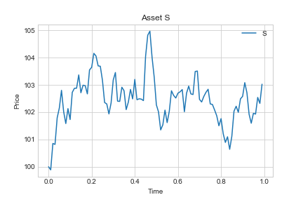
Figure 1: Asset price in a market with volatility $\sigma=0.05$.

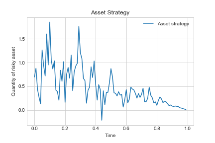
Figure 2: The quantity $(\gamma_{t})_{0\leq t\leq 1}$ of risky asset $(S_{t})_{0\leq t\leq 1}$ in a hedging strategy for an Asian market option with volatility $\sigma=0.05$.

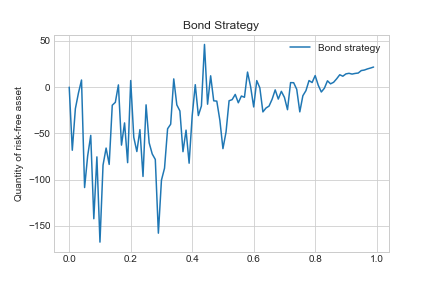
Figure 3: The quantity $(\beta_{t})_{0\leq t\leq 1}$ of riskless asset $(B_{t})_{0\leq t\leq 1}$ in a hedging strategy for an Asian market option with volatility $\sigma=0.05$.

Let us compare the value of the terminal portfolio and the payoff function for a different number of partitions $N$ with parameters $\sigma=0.1$, $S_{0}=100$, $K=50$.

Table 1: The terminal portfolio $X_{1}$ and the pauoff $f_{1}$

$N$	20	50	100	200	500	1000
$X_{1}$	74.1408	37.7123	22.76484379	184.6879	50.0242	10.220968
$f_{1}$	47.8504	49.5922	22.4617	61.5188	52.9817	6.37918036

The value of the option is calculated by the formula

$$C_{0}\approx\frac{1}{L}\sum\limits_{j=1}^{L}\left(S_{0}\sum\limits_{k=1}^{N}dt*\exp\{\sigma W_{k}(1)-\sigma^{2}t_{k}/2\}\right)_{+}.$$

Consider the simulation results for $S_{0}=100$, $t\in[0,1]$, ${L=500000}$ and $n=1000$.

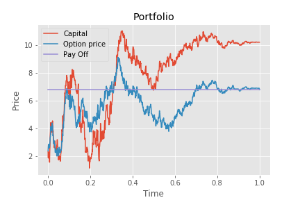
Figure 4: Graphs of option value, investor’s capital and Asian option payoff function.

In Fig. 4time changes on the abscissa axis, and corresponding values on the ordinate axis. We see that at every moment in time, the trajectory of the option value almost repeats the trajectory of investor capital, which is natural for the hedging task. The size of the terminal portfolio exceeds the payoff function, which confirms that the strategy is hedging.

Investigating the behavior of the option value depending on the initial stock price $S_{0}$, strike price $K$ and volatility $\sigma$, we obtain the following results.

Table 2: The dependence of the value of an Asian option on the volatility parameter with $K=S_{0}$

$\sigma$	0.01	0.05	0.1	0.5	1	1.5	2
$C_{0}$	0.229	1.371	2.303	11.346	22.473	32.941	42.466

Table 3: The dependence of the value of an Asian option on the volatility parameter with $K=S_{0}/2$

$\sigma$	0.01	0.05	0.1	0.5	1	1.5	2
$C_{0}$	50.115	50.201	50.107	50.055	51.669	55.832	59.443

Calculating the value of the option without costs and wiyh costs when parameters $\sigma=0.05$ and $S_{0}=100,K=70$ for a different number of portfolio revisions, we obtain the following result.

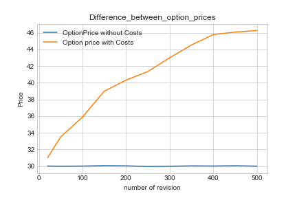
Figure 5: The value of the option in the market with transaction costs and without costs.

We have investigated the behavior of the hedging error $V_{1}^{n}-f_{1}$ with different portfolio revision numbers ”n”   and different parameters $\sigma$. Let $S_{0}=K=100$, $\kappa_{0}=0.05$.

Table 4: The hedging error when $\sigma=0.1$

$n$	20	50	100	200	500	1000
$V_{1}^{n}-f_{1}$	-0.3264	-0.1479	-0.0693	-0.0097	0.0026	0.0061

Table 5: The hedging error when $\sigma=0.9$

$n$	20	50	100	200	500	1000
$V_{1}^{n}-f_{1}$	-0.7106	-0.4065	-0.3307	-0.1938	-0.0801	-0.0213

An analysis of the numerical results showed that the value of the option increases if the strike price is less than the initial value of the stock. Volatility also affects the value of the option, it increases with increasing volatility, but not significantly. The portfolio revealed an inverse proportion between the number of risky and risk-free assets. As a result of the experiment, the influence of the number of revisions of the portfolio $n$ on the value of the option in financial markets with transaction costs was confirmed, it was revealed that with the growth of $n$ the value of the option also increases. The cost of an option in financial markets without costs does not depend on the number of “revisions”. Also, a numerical experiment showed that in markets with transaction costs, the hedging error decreases with an increase in the number of portfolio revisions. It was also revealed that hedging error is greater with high market volatility.

8 Appendix

8.1 Technical lemmas

Lemma 1

Let

$$B_{n}=\kappa_{n}\sum_{j=1}^{n}S_{t_{j}}|H(t_{j},\xi_{t_{j}},S_{t_{j}})-H(t_{j-1},\xi_{t_{j-1}},S_{t_{j}})|,$$ (25)

$$\kappa_{n}\underset{n\to\infty}{\longrightarrow}0$$

then

$${\bf P}-\lim_{n\rightarrow\infty}B_{n}=0$$ (26)

Proof

We can represent

$$H(t_{j},\xi_{t_{j}},S_{t_{j}}) =\underbrace{H(t_{j},\xi_{t_{j}},S_{t_{j}})-H(t_{j-1},\xi_{t_{j}},S_{t_{j}})}_{h_{j}}+\underbrace{H(t_{j-1},\xi_{t_{j}},S_{t_{j}})-H(t_{j-1},\xi_{t_{j-1}},S_{t_{j}})}_{h_{j}^{(1)}}$$

$$+H(t_{j-1},\xi_{t_{j-1}},S_{t_{j}}).$$

Then

$$B_{n}=D_{n}^{(t)}+D_{n}^{(x)}=\kappa_{n}\sum_{j=1}^{n}d_{j}^{(t)}+\kappa_{n}\sum_{j=1}^{n}d_{j}^{(x)},$$

where

$$d_{j}^{(t)}=S_{t_{j}}h_{j},\;\;\;\;\;\;d_{j}^{(x)}=S_{t_{j}}h_{j}^{(1)}.$$

It is necessary to show that $\forall\mu>0$

$$\lim\limits_{n\rightarrow\infty}{\bf P}(D_{n}^{(t)}>\mu)=0\;\;\;\text{and}\;\;\;\lim\limits_{n\rightarrow\infty}{\bf P}(D_{n}^{(x)}>\mu)=0.$$ (27)

Recall that

$$H(t,x,y)=\hat{G}_{y}(t,x,y)=\int\limits_{b}^{\infty}z\hat{q}(v,z)dz,$$

where $\hat{q}(v,z)$ – the density of the random density

$$\hat{\eta}_{v}=\int\limits_{0}^{v}\exp\{\hat{\sigma}W_{u}-\hat{\sigma}^{2}u/2\}du$$

and

$$b=\left(\frac{K-x}{y}\right)_{+}.$$

We introduce the stopping time

$$\tau_{0}=\inf\{t>0:\xi_{t}\geq K\}\wedge 1.$$ (28)

Clear that always $0<\tau_{0}\leq 1$ and starting from $\tau_{0}$, all coefficients $b=0$. To compensate $b$ and $S_{t}$ we introduce the following sets

$$\Gamma_{\varepsilon,M}=\{\xi_{1}>K\}\cap\{\tau_{0}\leq 1-\varepsilon\}\cap\{M^{-1}\leq\min\limits_{0\leq t\leq 1}S_{t}\leq\max\limits_{0\leq t\leq 1}S_{t}\leq M\}$$

$$\tilde{\Gamma}_{\delta,M}=\{\xi_{1}\leq K-\delta\}\cap\{M^{-1}\leq\min\limits_{0\leq t\leq 1}S_{t}\leq\max\limits_{0\leq t\leq 1}S_{t}\leq M\}$$

moreover

$$\lim\limits_{M\to\infty}\lim\limits_{\varepsilon\to 0}{\bf P}(\Gamma_{\varepsilon,M}^{c})=0,\;\;\;\;\;\lim\limits_{M\to\infty}\lim\limits_{\delta\to 0}{\bf P}(\tilde{\Gamma}_{\delta,M}^{c})=0.$$ (29)

Then we represent probabilities as

$${\bf P}(D_{n}^{(t)}>\mu) ={\bf P}(D_{n}^{(t)}>\mu,\xi_{1}>K)+{\bf P}(D_{n}^{(t)}>\mu,\xi_{1}\leq K)$$

$$\leq{\bf P}(D_{n}^{(t)}>\mu,\Gamma_{\varepsilon,M})+{\bf P}(\Gamma^{c}_{\varepsilon,M})+{\bf P}(D_{n}^{(t)}>\mu,\tilde{\Gamma}_{\delta,M})+{\bf P}(\tilde{\Gamma}^{c}_{\delta,M})$$ (30)

and

$${\bf P}(D_{n}^{(x)}>\mu) ={\bf P}(D_{n}^{(t)}>\mu,\xi_{1}>K)+{\bf P}(D_{n}^{(x)}>\mu,\xi_{1}\leq K)$$

$$\leq{\bf P}(D_{n}^{(x)}>\mu,\Gamma_{\varepsilon,M})+{\bf P}(\Gamma^{c}_{\varepsilon,M})+{\bf P}(D_{n}^{(x)}>\mu,\tilde{\Gamma}_{\delta,M})+{\bf P}(\tilde{\Gamma}^{c}_{\delta,M})$$ (31)

Taking into account Proposition 5 and Proposition 6 we obtain the equalities (27).

Proposition 5

For fixed $\varepsilon>0$ and $M>0$

$$\lim\limits_{n\rightarrow\infty}{\bf P}(D_{n}^{(t)}>\mu,\Gamma_{\varepsilon,M})=0;$$ (32)

$$\lim\limits_{n\rightarrow\infty}{\bf P}(D_{n}^{(x)}>\mu,\Gamma_{\varepsilon,M})=0.$$ (33)

Here

$$\Gamma_{\varepsilon,M}=\{\xi_{1}>K\}\cap\{\tau_{0}\leq 1-\varepsilon\}\cap\{M^{-1}\leq\min\limits_{0\leq t\leq 1}S_{t}\leq\max\limits_{0\leq t\leq 1}S_{t}\leq M\}$$

Proof

First we divide $D_{n}^{(t)}$ and $D_{n}^{(x)}$ into two amounts

$$D^{(t)}_{n} =\kappa_{n}\sum_{j=1}^{n_{1}}d^{(t)}_{j}+\kappa_{n}\sum_{j=n_{1}+1}^{n}d^{(t)}_{j},$$

$$D^{(x)}_{n} =\kappa_{n}\sum_{j=1}^{n_{1}}d^{(x)}_{j}+\kappa_{n}\sum_{j=n_{1}+1}^{n}d^{(x)}_{j},\;\;\;\;n_{1}=[(1-\varepsilon)n].$$

We choose $n_{1}$ from the condition $t_{n_{1}}\geq 1-\varepsilon$. In this case, we have

$$(t_{j})_{j=n_{1}+1}^{n}>\tau_{0}\;\;\;\text{and}\;\;\;(\xi_{t_{j}})_{j=n_{1}+1}^{n}\geq K.$$

Therefore

$$b_{j}=0,\;\;\;j=\overline{n_{1}+1,n}$$

and since

$$H(t,x,y) =\int\limits_{b}^{\infty}z\hat{q}(v,z)dz=\int\limits_{0}^{\infty}z\hat{q}(v,z)dz={\bf E}\hat{\eta}_{v}$$

$$={\bf E}\left(\int\limits_{0}^{v}\exp\{\hat{\sigma}W_{u}-\hat{\sigma}^{2}u/2\}du\right)=\int\limits_{0}^{v}{\bf E}\exp\{\hat{\sigma}W_{u}-\hat{\sigma}^{2}u/2\}du=v$$

we obtain

$$d^{(t)}_{j}=S_{t_{j}}|H(t_{j},\xi_{t_{j}},S_{t_{j}})-H(t_{j-1},\xi_{t_{j}},S_{t_{j}})|\leq M\Delta v_{j}\leq\frac{M}{n},\;\;\;j=\overline{n_{1}+1,1}$$

$$\kappa_{n}\sum_{j=n_{1}+1}^{n}d^{(t)}_{j}\underset{n\to\infty}{\longrightarrow}0$$

и

$$d^{(x)}_{j}=S_{t_{j}}|H(t_{j-1},\xi_{t_{j}},S_{t_{j}})-H(t_{j-1},\xi_{t_{j-1}},S_{t_{j}})|=0,\;\;\;\;j=\overline{n_{1}+1,1}.$$

Thus, on the set $\Gamma_{\varepsilon,M}$ we have

$$D^{(t)}_{n}=\kappa_{n}\sum_{j=1}^{n_{1}}d^{(t)}_{j};\;\;\;D^{(x)}_{n}=\kappa_{n}\sum_{j=1}^{n_{1}}d^{(x)}_{j}.$$

Next we evaluate $d^{(t)}_{j}$ on the interval $[t_{1},t_{n_{1}}]$, on which all $t_{j}<1-\varepsilon$.

$$d^{(t)}_{j} =S_{t_{j}}\bigg{|}\int\limits_{b_{t_{j}}}^{\infty}z\hat{q}(v_{j},z)dz-\int\limits_{b_{t_{j-1}}}^{\infty}z\hat{q}(v_{j-1},z)dz\bigg{|}$$

$$\leq M\int\limits_{0}^{\infty}z|\hat{q}(v_{j},z)-\hat{q}(v_{j-1},z)|dz\leq M\int\limits_{0}^{\infty}z\bigg{|}\int\limits_{v_{j-1}}^{v_{j}}\hat{q}_{v}(u,z)du\bigg{|}dz$$

$$\leq\int\limits_{0}^{1}z\bigg{|}\int\limits_{v_{j-1}}^{v_{j}}\hat{q}_{v}(u,z)du\bigg{|}dz+\int\limits_{1}^{\infty}z\bigg{|}\int\limits_{v_{j-1}}^{v_{j}}\hat{q}_{v}(u,z)du\bigg{|}dz.$$

Naking into account Proposition 4, we can estimate

$$\bigg{|}\int_{v_{j-1}}^{v_{j}}\hat{q}_{v}(u,z)du\bigg{|}\leq\frac{c}{\varepsilon^{4}}\int_{v_{j}}^{v_{j-1}}\exp\{-\theta(\ln(z/v))^{2}\}du,$$

because we can evaluate $1/v\leq 1$. If $0<z\leq 1$, then we can use a uniform estimate for $\hat{q}_{v}(v,z)$

$$\hat{q}_{v}(v,z)\leq\frac{c}{v^{4}}\leq\frac{c}{\varepsilon^{4}}$$

and if $z>1$, we use inequality $\ln(z/v)\geq\ln(z/\varepsilon)$. Then

$$\hat{q}_{v}(v,z)\leq\frac{c}{\varepsilon^{4}}\exp\left\{-\theta(\ln(z/\varepsilon))^{2}\right\}.$$

Therefore,

$$d^{(t)}_{j}\leq\frac{Mc}{2n\varepsilon^{4}}+\frac{Mc}{n\varepsilon^{4}}\int\limits_{1}^{\infty}z\exp\left\{-\theta(\ln(z/\varepsilon))^{2}\right\}dz,$$

and the integral

$$I_{1}=\int\limits_{1}^{\infty}z\exp\left\{-\theta(\ln(z/\varepsilon))^{2}\right\}dz$$

is converge. Then

$$D^{(t)}_{n}\leq M\kappa_{n}\sum_{j=1}^{n_{1}}d^{(t)}_{j}\leq\kappa_{n}\sum_{j=1}^{n_{1}}\frac{Mc}{n\varepsilon^{4}}(1/2+I_{1})=\kappa_{n}\frac{Mcn_{1}}{n\varepsilon^{4}}(1/2+I_{1})\xrightarrow[n\rightarrow\infty]{\mathbf{P}}0$$

that is

$$\lim\limits_{n\rightarrow\infty}{\bf P}(D_{n}^{(t)}>\mu,\Gamma_{\varepsilon,M})=0.$$

Let’s estimate $d^{(x)}_{j}$ on the interval $[t_{1},t_{n_{1}}]$. Since $H(t,x,y)=\int\limits_{b}^{\infty}z\hat{q}(v,z)dz$, then

$$H^{\prime}_{x}(t,x,y)(t,x,y)=-\frac{b}{y}\hat{q}(v,b)$$

and we can evaluate this derivative using Proposition 3.

$$|H_{x}(t,x,y)|\leq\frac{bq(v,b)}{y}\leq\frac{KM^{2}c}{\varepsilon^{2}}$$

We used a uniform estimate for $\hat{q}(v,b)$. Thus the derivative $H_{x}(t,x,y)$ is uniformly bounded. This means that the function $H(t,x,y)$ satisfies the conditions of Lipschitz and moreover

$$|H(t_{j-1},\xi_{t_{j}},S_{t_{j}})-H(t_{j-1},\xi_{t_{j-1}},S_{t_{j}})| \leq|H_{x}(t,x,y)||\xi_{t_{j}}-\xi_{t_{j-1}}|\leq\frac{KM^{2}с}{\varepsilon^{2}}|\xi_{t_{j}}-\xi_{t_{j-1}}|$$

$$\leq\frac{KM^{2}с}{\varepsilon^{2}}\int_{t_{j-1}}^{t_{j}}S_{u}du\leq\frac{KM^{3}с}{\varepsilon^{2}}\Delta t_{j}=\frac{KM^{3}с}{n\varepsilon^{2}}.$$

Then

$$D^{(x)}_{n}\leq\kappa_{n}M\sum_{j=1}^{n_{1}}\frac{KM^{3}с}{n\varepsilon^{2}}\leq\kappa_{n}\frac{KM^{4}cn_{1}}{n\varepsilon^{2}}\xrightarrow[n\rightarrow\infty]{\mathbf{P}}0.$$

that is

$$\lim\limits_{n\rightarrow\infty}{\bf P}(D_{n}^{(x)}>\mu,\Gamma_{\varepsilon,M})=0.$$

Proposition 6

For fixed $\delta>0$ and $M>0$

$$\lim\limits_{n\rightarrow\infty}{\bf P}(D_{n}^{(t)}>\mu,\tilde{\Gamma}_{\delta,M})=0;$$ (34)

$$\lim\limits_{n\rightarrow\infty}{\bf P}(D_{n}^{(x)}>\mu,\tilde{\Gamma}_{\delta,M})=0.$$ (35)

Here

$$\tilde{\Gamma}_{\delta,M}=\{\xi_{1}\leq K-\delta\}\cap\{M^{-1}\leq\min\limits_{0\leq t\leq 1}S_{t}\leq\max\limits_{0\leq t\leq 1}S_{t}\leq M\}$$

Proof

We can use the following estimate

$$D_{n}^{(x)}\leq\kappa_{n}M\sum_{j=1}^{n}|H_{x}(t,x,y)||\xi_{t_{j}}-\xi_{t_{j-1}}|,$$

since

$$|H_{x}(t,x,y)|\leq\frac{b\hat{q}(v,b)}{y}\leq KM^{2}\frac{c}{v^{2}}\left(\exp\left\{-\theta(\ln(b/v))^{2}\right\}{\bf 1}_{\{z>v\}}+{\bf 1}_{\{z\leq v\}}\right).$$

It’s obvious that $\xi_{t_{j}}\leq\xi_{1}\leq K-\delta$ on the set $\tilde{\Gamma}_{\delta,M}$, so

$$b_{*}=\frac{\delta}{M}\leq b_{t_{j}}\leq KM.$$

Similar to the proof of the Proposition 6 we split $D_{n}^{(x)}$ into two amounts

$$D^{(x)}_{n}=\kappa_{n}\sum_{j=1}^{n_{1}}d^{(x)}_{j}+\kappa_{n}\sum_{j=n_{1}+1}^{n}d^{(x)}_{j}.$$

If $0<v<b_{*}$, i.e. $1-b_{*}<t<1$, then we use estimate

$$|H_{x}(t,x,y)|\leq\frac{KM^{2}c}{v^{2}}\exp\left\{-\theta(\ln(b_{*}/v))^{2}\right\}.$$

If $b_{*}<v<1$, i.e. $0\leq t\leq 1-b_{*}$, then

$$|H_{x}(t,x,y)|\leq\frac{KM^{2}c}{b_{*}^{2}}.$$

Thus,

$$D^{(x)}_{n} \leq\frac{\kappa_{n}cM^{3}K}{b_{*}^{2}}\sum_{j=1}^{n_{1}}|\xi_{t_{j}}-\xi_{t_{j-1}}|+M^{3}K\kappa_{n}\sum_{j=n_{1}+1}^{n}\frac{c}{v_{j}^{2}}\exp\{-\theta(\ln(b_{*}/v_{j}))^{2}\}|\xi_{t_{j}}-\xi_{t_{j-1}}|$$

$$\leq\frac{cM^{4}Kn_{1}\kappa_{n}}{nb_{*}^{2}}+M^{4}K\kappa_{n}\sum_{j=n_{1}+1}^{n}\frac{c}{v_{j}^{2}}\exp\{-\theta(\ln(b_{*}/v_{j}))^{2}\}\Delta t_{j}$$

Note that

$$\sum_{j=n_{1}+1}^{n}\frac{c}{v_{j}^{2}}\exp\{-\theta(\ln(b_{*}/v_{j}))^{2}\}\Delta t_{j}\xrightarrow[n\rightarrow\infty]{}\int\limits_{1-b_{*}}^{1}\frac{c}{v^{2}}\exp\{-\theta(\ln(b_{*}/v))^{2}\}dt.$$

Consider

$$J=\int\limits_{1-b_{*}}^{1}\frac{c}{v^{2}}\exp\{-\theta(\ln(b_{*}/v))^{2}\}dt.$$

Given that $v=1-t$, make a variable change

$$\tilde{a}=\frac{1}{1-t},$$

then $dt=d\tilde{a}/\tilde{a}^{2}$ and we obtain

$$J =\int_{1/b_{*}}^{\infty}\tilde{a}^{2}\exp\{-\theta(\ln(b_{*}\tilde{a}))^{2}\}d\tilde{a}=\frac{1}{b_{*}}\int_{1}^{\infty}\exp\{-\theta(\ln\hat{a})^{2}\}d\hat{a}$$

$$=\frac{1}{b_{*}}\int_{0}^{\infty}\exp\{-\theta(\ln y)^{2}+y\}dy$$

The last integral $I_{2}=\frac{1}{b_{*}}\int_{0}^{\infty}\exp\{-\theta(\ln y)^{2}+y\}dy$ converges. Thus,

$$D_{n}^{(x)}\leq\kappa_{n}cKM^{4}\left(\frac{n_{1}}{nb_{*}^{2}}+I_{2}\right)\xrightarrow[n\rightarrow\infty]{{\bf P}}0$$

and

$$\lim\limits_{n\rightarrow\infty}{\bf P}(D_{n}^{(x)}>\mu,\tilde{\Gamma}_{\delta,M})=0.$$

Consider

$$D_{n}^{(t)}=\kappa_{n}\sum_{j=1}^{n}d_{j}^{(t)}.$$

Recall that on the set $\tilde{\Gamma}_{\delta,M}$ all $\xi_{t_{j}}\leq\xi_{1}\leq K-\delta$, then

$$b_{t_{j}}=\frac{K-\xi_{t_{j}}}{S_{t_{j}}}\geq b_{*},\;\;\;\delta_{1}=\frac{\delta}{M}.$$

Similarly, we evaluate $d_{j}^{(t)}$.

$$d_{j}^{(t)} =S_{t_{j}}\bigg{|}\int_{b_{t_{j}}}^{\infty}z\hat{q}(v_{j},z)dz-\int_{b_{t_{j-1}}}^{\infty}z\hat{q}(v_{j-1},z)dz\bigg{|}\leq M\int_{b_{*}}^{\infty}z\bigg{|}\int_{v_{j-1}}^{v_{j}}q_{v}(u,z)du\bigg{|}dz$$

$$\leq M\int_{b_{*}}^{\infty}z\left(\int_{v_{j}}^{v_{j-1}}|\hat{q}_{v}(u,z)|du\right)dz=M\int_{v_{j}}^{v_{j-1}}\left(\int_{b_{*}}^{\infty}z|\hat{q}_{v}(u,z)|dz\right)du$$

Next, we use the estimate for the derivative of the density $\hat{q}_{v}(u,z)$, obtained in Proposition 4,

$$\int_{v_{j}}^{v_{j-1}}\left(\int_{b_{*}}^{\infty}z|\hat{q}_{v}(u,z)|dz\right)du\leq\int_{v_{j}}^{v_{j-1}}\frac{c}{u^{4}}\left(\int_{b_{*}}^{\infty}z\exp\{-\theta(\ln(z/u))^{2}\}dz\right)du$$

Make the change of variable $y=z/u$

$$\int_{v_{j}}^{v_{j-1}}\left(\int_{b_{*}}^{\infty}z|\hat{q}_{v}(u,z)|dz\right)du \leq\int_{v_{j}}^{v_{j-1}}\frac{c}{u^{2}}\left(\int_{b_{*}/u}^{\infty}y\exp\{-\theta(\ln y)^{2}\}dy\right)du$$

$$=\int_{v_{j}}^{v_{j-1}}\frac{c}{u^{2}}I(u)du$$

We consider separately the integral

$$I(u)=\int_{b_{*}/u}^{\infty}y\exp\{-\theta(\ln y)^{2}\}dy.$$

We use the change of variable $x=\ln y$ and obtain

$$I(u)=\int_{\ln(b_{*}/u)}^{\infty}\exp\{-\theta x^{2}+2x\}dx.$$

Select a parabola so that $c_{*}=\sup\limits_{x}(\exp\{-\theta x^{2}/2+2x\})$, then we can write an estimate

$$I(u) \leq c_{*}\int_{\ln(b_{*}/u)}^{\infty}\exp\{-\theta x^{2}/2\}dx=c_{*}\int_{\ln(b_{*}/u)}^{\infty}\exp\left\{-\theta x^{2}/4\right\}\exp\left\{-\theta x^{2}/4\right\}dx$$

$$\leq c_{*}\exp\left\{-\theta(\ln(b_{*}/u))^{2}/4\right\}\int_{-\infty}^{\infty}\exp\left\{-\theta x^{2}/4\right\}dx$$

If $u\geq b_{*}$, then

$$I(v)\leq c_{*}\int_{-\infty}^{+\infty}\exp\left\{-\theta x^{2}/4\right\}dx.$$

If $0<u<b_{*}$, then $\ln(b_{*}/u)>0$ and we can evaluate the integral as

$$I(u)\leq c_{*}\exp\left\{-\theta(\ln(b_{*}/u))^{2}/4\right\}\int_{0}^{\infty}\exp\left\{-\theta x^{2}/4\right\}dx.$$

Then

$$d^{(t)}_{j} \leq M\int_{v_{j}}^{v_{j-1}}\frac{c}{u^{2}}I(u)du\leq M\int_{0}^{1}\frac{c}{u^{2}}I(u)du$$

$$\leq MJ_{1}\int_{0}^{b_{*}}\exp\left\{-\theta(\ln(b_{*}/u))^{2}/4\right\}\frac{c}{u^{2}}du+MJ_{2}\int_{b_{*}}^{1}\frac{c}{u^{2}}du,$$

with constants

$$J_{1}=c_{*}\int_{0}^{+\infty}\exp\left\{-\theta x^{2}/4\right\}dx;\;\;\;\;\;J_{2}=c_{*}\int_{-\infty}^{+\infty}\exp\left\{-\theta x^{2}/4\right\}dx.$$

It is clear that the integral

$$I_{1}=\int_{b_{*}}^{1}\frac{c}{u^{2}}du$$

converges. Consider the integral

$$I_{2}=\int_{0}^{b_{*}}\exp\left\{-\theta(\ln(b_{*}/u))^{2}/4\right\}\frac{c}{u^{2}}du.$$

Let’s make a change $y=b_{*}/u$, then a change $z=\ln y$, so

$$I_{2}=\frac{c}{b_{*}^{2}}\int_{1}^{\infty}\exp\left\{-\theta(\ln y)^{2}/4\right\}dy=\frac{c}{b_{*}^{2}}\int_{1}^{\infty}\exp\left\{-\theta z^{2}/4+z\right\}dz<+\infty$$

Thus, it was shown that $d^{(t)}_{j}$ is limited by some constant

$$d^{(t)}_{j}\leq l(M,J_{1},J_{2},I_{1},I_{2}).$$

Therefore,

$$D^{(t)}_{n}=\kappa_{n}\sum_{j=1}^{n}d^{(t)}_{j}\leq\frac{\kappa_{n}l(M,J_{1},J_{2},I_{1},I_{2})}{n}\xrightarrow[n\rightarrow\infty]{{\bf P}}0$$

and we get that

$$\lim\limits_{n\rightarrow\infty}{\bf P}(D_{n}^{(t)}>\mu,\tilde{\Gamma}_{\delta,M})=0.$$

.

Lemma 2

Let

$$D_{n}^{(y)}=\kappa_{n}\sum_{j=1}^{n}d_{j}^{(y)},$$

where

$$d_{j}^{(y)}=S_{t_{j}}|H(t_{j-1},\xi_{t_{j-1}},S_{t_{j}})-H(t_{j-1},\xi_{t_{j-1}},S_{t_{j-1}})-H_{y}(t_{j-1},\xi_{t_{j-1}},S_{t_{j-1}})(S_{t_{j}}-S_{t_{j-1}})|.$$

Then

$${\bf P}-\lim_{n\rightarrow\infty}D_{n}^{(y)}=0.$$ (36)

Proof

Represent $d_{j}^{(y)}$ as

$$d_{j}^{(y)} \leq\bigg{|}S_{t_{j}}\int\limits_{S_{t_{j-1}}}^{S_{t_{j}}}(H_{y}(t_{j-1},\xi_{t_{j-1}},u)-H_{y}(t_{j-1},\xi_{t_{j-1}},S_{t_{j-1}}))du\bigg{|}$$

$$\leq\bigg{|}S_{t_{j}}\int\limits_{S_{t_{j-1}}}^{S_{t_{j}}}\left(\int\limits_{S_{t_{j-1}}}^{u}H_{yy}(t_{j-1},\xi_{t_{j-1}},a)da\right)du\bigg{|}.$$ (37)

Let’s find the derivative $H_{yy}(t,x,y)$. Recall that

$$H(t,x,y)=\int\limits_{b}^{\infty}z\hat{q}(v,z)dz\;\;\;\text{и}\;\;\;b=\frac{(K-x)_{+}}{y}.$$

If $x\geq K$, then $H(t,x,y)=1-t$ and $H_{y}(t,x,y)=H_{yy}(t,x,y)=0$. If $x<K$, then

$$H_{y}(t,x,y)=-b\hat{q}(v,b)b^{\prime}_{y}=\frac{b^{2}}{y}\hat{q}(v,b)=\frac{(K-x)^{2}}{y^{3}}\hat{q}(v,b)$$

and

$$H_{yy}(t,x,y) =-\frac{3(K-x)^{2}}{y^{4}}\hat{q}(v,b)+\frac{(K-x)^{2}}{y^{3}}\hat{q}_{z}(v,b)b^{\prime}_{y}$$

$$=-\frac{3b^{2}}{y^{2}}\hat{q}(v,b)-\frac{b^{3}}{y^{2}}\hat{q}_{z}(v,b)$$

It is necessary to show that for $\forall\mu>0$

$$\lim\limits_{n\rightarrow\infty}{\bf P}(D_{n}^{(y)}>\mu)=0.$$

As before in the proof of Lemma 1 we introduce the stopping time $\tau_{0}$ and sets

$$\Gamma_{\varepsilon,M}=\{\xi_{1}>K\}\cap\{\tau_{0}\leq 1-\varepsilon\}\cap\{M^{-1}\leq\min\limits_{0\leq t\leq 1}S_{t}\leq\max\limits_{0\leq t\leq 1}S_{t}\leq M\}$$

$$\Gamma_{\delta,M}=\{\xi_{1}\leq K-\delta\}\cap\{M^{-1}\leq\min\limits_{0\leq t\leq 1}S_{t}\leq\max\limits_{0\leq t\leq 1}S_{t}\leq M\},$$

with

$$\lim\limits_{M\to\infty}\lim\limits_{\varepsilon\to 0}{\bf P}(\Gamma_{\varepsilon,M}^{c})=0,\;\;\;\;\;\lim\limits_{M\to\infty}\lim\limits_{\delta\to 0}{\bf P}(\Gamma_{\delta,M}^{c})=0.$$ (38)

Represent the probability ${\bf P}(D_{n}^{(y)}>\mu)$ as

$${\bf P}(D_{n}^{(y)}>\mu) ={\bf P}(D_{n}^{(y)}>\mu,\xi_{1}>K)+{\bf P}(D_{n}^{(y)}>\mu,\xi_{1}\leq K)$$

$$\leq{\bf P}(D_{n}^{(y)}>\mu,\Gamma_{\varepsilon,M})+{\bf P}(\Gamma_{\varepsilon,M}^{c})+{\bf P}(D_{n}^{(y)}>\mu,\Gamma_{\delta,M})+{\bf P}(\Gamma_{\delta,M}^{c}).$$

Consider ${\bf P}(D_{n}^{(y)}>\mu,\Gamma_{\varepsilon,M})$. Analogically we split $D_{n}^{(y)}$ into two sums

$$D_{n}^{(y)}=\kappa_{n}\sum_{j=1}^{n_{1}}d^{(y)}_{j}+\kappa_{n}\sum_{j=n_{1}+1}^{n}d^{(y)}_{j},$$

where $n_{1}=[(1-\varepsilon)n]$, i.e. $t_{n_{1}}\leq 1-\varepsilon$. Starting from $j=n_{1}+1$ all moments $t_{j}>\tau_{0}$ and $\xi_{t_{j}}\geq K$. So, $b_{t_{j}}=0$ and $d^{(y)}_{j}=0$. Thus,

$$D_{n}^{(y)} =\kappa_{n}\sum_{j=1}^{n_{1}}d^{(2)}_{j}$$

$$\leq M\kappa_{n}\sum_{j=1}^{n_{1}}|H(t_{j-1},\xi_{t_{j-1}},S_{t_{j}})-H(t_{j-1},\xi_{t_{j-1}},S_{t_{j-1}})-H_{y}(t_{j-1},\xi_{t_{j-1}},S_{t_{j-1}})(S_{t_{j}}-S_{t_{j-1}})|$$

$$\leq M\kappa_{n}\sum_{j=1}^{n_{1}}\bigg{|}\int\limits_{S_{t_{j-1}}}^{S_{t_{j}}}\left(\int\limits_{S_{t_{j-1}}}^{u}H_{yy}(t_{j-1},\xi_{t_{j-1}},a)da\right)du\bigg{|}.$$

Using Proposition 3, we can estimate $1/v\leq 1$ and

$$|H_{yy}(t,x,y)| =\bigg{|}\frac{3b^{2}}{y^{2}}\hat{q}(v,b)+\frac{b^{3}}{y^{2}}\hat{q}_{z}(v,b)\bigg{|}$$

$$\leq\bigg{|}\frac{3b^{2}}{y^{2}}\frac{c}{v^{2}}\exp\{-\theta(\ln(b/v))^{2}\}+\frac{b^{3}}{y^{2}}\frac{c}{v^{4}}\exp\{-\theta(\ln(b/v))^{2}\}\bigg{|}.$$

On the set $\Gamma_{\varepsilon,M}$ we change the exponent by 1 and $v=1-t$ by $\varepsilon$, also take into account that $b\leq K/y\leq KM$. For some constant $c_{*}$ we have

$$|H_{yy}(t,x,y)|\leq\frac{c}{y^{4}\varepsilon^{2}}+\frac{c}{y^{5}\varepsilon^{4}}\leq\frac{c_{*}M^{5}}{\varepsilon^{4}}.$$

Then

$$d^{(y)}_{j} \leq M\bigg{|}\int\limits_{S_{t_{j-1}}}^{S_{t_{j}}}\left(\int\limits_{S_{t_{j-1}}}^{u}H_{yy}(t_{j-1},\xi_{t_{j-1}},a)da\right)du\bigg{|}$$

$$\leq M^{6}\frac{c_{*}}{\varepsilon^{4}}\bigg{|}\int\limits_{S_{t_{j-1}}}^{S_{t_{j}}}(u-S_{t_{j-1}})du\bigg{|}=\frac{cM^{6}}{\varepsilon^{4}}|S_{t_{j}}-S_{t_{j-1}}|^{2}$$

Note that

$${\bf E}(S_{t_{j}}-S_{t_{j-1}})^{2}=\sigma^{2}{\bf E}\int\limits_{t_{j-1}}^{t_{j}}S_{u}^{2}du\leq\sigma^{2}e^{\sigma^{2}}(t_{j}-t_{j-1})=\frac{c}{n},$$

Since

$${\bf E}S_{u}^{2}={\bf E}\exp\{2\sigma W_{u}-\sigma^{2}u\}=e^{\sigma^{2}u}\leq e^{\sigma^{2}}.$$

Therefore,

$$D^{(y)}_{n}\leq M\kappa_{n}\sum_{j=1}^{n_{1}}\frac{cM^{6}}{\varepsilon^{4}}|S_{t_{j}}-S_{t_{j-1}}|^{2}$$

Let $\tilde{c}=cM^{7}/\varepsilon^{4}$, then

$${\bf P}\left(D_{n}^{(y)}>\mu,\Gamma_{\varepsilon,M}\right) \leq{\bf P}\left(\kappa_{n}\tilde{c}\sum_{j=1}^{n_{1}}|S_{t_{j}}-S_{t_{j-1}}|^{2}>\mu,\Gamma_{\varepsilon,M}\right)$$

$$\leq{\bf P}\left(\kappa_{n}\tilde{c}\sum_{j=1}^{n_{1}}|S_{t_{j}}-S_{t_{j-1}}|^{2}>\mu\right)$$

Further, by Chebyshev’s inequality, we obtain

$${\bf P}(\kappa_{n}\tilde{c}\sum_{j=1}^{n_{1}}|S_{t_{j}}-S_{t_{j-1}}|^{2}>\mu)\leq\frac{\kappa_{n}\tilde{c}\sum_{j=1}^{n_{1}}{\bf E}|S_{t_{j}}-S_{t_{j-1}}|^{2}}{\mu}\xrightarrow[n\rightarrow\infty]{{\bf P}}0.$$

Thus,

$$\lim\limits_{n\rightarrow\infty}{\bf P}(D_{n}^{(y)}>\mu,\Gamma_{\varepsilon,M})=0.$$ (39)

Consider ${\bf P}(D_{n}^{(y)}>\mu,\Gamma_{\delta,M})$. On the set $\Gamma_{\delta,M}$

$$b_{*}=\frac{\delta}{M}\leq b\leq KM,$$

then

$$|H_{yy}(t,x,y)| =\bigg{|}\frac{3b^{2}}{y^{2}}\hat{q}(v,b)+\frac{b^{3}}{y^{2}}\hat{q}_{z}(v,b)\bigg{|}\leq K^{3}M^{5}|\hat{q}(v,b)+\hat{q}_{z}(v,b)|$$

$$\leq K^{3}M^{5}\bigg{|}\frac{c}{v^{4}}\exp\left\{-\theta(\ln(b/v))^{2}\right\}\bigg{|}\leq K^{3}M^{5}\bigg{|}\frac{c}{v^{4}}\exp\left\{-\theta(\ln(b_{*}/v))^{2}\right\}\bigg{|}.$$

Let $\tilde{c}=K^{3}M^{5}c$. By making a variable change $z=\ln(b_{*}/v)$, we obtain

$$|H_{yy}(t,x,y)| =\frac{\tilde{c}}{b_{*}^{4}}\left(\frac{b_{*}}{v}\right)^{4}\exp\left\{-\theta(\ln(b_{*}/v))^{2}\right\}\leq\frac{\tilde{c}}{b_{*}^{4}}\exp\{-\theta z^{2}+4z\}$$

$$\leq\frac{\tilde{c}}{b_{*}^{4}}\exp\{\sup\limits_{z\in{\mathbb{R}}}(-\theta z^{2}+4z)\}=\frac{\tilde{c}}{b_{*}^{4}}$$

Then

$$d_{j}^{(y)}\leq\frac{\tilde{c}}{b_{*}^{4}}|S_{t_{j}}-S_{t_{j-1}}|^{2}$$

So,

$$D_{n}^{(y)}\leq\kappa_{n}\frac{\tilde{c}}{b_{*}^{4}}\sum_{j=1}^{n}|S_{t_{j}}-S_{t_{j-1}}|^{2}$$

Similarly to the first part of the proof by Chebyshev inequality, we obtain

$${\bf P}(D_{n}^{(y)}>\mu,\Gamma_{\delta,M})\leq\frac{\kappa_{n}c\sum_{j=1}^{n}{\bf E}|S_{t_{j}}-S_{t_{j-1}}|^{2}}{\mu}\xrightarrow[n\rightarrow\infty]{}0.$$

Thus,

$$\lim\limits_{n\rightarrow\infty}{\bf P}(D_{n}^{(y)}>\mu,\Gamma_{\delta,M})=0.$$ (40)

As a result, from the expressions (38),(39) and (40) we obtain (36).

Lemma 3

Let $\beta(t)$ – continuous consistent function almost surely. Then

$$\frac{1}{\sqrt{n}}\sum_{j=1}^{n}\beta(t_{j-1})|S_{t_{j}}-S_{t_{j-1}}|\xrightarrow[n\rightarrow\infty]{\mathbf{P}}\sqrt{\frac{2}{\pi}}\sigma\int_{0}^{1}S_{t}\beta(t)dt.$$

Proof

All auxiliary constants will be denoted by the letter $c$. We single out the martingale term

$$\frac{1}{\sqrt{n}}\sum_{j=1}^{n}\beta(t_{j-1})|S_{t_{j}}-S_{t_{j-1}}|=\frac{1}{\sqrt{n}}\sum_{j=1}^{n}\beta(t_{j-1})\mathbf{E}\left(|S_{t_{j}}-S_{t_{j-1}}|\bigg{|}\mathcal{F}_{t_{j-1}}\right)+\frac{1}{\sqrt{n}}M_{n},$$ (41)

where

$$M_{n}=\sum_{j=1}^{n}\eta_{j},$$

$$\eta_{j}=\beta(t_{j-1})|S_{t_{j}}-S_{t_{j-1}}|-\mathbf{E}\left(\beta(t_{j-1})|S_{t_{j}}-S_{t_{j-1}}|\bigg{|}\mathcal{F}_{t_{j-1}}\right).$$

In Proposition 7 we have established that

$$\frac{1}{\sqrt{n}}M_{n}\xrightarrow[n\rightarrow\infty]{\mathbf{P}}0.$$

Now we consider the first term of the equality (41). It’s clear that

$$S_{t_{j}}-S_{t_{j-1}}=\sigma\int_{t_{j-1}}^{t_{j}}S_{u}dW_{u},$$

so

$$\beta(t_{j-1})\mathbf{E}\left(|S_{t_{j}}-S_{t_{j-1}}|\bigg{|}\mathcal{F}_{t_{j-1}}\right) =\sigma\beta(t_{j-1})\mathbf{E}\left(\bigg{|}\int_{t_{j-1}}^{t_{j}}S_{u}dW_{u}\bigg{|}\bigg{|}\mathcal{F}_{t_{j-1}}\right)$$

$$=\sigma\beta(t_{j-1})\mathbf{E}\left(\bigg{|}\int_{t_{j-1}}^{t_{j}}\left[S_{t_{j-1}}+(S_{u}-S_{t_{j-1}})\right]dW_{u}\bigg{|}\bigg{|}\mathcal{F}_{t_{j-1}}\right)$$

$$=\sigma\beta(t_{j-1})\mathbf{E}\left(\bigg{|}S_{t_{j-1}}(W_{t_{j}}-W_{t_{j-1}})+\int_{t_{j-1}}^{t_{j}}(S_{u}-S_{t_{j-1}})dW_{u}\bigg{|}\bigg{|}\mathcal{F}_{t_{j-1}}\right).$$

Introduse the notation

$$g_{j}=\int_{t_{j-1}}^{t_{j}}(S_{u}-S_{t_{j-1}})dW_{u}.$$ (42)

Then

$$\beta(t_{j-1})\mathbf{E}\left(|S_{t_{j}}-S_{t_{j-1}}|\bigg{|}\mathcal{F}_{t_{j-1}}\right) =\sigma\beta(t_{j-1})\mathbf{E}\left(\bigg{|}S_{t_{j-1}}\Delta W_{t_{j}}+g_{j}\bigg{|}\bigg{|}\mathcal{F}_{t_{j-1}}\right)$$

$$=\sigma\beta(t_{j-1})\mathbf{E}\left(\bigg{|}S_{t_{j-1}}\Delta W_{t_{j}}\bigg{|}\bigg{|}\mathcal{F}_{t_{j-1}}\right)+\sigma\beta(t_{j-1})\mathbf{E}\left(\nu_{j}\bigg{|}\mathcal{F}_{t_{j-1}}\right)$$

$$=\sigma\sqrt{\frac{2}{\pi}}\beta(t_{j-1})|S_{t_{j-1}}|\frac{1}{\sqrt{n}}+\sigma\beta(t_{j-1})\mathbf{E}\left(\nu_{j}\bigg{|}\mathcal{F}_{t_{j-1}}\right),$$ (43)

where

$$\nu_{j}=\bigg{|}S_{t_{j-1}}\Delta W_{t_{j}}+g_{j}\bigg{|}-\bigg{|}S_{t_{j-1}}\Delta W_{t_{j}}\bigg{|}.$$

By module property $\big{|}|a|-|b|\big{|}\leq|a-b|$ we have

$$|\nu_{j}|=\bigg{|}\bigg{|}S_{t_{j-1}}\Delta W_{t_{j}}+g_{j}\bigg{|}-\bigg{|}S_{t_{j-1}}\Delta W_{t_{j}}\bigg{|}\bigg{|}\leq|g_{j}|.$$ (44)

By the equality (42) and Jensen’s inequalities we get

$$\mathbf{E}\left(|g_{j}|\big{|}\mathcal{F}_{t_{j-1}}\right) =\mathbf{E}\left(\bigg{|}\int_{t_{j-1}}^{t_{j}}(S_{u}-S_{t_{j-1}})dW_{u}\bigg{|}\bigg{|}\mathcal{F}_{t_{j-1}}\right)=\sqrt{\left(\mathbf{E}\left(\bigg{|}\int_{t_{j-1}}^{t_{j}}(S_{u}-S_{t_{j-1}})dW_{u}\bigg{|}\bigg{|}\mathcal{F}_{t_{j-1}}\right)\right)^{2}}$$

$$\leq\sqrt{\mathbf{E}\left(\left(\int_{t_{j-1}}^{t_{j}}(S_{u}-S_{t_{j-1}})dW_{u}\right)^{2}\bigg{|}\mathcal{F}_{t_{j-1}}\right)}=\sqrt{\mathbf{E}\left(\int_{t_{j-1}}^{t_{j}}(S_{u}-S_{t_{j-1}})^{2}du\bigg{|}\mathcal{F}_{t_{j-1}}\right)}$$

$$=\sqrt{\int_{t_{j-1}}^{t_{j}}\mathbf{E}\left((S_{u}-S_{t_{j-1}})^{2}\bigg{|}\mathcal{F}_{t_{j-1}}\right)du}.$$

For the integrand we can write the estimate

$$\mathbf{E}\left((S_{u}-S_{t_{j-1}})^{2}\bigg{|}\mathcal{F}_{t_{j-1}}\right)\leq c^{2}S^{2}_{t_{j-1}}(u-t_{j-1})$$ (45)

This estimate is valid by virtue of the following reasoning.

$$\mathbf{E}\left((S_{u}-S_{t_{j-1}})^{2}\bigg{|}\mathcal{F}_{t_{j-1}}\right) =\mathbf{E}\left(\left(\sigma\int_{t_{j-1}}^{u}S_{v}dW_{v}\right)^{2}\bigg{|}\mathcal{F}_{t_{j-1}}\right)=\sigma^{2}\mathbf{E}\left(\int_{t_{j-1}}^{u}S^{2}_{v}dv\bigg{|}\mathcal{F}_{t_{j-1}}\right)$$

$$=\sigma^{2}\int_{t_{j-1}}^{u}\mathbf{E}\left(S^{2}_{v}\bigg{|}\mathcal{F}_{t_{j-1}}\right)dv.$$ (46)

By definition of a risky asset in this model, we have

$$S_{v}=S_{0}\exp\{\sigma W_{v}-v\sigma^{2}/2\}.$$

Obviously, the following equality holds.

$$S^{2}_{v}=S_{t_{j-1}}\exp\{2\sigma(W_{v}-W_{t_{j-1}})-\sigma^{2}(v-t_{j-1})\}.$$

Then

$$\mathbf{E}\left(S^{2}_{v}\bigg{|}\mathcal{F}_{t_{j-1}}\right) =S^{2}_{t_{j-1}}\mathbf{E}\left(\exp\{2\sigma(W_{v}-W_{t_{j-1}})-\sigma^{2}(v-t_{j-1})\}\bigg{|}\mathcal{F}_{t_{j-1}}\right)$$

$$=S^{2}_{t_{j-1}}\mathbf{E}\left(\exp\{2\sigma\sqrt{v-t_{j-1}}\eta-\sigma^{2}(v-t_{j-1})\}\right)=S^{2}_{t_{j-1}}\exp\{\sigma^{2}(v-t_{j-1})\}$$

$$\leq S^{2}_{t_{j-1}}\exp\{\sigma(t_{j}-t_{j-1})\}\leq S^{2}_{t_{j-1}}e,$$

where $\eta\sim N(0,1)$. Substituting the last inequality into(8.1), we get an estimate (45). Then

$$\mathbf{E}\left(|g_{j}|\big{|}\mathcal{F}_{t_{j-1}}\right)\leq c\sqrt{S^{2}_{t_{j-1}}\int_{t_{j-1}}^{t_{j}}(u-t_{j-1})du}=\frac{c}{n}S_{t_{j-1}}.$$ (47)

Taking into account the equality (8.1), rewrite (41) without martingale term

$$\frac{1}{\sqrt{n}}\sum_{j=1}^{n}\beta(t_{j-1})|S_{t_{j}}-S_{t_{j-1}}|=\sigma\sqrt{\frac{2}{\pi}}\sum_{j=1}^{n}\beta(t_{j-1})\frac{1}{n}S_{t_{j-1}}+\frac{\sigma}{\sqrt{n}}\sum_{j=1}^{n}\beta(t_{j-1})\mathbf{E}\left(|\nu_{j}|\bigg{|}\mathcal{F}_{t_{j-1}}\right).$$

We note here that due to inequalities (44) and (47)

$$\frac{\sigma}{\sqrt{n}}\sum_{j=1}^{n}\beta(t_{j-1})\mathbf{E}\left(|\nu_{j}|\bigg{|}\mathcal{F}_{t_{j-1}}\right)\leq\frac{\sigma}{\sqrt{n}}\sum_{j=1}^{n}|\beta(t_{j-1})|\mathbf{E}\left(|g_{j}|\bigg{|}\mathcal{F}_{t_{j-1}}\right)\leq\frac{c\sigma}{n\sqrt{n}}\sum_{j=1}^{n}|\beta(t_{j-1})|S_{t_{j-1}}.$$

Since

$$\frac{1}{n}\sum_{j=1}^{n}|\beta(t_{j-1})|S_{t_{j-1}}\xrightarrow[n\rightarrow\infty]{}\int\limits_{0}^{1}|\beta(t)|S_{t}dt\text{\;\;\;\;\;п.н.},$$

then

$$\frac{c\sigma}{\sqrt{n}}\int\limits_{0}^{1}|\beta(t)|S_{t}dt\xrightarrow[n\rightarrow\infty]{\mathbf{P}}0.$$

Hence, Следовательно, in respect Proposition 7, we obtain

$$\frac{1}{\sqrt{n}}\sum_{j=1}^{n}\beta(t_{j-1})|S_{t_{j}}-S_{t_{j-1}}|\xrightarrow[n\rightarrow\infty]{\mathbf{P}}\sigma\sqrt{\frac{2}{\pi}}\int_{0}^{1}\beta(t)S_{t}dt.$$

The lemma is proved.

Proposition 7

Let $M_{n}=\sum_{j=1}^{n}\eta_{j}$, where

$$\eta_{j}=\beta(t_{j-1})|S_{t_{j}}-S_{t_{j-1}}|-\mathbf{E}\left(\beta(t_{j-1})|S_{t_{j}}-S_{t_{j-1}}|\bigg{|}\mathcal{F}_{t_{j-1}}\right).$$

For an arbitrary continuous consistent function $\beta(t),0\leq t\leq 1$

$$\frac{1}{\sqrt{n}}M_{n}\xrightarrow[n\rightarrow\infty]{\mathbf{P}}0.$$ (48)

Proof

We consider two cases. In the first case, suppose that for some constant $L$

$$\sup_{0\leq t\leq 1}|\beta(t)|\leq L.$$

By virtue of the martingality property, we obtain

$${\bf E}(M_{n})^{2}=\mathbf{E}\sum_{j=1}^{n}\eta^{2}_{j}=\sum_{j=1}^{n}\mathbf{E}\mathbf{E}(\eta^{2}_{j}|\mathcal{F}_{t_{j-1}})=\mathbf{E}\sum_{j=1}^{n}\mathbf{E}(\eta^{2}_{j}|\mathcal{F}_{t_{j-1}}).$$ (49)

Introduce the notation $\eta_{j}=\beta(t_{j-1})\varsigma_{j}$, where

$$\varsigma_{j}=|S_{t_{j}}-S_{t_{j-1}}|-\mathbf{E}\left(|S_{t_{j}}-S_{t_{j-1}}|\big{|}\mathcal{F}_{t_{j-1}}\right).$$

Then

$$\mathbf{E}(\eta^{2}_{j}|\mathcal{F}_{t_{j-1}})=\beta^{2}(t_{j-1})\mathbf{E}(\varsigma^{2}_{j}|\mathcal{F}_{t_{j-1}})\leq L^{2}\mathbf{E}(|S_{t_{j}}-S_{t_{j-1}}|^{2}\big{|}\mathcal{F}_{t_{j-1}})\leq L^{2}S^{2}_{t_{j-1}}\Delta\frac{2}{\pi}.$$

Then we can evaluate the equality (49)

$$\mathbf{E}(M_{n})^{2}\leq L^{2}\mathbf{E}\sum_{j=1}^{n}S^{2}_{t_{j-1}}\Delta\frac{2}{\pi}=L^{2}\frac{2}{\pi n}\sum_{j=1}^{n}\mathbf{E}S^{2}_{t_{j-1}}\leq c^{2}.$$

Therefore, we obtain

$$\mathbf{E}\frac{1}{\sqrt{n}}|M_{n}|=\frac{1}{\sqrt{n}}\mathbf{E}|M_{n}|\leq\frac{1}{\sqrt{n}}(\mathbf{E}M_{n}^{2})^{1/2}\leq\frac{c}{\sqrt{n}}\xrightarrow[n\rightarrow\infty]{\mathbf{P}}0$$ (50)

In the second case, we assume that $\beta(t)$ – continuous function. We introduce the stopping time

$$\tau_{L}=\inf\{t\geq 0:|\beta(t)|\geq L\}\wedge 1.$$

For continuous function $\beta(t)$ the following equality holds

$$\mathbf{P}(\max_{0\leq t\leq 1}|\beta(t)|<\infty)=1.$$

It means that $\beta(t)$ is limited and therefore,

$$\mathbf{P}(\tau_{L}<1)\xrightarrow[L\rightarrow\infty]{}0.$$ (51)

To prove convergence (48), it must be shown that the next probability is zero.

$$\mathbf{P}\left(\frac{1}{\sqrt{n}}|M_{n}|>\delta\right)=\mathbf{P}\left(\frac{1}{\sqrt{n}}|M_{n}|>\delta,\tau_{L}=1\right)+\mathbf{P}\left(\frac{1}{\sqrt{n}}|M_{n}|>\delta,\tau_{L}<1\right).$$

On the set $\{\tau_{L}=1\}$

$$\beta(t)=\tilde{\beta}_{L}(t),$$

where

$$\tilde{\beta}_{L}(t)=\beta(t){\bf 1}_{\{|\beta(t)|\leq L\}}$$

and

$$M_{n}=\tilde{M}_{n}^{(L)}=\sum_{j=1}^{n}\tilde{\beta}_{L}(t_{j-1})\varsigma_{j}.$$

Thus, we found ourselves in the conditions of the first case considered above. Therefore,

$$\mathbf{P}\left(\frac{1}{\sqrt{n}}|M_{n}|>\delta,\tau_{L}=1\right) =\mathbf{P}\left(\frac{1}{\sqrt{n}}|\tilde{M}_{n}^{(L)}|>\delta,\tau_{L}=1\right)$$

$$\leq\mathbf{P}\left(\frac{1}{\sqrt{n}}|\tilde{M}_{n}^{(L)}|>\delta\right)\leq\frac{1}{\delta\sqrt{n}}\mathbf{E}|\tilde{M}_{n}^{(L)}|.$$

By (50), last expectation tends to zero. Then $\forall L>1$

$$\lim_{n\rightarrow\infty}\mathbf{P}\left(\frac{1}{\sqrt{n}}|M_{n}|>\delta\right) =\lim_{n\rightarrow\infty}\left(\mathbf{P}\left(\frac{1}{\sqrt{n}}|\tilde{M}_{n}^{(L)}|>\delta\right)+\mathbf{P}(\tau_{L}<1)\right)$$

$$\leq\mathbf{P}(\tau_{L}<1).$$

Pass to the limit by $L\to\infty$, with (51) we obtain (48).

8.2 Proof of the density properties

Proof

(Proposition 3)

We need to look at the asymptotic behavior $q(v,z)$ when $v\rightarrow 0$ and $z>0$ is fixed. To obtain an upper estimate for the density $q(v,z)$, it is necessary to estimate the function $K(v,a)$ from below.

$$K(v,a)=\sigma\int_{0}^{v}u\exp\{\sigma W_{u}-\sigma uW_{1}-\sigma^{2}u/2+\sigma ua(v,z)\}du=\sigma\int_{0}^{v}u\exp\{\sigma W_{u}+\gamma u\}du,$$

where

$$\gamma=\sigma a(v,z)-\sigma W_{1}-\sigma^{2}/2.$$

Next we make the change of variables $s=u\sigma^{2}$ to use the scale invariance property of Wiener process. Then

$$\frac{1}{\sigma^{3}}\int_{0}^{\sigma^{2}v}s\exp\{\sigma W_{s/\sigma^{2}}+\gamma s/\sigma^{2}\}ds=\frac{1}{\sigma^{3}}\int_{0}^{\sigma^{2}v}s\exp\{\bar{W}_{s}+\gamma s/\sigma^{2}\}ds,$$

here $\bar{W}_{s}=\sigma W_{s/\sigma^{2}}$ is also the Wiener process. Further we suppose that $\sigma\geq 1$ and estimate $K(v,a)$ as follow

$$K(v,a) \geq\frac{1}{\sigma^{3}}\int_{0}^{v_{*}}s\exp\{\bar{W}_{s}-W_{1}s/\sigma-s/2+sa(v,z)/\sigma\}ds$$

$$\geq\frac{1}{\sigma^{3}}\exp\{-\max_{0\leq s\leq 1}|\bar{W}_{s}|-|W_{1}|-|a(v,z)|\}v_{*}^{2}$$

where $v_{*}=\min(\sigma^{2}v,1)$. Let $\beta_{1}=\max\limits_{0\leq s\leq 1}|\bar{W}_{s}|+|W_{1}|$ then

$$K(v,a)\geq\frac{v_{*}^{2}}{\sigma^{3}}\exp\{-\beta_{1}-|a(v,z)|\}.$$

Substituting this estimate in $q(v,z)$, we have

$$q(v,z) \leq\frac{c\sigma^{3}}{v_{*}^{2}}{\bf E}\exp\{\beta_{1}-a^{2}(v,z)/4\},$$ (52)

where $c=e/\sqrt{2\pi}$ and $\exp\{\sup_{a}(|a|-a^{2}/4)\}=e$. Next obtain the lower bound for $a(v,z)$.The function $a(v,z)$ is specified implicitly as follows

$$z=\int_{0}^{v}\exp\{\sigma W_{u}-\sigma uW_{1}-\sigma^{2}u/2+\sigma ua(v,z)\}du,\;\;\;v=1-t.$$

Consider

$$\beta_{*}^{1}=\max\limits_{0\leq u\leq v}|W_{u}-uW_{1}| \leq\max\limits_{0\leq u\leq v}|W_{u}|+v|W_{1}|\leq\sqrt{v}(\max\limits_{0\leq u\leq v}|W_{u}|/\sqrt{v}+\sqrt{v}|W_{1}|)$$

$$\leq\sqrt{v}(\max\limits_{0\leq u\leq v}|W_{u}|/\sqrt{v}+|W_{1}|)=\sqrt{v}\beta_{*},$$

$$\beta_{*}=\max\limits_{0\leq u\leq v}|W_{u}|/\sqrt{v}+|W_{1}|\;\;\;\text{and}\;\;\;{\bf E}e^{N\beta_{*}}<\infty.$$

Therefore for $z$ the following estimate is hold

$$z\leq v\exp\{\sigma\sqrt{v}\beta_{*}\}\exp\{\sigma v|a(v,z)|\},$$

Clearly that

$$\ln\left(\frac{z}{v}\right)\leq\sigma\sqrt{v}\beta_{*}+\sigma v|a(v,z)|$$

from which it follows that

$$|a(v,z)|\geq\frac{1}{\sigma v}\left(\ln(z/v)-\sigma\sqrt{v}\beta_{*}\right).$$ (53)

Clearly that $\ln(z/v)$ is large for $v\rightarrow 0$ , consider the expectation in (52)

$${\bf E}\exp\{\beta_{1}-a^{2}(v,z)/4\} ={\bf E}\exp\{\beta_{1}-a^{2}(v,z)/4\}({\bf 1}_{\{\beta_{*}\leq L\}}+{\bf 1}_{\{\beta_{*}>L\}})$$

$$\leq{\bf E}\exp\{\beta_{1}-a^{2}(v,z)/4\}{\bf 1}_{\{\beta_{*}\leq L\}}+{\bf E}\exp\{\beta_{1}\}{\bf 1}_{\{\beta_{*}>L\}}$$

$$\leq{\bf E}e^{\beta_{1}}\exp\{-a^{2}(v,z)/4\}{\bf 1}_{\{\beta_{*}\leq L\}}+({\bf E}e^{2\beta_{1}})^{1/2}({\bf P}(\beta_{*}>L))^{1/2}$$

Let $c_{1}=\max({\bf E}e^{\beta_{1}},({\bf E}e^{2\beta_{1}})^{1/2})$. Using Markov’s inequality we obtain

$${\bf P}(\beta_{*}>L)={\bf P}(e^{\delta_{*}\beta^{2}_{*}}>e^{\delta_{*}L^{2}})\leq\exp\{-\delta_{*}L^{2}\}{\bf E}\exp\{\delta_{*}\beta^{2}_{*}\}=c_{2}^{2}\exp\{-\delta_{*}L^{2}\},$$

Consider

$$c_{2}^{2}={\bf E}\exp\{\delta_{*}\beta^{2}_{*}\}=\sum\limits_{m=0}^{\infty}\frac{\delta_{8}^{m}}{m!}{\bf E}\beta_{*}^{2m}.$$

and besides

$${\bf E}\beta_{*}^{2m} \leq 2^{2m}{\bf E}\left(|W_{1}|^{2m}+(\max\limits_{0\leq u\leq v}|W_{u}|/\sqrt{v})^{2m}\right)=2^{2m}\left((2m-1)!!+\frac{1}{v^{m}}{\bf E}\max\limits_{0\leq u\leq v}|W_{u}|^{2m}\right)$$

$$\leq 2^{2m}\left(2^{m}m!+\frac{1}{v^{m}}\left(\frac{2m}{2m-1}\right)^{2m}{\bf E}|W_{v}|^{2m}\right)$$

$$\leq c2^{3m}m!+\frac{2^{m}(2m-1)!!v^{m}}{v^{m}}\leq c2^{3m}m!.$$

Hence

$${\bf E}\exp\{\delta_{*}\beta^{2}_{*}\}\leq 1+\sum\limits_{m=0}^{\infty}c\delta_{*}^{m}2^{3m}$$

and this series will converge if we choose $\delta_{*}<1/8$.

Then the expectation take the form

$${\bf E}\exp\{\beta_{1}-a^{2}(v,z)/4\}\leq c_{1}(\exp\{-a^{2}(v,z)/4\}{\bf 1}_{\{\beta_{*}\leq L\}}+c_{2}\exp\{-\delta_{*}L^{2}/2\})$$

If $\beta_{*}\leq L$ then inequality (53) will take the form

$$|a(v,z)|\geq\frac{1}{\sigma v}\left(\ln(z/v)-\sigma\sqrt{v}\beta_{*}\right)\geq\frac{1}{\sigma v}\left(\ln(z/v)-\sigma\sqrt{v}L\right).$$

The constant $L$ must be chosen so that $\ln(z/v)-\sigma L$¿0. Let

$$L=\frac{1}{2\sigma\sqrt{v}}\ln\left(\frac{z}{v}\right).$$

Then

$$|a(v,z)|>\frac{1}{2\sigma v}\ln(z/v)$$

and

$${\bf E}\exp\{\beta_{1}-a^{2}(v,z)/4\} \leq c_{1}\left(\exp\left\{-\frac{1}{16\sigma^{2}v^{2}}(\ln(z/v))^{2}\right\}+c_{2}\exp\left\{-\frac{\delta_{*}}{8\sigma^{2}v}(\ln(z/v))^{2}\right\}\right)$$

$$\leq c_{1}(1+c_{2})\exp\left\{-\frac{\delta_{*}}{8\sigma^{2}v}(\ln(z/v))^{2}\right\}.$$

Thus for the constants $c_{*}=c(1+c_{2})c_{1}$ and $\kappa=\delta_{*}/8$ which not depend on $\sigma$ we have the following estimate for the density

$$q(v,z)\leq\frac{c_{*}\sigma^{3}}{v_{*}^{2}}\exp\left\{-\frac{\kappa}{\sigma^{2}v}(\ln(z/v))^{2}\right\}\;\;\;\forall z>v.$$

Next, consider the derivative of $q(v,z)$ w.r.t. $z$. Let

$$L(v,a(v,z))=\frac{\varphi_{0,1}(a)}{K(v,a)}$$

First of all, we prove that

$$q_{z}(v,z)=\frac{\partial}{\partial z}{\bf E}(L(v,a(v,z)))={\bf E}\frac{\partial}{\partial z}L(v,a(v,z)).$$

Let

$$\tilde{L}(v,z)=L(v,a(v,z))$$

and

$$\xi_{\Delta}(z)=\frac{\tilde{L}(v,z+\Delta)-\tilde{L}(v,z)}{\Delta}.$$

Then

$$q_{z}(v,z)=\frac{q(v,z+\Delta)-q(v,z)}{\Delta}={\bf E}\xi_{\Delta}(z).$$

Be the derivative definition we obtain

$$\xi_{\Delta}(z)\xrightarrow[\Delta\rightarrow 0]{}\frac{\partial}{\partial z}\tilde{L}(v,z).$$

Also we can write $\forall\Delta>0$

$$|\xi_{\Delta}(z)| =\big{|}\frac{1}{\Delta}\int_{z}^{z+\Delta}\frac{\partial}{\partial u}\tilde{L}(v,u)du\big{|}\leq\sup\limits_{z\in{\mathbb{R}}^{+}}\sup\limits_{0\leq v\leq 1}\big{|}\frac{\partial}{\partial z}\tilde{L}(v,z)\big{|}<\infty$$

Hence we can use Lebesgue’s theorem

$$\lim\limits_{\Delta\rightarrow 0}{\bf E}\xi_{\Delta}(z)={\bf E}\lim\limits_{\Delta\rightarrow 0}\xi_{\Delta}={\bf E}\frac{\partial}{\partial z}\tilde{L}(v,z).$$

Thus we obtain that

$$q_{z}(v,z)={\bf E}\left(\frac{\partial L(v,a(v,z))}{\partial z}\right)={\bf E}(L^{\prime}_{a}(v,a(v,z))a^{\prime}_{z}.$$

It’s clear that

$$L^{\prime}_{a}(v,a) =\frac{\varphi^{\prime}_{0,1}(a)K(v,a)-\varphi_{0,1}(a)K^{\prime}_{a}(v,a)}{K^{2}(v,a)}$$

$$K^{\prime}_{a}(v,a) =\sigma^{2}\int_{0}^{v}u^{2}\exp\left\{\sigma W_{u}+\sigma uW_{1}+\sigma ua-\sigma^{2}u/2\right\}du\leq\sigma K(v,a)$$

$$a^{\prime}_{z} =\frac{1}{K(v,a)}.$$

Therefore we obtain that

$$|q^{\prime}_{z}(v,z)|\leq{\bf E}\left(\frac{|\varphi^{\prime}_{0,1}(a)|+\sigma\varphi_{0,1}(a)}{K^{2}(v,a)}\right)\leq(1+\sigma){\bf E}\left(\frac{|\varphi^{\prime}_{0,1}(a)|+\varphi_{0,1}(a)}{K^{2}(v,a)}\right).$$

Since

$$K^{2}(v,a)\geq\frac{v_{*}^{4}}{\sigma^{6}}\exp\{-2\beta_{1}-2|a|\}$$

then

$$|q^{\prime}_{z}(v,z)|\leq\frac{(1+\sigma)\sigma^{6}}{v_{*}^{4}\sqrt{2\pi}}{\bf E}\exp\{2\beta_{1}+2|a|-a^{2}(v,z)/2\}(1+|a|)$$

We can write the follows

$$(1+|a|)\exp\{2|a|-a^{2}/2\} =(1+|a|)\exp\{-a^{2}/4\}\exp\{a^{2}/8+2|a|-a^{2}/8\}$$

$$\leq e^{8}\exp\{-a^{2}/4\}(1+|a|)\exp\{-a^{2}/8\}$$

$$\leq c\exp\{-a^{2}/4\},\;\;\;c=e^{8}\sup\limits_{x}(1+x)e^{-x^{2}/8}.$$

Hence

$$|q^{\prime}_{z}(v,z)|\leq\frac{c^{1}\sigma^{7}}{v_{*}^{4}}{\bf E}\exp\{2\beta_{1}-a^{2}(v,z)/4\},\;\;c^{1}=2c/\sqrt{2\pi}.$$

Thus we have obtained the estimate of $q^{\prime}_{z}(v,z)$ similar to the estimate of $q(v,z)$. Taking into account that in this case the constant $c_{1}=\max({\bf E}e^{2\beta_{1}},({\bf E}e^{4\beta_{1}})^{1/2})$ also carries no information about $\sigma$ we can analogically write the estimate for $c_{*}^{1}=c^{1}(1+c_{2})c_{1}$ and $\kappa=\delta/8$

$$|q^{\prime}_{z}(v,z)|\leq\frac{c_{*}^{1}\sigma^{7}}{v_{*}^{4}}\exp\left\{-\frac{\kappa}{\sigma^{2}v}(\ln(z/v))^{2}\right\}\;\;\;\forall z>v.$$

Let $\tilde{c}=\max(c_{*},c_{*}^{1})$ then we obtain the desired estimates.

Proof

(Proposition 4)

We need to look at the asymptotic behavior $q_{v}(v,z)$ when $v\rightarrow 0$ and $z>0$ is fixed. Let

$$L(v,a(t,z))=\frac{\varphi_{0,1}(a)}{K(v,a)}$$

First of all, we prove that

$$q_{v}(v,z)=\frac{\partial}{\partial v}{\bf E}(L(v,a(v,z)))={\bf E}\frac{\partial}{\partial v}L(v,a(v,z)).$$

Let

$$\tilde{L}(v,z)=L(v,a(v,z))$$

and

$$\xi_{\Delta}(z)=\frac{\tilde{L}(v+\Delta,z)-\tilde{L}(v,z)}{\Delta}.$$

Then

$$q_{v}(v,z)=\frac{q(v+\Delta,z)-q(v,z)}{\Delta}={\bf E}\xi_{\Delta}(z).$$

Be the derivative definition we obtain

$$\xi_{\Delta}(z)\xrightarrow[\Delta\rightarrow 0]{}\frac{\partial}{\partial v}\tilde{L}(v,z).$$

Moreover $\forall\Delta>0$

$$|\xi_{\Delta}(z)| =\big{|}\frac{1}{\Delta}\int_{v}^{v+\Delta}\frac{\partial}{\partial u}\tilde{L}(u,z)du\big{|}\leq\sup\limits_{z\in{\mathbb{R}}^{+}}\sup\limits_{0\leq v\leq 1}\big{|}\frac{\partial}{\partial v}\tilde{L}(v,z)\big{|}:=\xi^{*}(z)$$

and

$${\bf E}\xi^{*}(z)<\infty.$$

Hence we can use Lebesgue’s theorem

$$\lim\limits_{\Delta\rightarrow 0}{\bf E}\xi_{\Delta}(z)={\bf E}\lim\limits_{\Delta\rightarrow 0}\xi_{\Delta}={\bf E}\frac{\partial}{\partial v}\tilde{L}(v,z).$$

Thus we obtain that

$$q_{v}(v,z)={\bf E}\left(\frac{\partial L(v,a(v,z))}{\partial v}\right).$$

Next we need to calculate

$$\frac{\partial L(v,a(v,z))}{\partial v}=L^{\prime}_{v}(v,a)+L^{\prime}_{a}(v,a)a^{\prime}_{v}.$$

Introduce the notation

$$F(v,a)=\int_{0}^{v}\exp\{\sigma W_{u}-\sigma uW_{1}-\sigma^{2}u/2+\sigma ua\}du$$

and

$$P(v,a)=\exp\{\sigma W_{v}-\sigma vW_{1}-\sigma^{2}v/2+\sigma va\}.$$

Find $a^{\prime}_{v}$ from the equality $z=F(v,a(v,z))$. Differentiating by $v$ we obtain

$$0=F_{v}(v,a)+F_{a}(v,a)a^{\prime}_{v}$$

hence

$$a^{\prime}_{v}=-\frac{F_{v}(v,a)}{F_{a}(v,a)}=-\frac{P(v,a)}{K(v,a)}$$

It’s clear that

$$L^{\prime}_{a}(v,a) =\frac{\varphi^{\prime}_{0,1}(a)K(v,a)-\varphi_{0,1}(a)K^{\prime}_{a}(v,a)}{K^{2}(v,a)}$$

$$L^{\prime}_{v}(v,a) =-\frac{\varphi_{0,1}(a)K^{\prime}_{v}(v,a)}{K^{2}(v,a)},$$

at that $K^{\prime}_{v}(v,a)=\sigma vP(v,a)$.

Then

$$q^{\prime}_{v}(v,z) ={\bf E}\left[-\frac{\varphi_{0,1}(a)K^{\prime}_{v}(v,a)}{K^{2}(v,a)}-\frac{P(v,a)}{K(v,a)}\left(\frac{\varphi^{\prime}_{0,1}(a)K(v,a)-\varphi_{0,1}(a)K^{\prime}_{a}(v,a)}{K^{2}(v,a)}\right)\right]$$

$$={\bf E}\left[\frac{-\varphi_{0,1}(a)\sigma vP(v,a)K(v,a)-P(v,a)\varphi_{0,1}(a)K(v,a)+P(v,a)\varphi_{0,1}(a)K^{\prime}_{a}(v,a)}{K^{3}(v,a)}\right]$$

$$={\bf E}\left[P(v,a)\varphi_{0,1}(a)\left(\frac{-\sigma vK(v,a)+aK(v,a)+K^{\prime}_{a}(v,a)}{K^{3}(v,a)}\right)\right]$$

We can estimate

$$|q_{v}(v,z)| \leq{\bf E}\left((1+|a|)\varphi_{0,1}(a)P(v,a)\frac{(\sigma v+1)K(v,a)+|K^{\prime}_{a}(v,a)|}{K^{3}(v,a)}\right)$$

Seeing that $K(v,a)=\sigma\int\limits_{0}^{v}uP(u,a)du$ and

$$K^{\prime}_{a}(v,a)=\sigma^{2}\int\limits_{0}^{v}u^{2}P(u,a)du\leq\sigma vK(v,a)$$

we have

$$|q_{v}(v,z)|\leq{\bf E}\left((1+|a|)\varphi_{0,1}(a)P(v,a)\frac{(\sigma v+1)}{K^{2}(v,a)}\right).$$

We can do the following transformation

$$(1+|a|)\varphi_{0,1}(a)=(1+|a|)\frac{1}{\sqrt{2\pi}}\exp\{-a^{2}/2\}\leq ce^{-a^{2}/4},$$

where $c=\frac{1}{\sqrt{2\pi}}\sup\limits_{x}(1+x)\exp\{-x^{2}/4\}$. Then

$$|q_{v}(v,z)|\leq(1+\sigma){\bf E}\left(\frac{P(v,a)}{K(v,a)}\cdot\frac{ce^{-a^{2}/4}}{K(v,a)}\right).$$ (54)

Next we will estimate separately $P(v,a)/K(v,a)$ and $1/K(v,a)$. So,

$$\frac{P(v,a)}{K(v,a)}=\frac{P(v,a)}{\sigma\int\limits_{0}^{v}uP(u,a)du}=\frac{1}{\sigma\int\limits_{0}^{v}u\frac{P(u,a)}{P(v,a)}du}.$$

Consider

$$\frac{P(u,a)}{P(v,a)} =\exp\{\sigma W_{u}-\sigma uW_{1}-\sigma^{2}u/2+\sigma ua-\sigma W_{v}+\sigma vW_{1}+\sigma^{2}v/2-\sigma va\}$$

$$=\exp\{-\sigma(W_{v}-W_{u})+\sigma(v-u)W_{1}+\sigma^{2}(v-u)/2-\sigma(v-u)a\}.$$

Then

$$\sigma\int\limits_{0}^{v}u\frac{P(u,a)}{P(v,a)}du=\sigma\int\limits_{0}^{v}u\exp\{-\sigma(W_{v}-W_{u})+\sigma(v-u)W_{1}+\sigma^{2}(v-u)/2-\sigma(v-u)a\}du$$

Make the change of variable $t=v-u$

$$\sigma\int\limits_{0}^{v}u\frac{P(u,a)}{P(v,a)}du=\sigma\int\limits_{0}^{v}(v-t)\exp\{-\sigma\bar{W_{t}}+\sigma tW_{1}+\sigma^{2}t/2-\sigma ta\}dt,$$

here $\bar{W_{t}}=W_{v}-W_{v-t}$. Next we make the change of variable $s=t\sigma^{2}$ to use the scale invariance property of Wiener process.

$$\sigma\int\limits_{0}^{v}u\frac{P(u,a)}{P(v,a)}du=\frac{1}{\sigma^{3}}\int\limits_{0}^{\sigma^{2}v}(\sigma^{2}v-s)\exp\{-W^{*}_{s}+sW_{1}/\sigma+s/2-sa/\sigma\}ds,$$

where $W^{*}_{s}=\sigma\bar{W}_{s/\sigma^{2}}$. Find the lower bound for the last expression.

$$\sigma\int\limits_{0}^{v}u\frac{P(u,a)}{P(v,a)}du \geq\frac{1}{\sigma^{3}}\int\limits_{0}^{v_{*}}(v_{*}-s)ds\exp\{-\max\limits_{0\leq s\leq 1}W^{*}_{s}-|W_{1}|-|a|\}$$

$$\geq\frac{v_{*}^{2}}{\sigma^{3}}\exp\{-\max\limits_{0\leq s\leq 1}W^{*}_{s}-|W_{1}|-|a|\}.$$

Thus

$$\frac{P(v,a)}{K(v,a)}\leq\frac{\sigma^{3}}{v_{*}^{2}}\exp\{-\max\limits_{0\leq s\leq 1}W^{*}_{s}-|W_{1}|-|a|\}$$

Consider analogically

$$K(v,a) =\sigma\int\limits_{0}^{v}u\exp\{\sigma W_{u}-\sigma uW_{1}-\sigma^{2}u/2+\sigma ua\}du$$

$$=\frac{1}{\sigma^{3}}\int\limits_{0}^{\sigma^{2}v}s\exp\{\hat{W}_{s}-sW_{1}/\sigma-s/2+sa/\sigma\}ds$$

$$\geq\frac{v_{*}^{2}}{\sigma^{3}}\exp\{-\max\limits_{0\leq s\leq 1}\hat{W}_{s}-|W_{1}|-|a|\},$$

where $\hat{W}_{s}=\sigma W_{s/\sigma^{2}}$. Finally we obatin

$$|q_{v}(v,z)| \leq(1+\sigma){\bf E}\left(\frac{P(v,a)}{K(v,a)}\cdot\frac{ce^{-a^{2}/4}}{K(v,a)}\right)$$

$$\leq\frac{\sigma^{7}}{v_{*}^{4}}{\bf E}\exp\{\max\limits_{0\leq s\leq 1}W^{*}_{s}+2|W_{1}|+2|a|+\max\limits_{0\leq s\leq 1}\hat{W}_{s}-a^{2}/4\}$$

Introduce notation $\gamma^{*}=\gamma_{1}+\gamma_{2}+\gamma_{3}$ with conponents

$$\gamma_{1}=\max\limits_{0\leq s\leq 1}W^{*}_{s}\;\;\;\;\gamma_{2}=\max\limits_{0\leq s\leq 1}\hat{W}_{s}\;\;\;\;\gamma_{3}=2|W_{1}|$$

It’s clear that

$${\bf E}\exp\{N\gamma^{*}\}<+\infty,\;\;\;\forall N$$

since

$${\bf E}e^{\gamma_{1}}e^{\gamma_{2}}e^{\gamma_{3}} \leq\left({\bf E}e^{2\gamma_{1}}\right)^{1/2}\left({\bf E}e^{2\gamma_{2}}e^{2\gamma_{3}}\right)^{1/2}$$

$$\leq\left({\bf E}e^{2\gamma_{1}}\right)^{1/2}\left({\bf E}e^{4\gamma_{2}}\right)^{1/4}\left({\bf E}e^{4\gamma_{3}}\right)^{1/4}.$$

and ${\bf E}\exp\{N\max|W_{t}|\}<+\infty$. Then for $c^{*}=c_{1}c\left({\bf E}e^{2\gamma_{1}}\right)^{1/2}\left({\bf E}e^{4\gamma_{2}}\right)^{1/4}\left({\bf E}e^{4\gamma_{3}}\right)^{1/4}$

$$|q_{v}(v,z)| \leq\frac{\sigma^{7}c^{*}}{v_{*}^{4}}{\bf E}\exp\{\gamma^{*}+2|a|-a^{2}/8-a^{2}/8\}$$

$$\leq\frac{\sigma^{7}\hat{c}}{v_{*}^{4}}{\bf E}\exp\{\gamma^{*}-a^{2}/8\},$$

here $\hat{c}=c^{*}\exp\{\sup\limits_{x}(2x-x^{2}/8)\}$.

Next we obtain the lower bound for $a(v,z)$ similar to the proof of Proposition3

$$|a(v,z)|\geq\frac{1}{\sigma v}\left(\ln(z/v)-\sigma\sqrt{v}\beta_{*}\right),$$ (55)

where $\beta_{*}=\max\limits_{0\leq u\leq v}|W_{u}|/\sqrt{v}+|W_{1}|$ and ${\bf E}\exp\{N\beta_{*}<+\infty\}$. Also we represent the expectation as

$${\bf E}\exp\{\gamma^{*}-a^{2}(v,z)/8\} ={\bf E}\exp\{\gamma^{*}-a^{2}(v,z)/8\}({\bf 1}_{\{\beta_{*}\leq L\}}+{\bf 1}_{\{\beta_{*}>L\}})$$

$$\leq{\bf E}\exp\{\gamma^{*}-a^{2}(v,z)/8\}{\bf 1}_{\{\beta_{*}\leq L\}}+{\bf E}\exp\{\gamma^{*}\}{\bf 1}_{\{\beta_{*}>L\}}$$

$$\leq{\bf E}e^{\gamma^{*}}\exp\{-a^{2}(v,z)/8\}{\bf 1}_{\{\beta_{*}\leq L\}}+({\bf E}e^{2\gamma^{*}})^{1/2}({\bf P}(\beta_{*}>L))^{1/2}$$

Let $c_{2}=\max({\bf E}e^{\gamma^{*}},({\bf E}e^{2\gamma^{*}})^{1/2})$. Using Markov’s inequality we obtain

$${\bf P}(\beta_{*}>L)={\bf P}(e^{\delta_{*}\beta^{2}_{*}}>e^{\delta_{*}L^{2}})\leq\exp\{-\delta_{*}L^{2}\}{\bf E}\exp\{\delta_{*}\beta^{2}_{*}\}=c_{3}^{2}\exp\{-\delta_{*}L^{2}\}.$$

Then

$${\bf E}\exp\{\gamma^{*}-a^{2}(v,z)/8\}\leq c_{2}(\exp\{-a^{2}(v,z)/8\}{\bf 1}_{\{\beta_{*}\leq L\}}+c_{3}\exp\{-\delta_{*}L^{2}/2\})$$

If $\beta_{*}\leq L$ then inequality (55) will take the form

$$|a(v,z)|\geq\frac{1}{\sigma v}\left(\ln(z/v)-\sigma\sqrt{v}\beta_{*}\right)\geq\frac{1}{\sigma v}\left(\ln(z/v)-\sigma\sqrt{v}L\right).$$

The constant $L$ must be chosen so that $\ln(z/v)-\sigma L$¿0. Let

$$L=\frac{1}{2\sigma\sqrt{v}}\ln\left(\frac{z}{v}\right).$$

Then

$$|a(v,z)|>\frac{1}{2\sigma v}\ln(z/v)$$

and

$${\bf E}\exp\{\gamma^{*}-a^{2}(v,z)/8\} \leq c_{2}\left(\exp\left\{-\frac{1}{32\sigma^{2}v^{2}}(\ln(z/v))^{2}\right\}+c_{3}\exp\left\{-\frac{\delta_{*}}{8\sigma^{2}v}(\ln(z/v))^{2}\right\}\right)$$

$$\leq c_{2}(1+c_{3})\exp\left\{-\frac{\delta_{*}}{8\sigma^{2}v}(\ln(z/v))^{2}\right\}.$$

Thus for the constants $\tilde{c}=c_{2}(1+c_{3})\hat{c}$ and $\kappa=\delta_{*}/8$ which not depend on $\sigma$ we have the following estimate for the derivative of density w.r.t. $v$

$$q_{v}(v,z)\leq\frac{\tilde{c}\sigma^{7}}{v_{*}^{4}}\exp\left\{-\frac{\kappa}{\sigma^{2}v}(\ln(z/v))^{2}\right\}.$$

References

- (1) Black F. and Scholes M., The pricing of options and corporate liabilities Statistics of random processes. Journal Polit.Econ. 81 637–659 (1973)
- (2) Clark J.M.C., The representation of functionals of Brownian motion by stochastic integrals. Ann.Math.Stat. 41 1282–1295 (1970)
- (3) Ito K., Multiple Wiener integral Journal Math.Soc.Jpn.3 157–169 (1951)
- (4) Magill M.J.P. and Constantinides G.M. Portfolio selection with transaction costs. J.Econ.Theory 13 245–263 (1976)
- (5) Merton R.C. Optimum consumption and portfolio rules in a continuous time model. J.Econ.Theory 3 373–413 (1971).
- (6) H.Leland. Option pricing and replication with transaction costs. Journal of Finance 40 1283-1301 (1985).
- (7) Lott K. Ein Verfahren zur Replication von Optionen unter Transaktionkosten in stetiger Zeit. Dissertation, Universitat der Bundeswehr Munchen, Institut fur Mathematik und Datenverarbeitung(1993) .
- (8) Kabanov Yu.M. and Safarian M. On Leland’s strategy of option pricing with transaction costs. Finance and Stochastics 1 239–250 (1997).
- (9) Ahn H., Dayal M., Grannan E. and Swindle G. Option replication with transaction costs:General diffusion limits. Annals of Applied Probability 8(3) 767–707 (1998) .
- (10) Pergamenshchikov S. Limit theorem for Leland’s strategy. Annals of Applied Probability 13 1099–1118 (2003) .
- (11) Lepinette E. Marche avec couts de transaction: approximation de Leland et arbitrage. PhD thesis,Universite de Franche-Comte Besanson (2008).
- (12) Lepinette E. Modified Leland’s strategy for constant transaction costs rate. Mathematical Finance 11 741–752 (2012) .
- (13) Lepinette E. and Tran T. Approximate hedging in a local volatility model with proportional transaction costs. Applied Mathematical Finance 11 (2013).
- (14) Nguyen H.T. Approximate hedging with transaction costs and Leland’s algorithm in stochastic volatility markets. PhD thesis,Universite de Rouen (2014).
- (15) Denis E. and Kabanov Yu. Mean square error for the Leland-Lott hedging strategy:convex pay-offs. Finance Stoch. 14 (2009).
- (16) Liptser R.S. and Shiryaev A.N. Statistics of random processes. 2nd rev. and exp. ed. Springer – Verlag Berlin 425 p (2001).
- (17) Shishkova A.A. Calculation of Asian options for the Black Scholes model. Journal of Tomsk State University. Mathematics and mechanics 51 48–63 (2018).
- (18) Geman H.,Yor M. Bessel processes, Asian options, and perpetuities. Mathematical Finance V.3, 4 35–38 (1993).
- (19) Dufresne D. Bessel processes and Asian option. Numerical Methods in Finance 35–57 (2005).
- (20) Kemna A.G.Z.,Vorst A.C.F. Pricing method for Options Based on Average Asset Values. Banking Finance 14 113–129 (1990).
- (21) Carverhill A.P., Clewlow L.J. Valuing Average Rate (Asian) option. Risk 3 25–29 (1990).
- (22) Lapeyre B.,Temam E. Competitive Monte Carlo methods for the pricing of Asian options. Journal of Computational Finance V.5,1 (2001).
- (23) Fu M.,Madan D.,Wang T. Pricing continuous Asian options: a comparison of Monte-Carlo and Laplace transform invertion methods. Journal of Computational Finance V.2 (1999).
- (24) Seghiouer H., Lidouh A., Nqi F.Z. Pricing Asian options by Monte-Carlo Method under MPI Environment. Int.Journal of Math.Analysis V.2, 27 1301–1317 (2008).
- (25) Rogers L. C. G., Shi Z. The value of an Asian option. Journal of Applied Probability 32 1077–1088 (1995) .
- (26) Shreve S., Vecer J. Options on a traded account: Vacation calls,vacation puts and passport options.Finance and Stochastics V. 4, 3 255–-274 (2000).
- (27) Vecer J. A new PDE approach for pricing arithmetic average Asian options. Journal of Computational finance V.4, 4 105–113 (2001) .
- (28) Vecer J., Xu M. Pricing Asian Options in a Semimartingale Model. Quant.Finance V.4 2 170–175 (2004) .
- (29) Shiryaev A. N., Eberlein E., Papapantoleon A. On the duality principle in option pricing: semimartingale setting. Finance and Stochastics. V. 12 2 265-–292 (2008).
- (30) Fusai G., Meucci A. Pricing discretely monitored Asian options under Lévy processes Journal of Banking and Finance V. 32 10 2076–2088 (2008).
- (31) Albrecher H., Predota M. On Asian option pricing for NIG Levy processes. J.Comput.Appl. Math. V. 172 1 153–168 (2004).
- (32) Simon S., Goovaertsab M.J., Dhaeneabc J. Show more An easy computable upper bound for the price of an arithmetic Asian option. Insurance:Math. Econ. V. 26 2–3 175–183 (2000) .
- (33) Vanmaele M., Deelstra G., Liinev J., Dhaene J., Goovaerts M.J. Bounds for the price of discrete arithmetic Asian option. J. Comput.Appl.Math. V. 185 1 51–90 (2006) .
- (34) Zeng P., Kwok Y. Pricing bounds and approximations for discrete arithmetic Asian options under time-changed Levy processes. Quant. finance V.16 9 1375–1391 (2016) .
- (35) Nielsen J.A., Sandmann K. Pricing Bounds on Asian Options. Journal of Financial and Quantitative Analysis V.38 2 449–473 (2003) .
- (36) Fouque J.P., Han C.H. Pricing Asian options with stochastic volatility. Quant. Finance V.3 5 353–362 (2003).
- (37) Hubalek F., Keller-Ressel M., Sgarra C. Geometric Asian option pricing in general affine stochastic volatility models with jumps. Quant. Finance V.17 6 873–888 (2016).
- (38) Shi Q., Yang X. Pricing Asian options in a stochastic volatility model with jumps. Appl.Math.Comput. V. 228, 411–422 (2014).
- (39) Kabanov Yu., Pergamenshchikov S. In the insurance business risky investments are dangerous: the case of negative risk sums. Finance and Stochastics V. 20 2 355–-379 (2016).
- (40) Jacques M. On the Hedging Portfolio of Asian Options. The Journal of the IAA V. 26 2 165–183 (1996).
- (41) Albrecher H., Dhaene J., Goovaerts M., Schoutens W. Static Hedging of Asian Options under Levy Models: The Comonotonicity Approach. The Journal of Derivatives Research Report OR 0365, Department of Applied Economics, K.U.Leuven (2003).