Gaining or losing perspective

Abstract

We study MINLO (mixed-integer nonlinear optimization) formulations of the disjunction $x\in\{0\}\cup[l,u]$, where $z$ is a binary indicator of $x\in[l,u]$ ($u>\ell>0$), and $y$ “captures” $f(x)$, which is assumed to be convex on its domain $[l,u]$, but otherwise $y=0$ when $x=0$. This model is useful when activities have operating ranges, we pay a fixed cost for carrying out each activity, and costs on the levels of activities are convex.

Using volume as a measure to compare convex bodies, we investigate a variety of continuous relaxations of this model, one of which is the convex-hull, achieved via the “perspective reformulation” inequality $y\geq zf(x/z)$. We compare this to various weaker relaxations, studying when they may be considered as viable alternatives. In the important special case when $f(x):=x^{p}$, for $p>1$, relaxations utilizing the inequality $yz^{q}\geq x^{p}$, for $q\in[0,p-1]$, are higher-dimensional power-cone representable, and hence tractable in theory. One well-known concrete application (with $f(x):=x^{2}$) is mean-variance optimization (in the style of Markowitz), and we carry out some experiments to illustrate our theory on this application.

Introduction

Background.

Our interest is in studying “perspective reformulations” and alternatives for a specific situation involving indicator variables: when an indicator is “off”, a vector of decision variables is forced to a specific point, and when it is “on”, the vector of decision variables must belong to a specific convex set. gunlind1 studied such a situation where binary variables manage terms in a separable-quadratic objective function, with each continuous variable $x$ being either 0 or in a positive interval (also see Frangioni2006 ). More generally, we are interested in separable objectives with convex terms. In the special case when terms have the form $x^{p}$, $p>1$, the perspective-reformulation approach (see gunlind1 and the references therein) leads to very strong conic-programming relaxations, but not all MINLO (mixed-integer nonlinear optimization) solvers are equipped to handle these. So one of our interests is in determining when a natural and simpler non-conic-programming relaxation may be adequate.

Generally, our view is that MINLO modelers and algorithm/software developers can usefully factor in analytic comparisons of relaxations in their work. $d$-dimensional volume is a natural analytic measure for comparing the size of a pair of convex bodies in $\mathbb{R}^{d}$. LM1994 introduced the idea of using volume as a measure for comparing relaxations (for fixed-charge, vertex packing, and other relaxations). SpeakmanLee2015 ; SpeakmanLee_Branching ; SpeakmanYuLee ; SpeakmanThesis ; SpeakAkerov2019 used the idea to compare convex relaxations of graphs of trilinear monomials on box domains. KLS1997 ; Stein ; LeeSkipperBQP2017 compared relaxations of graphical Boolean-quadric polytopes. BCSZ and DM used “volume cut off” as a measure for the strength of cuts.

The current relevant convex-MINLO software environment is very unsettled with a lot to come. One of the best algorithmic options for convex-MINLO is “outer approximation”, but this is not usually appropriate when constraint functions are not convex (even when the feasible region of the continuous relaxation is a convex set). Even “NLP-based B&B” for convex-MINLO may not be appropriate when the underlying NLP solver is presented with a formulation where a constraint qualification does not hold at likely optima. In some situations, the relevant convex sets can be represented as convex cones, thus handling the constraint-qualification issue, but then limiting the choice of solvers to ones that are equipped to work with cone constraints. In particular, conic constraints are not well handled by general convex-MINLO software (like Knitro, Ipopt, Bonmin, etc.). As of the present moment, the only conic solver that handles integer variables (via B&B) is MOSEK. But even MOSEK is not equipped to handle all possible cones, and not all cones are handled very efficiently, especially when we access the solver through a modeling framework like CVX. So not all of our work can be applied today, within the current convex-MINLO software environment, and so we see our work as forward looking.

Our contribution and organization.

We study MINLO (mixed-integer nonlinear optimization) formulations of the disjunction $x\in\{0\}\cup[l,u]$, where $z$ is a binary indicator of $x\in[l,u]$ ($u>\ell>0$), and $y$ “captures” $f(x)$, which is assumed to be convex on its domain $[l,u]$, but otherwise $y=0$ when $x=0$. We study various models and relaxations for this situation, in particular, the “perspective relaxation”. We also consider a simpler “naïve relaxation”. For this, we need to assume that: the domain of $f$ is all of $[0,u]$, $f$ is convex on $[0,u]$, $f(0)=0$, and $f$ is increasing on $[0,u]$. Additionally, we consider the effect of first tightening such functions on $[0,\ell]$. To go even further, we look at the very important case of $f(x):=x^{p}$, with $p>1$. In this situation, we investigate a family of relaxations for this model, “interpolating” between the perspective relaxation and the naïve relaxation.

In §1, we formally define the sets relevant to our study. In §2, we derive a general formula for the volume of the perspective relaxation. In §3, we derive a general formula for the volume of the naïve relaxation. Armed with these formulae, we are in a position to quantify, in terms of $f$, $\ell$ and $u$, how much stronger the perspective relaxation is compared to the naïve relaxation. Also, we apply the naïve relaxation after first tightening the base function on $[0,\ell)$ (outside of its defined domain), and we study the effect in some detail for convex power function $f(x):=x^{p}$, with $p>1$. In §4, we look more closely at convex power functions, and we study relaxations “interpolating”, using a parameter $q\in[0,p-1]$ (the “lifting exponent”), between the perspective relaxation and the naïve relaxation. $q=0$ corresponds to the naïve relaxation, and $q=p-1$ corresponds to the perspective relaxation. In doing so, we quantify, in terms of $\ell,u,p$, and $q$, how much stronger the perspective relaxation is compared to the weaker relaxations, and when, in terms of $\ell$ and $u$, there is much to be gained at all by considering more than the weakest relaxation. Using our volume formula, and thinking of the baseline of $q=1$, which we dub the “naïve perspective relaxation”, we quantify the impact of “losing perspective” (e.g., going to $q=0$, namely the naïve relaxation) and of “gaining perspective” (e.g., going to $q=p-1$, namely the convex hull). In §5, we present some computational experiments which bear out our theory, as we verify that volume can be used to determine which variables are more important to handle by perspective relaxation. Depending on $\ell$ and $u$ for a particular $x$-variable (of which there may be a great many in a real model), we may adopt different relaxations based on the differences of the volumes of the various relaxation choices and on the solver environment. In §6, we make some brief concluding remarks.

Compared to earlier work on volume formulae relevant to comparing convex relaxations, our present results are the first involving convex sets that are not polytopes. Thus we demonstrate that we can get meaningful results that do not rely implicitly or explicitly on triangulation of polytopes.

Notation and simple but useful facts.

Throughout, we use boldface lower-case for vectors and boldface upper-case for matrices, vectors are column vectors, $\|\cdot\|$ indicates the 2-norm, and for a vector $\mathbf{x}$, its transpose is indicated by $\mathbf{x}^{\prime}$ .

We make free use of the following simple lemma.

Lemma 1 (“three-secant inequality” (see PClark , for example)).

Suppose that $f:\mathbb{R}\rightarrow\mathbb{R}$ is convex on the interval $I$. Then for all $a<x<b$ in $I$, we have

$$\frac{f(x)-f(a)}{x-a}\leq\frac{f(b)-f(a)}{b-a}\leq\frac{f(b)-f(x)}{b-x}.$$

1 Our sets

1.1 Definitions.

For real scalars $u>\ell>0$ and univariate convex function $f$, we define

$$\invbreve{D}_{f}:=\invbreve{D}_{f}(\ell,u):= \operatorname{conv}\left(\{(0,0,0)\}\bigcup\left\{(x,y,1)\in\mathbb{R}^{3}~{}:~{}\vphantom{\frac{f(u)-f(\ell)}{u-\ell}}\right.\right.$$

$$\left.\left.f(\ell)+\frac{f(u)-f(\ell)}{u-\ell}(x-\ell)\geq y\geq f(x),~{}u\geq x\geq\ell,\right\}\right).$$

This “disjunctive set” captures that we want either $x=y=z=0$ or $z=1$, $y$ upper bounding $f$, and $y$ not above the secant of the curve of $f(x)$ between $x=\ell$ and $x=u$. The secant condition is introduced from a practical point of view — in the context of convex modeling, we can constrain $y$ from above by any concave function of $x$ that is an upper bound on $f$ for $x\in[\ell,u]$. Doing this in the tightest possible manner, by using the secant, leads us to $\invbreve{D}_{f}$.

We are interested in relaxations of this set related to “perspective transformation”. For a convex function $h$, the perspective of $h$ is the convex function

$$\tilde{h}(x,z):=\left\{\begin{array}[]{ll}zh(x/z),&\hbox{for $z>0$;}\\ +\infty,&\hbox{otherwise.}\end{array}\right.$$

Importantly, if we evaluate the closure of $\tilde{h}$ at $(0,0)$, we get $0$. See perspecbook for more information on perspective functions. This transformation leads to the perspective relaxation

$$\invbreve{S}^{*}_{f}:=\invbreve{S}^{*}_{f}(\ell,u):=$$

$$\operatorname{cl}\left\{(x,y,z)\in\mathbb{R}^{3}~{}:~{}\left(f(\ell)-\frac{f(u)-f(\ell)}{u-\ell}\ell\right)z+\frac{f(u)-f(\ell)}{u-\ell}x\geq y\geq zf(x/z),~{}\right.$$

$$\left.uz\geq x\geq\ell z,~{}1\geq z>0,~{}y\geq 0\vphantom{\frac{f(u)-f(\ell)}{u-\ell}}\right\},$$

where $\operatorname{cl}$ denote the closure operator. Intersecting $\invbreve{S}^{*}_{f}$ with the hyperplane defined by $z=0$, leaves the single point $(x,y,z)=(0,0,0)$. In this way, the “perspective and closure” construction gives us exactly the value $y=0$ that we want at $x=0$.

It is interesting to compare the inequalities

$$f(\ell)+\frac{f(u)-f(\ell)}{u-\ell}(x-\ell)\geq y\geq f(x)$$ (1)

(this is just the inequalities coming from the definition of the disjunctive set $\invbreve{D}_{f}$) with the inequalities

$$\left(f(\ell)-\frac{f(u)-f(\ell)}{u-\ell}\ell\right)z+\frac{f(u)-f(\ell)}{u-\ell}x\geq y\geq zf(x/z)$$ (2)

coming from the definition of $\invbreve{S}^{*}_{f}$. First, is easy to see that (2) reduces to (1) when we set $z=1$. Obviously the right-hand inequality of (2) is the perspective of the right-hand inequality of (1), and because the perspective transformation preserves convexity, we still have a convex function lower bounding $y$. Moreover, the left-hand inequality of (2) is the perspective of the left-hand inequality of (1), and because the perspective transformation preserves linearity, we still have a concave (indeed linear) function upper bounding $y$.

Finally, we consider the special situation in which: the domain of $f$ is all of $[0,u]$, $f$ is convex on $[0,u]$, $f(0)=0$, and $f$ is increasing on $[0,u]$. For example, $f(x):=x^{p}$ with $p>1$ has these properties. Here, we define the naïve relaxation

$$\invbreve{S}^{0}_{f}:=\invbreve{S}^{0}_{f}(\ell,u):=$$

$$\left\{(x,y,z)\in\mathbb{R}^{3}~{}:~{}\left(f(\ell)-\frac{f(u)-f(\ell)}{u-\ell}\ell\right)z+\frac{f(u)-f(\ell)}{u-\ell}x\geq y\geq f(x),~{}\right.$$

$$\left.uz\geq x\geq\ell z,~{}1\geq z\geq 0,\vphantom{\frac{f(u)-f(\ell)}{u-\ell}}\right\}.$$

Note how in this model we have not taken the perspective of the nonlinear function $f$. Because of this, we really need that the domain of $f$ is all of $[0,u]$. But we have in effect used the tightest upper bound for $f$ on $[\ell,u]$, that is linear (even concave) in $x$ and $z$, to constrain $y$ from above.

Briefly summarizing our notation involving $S$, $~{}\invbreve{\cdot}~{}$ (“cap” ) indicates presence of a very particular upper bound on $y$, no superscript indicates that $z\in\{0,1\}$, superscript 0 means relaxation to $1\geq z\geq 0$, superscript $*$ means perspective relaxation.

Our goal is to analyze and compare, via volume, the various convex relaxations of $\invbreve{S}_{f}(\ell,u)$, studying the dependence on $f$, $\ell$ and $u$. We have that $\invbreve{S}_{f}\subseteq\operatorname{conv}(\invbreve{S}_{f})=\invbreve{S}^{*}_{f}\subseteq\invbreve{S}^{0}_{f}$. In particular, we will focus on comparing the tighter $\invbreve{S}^{*}_{f}$ with the computationally more-tractable but looser $\invbreve{S}^{0}_{f}$.

1.2 Numerical difficulties and not.

Before continuing with our main development, we wish to look a bit at our relaxations from the point of view of numerical reliability. First, we consider the naïve relaxation $\invbreve{S}^{0}_{f}$. Recall that in this case, we assume that the domain of $f$ is all of $[0,u]$, $f$ is convex on $[0,u]$, $f(0)=0$, and $f$ is increasing on $[0,u]$. For convenience, and because we are thinking about the application of solvers that require smoothness for convergence, we will assume that $f$ is differentiable at 0. The most troublesome point is $(x,y,z)=(0,0,0)$, where all of the defining inequalities are satisfied as equations, except for $1\geq z$. We wish to show that the MFCQ (Mangasarian-Fromowitz constraint qualification; see Bertsekas , for example) is satisfied at this point.

Choose $\alpha$ so that $1+\ell/u<\alpha<2$, and for simplicity of notation, let $m:=\frac{f(u)-f(\ell)}{u-\ell}$. Consider the direction

$$(d_{x},d_{y},d_{z}):=\left(1,~{}m-\frac{u+\ell}{\alpha u}\left(m-\frac{f(\ell)}{\ell}\right),~{}\frac{u+\ell}{2u\ell}\right).$$

Considering the constraints $uz\geq x\geq\ell z$, what we want is

$$ud_{z}>1>\ell d_{z},$$

which is satisfied by our choice of $d_{z}$.

Considering the constraint $f(x)-y\leq 0$, we need $f^{\prime}(0)-d_{y}<0$. We have,

$$f^{\prime}(0)-d_{y}=-(m-f^{\prime}(0))+\frac{u+\ell}{\alpha u}\left(m-\frac{f(\ell)}{\ell}\right),$$

which is negative because $m>f(\ell)/\ell>f^{\prime}(0)$ by convexity, and because

$$1=\frac{u+\ell}{(1+\ell/u)u}>\frac{u+\ell}{\alpha u}.$$

Finally, for the constraint

$$y-\left(f(\ell)-\frac{f(u)-f(\ell)}{u-\ell}\ell\right)z-\frac{f(u)-f(\ell)}{u-\ell}x\leq 0,$$

the dot product of the gradient of the constraint with the direction simplifies to

$$\frac{u+\ell}{u}\left(m-\frac{f(\ell)}{\ell}\right)\left(\frac{1}{2}-\frac{1}{\alpha}\right).$$

The first factor is obviously positive, the second factor is positive by convexity (using Lemma 1), and the last factor is negative because $0<\alpha<2$.

Therefore, we can conclude that MFCQ holds at $(x,y,z)=(0,0,0)$. So we can reasonably hope that NLP solvers will not have trouble with the naïve relaxation $\invbreve{S}^{0}_{f}$.

Considering, instead, the perspective relaxation $\invbreve{S}^{*}_{f}$, we can see potential trouble. For example, for $f(x):=x^{p}$, $p>1$, the inequality $y\geq zf(x/z)$ becomes $x^{p}-yz\leq 0$. The gradient of this latter constraint is $(px^{p-1},-z,-y)$, and clearly then, MFCQ cannot hold at $(x,y,z)=(0,0,0)$. This plainly suggests that we have to be careful in working with the perspective relaxation $\invbreve{S}^{*}_{f}$, in the context of generic NLP solvers. In fact, we can get around this issue, in many practical circumstances, using conic solvers. We will return to this issue, later, as we examine specific functions $f$ in detail.

2 The volume for the perspective relaxation

In this section, we derive a formula for the volume of $\invbreve{S}^{*}_{f}(\ell,u)$ by noticing that $\invbreve{S}^{*}_{f}(\ell,u)$ is a pyramid in $\mathbb{R}^{3}$.

Theorem 2.1.

Suppose that $f$ is a nonnegative, continuous, and convex function on $[\ell,u]$, for $u>\ell>0$. Then

$$\operatorname{vol}(\invbreve{S}^{*}_{f}(\ell,u))=\frac{1}{6}(u-\ell)(f(u)+f(\ell))-\frac{1}{3}\int_{\ell}^{u}f(x)dx~{}.$$ (3)

Proof.

Thinking of $\invbreve{S}^{*}_{f}(\ell,u)$ as the convex hull of $\invbreve{S}_{f}(\ell,u)$, we note that $\invbreve{S}^{*}_{f}(\ell,u)$ is the pyramid in $\mathbb{R}^{3}$ with apex $(0,0,0)$ and base a 2-dimensional convex set in the plane $z=1$ defined by the system of inequalities,

$$f(x)~{}\leq~{} y~{}\leq~{}f(\ell)+\frac{f(u)-f(\ell)}{u-\ell}(x-\ell)$$

$$\ell~{}\leq~{} x~{}\leq~{}u.$$

It is well known that the volume of a such a pyramid is $\frac{1}{3}BH$, where $B$ is the area of the base, and $H$ is the perpendicular height of the pyramid. In this case, the height is the distance between the parallel planes that the vertex and the base live in, those described by $z=0$ and $z=1$, respectively; so $H=1$. All that is left is to calculate the area of the base via the integral,

$$B =\int_{\ell}^{u}\left[f(\ell)+\frac{f(u)-f(\ell)}{u-\ell}(x-\ell)-f(x)\right]dx$$

$$=\frac{1}{2}(u-\ell)(f(u)+f(\ell))-\int_{\ell}^{u}f(x)dx.$$

∎

In the following result, we apply Theorem 2.1 to a general increasing exponential function. We return to a particular case of such a function in Section 3, where we compare the volume of $\invbreve{S}^{*}_{f}(\ell,u)$ to the volume of another natural relaxation of $S_{f}(\ell,u)$.

Corollary 2.

Let $f(x):=b^{x}+a$, with $b>1$ and $a\in\mathbb{R}$, and domain $[l,u]$, with $u>\ell>0$. Then

$$\operatorname{vol}(\invbreve{S}^{*}_{f}(\ell,u))=\frac{1}{6}(u-\ell)(b^{u}+b^{\ell})-\frac{1}{3\ln b}(b^{u}-b^{\ell}).$$

The perspective of the function $f(x):=b^{x}+a$ is handled by MOSEK using the “3-dimensional exponential cone” (see cookbook , Chapter 5), the closure of the points in $\mathbb{R}^{3}$ satisfying $x_{1}\geq x_{2}\exp(x_{3}/x_{2})$, with $x_{1},x_{2}>0$. In this case, the inequality $y\geq zf(x/z)$ becomes

$$\underbrace{y-a}_{x_{1}}\geq\underbrace{z}_{x_{2}}\hbox{exp}\biggl{(}\frac{\overbrace{\log(b)x}^{x_{3}}}{\underbrace{z}_{x_{2}}}\bigg{)},$$

which is in the format of an exponential cone constraint.

3 The volume for the naïve relaxation

Recall the definition of the naïve relaxation, i.e.,

$$\invbreve{S}^{0}_{f}(\ell,u):=$$

$$\left\{(x,y,z)\in\mathbb{R}^{3}~{}:~{}\left(f(\ell)-\frac{f(u)-f(\ell)}{u-\ell}\ell\right)z+\frac{f(u)-f(\ell)}{u-\ell}x\geq y\geq f(x),~{}\right.$$

$$\left.uz\geq x\geq\ell z,~{}1\geq z\geq 0\vphantom{\frac{f(u)-f(\ell)}{u-\ell}}\right\}.$$

Note that for $\invbreve{S}^{0}_{f}(\ell,u)$ to be well defined, $f$ must be defined on all of $[0,u]$. To force $y=0$ when $x=z=0$, we must have $f(0)=0$. In the next subsection, we assume that $f(0)=0$, and we compute the volume of $\invbreve{S}^{0}_{f}(\ell,u)$. After that, we describe a related way to deal with the case of $f(\ell)>0$. This last case can be particularly relevant when $f$ is not defined on $[0,\ell)$. But, as we will see, it can even be relevant when $f$ has a natural definition on all of $[0,u])$.

3.1 $f(0)=0$.

In order to compute the volume of $\invbreve{S}^{0}_{f}(\ell,u)$, we first introduce a second valid (but simpler) upper bound on the variable $y$. In applications, $y$ is meant to model/capture $f(x)$ via the minimization pressure of an objective function. So we introduce the linear inequality $zf(u)\geq y$, which captures that $z=0$ implies $f(x)=0$, and that $z=1$ implies $f(u)\geq f(x)$. We define the following relaxation which replaces our original upper bound with this simpler one. Here, the $\bar{\cdot}$ (as opposed to $\invbreve{\cdot}$), denotes that the simpler bound is being used.

$$\bar{S}^{0}_{f}(\ell,u):=\left\{(x,y,z)\in\mathbb{R}^{3}~{}:~{}zf(u)\geq y\geq f(x),~{}uz\geq x\geq\ell z,~{}1\geq z\geq 0\vphantom{\frac{f(u)-f(\ell)}{u-\ell}}\right\}.$$

Note that we can also define the perspective relaxation with the simpler upper bound on $y$.

$$\bar{S}^{*}_{f}(\ell,u):=\operatorname{cl}\left\{(x,y,z)\in\mathbb{R}^{3}~{}:~{}zf(u)\geq y\geq zf(x/z),~{}uz\geq x\geq\ell z,~{}1\geq z\geq 0\vphantom{\frac{f(u)-f(\ell)}{u-\ell}}\right\}.$$

Now we define a simplex, $\Delta_{f}(\ell,u)$, as follows.

$$\Delta_{f}(\ell,u):=\operatorname{conv}\left\{(0,0,0),(\ell,f(\ell),1),(\ell,f(u),1),(u,f(u),1)\right\}.$$

As the following lemma demonstrates, $\Delta_{f}(\ell,u)$ is exactly what a set “gains” when we use this simpler bound on $y$. Therefore, if we wish to obtain the volume of $\invbreve{S}^{0}_{f}(\ell,u)$, for example, we can compute the volume of $\bar{S}^{0}_{f}(\ell,u)$ (a simpler task) and subtract the volume of the simplex.

Lemma 1.

Suppose that with $u>\ell>0$. If $f$ is continuous, convex, and nonnegative on $[\ell,u]$, then

$$\operatorname{cl}\left\{\bar{S}^{*}_{f}(\ell,u)\setminus\invbreve{S}^{*}_{f}(\ell,u)\right\}=\Delta_{f}(\ell,u).$$ (4)

If $f$ is continuous, convex, and increasing on $[0,u]$, with $f(0)=0$, then

$$\operatorname{cl}\left\{\bar{S}^{0}_{f}(\ell,u)\setminus\invbreve{S}^{0}_{f}(\ell,u)\right\}=\Delta_{f}(\ell,u).$$ (5)

Moreover,

$$\operatorname{vol}(\Delta_{f}(\ell,u))=\frac{1}{6}(f(u)-f(\ell))(u-\ell).$$

Proof.

Under either set of hypotheses on $f$, the simplex $\Delta_{f}(\ell,u)$ has facet defining inequalities,

$$y \geq\left(f(\ell)-\frac{f(u)-f(\ell)}{u-\ell}\ell\right)z+\frac{f(u)-f(\ell)}{u-\ell}x;$$ (6)

$$y \leq zf(u);$$ (7)

$$x \geq z\ell;$$ (8)

$$z \leq 1.$$ (9)

To see this, note that $(0,0,0)$ lies on (i.e., satisfies the related inequality with equality) facets defined by (6), (7), and (8), $(\ell,f(\ell),1)$ lies on facets defined by (6), (8), and (9), $(\ell,f(u),1)$ lies on facets defined by (7), (8), and (9), and $(u,f(u),1)$ lies on facets defined by (6), (7), and (9).

Moreover, it is easy to check that $x\leq uz$ and $z\geq 0$ are satisfied by all four extreme points of $\Delta_{f}(\ell,u)$. Combining all of these inequalities, we have,

$$\Delta_{f}(\ell,u)=\left\{(x,y,z)\in\mathbb{R}^{3}~{}:~{}zf(u)\geq y\geq L(x,z),~{}uz\geq x\geq\ell z,~{}1\geq z\geq 0\vphantom{\frac{f(u)-f(\ell)}{u-\ell}}\right\},$$

where $L(x,z):=\left(f(\ell)-\frac{f(u)-f(\ell)}{u-\ell}\ell\right)z+\frac{f(u)-f(\ell)}{u-\ell}x.$ Therefore, $\Delta_{f}(\ell,u)$ differs from $\bar{S}^{0}_{f}(\ell,u)$ and $\bar{S}^{*}_{f}(\ell,u)$ only in their lower bounds on $y$.

To complete the proof of the first two statements, it suffices demonstrate that $y\geq L(x,z)$ dominates both $y\geq f(x)$ (under the hypotheses for equation (4)) and $y\geq zf(x/z)$ (under the requirements for equation (5)) for $x\in[\ell z,uz]$ and $z\in(0,1)$. This will imply that $\Delta_{f}(\ell,u)$ is formed by adding the inequality $y\geq L(x,z)$ to $\bar{S}^{0}_{f}(\ell,u)$ (or $\bar{S}^{*}_{f}(\ell,u)$), whereas $\invbreve{S}^{0}_{f}(\ell,u)$ ($\invbreve{S}^{*}_{f}(\ell,u)$) is formed by adding the inequality $y\leq L(x,z)$ to $\bar{S}^{0}_{f}(\ell,u)$ ($\bar{S}^{*}_{f}(\ell,u)$).

Fix $\hat{z}\in(0,1)$.

Suppose that $f$ satisfies the requirements for equation (5). Because $f$ is convex on $[\ell\hat{z},u\hat{z}]\subseteq[0,u]$ and $L(x,\hat{z})$ is linear in $x$, we only need to check the boundary values of $x$. For the left boundary ($x:=\ell\hat{z}$),

$$L(\ell\hat{z},\hat{z})=\hat{z}f(\ell)=\frac{\ell\hat{z}f(\ell)}{\ell}\geq f(\ell\hat{z}),$$

where the inequality follows from Lemma 1. The right boundary is similar.

Now suppose that $f$ satisfies the requirements for equation (4). Because $f$ is convex on $[\ell,u]$, $\hat{z}f(x/\hat{z})$ is convex on $[\ell\hat{z},u\hat{z}]$. Again we can focus on the boundary values of $x$, for which $L(x,\hat{z})=\hat{z}f(x/\hat{z})$.

Finally, we get the volume of $\Delta_{f}(\ell,u)$ by looking at the absolute value of the determinant of

$$\left(\begin{array}[]{ccc}\ell&\ell&u\\ f(\ell)&f(u)&f(u)\\ 1&1&1\\ \end{array}\right).$$

∎

Theorem 3.2.

Suppose that $f$ is continuous, convex, and increasing on $[0,u]$, with $u>\ell>0$ and $f(0)=0$. Then

$$\operatorname{vol}(\bar{S}^{0}_{f}(\ell,u))= \int_{0}^{f(\ell)}\left(\int_{\frac{y}{f(u)}}^{\frac{f^{-1}(y)}{u}}\left(uz-\ell z\right)\;dz+\int_{\frac{f^{-1}(y)}{u}}^{\frac{f^{-1}(y)}{\ell}}\left(f^{-1}(y)-\ell z\right)\;dz\right)\;dy$$

$$+\int_{f(\ell)}^{f(u)}\left(\int_{\frac{y}{f(u)}}^{\frac{f^{-1}(y)}{u}}\left(uz-\ell z\right)\;dz+\int_{\frac{f^{-1}(y)}{u}}^{1}\left(f^{-1}(y)-\ell z\right)\;dz\;\right)dy.$$

Proof.

We proceed using standard integration techniques, and we begin by fixing the variable $y$ and considering the corresponding 2-dimensional slice, $R_{y}$, of $\bar{S}^{0}_{f}(\ell,u)$. In the $(x,z)$-space, $R_{y}$ is described by:

$$x \leq f^{-1}(y)$$ (10)

$$z \geq x/u$$ (11)

$$z \geq y/f(u)$$ (12)

$$z \leq x/\ell$$ (13)

$$z \leq 1$$ (14)

$$z \geq 0$$ (15)

Inequality (15) is implied by (12) because $y\geq 0$ and $f(u)>0$. Therefore, for the various choices of $u$, $\ell$, and $y$, the tight inequalities for $R_{y}$ are among (10), (11), (12), (13), and (14). In fact, the region will always be described by either the entire set of inequalities (if $y>f(\ell)$), or (10), (11), (12), and (13) (if $y\leq f(\ell)$). For an illustration of these two cases with $f(x):=x^{5}$, see Figures 1, 2.

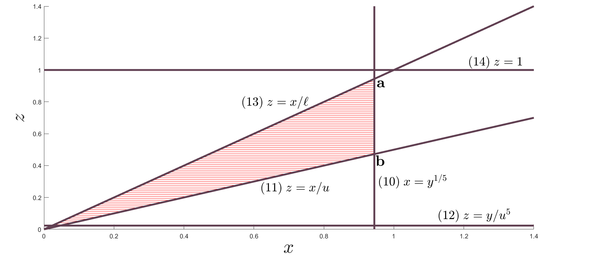
Figure 1: $f(x)=x^{5}$, $\ell=1$, $u=2$, $y=0.75\leq\ell^{5}=f(\ell)$

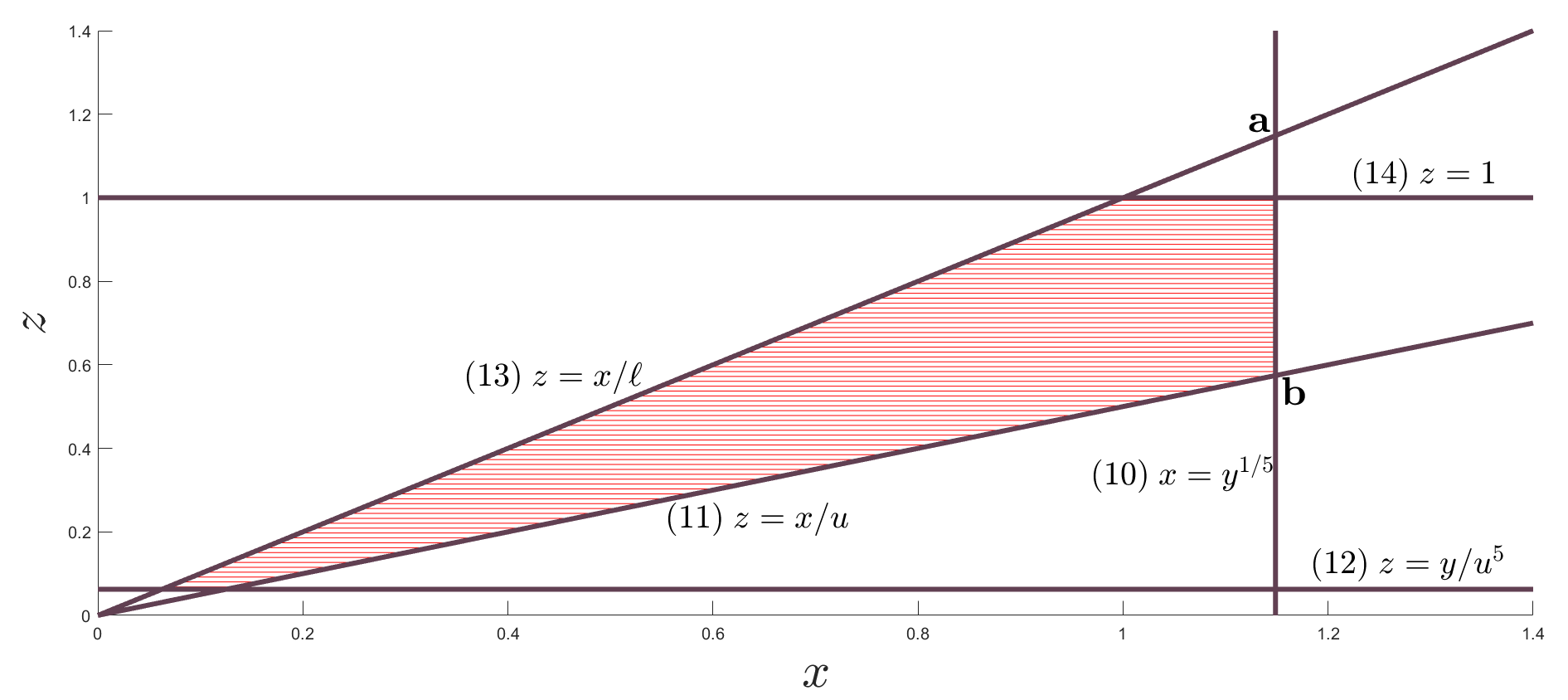
Figure 2: $f(x)=x^{5}$, $\ell=1$, $u=2$, $y=2>\ell^{5}=f(\ell)$

To understand why these two cases suffice, observe that together (11) and (13) create a ‘wedge’ in the positive orthant. $R_{y}$ is composed of this wedge intersected with $\{(x,z)\in\mathbb{R}^{2}:x\leq f^{-1}(y)\}$, for $\frac{y}{f(u)}\leq z\leq 1$. With a slight abuse of notation, based on context we use $(k)$, for $k=10,11,\dots,14$, to refer both to the inequality defined above and to the 1-d boundary of the region it describes.

Now consider the triangle formed by these ‘wedge’ inequalities, and the inequality $x\leq f^{-1}(y)$. The vertices of this triangle are $(0,0)$, $\mathbf{a}=(x_{a},z_{a}):=(f^{-1}(y),\frac{f^{-1}(y)}{\ell})$, and $\mathbf{b}=(x_{b},z_{b}):=(f^{-1}(y),\frac{f^{-1}(y)}{u})$. To understand the area that we are seeking to compute, we need to ascertain where $(0,0)$, $\mathbf{a}$, and $\mathbf{b}$ fall relative to (12) and (14), which bound the region $\frac{y}{f(u)}\leq z\leq 1$. Note that the origin falls on or below (12), and because $u>\ell$, $\mathbf{a}$ is always above $\mathbf{b}$ (in the sense of higher value of $z$).

We show that $\mathbf{b}$ must fall between the two lines (12) and (14). We know $y\leq f(u)$, which implies $f^{-1}(y)\leq u$ because $f$ is increasing. Therefore $\frac{f^{-1}(y)}{u}=z_{b}\leq 1$. Furthermore, because $f$ is continuous, convex, and increasing, by Lemma 1 we can see that $z_{b}=\frac{f^{-1}(y)}{u}\geq\frac{y}{f(u)}$.

Furthermore, given that $\mathbf{a}$ must be above $\mathbf{b}$, we now have our two cases: $\mathbf{a}$ is either above (14) (if $y>f(\ell)$), or on or below (14) (if $y\leq f(\ell)$).

Using the observations made above, we can now calculate the area of $R_{y}$ via integration. We integrate over $z$, and the limits of integration depend on the value of $y$. If $y\leq f(\ell)$, then the area is given by the expression:

$$\int_{\frac{y}{f(u)}}^{\frac{f^{-1}(y)}{u}}\left(uz-\ell z\right)\;dz+\int_{\frac{f^{-1}(y)}{u}}^{\frac{f^{-1}(y)}{\ell}}\left(f^{-1}(y)-\ell z\right)\;dz$$

If $y\geq f(\ell)$, then the area is given by the expression:

$$\int_{\frac{y}{f(u)}}^{\frac{f^{-1}(y)}{u}}\left(uz-\ell z\right)\;dz+\int_{\frac{f^{-1}(y)}{u}}^{1}\left(f^{-1}(y)-\ell z\right)\;dz$$

Note that when $y=f(\ell)$, these quantities are equal.

Integrating over $y$, we compute the volume of $\bar{S}^{0}_{f}(\ell,u)$ as follows:

$$\operatorname{vol}(\bar{S}^{0}_{f}(\ell,u))= \int_{0}^{f(\ell)}\left(\int_{\frac{y}{f(u)}}^{\frac{f^{-1}(y)}{u}}\left(uz-\ell z\right)\;dz+\int_{\frac{f^{-1}(y)}{u}}^{\frac{f^{-1}(y)}{\ell}}\left(f^{-1}(y)-\ell z\right)\;dz\right)\;dy$$

$$+\int_{f(\ell)}^{f(u)}\left(\int_{\frac{y}{f(u)}}^{\frac{f^{-1}(y)}{u}}\left(uz-\ell z\right)\;dz+\int_{\frac{f^{-1}(y)}{u}}^{1}\left(f^{-1}(y)-\ell z\right)\;dz\;\right)dy.$$

∎

The following corollary immediately follows from Theorem 3.2 and Lemma 1.

Corollary 3.

Suppose that $f$ is continuous, convex, and increasing on $[0,u]$, with $u>\ell>0$ and $f(0)=0$. Then

$$\operatorname{vol}(\invbreve{S}^{0}_{f}(\ell,u))= \operatorname{vol}(\bar{S}^{0}_{f}(\ell,u))-\operatorname{vol}(\Delta_{f}(\ell,u))$$

$$=\int_{0}^{f(\ell)}\left(\int_{\frac{y}{f(u)}}^{\frac{f^{-1}(y)}{u}}\left(uz-\ell z\right)\;dz+\int_{\frac{f^{-1}(y)}{u}}^{\frac{f^{-1}(y)}{\ell}}\left(f^{-1}(y)-\ell z\right)\;dz\right)\;dy$$

$$\quad+\int_{f(\ell)}^{f(u)}\left(\int_{\frac{y}{f(u)}}^{\frac{f^{-1}(y)}{u}}\left(uz-\ell z\right)\;dz+\int_{\frac{f^{-1}(y)}{u}}^{1}\left(f^{-1}(y)-\ell z\right)\;dz\;\right)dy$$

$$\quad-\frac{1}{6}(f(u)-f(\ell))(u-\ell).$$

In the following corollary, we consider a particular example of the exponential function first considered in Section 2.

Corollary 4.

Let $f(x):=b^{x}-1$, for $b>1$, with $u>\ell>0$. Then

$$\operatorname{vol}(\invbreve{S}^{0}_{f}(\ell,u)) =\frac{1}{6}(u-\ell)(b^{u}+b^{\ell}+1)-\frac{1}{(\ln b)^{2}}\left(\frac{b^{u}-1}{u}-\frac{b^{\ell}-1}{\ell}\right).$$

Putting this together with Corollary 2, we obtain:

Corollary 5.

Let $f(x):=b^{x}-1$, for $b>1$, with $u>\ell>0$. Then

$$\operatorname{vol}(\invbreve{S}^{0}_{f}(\ell,u))-\operatorname{vol}(\invbreve{S}^{*}_{f}(\ell,u))\\ =\frac{1}{6}(u-\ell)+\frac{1}{3\ln b}(b^{u}-b^{\ell})-\frac{1}{(\ln b)^{2}}\left(\frac{b^{u}-1}{u}-\frac{b^{\ell}-1}{\ell}\right).$$

If we fix $b>1$, and let $\ell=ku$ for some fixed $k\in(0,1)$, then

$$\lim_{u\to\infty}u\times\frac{\operatorname{vol}(\invbreve{S}^{0}_{f}(\ell,u))-\operatorname{vol}(\invbreve{S}^{*}_{f}(\ell,u))}{\operatorname{vol}(\invbreve{S}^{0}_{f}(\ell,u))}=\frac{2}{\ln b}.$$

Asymptotically, with respect to $u$, the fraction of the volume of the naïve relaxation that is “extra” beyond the perspective relaxation tends to 0 rather quickly as $u$ tends to $\infty$. What we can see, in this asymptotic regime, is that the naïve relaxation is not so bad, compared to the perspective relaxation.

3.2 $f(\ell)>0$.

So far, for the naïve relaxation, we have assumed that $f$ is defined on all of $[0,u]$ and that $f(0)=0$. Next, we extend the naïve relaxation and accompanying volume results to the case in which the domain of the given $f$ is considered to be restricted to $[\ell,u]$, with $u>\ell>0$. We wish to emphasize that the extension is relevant even when $f$ is naturally defined at 0 and has $f(0)=0$ (e.g., $f(x)=x^{p}$, $p>1$). Our strategy is to define the tightest convex under-estimator $g$ of $f$ that can be extended to pass through the origin, and then apply the naïve relaxation to $g$. This $g$ is the convex envelope (on $[0,u]$) of the function that is $0$ at $0$ and $f(x)$ on $[\ell,u]$. This strategy, including our choice of $g$, is quite natural, and is relevant to modelers facing this scenario.

Recall that for real (univariate) functions, convexity implies right differentiability. For the following lemma, we use the notation $\partial_{+}f(x)$ to indicate the right derivative of $f$ at $x$.

Lemma 6.

Let $f$ be positive, continuous, and convex on $[\ell,u]$ with with $u>\ell>0$, and let $a:=\max\{\hat{x}\in[\ell,u]:f(\hat{x})\leq\hat{x}\partial_{+}f(x),\mbox{ for all }x\in[\hat{x},u)\}$. Then

$$g(x):=\begin{cases}\frac{f(a)}{a}x,&\text{if }0\leq x\leq a;\\ f(x),&\text{if }a<x\leq u,\end{cases}$$

is the convex envelope (on $[0,u]$) of the function that is $0$ at $0$ and $f(x)$ on $[\ell,u]$. Moreover, $g$ is increasing (and thus invertible) on $[0,u]$.

Proof.

The linear part of $g$ (defined on $[0,a]$) has the maximum possible slope to both maintain convexity (and continuity) and pass through the origin. The slope of the linear part of $g$, $f(a)/a$, is positive because $0<\ell\leq a$ and $f$ is positive on $[\ell,u]$. This fact, along with the convexity of $g$, implies that $g$ is increasing on $[0,u]$. ∎

For a function $f$ that is continuous, positive, and convex on $[\ell,u]$, and is undefined or positive at 0, we define the naïve relaxation of $\invbreve{D}_{f}(\ell,u)$ to be $\invbreve{S}^{0}_{g}(\ell,u)$, where $g$ is defined relative to $f$ as in Lemma 6. Volume results for $\invbreve{S}^{0}_{g}(\ell,u)$ are provided in Theorem 3.7.

Theorem 3.7.

Let $f$ be positive, continuous, and convex on $[\ell,u]$, with $u>\ell>0$, and define $g$ as in Lemma 6. Then $\invbreve{D}_{f}(\ell,u)\subseteq\invbreve{S}^{0}_{g}(\ell,u)$, and

$$\operatorname{vol}(\invbreve{S}^{0}_{g}(\ell,u))=\operatorname{vol}(\bar{S}^{0}_{g}(\ell,u))-\frac{1}{6}(f(u)-f(\ell))(u-\ell),$$

where $\operatorname{vol}(\bar{S}^{0}_{g}(\ell,u))$ is computed as follows.

If $a:=\ell$, then

$$\operatorname{vol}(\bar{S}^{0}_{g}(\ell,u)= \int_{0}^{f(\ell)}\left(\int_{\frac{y}{f(u)}}^{\frac{y\ell}{f(\ell)u}}\left(uz-\ell z\right)\;dz+\int_{\frac{y\ell}{f(\ell)u}}^{\frac{y}{f(\ell)}}\left(\frac{y\ell}{f(\ell)}-\ell z\right)\;dz\right)\;dy$$

$$+\int_{f(\ell)}^{f(u)}\left(\int_{\frac{y}{f(u)}}^{\frac{g^{-1}(y)}{u}}\left(uz-\ell z\right)\;dz+\int_{\frac{g^{-1}(y)}{u}}^{1}\left(g^{-1}(y)-\ell z\right)\;dz\;\right)dy.$$

If $a\in(\ell,u)$, then

$$\operatorname{vol}(\bar{S}^{0}_{f}(\ell,u))= \int_{0}^{\frac{f(a)\ell}{a}}\left(\int_{\frac{y}{f(u)}}^{\frac{ya}{f(a)u}}\left(uz-\ell z\right)\;dz+\int_{\frac{ya}{f(a)u}}^{\frac{ya}{f(a)\ell}}\left(\frac{ya}{f(a)}-\ell z\right)\;dz\right)\;dy$$

$$+\int_{\frac{f(a)\ell}{a}}^{f(a)}\left(\int_{\frac{y}{f(u)}}^{\frac{ya}{f(a)u}}\left(uz-\ell z\right)\;dz+\int_{\frac{ya}{f(a)u}}^{1}\left(\frac{ya}{f(a)}-\ell z\right)\;dz\;\right)dy$$

$$+\int_{f(a)}^{f(u)}\left(\int_{\frac{y}{f(u)}}^{\frac{g^{-1}(y)}{u}}\left(uz-\ell z\right)\;dz+\int_{\frac{g^{-1}(y)}{u}}^{\ell}\left(g^{-1}(y)-\ell z\right)\;dz\;\right)dy.$$

If $a:=u$, then

$$\operatorname{vol}(\bar{S}^{0}_{f}(\ell,u))= \int_{0}^{\frac{f(u)\ell}{u}}\left(\int_{\frac{y}{f(u)}}^{\frac{yu}{f(u)\ell}}\left(\frac{yu}{f(u)}-\ell z\right)\;dz\right)\;dy$$

$$+\int_{\frac{f(u)\ell}{u}}^{f(u)}\left(\int_{\frac{y}{f(u)}}^{\ell}\left(\frac{yu}{f(u)}-\ell z\right)\;dz\;\right)dy.$$

Proof.

Apply Corollary 3 to $g$, and then use Lemma 1. ∎

In the context of convex-optimization solvers, instantiating the model $\invbreve{S}^{0}_{g}(\ell,u)$ generally requires special handling for piecewise functions; this can be addressed via coding of $g$ (function values and derivatives) for use by NLP solvers, or through a feature of SCIP that can accomodate piecewise-defined convex increasing functions through the modeling language AMPL (see comments about this feature of SCIP in XuLeeSkipper2019 and in Section 6.2 of LeeSkipper2017 ).

Next, we apply Theorem 3.7 to $f(x):=x^{p}$ as a third alternative to the naïve and the perspective relaxations. Per Lemma 6, we have,

$$g(x):=\begin{cases}\ell^{p-1}x,&\text{if }0\leq x\leq\ell;\\ x^{p},&\text{if }\ell<x\leq u.\end{cases}$$

In this case, because $f(x)$ is convex on $[0,\ell]$ with $f(0)=0$, the linear part of $g$ provides an upper bound on $f$ over $[0,\ell]$. Furthermore, because $g(x)$ is the point-wise maximum of $f(x)$ and $\frac{f(\ell)}{\ell}x$, we can efficiently realize $\invbreve{S}^{0}_{g}(\ell,u)$ simply by appending $y\geq\frac{f(\ell)}{\ell}x$ to $\invbreve{S}^{0}_{f}(\ell,u)$. We have

$$\invbreve{S}^{*}_{f}(\ell,u)\subset\invbreve{S}^{0}_{g}(\ell,u)\subset\invbreve{S}^{0}_{f}(\ell,u).$$

We are interested in comparing the quality of relaxation the piecewise method provides compared to the perspective relaxation, so we compare the difference of each relative to the naïve relaxation.

Corollary 8.

Let $f(x):=x^{p}$, for $x\in[0,u]$, with $u>\ell>0$, and let $g$ be defined per Lemma 6. Then

$$\frac{\invbreve{S}^{0}_{f}(\ell,u)-\invbreve{S}^{0}_{g}(\ell,u)}{\invbreve{S}^{0}_{f}(\ell,u)-\invbreve{S}^{*}_{f}(\ell,u)} ~{}=~{}(p+1)\frac{1-\left(\frac{\ell}{u}\right)}{\left(\frac{u}{\ell}\right)^{p+1}-1}.$$

Proof.

Follows directly from Theorem 2.1, Corollary 3, and Theorem 3.7. ∎

Next, we will see that for power functions, when $\ell$ is big enough relative to $u$, much of what can be achieved by the perspective relaxation (relative to the naïve relaxation) can already be achieved by the naïve relaxation applied to the piecewise function $g$ of Lemma 6.

Corollary 9.

Let $f(x):=x^{p}$, for $x\in[0,u]$, with $u>\ell>0$, and let $g$ be defined per Lemma 6. Then for each $p>1$ and $\phi\in(0,1)$, there is a $k(p,\phi)\in(0,1)$, so that $\ell/u$ > $k(p,\phi)$, if and only if

$$\frac{\invbreve{S}^{0}_{f}(\ell,u)-\invbreve{S}^{0}_{g}(\ell,u)}{\invbreve{S}^{0}_{f}(\ell,u)-\invbreve{S}^{*}_{f}(\ell,u)} >\phi.$$

Proof.

Let

$$\phi:=(p+1)\frac{1-k}{1/k^{p+1}-1}.$$

First, we note that $\lim_{k\rightarrow 1^{-}}~{}\phi=1$. So, we only need to check that the continuous function $\phi$ is increasing in $k$ on $(0,1)$.

We compute

$$\frac{d\phi}{dk}=\frac{k^{p}(1+p)(1+k^{2+p}+p-k(2+p))}{(1-k^{1+p})^{2}}.$$

To see that this is positive, we only need to consider the factor

$$j:=1+k^{2+p}+p-k(2+p).$$

For each $p$, it is clear that $j$ is continuous over $k\in(0,1)$. The limit of $j$, as $k\rightarrow 0$ is $p+1$, and the limit of $j$, as $k\rightarrow 1$ is $0$. So, extending the definition of $j$ to all $k\in[0,1]$, we have now a continuous function on $[0,1]$, starting at value $p+1$ and ending at value $0$. Now

$$\frac{dj}{dk}=-2-p+k^{1+p}(2+p)=(k^{1+p}-1)(2+p),$$

which is negative for all $k\in(0,1)$. Therefore $j$ is decreasing on $(0,1)$. Because $j$ starts at a positive value ($p+1$), and decreases all the way to 0, it is positive on all of $(0,1)$. Therefore, $\frac{d\phi}{dk}>0$ on $(0,1)$, and so $\phi$ is increasing in $k$.

∎

Note that because of Corollary 9 and its proof, it is easy to compute $k(p,\phi)$ to any desired accuracy by a univariate search method (e.g., golden-section search).

4 Convex power functions

In this section we focus on the special case of $f(x):=x^{p}$, for $p>1$. For these convex power functions, we are able to obtain not only the perspective relaxation and the naïve relaxation, but a nested family of relaxations, “interpolating” between the perspective relaxation and the naïve relaxation.

For real scalars $u>\ell>0$ and $p>1$, we define

$$S_{p}(\ell,u):=\left\{(x,y,z)\in\mathbb{R}^{2}\times\{0,1\}~{}:~{}y\geq x^{p},~{}uz\geq x\geq\ell z\right\},$$

and, for $0\leq q\leq p-1$, the associated relaxations

$$S^{q}_{p}(\ell,u):=\left\{(x,y,z)\in\mathbb{R}^{3}~{}:~{}yz^{q}\geq x^{p},~{}uz\geq x\geq\ell z,~{}1\geq z\geq 0,~{}y\geq 0\right\}.$$

For $q=p-1$, we have the perspective relaxation; that is, $S^{p-1}_{p}(\ell,u)=S^{*}_{f}(\ell,u)$, for $f(x):=x^{p}$. Furthermore, if we define $0^{0}=1$, then for $q=0$, we have the naïve relaxation; that is, $S^{0}_{p}(\ell,u)=S^{0}_{f}(\ell,u)$, for $f(x):=x^{p}$.

Note that even though $x^{p}-yz^{q}$ is not a convex function for $q>0$ (even for $p=2,q=1$), the set $S^{q}_{p}(\ell,u)$ is convex. In fact, the set $S^{q}_{p}(\ell,u)$ is higher-dimensional-power-cone representable, which makes working with it appealing. The higher-dimensional power cone is defined as

$$\mathcal{K}_{{\bm{\alpha}}}^{(n)}:=\left\{(x,z)\in\mathbb{R}^{n}_{+}\times\mathbb{R}~{}:~{}\textstyle\prod_{j=1}^{n}x_{j}^{\alpha_{j}}\geq|z|\right\},$$

where ${\bm{\alpha}}\in\mathbb{R}^{n}_{+}$, $\mathbf{e}^{\prime}{\bm{\alpha}}=1$; see (Chares, , Sec. 4.1.2) and (cookbook, , Chap. 4), for example. It is easy to check that with $x,y,z\geq 0$, we have that $yz^{q}\geq x^{p}$ is equivalent, under the linear equation $u=1$, to $y^{\frac{1}{p}}z^{\frac{q}{p}}u^{1-\frac{q+1}{p}}\geq x$, which is in the format of the higher-dimensional power cone, when $q\in[1,p-1]$.

Still, computationally handling higher-dimensional power cones efficiently is not a trivial matter, and we should not take it on without considering alternatives.

As they are defined, both $S_{p}(\ell,u)$ and $S^{q}_{p}(\ell,u)$ are unbounded in the increasing $y$ direction. However, as before, we can add a simple linear inequality to ensure that our sets are bounded. We have

$$\bar{S}^{q}_{p}(\ell,u):=\left\{(x,y,z)\in\mathbb{R}^{3}~{}:~{}zu^{p}\geq y,~{}yz^{q}\geq x^{p},~{}uz\geq x\geq\ell z,~{}1\geq z\geq 0\right\}.$$

Ultimately, we are interested in the stronger upper bound on $y$ bound, yielding the set

$$\invbreve{S}^{q}_{p}(\ell,u):=\Big{\{}(x,y,z)\in\mathbb{R}^{3}~{}:~{} \left(\ell^{p}-\frac{u^{p}-\ell^{p}}{u-\ell}\ell\right)z+\frac{u^{p}-\ell^{p}}{u-\ell}x\geq y,$$

$$~{}yz^{q}\geq x^{p},~{}uz\geq x\geq\ell z,~{}1\geq z\geq 0\Big{\}}.$$

However, as we have seen, computing the volume is easier with the simpler bound on $y$. We can then use Lemma 1 to easily obtain the volume of $\invbreve{S}^{q}_{p}(\ell,u)$.

The following result, part of which is closely related to results in Akturk , is easy to establish.

Proposition 1.

For $u>\ell>0$, $p>1$, and $q\in[0,p-1]$, (i) $\bar{S}_{p}(\ell,u)\subseteq\bar{S}_{p}^{q}(\ell,u)$ , (ii) $\bar{S}_{p}^{q}(\ell,u)$ is a convex set, (iii) $\bar{S}_{p}^{q}(\ell,u)\subseteq\bar{S}_{p}^{q^{\prime}}(\ell,u)$, for $0\leq q^{\prime}\leq q$, and (iv) $\operatorname{conv}(\bar{S_{p}(\ell,u)})=\bar{S}_{p}^{p-1}(\ell,u)$ .

Proof.

(i): For $(\hat{x},\hat{y},\hat{z})\in\bar{S}_{p}(\ell,u)$, it is easy to check that $(\hat{x},\hat{y},\hat{z})\in\bar{S}_{p}^{q}(\ell,u)$, considering the two cases: $\hat{z}=0$ and $\hat{z}=1$. (ii): For $q\in[0,p-1]$, $\bar{S}_{p}^{q}(\ell,u)$ is an affine slice of a higher-dimensional power cone. (iii): Because $y\geq 0$, we have that $yz^{q}$ is non-increasing in $q$ for all $z\in[0,1]$. (iv): By (i), we have $\bar{S}_{p}(\ell,u)\subseteq\bar{S}_{p}^{p-1}(\ell,u)$. By (ii), we have that $\bar{S}_{p}^{p-1}(\ell,u)$ is a convex set. Therefore, $\operatorname{conv}(\bar{S_{p}}(\ell,u))\subseteq\bar{S}_{p}^{p-1}(\ell,u)$ . For the reverse inclusion, consider $\hat{\xi}:=(\hat{x},\hat{y},\hat{z})\in\bar{S}_{p}^{p-1}(\ell,u)$. If $\hat{z}=0$, then $\hat{\xi}=(0,0,0)\in\bar{S}_{p}(\ell,u)\subseteq\operatorname{conv}(\bar{S}_{p}(\ell,u))$. If instead $0<\hat{z}\leq 1$, let $\hat{\xi}^{1}:=(\frac{\hat{x}}{\hat{z}},\frac{\hat{y}}{\hat{z}},1)$. A quick check verifies that $\hat{\xi}^{1}\in\bar{S}_{p}(\ell,u)$ (in particular, $\left(\frac{\hat{y}}{\hat{z}}\right)\geq\left(\frac{\hat{x}}{\hat{z}}\right)^{p}$ because $\hat{y}\hat{z}^{p-1}\geq\hat{x}^{p}$). So we have that $\hat{\xi}~{}=~{}(1-\hat{z})(0,0,0)+\hat{z}\hat{\xi}^{1}~{}\in~{}\operatorname{conv}(\bar{S}_{p}(\ell,u))$. ∎

Note that when $q=0$, we can set $f(x):=x^{p}$ and use the formula obtained in Theorem 3.2 to obtain the volume of $\operatorname{vol}(\bar{S}_{p}^{0}(\ell,u))$.

Corollary 2.

For $p>1$, and $u>\ell>0$,

$$\operatorname{vol}(\bar{S}_{p}^{0}(\ell,u))=\frac{\left(p^{2}+3p-1\right)u^{p+1}+3{\ell}^{p+1}-\left(p^{2}+3p+2\right){\ell}u^{p}}{3(p+1)(p+2)}.$$

Extending Corollary 2, we have the following result.

Theorem 4.3.

For $p>1$, $0\leq q\leq p-1$, and $u>\ell>0$,

$$\operatorname{vol}(\bar{S}_{p}^{q}(\ell,u))=\frac{(p^{2}-pq+3p-q-1)u^{p+1}+3\ell^{p+1}-(p+1)(p-q+2)\ell u^{p}}{3(p+1)(p-q+2)}.$$

Proof.

The case of $q=0$ is Corollary 2, so we can assume that $q>0$. The proof structure of Theorem 4.3 is similar to that of Theorem 3.2, therefore, once again we proceed using standard integration techniques. We fix the variable $y$ and consider the corresponding 2-dimensional slice, $R_{y}$, of $\bar{S}_{p}^{q}(\ell,u)$. In the $(x,z)$-space, $R_{y}$ is described by:

$$z \geq x^{p/q}y^{-1/q}$$ (16)

$$z \geq x/u$$ (17)

$$z \geq y/u^{p}$$ (18)

$$z \leq x/\ell$$ (19)

$$z \leq 1$$ (20)

$$z \geq 0$$ (21)

These inequalities are those in Theorem 3.2 with the exception of (16), and, analogous to the proof of Theorem 3.2, the tight inequalities for $R_{y}$ are among (16), (17), (18), (19), and (20) for all choices of $p$, $q$, $\ell$, $u$, and $y$. Furthermore, the region will always be described by either the entire set of inequalities (if $y>\ell^{p}$), or (16), (17), (18), and (19) (if $y\leq\ell^{p}$). For an illustration of these two cases with $p=5$ and $q=3$, see Figures 3, 4.

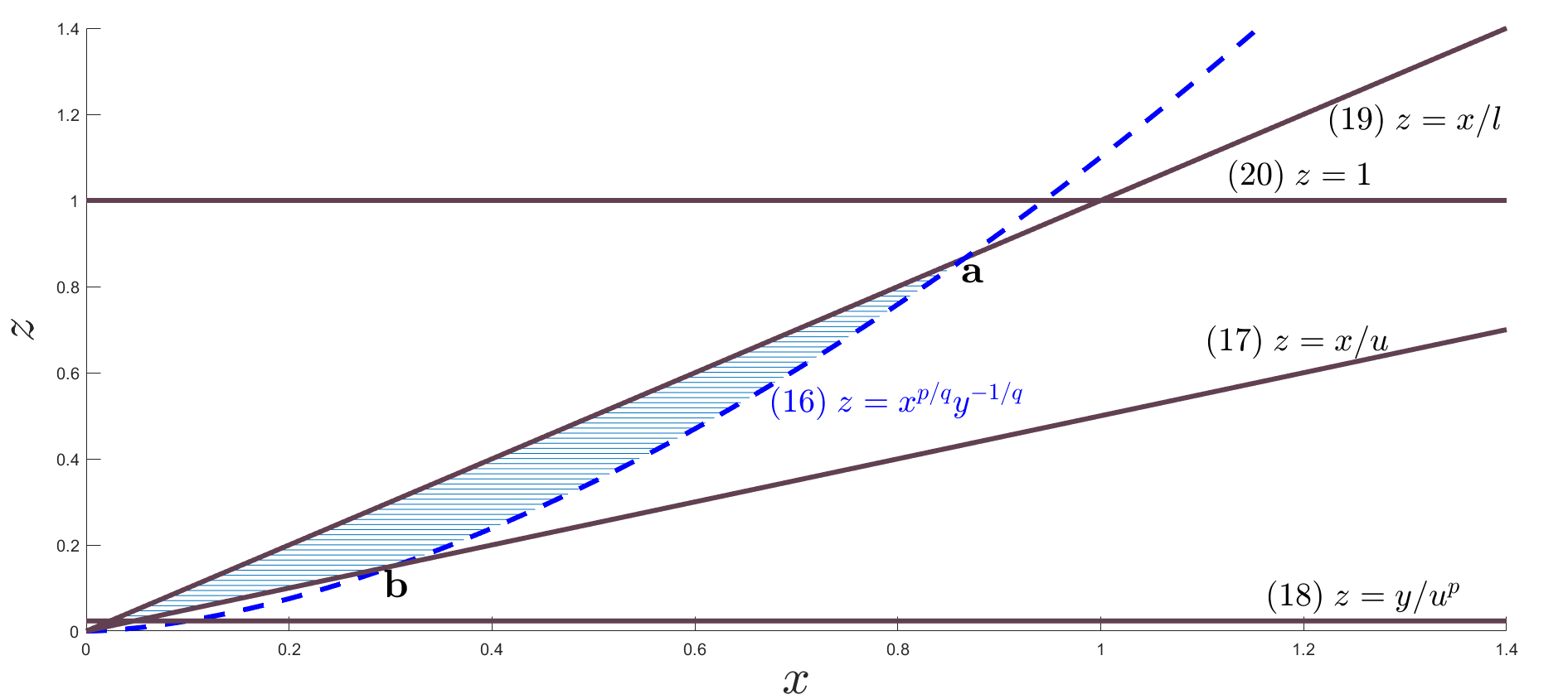
Figure 3: $p=5$, $q=3$, $\ell=1$, $u=2$, $y=0.75\leq\ell^{p}$

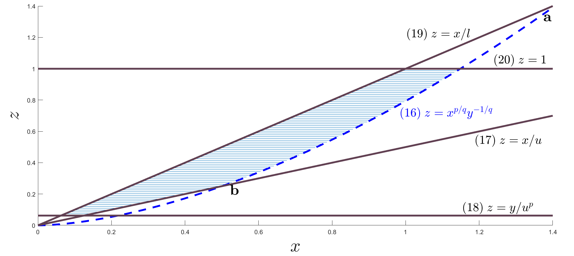
Figure 4: $p=5$, $q=3$, $\ell=1$, $u=2$, $y=2>\ell^{p}$

To understand why these two cases suffice, recall that together (17) and (19) create a ‘wedge’ in the positive orthant. $R_{y}$ is composed of this wedge intersected with $\{(x,z)\in\mathbb{R}^{2}:z\geq x^{p/q}y^{-1/q}\}$, for $\frac{y}{u^{p}}\leq z\leq 1$. As before, we slightly abuse notation and based on context we use $(k)$, for $k=16,17,\dots,20$, to refer both to the inequality defined above and to the 1-d boundary of the region it describes.

We consider the set of points formed by the wedge and the inequality $z\geq x^{p/q}y^{-1/q}$. Curves (16) and (19) intersect at $(0,0)$ and $\mathbf{a}=(x_{a},z_{a}):=\left(\left(\frac{y}{\ell^{q}}\right)^{1/(p-q)},\right.$ $\left.\left(\frac{y}{\ell^{p}}\right)^{1/(p-q)}\right)$. Curves (16) and (17) intersect at $(0,0)$ and $\mathbf{b}=(x_{b},z_{b}):=\left(\left(\frac{y}{u^{q}}\right)^{1/(p-q)},\right.$ $\left.\left(\frac{y}{u^{p}}\right)^{1/(p-q)}\right)$. As before, to understand the area that we are seeking to compute, we need to ascertain where $(0,0)$, $\mathbf{a}$, and $\mathbf{b}$ fall relative to (18) and (20), which bound the region $\frac{y}{u^{p}}\leq z\leq 1$. Note that the origin falls on or below (18), and because $u>\ell$, $\mathbf{a}$ is always above $\mathbf{b}$ (in the sense of higher value of $z$).

We show that $\mathbf{b}$ must fall between lines (18) and (20). This is equivalent to $\frac{y}{u^{p}}\leq\left(\frac{y}{u^{p}}\right)^{1/(p-q)}=z_{b}\leq 1$. Now, we know $y\leq u^{p}$, which implies $\frac{y}{u^{p}}\leq 1$. From our assumptions on $p$ and $q$, we also have $0<\frac{1}{p-q}\leq 1$. From this we can immediately conclude $\frac{y}{u^{p}}\leq\left(\frac{y}{u^{p}}\right)^{1/(p-q)}=z_{b}\leq 1$.

Furthermore, given that $\mathbf{a}$ must be above $\mathbf{b}$, we now have our two cases: $\mathbf{a}$ is either above (20) (if $y>\ell^{p}$), or on or below (20) (if $y\leq\ell^{p}$). Using the observations made above, we can now calculate the area of $R_{y}$ via integration. We integrate over $z$, and the limits of integration depend on the value of $y$. If $y\leq\ell^{p}$, then the area is given by the expression:

$$\int_{\frac{y}{u^{p}}}^{z_{b}}\left(uz-\ell z\right)\;dz+\int_{z_{b}}^{z_{a}}\left((yz^{q})^{\frac{1}{p}}-\ell z\right)\;dz.$$

If $y\geq\ell^{p}$, then the area is given by the expression:

$$\int_{\frac{y}{u^{p}}}^{z_{b}}\left(uz-\ell z\right)\;dz+\int_{z_{b}}^{1}\left((yz^{q})^{\frac{1}{p}}-\ell z\right)\;dz.$$

Note that when $y=\ell^{p}$, these quantities are equal. Furthermore, when $q=p-1$ (and we have the hull), the first integral in each sum is equal to zero.

Integrating over $y$, we compute the volume of $\bar{S}_{p}^{q}(\ell,u)$ as follows:

$$\int_{0}^{\ell^{p}}\left(\int_{\frac{y}{u^{p}}}^{\left(\frac{y}{u^{p}}\right)^{1/(p-q)}}\left(uz-\ell z\right)\;dz+\int_{\left(\frac{y}{u^{p}}\right)^{1/(p-q)}}^{\left(\frac{y}{l^{p}}\right)^{1/(p-q)}}\left((yz^{q})^{\frac{1}{p}}-\ell z\right)\;dz\right)\;dy$$

$$+\int_{\ell^{p}}^{u^{p}}\left(\int_{\frac{y}{u^{p}}}^{\left(\frac{y}{u^{p}}\right)^{1/(p-q)}}\left(uz-\ell z\right)\;dz+\int_{\left(\frac{y}{u^{p}}\right)^{1/(p-q)}}^{1}\left((yz^{q})^{\frac{1}{p}}-\ell z\right)\;dz\;\right)dy$$

$$=\frac{(p^{2}-pq+3p-q-1)u^{p+1}+3\ell^{p+1}-(p+1)(p-q+2)\ell u^{p}}{3(p+1)(p-q+2)}.$$

∎

By looking at these slices in the $(x,z)$ plane, we are able to gain a better geometric understanding of how the relaxation is tightening as $q$ increases from $0$ to $p-1$. See Figure 5 to see how the relaxation improves as $q$ increases. The figure is drawn for the case where $y\geq\ell^{p}$ but the picture would be very similar for the alternative case. When $q=p-1$ (and we have precisely the convex hull), inequality (11) becomes redundant; this is equivalent to when we noted in the proof that the first integral is equal to zero when we have the hull.

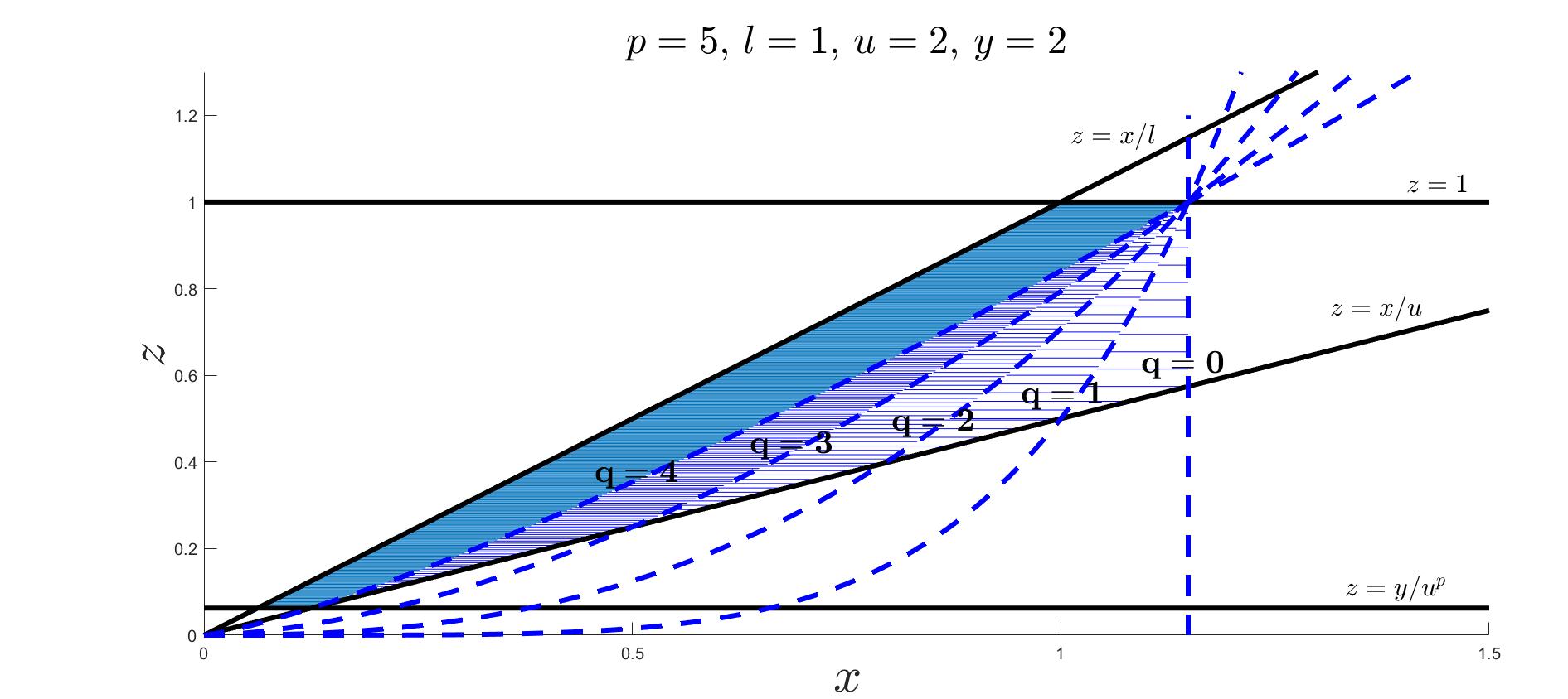
Figure 5: Increasing $q$ tightens the relaxation.

Now the following corollary follows from Theorem 4.3 (and its proof) and (the proof of) Lemma 1.

Corollary 4.

For $p>1$, $0\leq q\leq p-1$, , and $u>\ell>0$,

$$\operatorname{vol}(\invbreve{S}_{p}^{q}(\ell,u))=$$

$$\frac{(p^{2}-pq+3p-q-1)u^{p+1}+3\ell^{p+1}-(p+1)(p-q+2)\ell u^{p}}{3(p+1)(p-q+2)}-\frac{(u^{p}-\ell^{p})(u-\ell)}{6}.$$

Note that for $q=p-1$, this is exactly what we get by plugging $f(x)=x^{p}$ into Theorem 2.1.

We can use the volume formula of Corollary 4 to compare relaxations. For the most general case, we have the following.

Corollary 5.

For $p>1$, $0\leq q_{1}<q_{2}\leq p-1$, and $u>\ell>0$,

$$\operatorname{vol}(\invbreve{S}_{p}^{q_{1}}(\ell,u))-\operatorname{vol}(\invbreve{S}_{p}^{q_{2}}(\ell,u))=\frac{(q_{2}-q_{1})(u^{p+1}-\ell^{p+1})}{(p+1)(p-q_{1}+2)(p-q_{2}+2)}.$$

Applying this result, we can precisely quantify how much better the perspective relaxation ($q=p-1$) is compared to the naïve relaxation ($q=0$):

Corollary 6.

For $p>1$, and $u>\ell>0$,

$$\operatorname{vol}(\invbreve{S}_{p}^{0}(\ell,u))-\operatorname{vol}(\invbreve{S}_{p}^{p-1}(\ell,u))=\frac{(p-1)(u^{p+1}-\ell^{p+1})}{3(p+1)(p+2)}\quad\left[=\frac{u^{3}-\ell^{3}}{36},\mbox{ for }p=2\right].$$

It is also interesting to quantify how much better the perspective relaxation ($q=p-1$) is compared to the “naïve perspective relaxation” ($q=1$):

Corollary 7.

For $p>2$, and $u>\ell>0$,

$$\operatorname{vol}(\invbreve{S}_{p}^{1}(\ell,u))-\operatorname{vol}(\invbreve{S}_{p}^{p-1}(\ell,u))=\frac{(p-2)(u^{p+1}-\ell^{p+1})}{3(p+1)^{2}}.$$

To see if a tighter relaxation is worth the extra computational effort, it is useful to see what proportion of the volume is removed when replacing a weaker relaxation to a stronger one. Our volume formula leads to a lower bound, in terms of $p$, $q_{1}$ and $q_{2}$, on the proportion of the excess volume removed when replacing $\invbreve{S}_{p}^{q_{1}}(\ell,u)$ by $\invbreve{S}_{p}^{q_{2}}(\ell,u)$, for $q_{1}<q_{2}$. Interestingly:

• The exact formula only depends on $\ell$ and $u$ through their ratio $k$.

• We have a lower bound that is completely independent of $\ell$ and $u$.

Corollary 8.

For $p>1$, $0\leq q_{1}<q_{2}\leq p-1$, $u>\ell>0$, and $k:=\ell/u$,

$$\frac{\operatorname{vol}(\invbreve{S}_{p}^{q_{1}}(\ell,u))-\operatorname{vol}(\invbreve{S}_{p}^{q_{2}}(\ell,u))}{\operatorname{vol}(\invbreve{S}_{p}^{q_{1}}(\ell,u))}$$

$$\quad=\frac{6(q_{2}-q_{1})\left(\frac{1-k^{p+1}}{(1-k)(1+k^{p})}\right)}{(p-q_{2}+2)(p^{2}+3p-q_{1}(p+1)-1)-3(p-q_{2}+2)\left(\frac{(1+k)(1-k^{p})}{(1-k)(1+k^{p})}\right)}$$

$$\quad\geq\frac{6(q_{2}-q_{1})}{(p-q_{2}+2)(p^{2}+3p-q_{1}(p+1)-4)}.$$

Moreover, the inequality becomes tight only as $k\rightarrow 0$.

Proof.

Replacing $\ell$ with $ku$ and combining terms in the volume expression in Corollary 4, we see that $u$ arises only in a factor of $u^{p+1}$ of the entire volume expression:

$$\operatorname{vol}(\invbreve{S}_{p}^{q_{1}}(\ell,u))=\\ \frac{u^{p+1}\left[2(p^{2}+3p-pq_{1}-q_{1}-1)+6k^{p+1}-(p+1)(p-q_{1}+2)(k^{p+1}-k^{p}+k+1)\right]}{6(p+1)(p-q_{1}+2)}.$$

Similarly, replacing $\ell$ with $ku$ in the difference of volumes expression in Corollary 5, we obtain the same $u^{p+1}$ factor,

$$\operatorname{vol}(\invbreve{S}_{p}^{q_{1}}(\ell,u))-\operatorname{vol}(\invbreve{S}_{p}^{q_{2}}(\ell,u))=\frac{u^{p+1}(q_{2}-q_{1})(1-k^{p+1})}{(p+1)(p-q_{1}+2)(p-q_{2}+2)},$$

so that in the ratio, the $u$ factors cancel:

$$\frac{\operatorname{vol}(\invbreve{S}_{p}^{q_{1}}(\ell,u))-\operatorname{vol}(\invbreve{S}_{p}^{q_{2}}(\ell,u))}{\operatorname{vol}(\invbreve{S}_{p}^{q_{1}}(\ell,u))}=$$

$$\frac{6(q_{2}-q_{1})(1-k^{p+1})}{(p-q_{2}+2)\left[2(p^{2}-pq_{1}+3p-q_{1}-1)+6k^{p+1}-(p+1)(p-q_{1}+2)(k^{p+1}-k^{p}+k+1)\right]}.$$

Letting $A:=k^{p+1}-k^{p}+k+1$ and simplifying further, we obtain:

$$\frac{\operatorname{vol}(\invbreve{S}_{p}^{q_{1}}(\ell,u))-\operatorname{vol}(\invbreve{S}_{p}^{q_{2}}(\ell,u))}{\operatorname{vol}(\invbreve{S}_{p}^{q_{1}}(\ell,u))}$$

$$= \frac{6(q_{2}-q_{1})(1-k^{p+1})}{(p-q_{2}+2)\left[2(p^{2}-pq_{1}+3p-q_{1}-1)+(6k^{p+1}-Ap^{2}+Apq_{1}-3Ap+Aq_{1}-2A)\right]}$$

$$= \frac{6(q_{2}-q_{1})(1-k^{p+1})}{(p-q_{2}+2)\left[2(p^{2}-pq_{1}+3p-q_{1}-1)-A(p^{2}-pq_{1}+3p-q_{1}-1)-(3A-6k^{p+1})\right]}$$

$$= \frac{6(q_{2}-q_{1})(1-k^{p+1})}{(p-q_{2}+2)\left[(2-A)(p^{2}-pq_{1}+3p-q_{1}-1)-3(A-2k^{p+1})\right]}$$

$$= \frac{6(q_{2}-q_{1})\left(\frac{1-k^{p+1}}{2-A}\right)}{(p-q_{2}+2)(p^{2}-pq_{1}+3p-q_{1}-1)-3(p-q_{2}+2)\left(\frac{A-2k^{p+1}}{2-A}\right)},$$

which is the second expression in the statement of the corollary when $A$ is replaced by its equivalent expression.

Recalling that $0<k<1$ and $p>1$, it is clear that

$$2-A=(1-k)(1+k^{p})>0$$

and

$$2-A=(1-k^{p})-k(1-k^{p-1})\leq 1-k^{p},$$

so that

$$\frac{1-k^{p+1}}{2-A}\geq 1.$$

Similarly,

$$\frac{A-2k^{p+1}}{2-A}=\frac{(1-k^{p+1})+k(1-k^{p})}{(1-k^{p+1})-k(1-k^{p})}\geq 1,$$

and the lower bound follows. When the ratio of volumes is expressed in this form, it is clear that the bound is tight if $k=0$ and strict if $k>0$. ∎

Applying this result with $q_{1}=0$ and $q_{2}=p-1$ demonstrates that the excess volume of the naïve relaxation, as compared to the perspective relaxation, is substantial.

Corollary 9.

For $p>1$, $u>\ell>0$, and $k:=\ell/u$,

$$\frac{\operatorname{vol}(\invbreve{S}_{p}^{0}(\ell,u))-\operatorname{vol}(\invbreve{S}_{p}^{p-1}(\ell,u))}{\operatorname{vol}(\invbreve{S}_{p}^{0}(\ell,u))}=\frac{2(p-1)\left(\frac{1-k^{p+1}}{(1-k)(1+k^{p})}\right)}{(p^{2}+3p-1)-3\left(\frac{(1+k)(1-k^{p})}{(1-k)(1+k^{p})}\right)}\geq\frac{2}{p+4}~{}.$$

Moreover, the inequality becomes tight only as $k\rightarrow 0$.

5 Computational experiments

Some earlier theoretical results on using volume as a measure to compare relaxations were substantiated by computational experiments. Results in LM1994 concerning facility location were computationally substantiated in Lee2007 . Results in SpeakmanLee2015 concerning models for triple products were experimentally validated in SpeakmanYuLee .

In this section we describe some illustrative computations related to our present work. This is not meant to be a thorough computational study. Rather, we simply wish to illustrate what our theoretical results can predict about actual computational tradeoffs.

We carried out experiments on a 16-core machine (running Windows Server 2012 R2): two Intel Xeon CPU E5-2667 v4 processors running at 3.20GHz, with 8 cores each, and 128 GB of memory. We used the conic solver SDPT3 4.0 (sdpt3 ) under the Matlab “disciplined convex optimization” package CVX (cvx ).

5.1 Separable quadratic-cost knapsack covering.

Our first experiment is based on the following model, which we think of as a relaxation of the identical model having the constraints $z_{i}\in\{0,1\}$ for $i=1,2,\ldots,n$. The data $\mathbf{c},\mathbf{f},\mathbf{a},\mathbf{l},\mathbf{u}\in\mathbb{R}^{n}$ and $b\in\mathbb{R}$ are all positive. The idea is that we have costs $c_{i}$ on $x_{i}^{2}$, and $x_{i}$ is either 0 or in the “operating range” $[\ell_{i},u_{i}]$. We pay a cost $f_{i}$ when $x_{i}$ is nonzero.

$$\min\ \mathbf{c}^{\prime}\mathbf{y}+\mathbf{f}^{\prime}\mathbf{z}$$

subject to:

$$\mathbf{a}^{\prime}\mathbf{x}\geq b~{};$$

$$u_{i}z_{i}\geq x_{i}\geq\ell_{i}z_{i}~{},\qquad i=1,\ldots,n~{};$$

$$u_{i}^{2}z\geq y_{i}\geq x_{i}^{2}~{},\qquad i=1,\ldots,n~{};$$

$$1\geq z_{i}\geq 0,\qquad i=1,\ldots,n~{}.$$

In our experiment, we independently and randomly chose $a_{i}\sim\mathcal{U}(1.0,1.2)$, $f_{i}\sim\mathcal{U}(10.0,10.2)$, $\ell_{i}\sim\mathcal{U}(0,20)$, $\delta_{i}\sim\mathcal{U}(10,11)$, $u_{i}:=\ell_{i}+\delta_{i}$, $c_{i}\sim\mathcal{U}(0,1)$, $b:=\mathbf{a}^{\prime}(\bm{\ell}+\frac{1}{4}\bm{\delta})$. We purposely chose most of the parameters and the ranges $u_{i}-\ell_{i}=\delta_{i}$ to have very low variance, and we took $n=30,000$ so that we would get a strong averaging behavior. In this way, we sought to focus on the dependence of our results on the values of the $\ell_{i}$ and $u_{i}$, but not on the difference $u_{i}-\ell_{i}$. Corollary 6 predicts a monotone dependence on $u_{i}^{3}-\ell_{i}^{3}$, and this is what we sought to illustrate.

For some of the $i$, we conceptually replace $y_{i}\geq x_{i}^{2}$ with its perspective tightening $y_{i}z_{i}\geq x_{i}^{2}$, $y\geq 0$; really, we are using a conic solver, so we instead employ an SOCP representation. We do this for the choices of $i$ that are the $k$ highest according to a ranking of all $i$, $1\leq i\leq n$. We let $k=n(j/15)$, with $j=0,1,2,\ldots,15$. Denoting the polytope with no tightening by $Q$ and with tightening by $P$, we looked at three different rankings: descending values of $\operatorname{vol}(Q)-\operatorname{vol}(P)=(u_{i}^{3}-\ell_{i}^{3})/36$, ascending values of $\operatorname{vol}(Q)-\operatorname{vol}(P)$, and random. For $n=30,000$, we present our results in Figure 6. As a baseline, we can see that if we only want to apply the perspective relaxation for some pre-specified fraction of the $i$’s, we get the best improvement in the objective value (thinking of it as a lower bound for the true problem with the constraints $z_{i}\in\{0,1\}$) by preferring $i$ with the largest value of $u_{i}^{3}-\ell_{i}^{3}$. Moreover, most of the benefit is already achieved at much lower values of $k$ than for the other rankings.

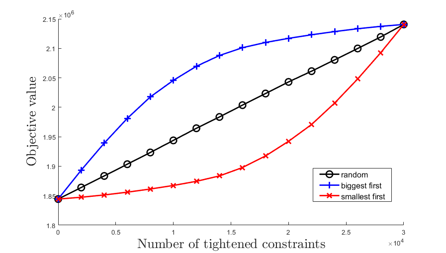
Figure 6: Separable-quadratic knapsack covering, $n=30,000$

LM1994 and SpeakmanYuLee suggested that for a pair of relaxations $P,Q\subset\mathbb{R}^{d}$, a good measure for evaluating $Q$ relative to $P$ might be $\sqrt[d]{\operatorname{vol}(Q)}-\sqrt[d]{\operatorname{vol}(P)}$ (in our present setting, we have $d=3$). We did experiments ranking by this, rather then the simpler $\operatorname{vol}(Q)-\operatorname{vol}(P)$, and we found no significant difference in our results. This can be explained by the fact that ranking by either of these choices is very similar for our test set. In Figure 7, we have a scatter plot of $\operatorname{vol}(Q)-\operatorname{vol}(P)$ vs. $\sqrt[d]{\operatorname{vol}(Q)}-\sqrt[d]{\operatorname{vol}(P)}$, across the $n=30,000$ choice of $u_{i}$ and $\ell_{i}$ from our experiment above. We can readily see that ranking by either of these choices is very similar.

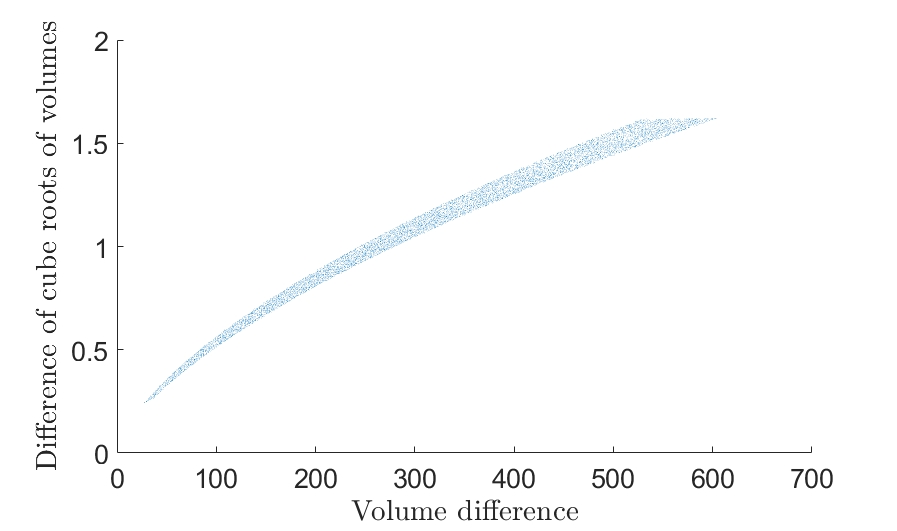
Figure 7: How to use volumes: Separable-quadratic knapsack covering, $n=30,000$

More precisely, the Kendall and Spearman rank correlation coefficients (“Kendall’s $\tau$” and “Spearman’s $\rho$”: non-parametric statistics used to measure ordinal association between two measured quantities) are 0.9647 and 0.9984, respectively. Notably the same numbers, measuring a relationship between either of our two quantities and the $u_{i}-\ell_{i}$ are all below 0.07, indicating that $u_{i}-\ell_{i}$ is not a good substitute for our measures based on volumes. Of course this is related to the fact that we (purposely) generated our data so that the $u_{i}-\ell_{i}$ has low variation.

5.2 Mean-variance optimization.

Next, we conducted a similar experiment on a richer model, though at a smaller scale. Our model is for a (Markowitz-style) mean-variance optimization problem (see gunlind1 and Frangioni2006 ). We have $n$ investment vehicles. The vector $\mathbf{a}$ contains the expected returns for the portfolio/holdings $\mathbf{x}$. The scalar $b$ is our requirement for the minimum expected return of our portfolio. Asset $i$ has a possible range $[\ell_{i},u_{i}]$, and we limit the number of assets that we hold to $\kappa$.

Variance is measured, as usual, via a quadratic which is commonly taken to have the form: $\mathbf{x}^{\prime}\left(\mathbf{Q}+\operatorname{Diag}(\mathbf{c})\right)\mathbf{x}$, where $\mathbf{Q}$ is positive definite and $\mathbf{c}$ is all positive (see gunlind1 and Frangioni2006 for details on why this form is used in the application). Taking the Cholesky factorization $\mathbf{Q}=\mathbf{M}\mathbf{M}^{\prime}$, we define $\mathbf{w}:=\mathbf{M}^{\prime}\mathbf{x}$, and introduce the scalar variable $v$. In this way, we arrive at the model:

$$\min\ v+\mathbf{c}^{\prime}\mathbf{y}$$

subject to:

$$\mathbf{a}^{\prime}\mathbf{x}\geq b~{};$$

$$\mathbf{e}^{\prime}\mathbf{z}\leq\kappa~{};$$

$$\mathbf{w}-\mathbf{M}^{\prime}\mathbf{x}=\mathbf{0}~{};$$

$$v\geq\|\mathbf{w}\|^{2}~{};$$

$$u_{i}z_{i}\geq x_{i}\geq\ell_{i}z_{i}~{},\qquad i=1,\ldots,n~{};$$

$$u_{i}^{2}z\geq y_{i}\geq x_{i}^{2}~{},\qquad i=1,\ldots,n~{};$$

$$1\geq z_{i}\geq 0,\qquad i=1,\ldots,n~{};$$

$$w_{i}\mbox{ unrestricted},\qquad i=1,\ldots,n~{}.$$

Note: The inequality $v\geq\|\mathbf{w}\|^{2}$ is correct; there is a typo in gunlind1 , where it is written as $v\geq\|\mathbf{w}\|$. The inequality $v\geq\|\mathbf{w}\|^{2}$, while not formulating a Lorentz (second-order) cone, may be re-formulated as an affine slice of a rotated Lorentz cone, or not, depending on the solver employed.

Most of our parameters are the same as for our first experiment. Here we took $n=1,500$ (these are harder models), and $\kappa:=\lfloor 0.8n\rfloor$. The remaining parameter is the lower-triangular matrix $M$, which we took to have independent entries distributed as $\mathcal{U}(0,0.0025)$.

Our results, summarized in Figure 8, follow the same general trend as Figure 6, again agreeing with the prediction of Corollary 6.

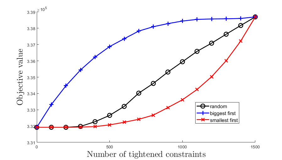
Figure 8: Mean-variance optimization: $n=1,500$

6 Concluding remarks

In general, we have presented three possibilities of relaxation:

• The weakest is the naïve relaxation, and it is the least computationally burdensome, amenable to general NLP solvers (like Ipopt or Knitro).

• Next tightest is the naïve relaxation applied to the tightened function $g$ (as defined in Lemma 6). This one, in the context of convex-optimization solvers, sometimes requires special handling for piecewise functions (see comments between Theorem 3.7 and Corollary 8).

• Finally, the tightest is the perspective relaxation, but this feature best lends itself to reliable solution using conic solvers (like Mosek and SDPT3), and only when the appropriate cone is supported by the solver. Presently, restriction to conic solvers limits the kinds of other functions that can be present in a model.

Furthermore, for power functions, we give a continuum of further possibilities, also best exploited using conic solvers.

As the solver landscape is rapidly changing, we do not have a uniform answer to the question of which model and solver to use. As we have demonstrated with our limited experiments, even for a fixed solver, our results can give some useful guidance in model choice. Going forward, we do hope and believe that our approach can be used by modelers and solver developers in their work.

References

- (1) Aktürk, M.S., Atamtürk, A., Gürel, S.: A strong conic quadratic reformulation for machine-job assignment with controllable processing times. Operations Research Letters 37(3), 187–191 (2009)
- (2) Basu, A., Conforti, M., Di Summa, M., Zambelli, G.: Optimal cutting planes from the group relaxations. Mathematics of Operations Research 44(4), 1208–1220 (2019)
- (3) Bertsekas, D.P.: Nonlinear programming, third edn. Athena Scientific Optimization and Computation Series. Athena Scientific, Belmont, MA (2016)
- (4) Chares, P.R.: Cones and interior-point algorithms for structured convex optimization involving powers and exponentials. Docteur en Sciences de l’Ingénieur, Université catholique de Louvain (2007)
- (5) Clark, P.L.: Honors Calculus (2014). math.uga.edu/~pete/2400full.pdf
- (6) Dey, S.S., Molinaro, M.: Theoretical challenges towards cutting-plane selection. Mathematical Programming 170(1), 237–266 (2018)
- (7) Frangioni, A., Gentile, C.: Perspective cuts for a class of convex 0–1 mixed integer programs. Mathematical Programming 106(2), 225–236 (2006)
- (8) Grant, M., Boyd, S.: CVX: Matlab software for disciplined convex programming, version 2.1, build 1123. http://cvxr.com/cvx (2017)
- (9) Günlük, O., Linderoth, J.: Perspective reformulations of mixed integer nonlinear programs with indicator variables. Mathematical Programming, Series B 124, 183––205 (2010)
- (10) Hiriart-Urruty, J.B., Lemaréchal, C.: Convex analysis and minimization algorithms. I: Fundamentals, Grundlehren der Mathematischen Wissenschaften, vol. 305. Springer-Verlag, Berlin (1993)
- (11) Ko, C.W., Lee, J., Steingrímsson, E.: The volume of relaxed Boolean-quadric and cut polytopes. Discrete Mathematics 163(1-3), 293–298 (1997)
- (12) Lee, J.: Mixed integer nonlinear programming: Some modeling and solution issues. IBM Journal of Research and Development 51(3/4), 489–497 (2007)
- (13) Lee, J., Morris Jr., W.D.: Geometric comparison of combinatorial polytopes. Discrete Applied Mathematics 55(2), 163–182 (1994)
- (14) Lee, J., Skipper, D.: Virtuous smoothing for global optimization. Journal of Global Optimization 69(3), 677–697 (2017)
- (15) Lee, J., Skipper, D.: Volume computation for sparse boolean quadric relaxations. To appear in: Discrete Applied Mathematics (2017). Doi:10.1016/j.dam.2018.10.038
- (16) MOSEK ApS: MOSEK Modeling Cookbook, Release 3.1 (2019). https://docs.mosek.com/MOSEKModelingCookbook-letter.pdf
- (17) Speakman, E., Averkov, G.: Computing the volume of the convex hull of the graph of a trilinear monomial using mixed volumes. Discrete Applied Mathematics (2019). To appear
- (18) Speakman, E., Lee, J.: Quantifying double McCormick. Mathematics of Operations Research 42(4), 1230–1253 (2017)
- (19) Speakman, E., Lee, J.: On branching-point selection for trilinear monomials in spatial branch-and-bound: the hull relaxation. Journal of Global Optimization 72(2), 129–153 (2018)
- (20) Speakman, E., Yu, H., Lee, J.: Experimental validation of volume-based comparison for double-McCormick relaxations. In: D. Salvagnin, M. Lombardi (eds.) CPAIOR 2017, pp. 229–243. Springer (2017)
- (21) Speakman, E.E.: Volumetric guidance for handling triple products in spatial branch-and-bound. Ph.D., University of Michigan (2017)
- (22) Steingrímsson, E.: A decomposition of -weak vertex-packing polytopes. Discrete & Computational Geometry. 12(4), 465–479 (1994)
- (23) Toh, K.C., Todd, M.J., Tütüncü, R.H.: SDPT3 - a MATLAB software package for semidefinite programming. Optimization Methods and Software 11, 545–581 (1998)
- (24) Xu, L., Lee, J., Skipper, D.: More virtuous smoothing. SIAM Journal on Optimization 29(2), 1240–1259 (2019)