Frequency Fitness Assignment: Making Optimization Algorithms Invariant under Bijective Transformations of the Objective Function Value

Abstract

Under Frequency Fitness Assignment (FFA), the fitness corresponding to an objective value is its encounter frequency in fitness assignment steps and is subject to minimization. FFA renders optimization processes invariant under bijective transformations of the objective function value. On TwoMax, Jump, and Trap functions of dimension s, the classical (1+1)-EA with standard mutation at rate 1/s can have expected runtimes exponential in s. In our experiments, a (1+1)-FEA, the same algorithm but using FFA, exhibits mean runtimes that seem to scale as s² ln s. Since Jump and Trap are bijective transformations of OneMax, it behaves identical on all three. On OneMax, LeadingOnes, and Plateau problems, it seems to be slower than the (1+1)-EA by a factor linear in s. The (1+1)-FEA performs much better than the (1+1)-EA on W-Model and MaxSat instances. We further verify the bijection invariance by applying the Md5 checksum computation as transformation to some of the above problems and yield the same behaviors. Finally, we show that FFA can improve the performance of a memetic algorithm for job shop scheduling.

I Introduction

Fitness assignment is a component of many Evolutionary Algorithms (EAs). It transforms the features of candidate solutions, such as their objective value(s), to scalar values which are then the basis for selection. Frequency Fitness Assignment (FFA) [1, 2] was developed to enable algorithms to escape from local optima. In FFA, the fitness corresponding to an objective value is its encounter frequency so far in fitness assignment steps and is subject to minimization. As we discuss in detail in Section II, FFA turns a static optimization problem into a dynamic one where objective values that are often encountered will receive worse and worse fitness.

In this article, we uncover a so-far unexplored property of FFA: It is invariant under any bijective transformation of the objective function values. This is the strongest invariance known to us and encompasses all order-preserving mappings. Other examples for bijective transformations include the negation, permutation, or even encryption of the objective values. According to [3], invariance extends performance observed on a single function to an entire associated invariance class, that is, it generalizes from a single problem to a class of problems. Thus it hopefully provides better robustness w.r.t. changes in the presentation of a problem. FFA generalizes the performance of an algorithm on OneMax to all problems which are bijections thereof, including Jump and Trap.

While invariances are generally beneficial for optimization algorithms [4, 5], such strong invariance comes at a cost: The idea that solutions of better objective values should be preferred to those with worse ones can no longer be applied, since many bijections are not order-preserving. FFA only considers whether objective values are equal or not. One would expect that this should lead to a loss of performance. We find that the opposite is the case on several benchmarks evaluated in our study. On those where FFA increases the number of function evaluations (FEs) to find the optimum, i.e., the runtime, it seems to do so only linearly with the number of different objective values or the problem dimension $s$, as both cases are indistinguishable in the investigated problems.

We plug FFA into the most basic EA [6], the (1+1)-EA with standard mutation at rate $1/s$, and obtain the (1+1)-FEA. We investigate its performance on several well-known problems, namely the OneMax, LeadingOnes, TwoMax, Jump, Trap, and Plateau functions, the W-Model, and MaxSat, all defined over bit strings of length $s$. We find that the resulting (1+1)-FEA is slower on OneMax, LeadingOnes, and on the Plateau functions, while it very significantly reduces the runtime needed to solve the other problems. Most notably, in our experiments, it has runtime requirements in the scale of $s^{2}\ln{s}$ on the TwoMax, Trap and Jump problems, for which the expected runtime needed by the (1+1)-EA to find the global optimum is in ${\mathbf{\Omega}}\!\left(s^{s}\right)$, ${\mathbf{\Theta}}\!\left(s^{s}\right)$, and ${\mathbf{\Theta}}\!\left(s^{w}+s\ln{s}\right)$ (for jump width $w$) FEs, respectively. We confirm the invariance under bijections of the objective value by solving several benchmark problems with the (1+1)-FEA by optimizing the Md5 checksums, i.e., cryptographic hashes, of their objective values and observing no change in algorithm behavior. We also explore plugging FFA into a well-performing algorithm for a job shop scheduling problem, where it can improve the result quality under budget constraints.

In Section II, we discuss the invariance property of FFA and how FFA can be plugged into the (1+1)-EA. Related works are discussed in Section III. Our comprehensive experimental study is given in Section IV. We conclude our article and give pointers to future work in Section V.

II Frequency Fitness Assignment

This study investigates the impact of FFA when plugged into the maybe most basic EA, the (1+1)-EA. The (1+1)-EA starts with a random bit string $x_{c}$ of length $s$. Until the termination criterion is met, in each step, it applies the standard mutation operator, where each of the $s$ bits of $x_{c}$ is flipped independently with probability $1/s$ and the result is a new string $x_{n}$. If $x_{n}$ is at least as good as $x_{c}$, it replaces $x_{c}$. The expected runtime of the (1+1)-EA for an arbitrary objective function is at most $s^{s}$ [7]. Some of the benchmark problems we investigate invoke this boundary.

We apply a slight modification of the (1+1)-EA, called the $\mbox{(1+1)-\mbox{{EA}}}_{>0}$ [8]: The standard mutation in each iteration is repeated until at least one bit is flipped [9]. No FE is wasted by evaluating a candidate solution identical to the current one. The probability of this in the (1+1)-EA is $\left(1-s^{-1}\right)^{s}$, which approaches $1/e\approx 0.368$ for $s\rightarrow\infty$. This small change thus saves more than one third of the FEs while not changing any other characteristic of the algorithm [8, 10]. In the following text, expected runtimes for the (1+1)-EA will therefore be corrected by factor $1\!-\!\left(1\!-\!s^{-1}\right)^{s}$ to hold for the $\mbox{(1+1)-\mbox{{EA}}}_{>0}$ where necessary.

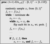
(a) $\mbox{(1+1)-\mbox{{EA}}}_{>0}$

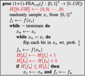
(b) $\mbox{(1+1)-\mbox{{FEA}}}_{>0}$

Figure 1: The simplified pseudo codes of the $\mbox{(1+1)-\mbox{{EA}}}_{>0}$ and the $\mbox{(1+1)-\mbox{{FEA}}}_{>0}$, which applies FFA, for minimization problems. Differences are marked in red. Note: In an actual implementation, the algorithms would remember and return the candidate solution with the best encountered objective value $f_{\textnormal{B}}$ (not fitness).

In Figure 1, we put the pseudo code of the $\mbox{(1+1)-\mbox{{EA}}}_{>0}$ next to a simplified version of the $\mbox{(1+1)-\mbox{{FEA}}}_{>0}$. We assume that

1. the objective function $f$ is subject to minimization, that

2. its upper bound $U\!B$ is known, that

3. all objective values are integers greater or equal to 0, and that

4. the solution space is $\mbox{$\{0,1\}$}^{s}$, the bit strings of length $s$.

This can be established for many well-known benchmark problems on which the (1+1)-EA is usually investigated, as well as for many practical optimization problems like MaxSat.

Under these assumptions, only minimal changes to the $\mbox{(1+1)-\mbox{{EA}}}_{>0}$ are necessary to introduce FFA: An array $H$ of integers of length $\mbox{$U\!B$}+1$ is used to hold the frequency of each objective value in $[0..\mbox{$U\!B$}]$. Before selecting one of the two candidate solutions with objective values $f_{c}$ and $f_{n}$, the frequencies $H\!\left[\mbox{$f_{c}$}\right]$ and $H\!\left[\mbox{$f_{n}$}\right]$ of these objective values are increased. The results of these increments are compared. Note: Both frequencies are increased, because if $H\!\left[\mbox{$f_{c}$}\right]$ was not incremented, solutions with unique objective values could become traps for the optimization process.

In order to conduct an efficient search under FFA, the set ${\mathbb{Y}}$ of possible objective values for the problem to be solved should not be too big. FFA must maintain a frequency table $H$, which has the same size as $\mathbb{Y}$. Also, FFA attempts to distribute the search effort evenly over all objective values. In the extreme case where each distinct solution has a different objective value, FFA almost degenerates the search to a random walk.

Most often, the (1+1)-EA is analyzed as maximization algorithm. Since the (1+1)-FEA minimizes the objective value frequencies, we also present the (1+1)-EA for minimization and define the benchmark problems in Section IV accordingly.

The (1+1)-FEA implementation given in Figure 1b can easily be extended towards a ($\mu$+$\lambda$)-EA. It can also be modified to handle problems with unknown upper and lower bounds of the objective function (or objective functions that return real numbers but can still be discretized) by implementing $H$ as hash table [11] (see Section IV-G). FFA can be introduced into arbitrary metaheuristics.

Theorem 1

The sequence of candidate solutions $x\in\mathbb{X}$ generated by an optimization process applying FFA is invariant under any bijection $g:\mathbb{Y}\rightarrow\mathbb{Z}$ of the objective function $f:\mathbb{X}\rightarrow\mathbb{Y}$, where $\mathbb{X}$ is the solution space, $\mathbb{Y}$ is a finite subset of $\mathbb{R}$, and $\mathbb{Z}$ is a set of the same size.

Proof:

The bijection $g$ maps each value from $\mathbb{Y}$ to one value in $\mathbb{Z}$ and vice versa. Therefore, if two objective values identify the same (or a different) entry in $H$, so will their bijective transformations. Under FFA, only the entries in $H$ are modified and compared to make selection decisions.∎

We can also prove this inductively: Assume that two runs of the $\mbox{(1+1)-\mbox{{FEA}}}_{>0}$ which minimize $f$ and $g\circ f$, respectively, are identical until iteration $t$: They have the same random seed, same $x_{c}$, and $\mbox{$H\!\left[y\right]$}=\mbox{$H^{\prime}\!\left[g(y)\right]$}\forall y\in\mathbb{Y}$ holds for their respective FFA tables. Both will sample the same next point $x_{n}$. $\mbox{$H\!\left[\mbox{$f\!\left(\mbox{$x_{c}$}\right)$}\right]$}=\mbox{$H^{\prime}\!\left[g(\mbox{$f\!\left(\mbox{$x_{c}$}\right)$})\right]$}$ and $\mbox{$H\!\left[\mbox{$f\!\left(\mbox{$x_{n}$}\right)$}\right]$}=\mbox{$H^{\prime}\!\left[g(\mbox{$f\!\left(\mbox{$x_{n}$}\right)$})\right]$}$ will still hold after incrementing the entries. Hence, both will make the same decision regarding the update of $x_{c}$ and begin iteration $t+1$ in the same state. In Sections IV-D, IV-E, and IV-G, we provide experimental evidence that this invariance indeed holds.

III Related Work

FFA was designed as an approach to prevent the premature convergence to a local optimum. In the context of EAs, it is therefore related to fitness sharing, niching, and clearing [12, 13]. Several such diversity-preserving mechanisms have been plugged into a ($\mu$+1)-EA and studied theoretically in [14] on TwoMax, where the original algorithm requires ${\mathbf{O}}\!\left(s^{s}\right)$ FEs to find the optimum. It is found that avoiding fitness or genotype duplicates does not help, whereas with deterministic crowding and sufficiently large $\mu$, the problem can be solved efficiently with high probability. With fitness sharing and $\mbox{$\mu$}\geq 2$, the ($\mu$+1)-EA can solve TwoMax in ${\mathbf{O}}\!\left(\mbox{$\mu$}s\log{s}\right)$. Different from the above methods, which only consider the current population, FFA tries to guide the search away from objective values that have been encountered often during the whole course of the optimization process. In Section IV-C, we will show that FFA can help solving TwoMax efficiently already at $\mbox{$\mu$}=1$.

Another related idea is Tabu Search (TS) [15], which improves local search by declaring solutions (or solution traits) which have already been visited as tabu, preventing them from being sampled again. Like FFA, it utilizes the search history, but usually in form of a list of tabu solutions or solution traits. Different from FFA, the TS relies on the order of objective values when deciding which solutions to accept.

The Fitness Uniform Selection Scheme (FUSS) [16] selects solutions in such a way that their corresponding objective values are approximately uniformly distributed within the range of the minimum and maximum objective value in the population. The Fitness Uniform Deletion Scheme (FUDS) [17] works similarly, but instead of selecting individuals, it deletes them when slots in the population are required to integrate the offspring. Both methods need populations, only consider the individuals in the current population, and are only invariant under translation and scaling of the objective function.

The ageing operator in Artificial Immune Systems (AIS) deletes individuals either after they have survived a certain number of iterations, with a certain probability, or both [18, 19, 20]. Ageing has also been applied in EAs [21]. Like FFA, ageing makes solutions less attractive if they remain in the population for a long time. Different from FFA, the information about these solutions disappears from the optimization process once they “die.”

Methods which try to balance between solution quality and population diversity are today grouped under the term Quality-Diversity (QD) algorithms [22, 23, 24].

Novelty Search (NS) [25] is a QD algorithm. Instead of an objective function $f$, NS uses a (dynamic) novelty metric $\rho$. This metric is computed, e.g., as mean behavior difference to the $k$ nearest neighbors in an archive of past solutions. FFA works on the original objective function and just transforms it to a dynamic fitness measure. It does not require an archive of solutions but uses a table $H$ counting the frequency of the objective values.

While NS was aimed to abandon the objective function $f$, using it as behavior definition was also tested [25]. Then, $\rho$ is the mean distance to $k$ neighbors (or all solutions ever found) in the objective space. Unlike FFA, this uses the assumption that differences between objective values are useful or correlate with diversity. Novelty Search with Local Competition (NSLC) [26] combines the search for finding diverse solutions with a local competition objective rewarding solutions which can outperform those most similar to them.

The MAP-Elites algorithm [27] combines a performance objective $f$ and a user-defined space of features that describe candidate solutions, which is not required by FFA. MAP-Elites searches for highest-performing solution in each cell of the discretized feature space.

Surprise Search (SS) [28] uses the concept of surprise as an alternative to novelty. A solution is scored by the difference of its observed behavior from the expected behavior. A history of discovered solution behaviors is maintained and used to predict the behavior of the new solutions. SS has also been combined with NSLC in a multi-objective fashion [22].

All of the above algorithms are conceptually different from FFA. They either are complete optimization methods (NS, QD, TS) or modules for EAs (FUSS/FUDS), while FFA can be plugged into many different optimization algorithms. Unlike FFA, none of the above methods exhibits an invariance under bijective transformations of the metrics they try to optimize.

From the perspective of invariances, FFA is related to Information-Geometric Optimization (IGO) [3]. IGO also replaces the objective function $f$ with an adaptive transformation of it. This transformation indicates how good or bad an objective value is relative to other observed objective values, i.e., is different from our method which simply compares encounter frequencies. IGO is invariant under all strictly increasing transformations of $f$, whereas FFA creates invariance under all bijective transformations. IGO is a complete family of optimization methods which can also exhibit invariance under several transformations of the search space. Since FFA only works on $f$, it cannot provide such invariances. IGO can optimize continuous objective functions, which is not possible with FFA.

IV Experiments

We now apply the $\mbox{(1+1)-\mbox{{EA}}}_{>0}$ and the $\mbox{(1+1)-\mbox{{FEA}}}_{>0}$ to minimization versions of different classical optimization problems. We initialize the $\mbox{(1+1)-\mbox{{EA}}}_{>0}$ and the $\mbox{(1+1)-\mbox{{FEA}}}_{>0}$ with the same random seeds for each run, i.e., we always have pairs of runs starting at the same random initial solution and sampling the same first offspring solutions for both algorithms.

The runs are terminated when they discover the optimum. In some experiments, we additionally limit the computational budget to $10^{10}=10^{\prime}000^{\prime}000^{\prime}000$ FEs. This should be enough to converge on problems that the algorithms can solve well, as can be seen in Section IV-B. Leading to several hours to more than a day for a single run on the corresponding problems, this was also the maximum budget we could feasibly allow.

Whenever all runs on an instance succeed to find the optimum, we can compare the mean runtime ‘$\textnormal{mean}(\mbox{{RT}})$’ they need to do so in terms of the consumed FEs (often called the first hitting time). When some runs fail in the budget-limited settings, we follow the approach from [29] and use the empirically estimated expected runtime (ERT) instead. The ERT for a problem instance is estimated as the ratio of the sum of all FEs that all the runs consumed until they either have discovered a global optimum or exhausted their budget, divided by the number of runs that discovered a global optimum [29]. The ERT is the mean expected runtime under the assumption of independent restarts after failed runs, which then may either succeed (consuming the mean runtime of the successful runs) or fail again (with the observed failure probability, after consuming ${10}^{10}$ FEs).

In order to guarantee the reproducibility of our work, we provide the complete data used in this paper, including the result log files, the scripts used to generate all the figures and tables, as well as the source code of all algorithms and all benchmark problems in [30].

IV-A OneMax Problems

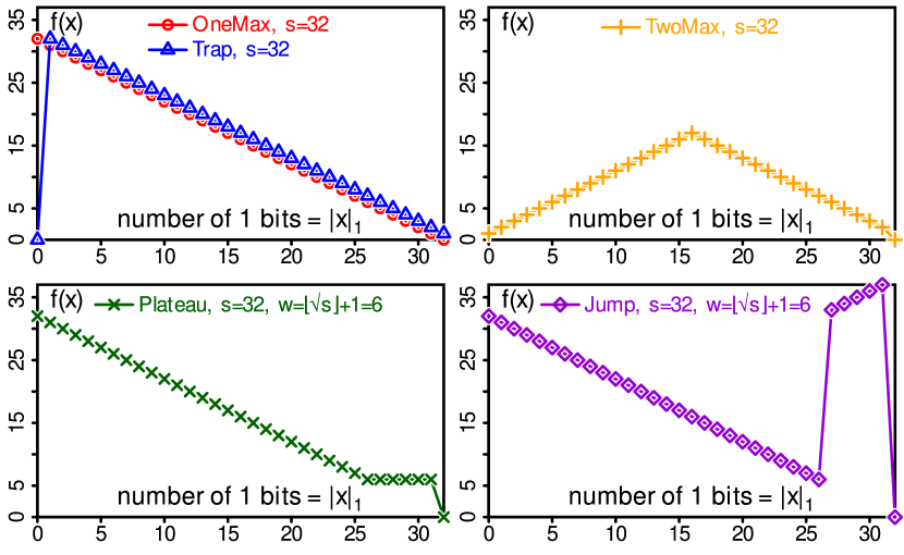
Figure 2: Illustrations of the OneMax, TwoMax, Trap, Jump, and Plateau problems for $s=32$ and $\mbox{$w$}=6$.

OneMax [9] is a unimodal optimization problem where the goal is to discover a bit string of all ones. Its minimization version of dimension $s$ is defined below and illustrated in Figure 2:

$$\mbox{OneMax}(x)=s-\mbox{$\left|x\right|_{1}$}\textnormal{~{}where~{}}\mbox{$\left|x\right|_{1}$}=\sum_{i=1}^{s}\mbox{$x\!\left[i\right]$}$$ (1)

It has a black-box complexity of ${\mathbf{\Omega}}\!\left(s/\ln{s}\right)$ [31, 32]. Here, an (1+1)-EA has an expected runtime of ${\mathbf{\Theta}}\!\left(s\ln{s}\right)$ FEs [9]. A very exact formula [33] with our correction factor for the $\mbox{(1+1)-\mbox{{EA}}}_{>0}$ is given in Equation (2), where $C_{1}\approx 1.89254$ and $C_{2}\approx 0.59789875$.

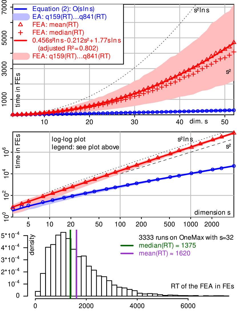
Figure 3: The runtime measured for the $\mbox{(1+1)-\mbox{{EA}}}_{>0}$ and $\mbox{(1+1)-\mbox{{FEA}}}_{>0}$ on selected instances of the OneMax problem.

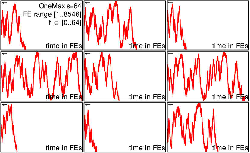
Figure 4: 9 typical runs of $\mbox{(1+1)-\mbox{{FEA}}}_{>0}$ on OneMax ($s=64$)

We conduct 3333 runs with both the $\mbox{(1+1)-\mbox{{EA}}}_{>0}$ and $\mbox{(1+1)-\mbox{{FEA}}}_{>0}$ on this problem for each $s\in[3..333]$ and 71 runs for 26 selected larger values of $s$ up to 4096, all without budget constraint. In Figure 3, we illustrate the mean runtime to solve the instances with the range of the 15.9% to the 84.1% quantiles in the background. In the top-most sub-figure, we illustrate all results for $s\in[3..52]$. The middle figure is a log-log plot based on the complete data, but with marks only placed at $s\in\{2^{i},round(2^{i}/3)\}$ to not clutter the plot. In both diagrams, we illustrate the results of Equation (2) without the ${\mathbf{O}}\!\left((\ln{s})/s\right)$ term. They exactly match the results of the $\mbox{(1+1)-\mbox{{EA}}}_{>0}$.

The mean runtime of the $\mbox{(1+1)-\mbox{{FEA}}}_{>0}$ seems to be in the scale of $s^{2}\ln{s}$ for the investigated range of $s$. The illustrated model was obtained using linear regression on the complete set of 1’105’069 runs with the inverse variances of the measured runtimes per distinct $s$ value used as weights. All regression models in the rest of this article are obtained in the same way. The curve of the model visually fits to the mean runtimes and the adjusted $R^{2}$ value of $0.8$ indicates that it can explain most of the variance in the data.

The observed distribution of the runtime is skewed and the median is lower than the mean on all dimensions. This is illustrated exemplarily in the histogram for dimension $s=32$ in the lower part of Figure 3. Its shape resembles a log-normal distribution or a sum of parameterized geometric distributions [34]. For $s\leq 8$, the histograms look like exponential distributions, caused by the high chance of randomly guessing the optimum.

Figure 4 illustrates nine typical runs of the $\mbox{(1+1)-\mbox{{FEA}}}_{>0}$ on the OneMax problem with $s=64$. Initially, some of the runs progress towards better solutions, others to worse. They change the search direction from time to time. This oscillation is repeated until the global optimum is discovered.

IV-B LeadingOnes Problems

The LeadingOnes problem [4, 35] maximizes the length of a leading sequence containing only 1 bits. Its minimization version of dimension $s$ is defined as follows:

$$\mbox{LeadingOnes}(x)=s-\sum_{i=1}^{s}\prod_{j=1}^{i}\mbox{$x\!\left[j\right]$}$$ (3)

The problem exhibits epistasis, as the bit at index 2 can only contribute to the objective value if the bit at index 1 has value 1. The black-box complexity of LeadingOnes is ${\mathbf{\Theta}}\!\left(s\ln{\ln{s}}\right)$ [36]. The (1+1)-EA has a quadratic expected runtime on LeadingOnes [7]. The exact formula [37, 38] is presented with our correction factor in Equation (4):

$${\color[rgb]{.5,0,.5}\left[\mbox{{\color[rgb]{.5,0,.5}$1\!-\!\left(1\!-\!s^{-1}\right)^{s}$}}\right]}\left[0.5s^{2}\left(\left(1-1/s\right)^{1-s}-1+1/s\right)\right]$$ (4)

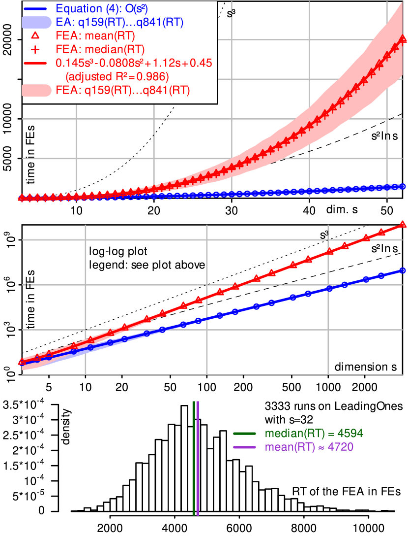
Figure 5: The runtime measured for the $\mbox{(1+1)-\mbox{{EA}}}_{>0}$ and $\mbox{(1+1)-\mbox{{FEA}}}_{>0}$ on the LeadingOnes problem.

Figure 5 has the same structure as Figure 3 and is based on an experiment with the same parameters, only using the LeadingOnes instead of the OneMax problem. The $\mbox{(1+1)-\mbox{{EA}}}_{>0}$ behaves as predicted in Equation (4).

The runtime of the $\mbox{(1+1)-\mbox{{FEA}}}_{>0}$ fits to the illustrated regression model for the investigated range of $s$ and can explain almost all of the variance of the data. Due to the approximately cubic runtime, the mean time to solve LeadingOnes at $s=4096$ is $9.9\!\cdot\!10^{9}$ FEs. The histogram of the observed runtimes for dimension $s=32$ in the lower part of Figure 5 is slightly skewed.

IV-C TwoMax Problems

The minimization version of the TwoMax [39, 40] problem of dimension $s$ can be defined as follows:

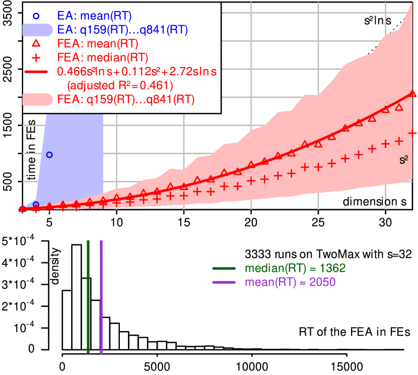
Figure 6: The runtime measured for the $\mbox{(1+1)-\mbox{{EA}}}_{>0}$ and $\mbox{(1+1)-\mbox{{FEA}}}_{>0}$ on the TwoMax problem.

The TwoMax problem introduces deceptiveness in the objective function by having a local and a global optimum. Since their basins of attraction have the same size, a (1+1)-EA can solve the problem in ${\mathbf{\Theta}}\!\left(s\ln{s}\right)$ steps with probability 0.5 while otherwise needing exponential runtime. The resulting overall expected runtime is in ${\mathbf{\Omega}}\!\left(s^{s}\right)$ [14, 39].

On each instance of TwoMax with $s\in[3..32]$, we conduct 71 runs with $\mbox{(1+1)-\mbox{{EA}}}_{>0}$ and 3333 with $\mbox{(1+1)-\mbox{{FEA}}}_{>0}$. For all experiments from here on except in Section IV-J, we use a budget of ${10}^{10}$ FEs. The $\mbox{(1+1)-\mbox{{EA}}}_{>0}$ succeeds in solving the problem only in about half of the runs for $s>10$ within the budget, which was the reason for the 71-run limit. We illustrate its performance in Figure 6 only for dimensions $s<10$ where it always succeeded.

All runs of $\mbox{(1+1)-\mbox{{FEA}}}_{>0}$ solved their corresponding instances. The algorithm exhibits a mean runtime fitting to a model of scale $s^{2}\ln{s}$ for $s\in[3..32]$, which is a big improvement in comparison to the exponential time needed by the (1+1)-EA. The lower adjusted $R^{2}$ and less smooth increase of the runtime with $s$ result from the slightly different shapes of the TwoMax problem for odd and even values of $s$. The median runtime is again smaller than the mean. The histogram of the observed runtimes for $s=32$ in the lower part of Figure 6 again exhibits the familiar skew.

These results are interesting, since avoiding fitness duplicates in a ($\mu$+1)-EA does not help to solve the problem efficiently [14]. FFA thus does more than this even at $\mbox{$\mu$}=1$.

IV-D Jump Problems

The Jump functions as defined in [7, 39] introduce a deceptive region of width $w$ with very bad objective values right before the global optimum. The minimization version of the Jump function of dimension $s$ and jump width $w$ is defined as follows:

$$\mbox{Jump}(x)=\left\{\!\!\!\begin{array}[]{l@{~}l}s-\mbox{$\left|x\right|_{1}$}\hfil~{}&\textnormal{if }\left(\mbox{$\left|x\right|_{1}$}=s\right)\lor\left(\mbox{$\left|x\right|_{1}$}\leq s-\mbox{$w$}\right)\\ \mbox{$w$}+\mbox{$\left|x\right|_{1}$}\hfil~{}&\textnormal{otherwise}\end{array}\right.$$ (6)

The expected runtime of the (1+1)-EA on such problems is in ${\mathbf{\Theta}}\!\left(s^{w}+s\ln{s}\right)$ [7]. The Jump problem is a bijective transformation of the OneMax problem. The $\mbox{(1+1)-\mbox{{FEA}}}_{>0}$ will exhibit the same behavior and runtime requirement on any jump problem instance as on a OneMax instance of the same dimension $s$, regardless of the jump width $w$.

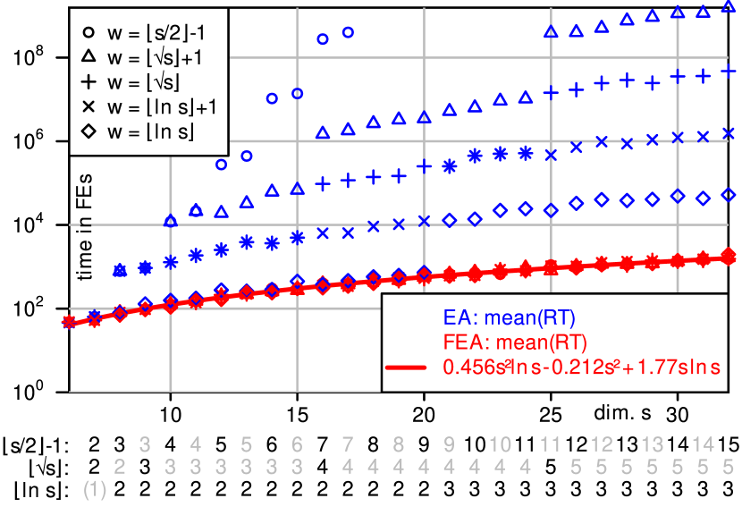
Figure 7: The runtime measured for the $\mbox{(1+1)-\mbox{{EA}}}_{>0}$ and $\mbox{(1+1)-\mbox{{FEA}}}_{>0}$ on Jump problems with dimension $s$ and jump width $\mbox{$w$}>1$.

We conduct experiments with five different jump widths $w$, namely $\left\lfloor\ln{s}\right\rfloor$, $\left\lfloor\ln{s}\right\rfloor+1$, $\left\lfloor\sqrt{s}\right\rfloor$, $\left\lfloor\sqrt{s}\right\rfloor+1$, and $\left\lfloor 0.5s\right\rfloor-1$. We illustrate the results in Figure 7 only for those setups where a success rate of 100% within the $10^{10}$ FEs were achieved in 71 runs. $\mbox{(1+1)-\mbox{{FEA}}}_{>0}$ finds the optimum in all runs and all the observed mean runtimes fall on the function fitted to the results on OneMax (see Figure 3), confirming that the two problems are indeed identical from the perspective of an algorithm using FFA. As expected, the runtime of the $\mbox{(1+1)-\mbox{{EA}}}_{>0}$ steeply increases with the jump width $w$ and it is outperformed by the $\mbox{(1+1)-\mbox{{FEA}}}_{>0}$.

Depending on its configuration, the AIS Opt-IA [18] needs runtimes of at least ${\mathbf{O}}\!\left(s^{2}\ln{s}\right)$ and ${\mathbf{O}}\!\left(s^{3}\right)$ FEs on OneMax and LeadingOnes, respectively. It seems that our (1+1)-FEA has similar requirements, i.e., compared to the (1+1)-EA with standard bit mutation, a linear slowdown is incurred on these problems. However, on the Jump problems, Opt-IA needs, again depending on its configuration, at least ${\mathbf{O}}\!\left(\frac{s^{w+1}\cdot e^{w}}{w^{w}}\right)$ FEs. The (1+1) Fast-IA [19], which is at least as fast as the (1+1)-EA on OneMax and LeadingOnes, needs exponential expected runtime for sufficiently large $w$. The Fast EA [42] using a heavy-tailed mutation rate, too, needs exponential runtime to solve Jump. The asymptotic performance of the cGA on Jump is not worse than on OneMax for logarithmic jump widths $w$ [43], but it still needs exponential time for larger $w$ [44]. (1+1)-FEA, however, performs on Jump exactly as on OneMax, regardless of $w$.

IV-E Trap Function

The Trap function [45, 7] is very similar to the OneMax problem, except that it replaces the worst possible solution there with the global optimum. Following a path of improving objective values will always lead the optimization algorithm away from the global optimum. The (1+1)-EA here has an expected runtime of ${\mathbf{\Theta}}\!\left(s^{s}\right)$ [7]. The minimization version of the Trap function can be specified as follows:

$$\mbox{Trap}(x)=\left\{\!\!\!\begin{array}[]{l@{~}l}0\hfil~{}&\textnormal{if~{}}\mbox{$\left|x\right|_{1}$}=0\\ s-\mbox{$\left|x\right|_{1}$}+1\hfil~{}&\textnormal{otherwise}\end{array}\right.$$ (7)

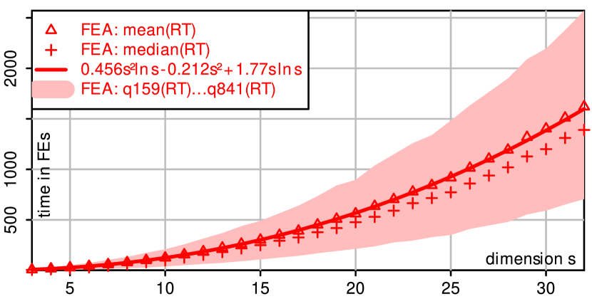
Figure 8: The runtime measured for the $\mbox{(1+1)-\mbox{{FEA}}}_{>0}$ on the Trap problem.

The Trap function is another bijective transformation of the OneMax problem. When we plot the results from 3333 runs of the $\mbox{(1+1)-\mbox{{FEA}}}_{>0}$ on the Trap function in Figure 8, we find that the results are almost exactly identical to those obtained on OneMax and illustrated in Figure 3. The function fitted to the mean runtime on OneMax, again plotted in Figure 8, passes through the points measured on the Trap function.

IV-F Plateau Problems

The minimization version of the Plateau [46] function of dimension $s$ with plateau width $w$ is defined as follows:

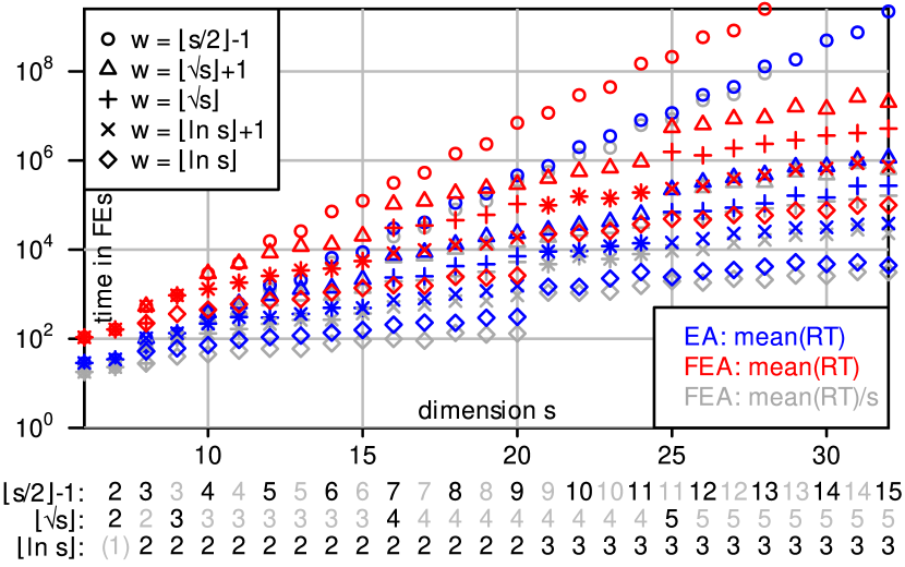
Figure 9: The runtime measured for the $\mbox{(1+1)-\mbox{{EA}}}_{>0}$ and $\mbox{(1+1)-\mbox{{FEA}}}_{>0}$ on Plateau problems with dimension $s$ and plateau width $\mbox{$w$}>1$.

The expected runtime of the (1+1)-EA on such a problem is in ${\mathbf{\Theta}}\!\left(s^{w}\right)$ [46]. The Plateau problems are no bijective transformation of OneMax. Instead, they reduce the number of possible objective values ($|\mathbb{Z}|<|\mathbb{Y}|$). We can expect that the fitness of the solutions on the plateau will get worse quickly under FFA. We conduct the same experiment as for the Jump function with the Plateau function and plot the results in the same manner in Figure 9. This time, the $\mbox{(1+1)-\mbox{{FEA}}}_{>0}$ performs worse than the (1+1)-EA. Interestingly, if we divide the observed mean runtimes of $\mbox{(1+1)-\mbox{{FEA}}}_{>0}$ by the problem dimension $s$, we approximately obtain those observed with $\mbox{(1+1)-\mbox{{EA}}}_{>0}$ (see the gray marks in Figure 9). This might be a coincidence and more research is necessary.

IV-G Bijection Invariance: Md5 Checksum of Objective Values

We now repeat our experiments with the $\mbox{(1+1)-\mbox{{FEA}}}_{>0}$ on the OneMax, TwoMax, LeadingOnes, and Trap problems with $s\in[3..32]$, but use a transformation of the objective functions: Instead of working on the objective values directly, we optimize their Md5 checksums. We therefore implement $H$ as a hash table where their encounter frequencies are stored. The Md5 checksum is a 128 bit message digest published in [47], where it is conjectured that it is computationally infeasible to produce two messages having the same message digest. Although Md5 checksums are not an encryption method, they do allow us to further test the invariance under such “extreme” transformations and the idea of implementing $H$ as hash table without further assumptions.

We use the same random seeds as in the original runs working on the objective values. We find that all 3333 runs on all the instances have the same (FE, objective value)-traces as their counterparts, which also follows from Theorem 1. Illustrating these results here has no merit, as the figures would be identical to those already shown. We include the full log files as well as the algorithm implementation in our dataset [30].

IV-H W-Model Instances

The W-Model [48, 49, 50] is a benchmark problem which exhibits different difficult fitness landscape features in a tunable fashion. These include the base size (via parameter $n$), neutrality (via parameter $m$), epistasis (via parameter $\nu$), and ruggedness (via parameter $\gamma$), from which instances of dimension $s=mn$ result. The W-Model base problem is equivalent to OneMax but searches for a string of alternating 0 and 1 bits. Different transformations are applied to it. While the ruggedness transformation is a bijective transformation of objective function, the mappings introducing neutrality and epistasis transform the search space itself. 19 diverse W-Model instances have been selected in [51] based on a large-scale experiment. No theoretical bounds for the runtimes on these instances are known, but they exhibit different degrees of empirical hardness for different algorithms.

TABLE I: The ERT and fraction fs of the 71 $\mbox{(1+1)-\mbox{{EA}}}_{>0}$ runs discovering the optimum on the 19 W-Model problem instances selected in [51]. As all runs of $\mbox{(1+1)-\mbox{{FEA}}}_{>0}$ reached the optimum, we present its mean and median runtime.

0pt W-Model Instance $\mbox{(1+1)-\mbox{{EA}}}_{>0}$ $\mbox{(1+1)-\mbox{{FEA}}}_{>0}$ id $n$ $m$ $\nu$ $\gamma$ fs ERT $\textnormal{mean}(\mbox{{RT}})$ $\textnormal{med}(\mbox{{RT}})$ 1 10 2 6 10 1 5’928 1’090 734 2 10 2 6 18 1 6’605 904 815 3 16 1 5 72 1 9’400 3’646 3’191 4 16 3 9 72 1 864’850 5’856 5’163 5 25 1 23 90 0.66 $5.11\!\cdot\!10^{9}$ 3’049 2’218 6 32 1 2 397 0 $+\infty$ 1’602 1’355 7 32 4 11 0 0.31 $2.23\!\cdot\!10^{10}$ 279’944 238’904 8 32 4 14 0 0.31 $2.23\!\cdot\!10^{10}$ 287’286 231’266 9 32 4 8 128 0.75 $3.61\!\cdot\!10^{9}$ 219’939 201’524 10 50 1 36 245 0.35 $1.84\!\cdot\!10^{10}$ 68’248 60’347 11 50 2 21 256 0.46 $1.23\!\cdot\!10^{10}$ 572’874 484’795 12 50 3 16 613 0.24 $3.18\!\cdot\!10^{10}$ 639’914 568’120 13 64 2 32 256 0.28 $2.55\!\cdot\!10^{10}$ 383’998 359’452 14 64 3 21 16 0.27 $2.74\!\cdot\!10^{10}$ $1.00\!\cdot\!10^{6}$ 851’246 15 64 3 21 256 0.17 $4.92\!\cdot\!10^{10}$ $1.28\!\cdot\!10^{6}$ $1.07\!\cdot\!10^{6}$ 16 64 3 21 403 0.23 $3.44\!\cdot\!10^{10}$ $1.12\!\cdot\!10^{6}$ 884’679 17 64 4 52 2 0.42 $1.37\!\cdot\!10^{10}$ 612’610 537’448 18 75 1 60 16 0.27 $2.74\!\cdot\!10^{10}$ 225’489 184’933 19 75 2 32 4 0.25 $2.94\!\cdot\!10^{10}$ $1.83\!\cdot\!10^{6}$ $1.61\!\cdot\!10^{6}$

We conduct 71 runs for both algorithms on each of these 19 W-Model instances. In Table I, we presented the fraction fs of runs that found the global optimum and the ERT for $\mbox{(1+1)-\mbox{{EA}}}_{>0}$. While it can always solve the four easiest instances, its success rate within the $10^{10}$ FEs then drops, which leads to very high ERT values. The $\mbox{(1+1)-\mbox{{FEA}}}_{>0}$ is always faster than $\mbox{(1+1)-\mbox{{EA}}}_{>0}$ and all of its runs discovered the global optima of their respective W-Model instances. In this case, $\mbox{$\textnormal{mean}(\mbox{{RT}})$}=\mbox{{E\mbox{{RT}}}}$ and we list it alongside the median runtime $\textnormal{med}(\mbox{{RT}})$, which, like on the previously investigated problems, is always smaller than the mean.

Of special interest here is instance 6, which could not be solved by $\mbox{(1+1)-\mbox{{EA}}}_{>0}$ at all. Here, $s=mn=32$ and only a ruggedness transformation with $\gamma=397$ is performed, while no additional epistasis ($\nu=2$) or neutrality ($m=1$) are introduced in the landscape. In other words, here, the objective function is equivalent to a (bijective) permutation of the objective values produced by a OneMax instance (with a different but equivalent base problem).

This permutation leads to a long deceptive slope in the mid-range of the original objective values and three extremely rugged spikes near the global optimum, i.e., we can expect it to have a hardness similar to the Jump or Trap functions for the (1+1)-EA, which the experiment confirms. Only for this instance, we conduct 3333 runs with $\mbox{(1+1)-\mbox{{FEA}}}_{>0}$ and find that the mean 1602 and median 1355 of the runtime are very close to those on the OneMax (1620, 1375) and Trap functions (1620, 1390), which again confirms the invariance of FFA towards bijective transformations of the objective function.

IV-I MaxSat Problems

The Satisfiability Problem is one of the most prominent problems in artificial intelligence. An instance is a formula $\mbox{$B$}:\mbox{$\{0,1\}$}^{s}\rightarrow\mbox{$\{0,1\}$}$ over $s$ Boolean variables. The variables appear as literals either directly or negated in $c$ “or” clauses, which are all combined into one “and”. Solving a Satisfiability Problem means finding a setting $x$ for the variables so that $\mbox{$B$}\!\left(x\right)$ becomes true (or whether such a setting exists). This $\mathcal{NP}$-hard [53] decision problem is transformed to an optimization version, the MaxSat problem [54], where the objective function $f\!\left(x\right)$, subject to minimization, computes the number of clauses which are false under $x$. If $\mbox{$f\!\left(x\right)$}=0$, all clauses are true, which solves the Satisfiability Problem. The worst possible value $U\!B$ that $f$ can take on is $c$.

The MaxSat problem exhibits low epistasis but deceptiveness [55]. In the so-called phase transition region with $c/s\approx 4.26$, the average instance hardness for stochastic local search algorithms is maximal [56, 57, 58]. We apply our algorithms as incomplete solvers [59] on the ten sets of satisfiable uniform random 3-SAT instances from SATLib [56], which stem from this region. Here, the number of variables $s$ is from $\left\{20\right\}\cup\left\{25i:i\in[2..10]\right\}$, where 1000 instances are given for $s\in\left\{20,50,100\right\}$ and 100 otherwise. With the $\mbox{(1+1)-\mbox{{EA}}}_{>0}$, we can only conduct 11 runs for each $s\in\left\{20,50,75\right\}$ due to the high runtime requirement resulting from many runs failing to solve the problem within $10^{10}$ FEs. With the $\mbox{(1+1)-\mbox{{FEA}}}_{>0}$, we conduct 11 runs for $s\in\left\{20,50,100\right\}$ and 110 runs for each dimension other than these, i.e., have $110*100=11*1000=11^{\prime}000$ runs for each instance dimension $s$ in SATLib.

TABLE II: The fraction fs of successful runs, the ERT, and the mean end objective value $\textnormal{mean}(\mbox{$f_{\textnormal{B}}$})$ for $\mbox{(1+1)-\mbox{{EA}}}_{>0}$ and $\mbox{(1+1)-\mbox{{EA}}}_{>0}$ on the satisfiable MaxSat instances from SATLib.

instance	$\mbox{(1+1)-\mbox{{EA}}}_{>0}$			$\mbox{(1+1)-\mbox{{FEA}}}_{>0}$
set	fs	ERT	$\textnormal{mean}(\mbox{$f_{\textnormal{B}}$})$	fs	ERT	$\textnormal{mean}(\mbox{$f_{\textnormal{B}}$})$
uf20_*	0.985	$1.91\!\cdot\!10^{8}$	0.0154	1	3’091	0
uf50_*	0.748	$3.56\!\cdot\!10^{9}$	0.299	1	93’459	0
uf75_*	0.583	$7.41\!\cdot\!10^{9}$	0.528	1	490’166	0
uf100_*	–	–	–	1	$2.14\!\cdot\!10^{6}$	0
uf125_*	–	–	–	1	$5.27\!\cdot\!10^{6}$	0
uf150_*	–	–	–	1	$1.40\!\cdot\!10^{7}$	0
uf175_*	–	–	–	1	$5.78\!\cdot\!10^{7}$	0
uf200_*	–	–	–	0.991	$2.44\!\cdot\!10^{8}$	0.00945
uf225_*	–	–	–	0.994	$2.43\!\cdot\!10^{8}$	0.00555
uf250_*	–	–	–	0.992	$2.43\!\cdot\!10^{8}$	0.00782

The overall performance of the algorithms aggregated over the instance sets is given in Table II. We find that the $\mbox{(1+1)-\mbox{{FEA}}}_{>0}$ performs much better than the $\mbox{(1+1)-\mbox{{EA}}}_{>0}$. While the former can reliably solve instances of all dimensions, the latter already fails in almost half of the runs for $s=75$. The overall ERT of the $\mbox{(1+1)-\mbox{{FEA}}}_{>0}$ for dimension $s=250$ is only about 7% of the ERT that the $\mbox{(1+1)-\mbox{{EA}}}_{>0}$ needs over all instances of $s=50$.

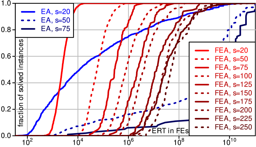
Figure 10: The ERT-ECDF curves for the SATLib instances: the fraction of instances of a given dimension $s$ solved over their empirically determined expected runtime.

We now plot the Empirical Cumulative Distribution Function (ECDF [29]) over the estimated ERT in Figure 10. Normally, the ECDF shows the fraction of runs that could solve their corresponding problem instance over time. However, we want to illustrate which algorithm can solve which fraction of the instances until which (empirically determined expected) time. For a given dimension $s$, we therefore compute the ERT for each of the corresponding instances based on the conducted runs.

It seems that SATLib contains some instances that the $\mbox{(1+1)-\mbox{{EA}}}_{>0}$ can solve quickly, but on many instances it is slow or fails often. The ERT of the instance of dimension $s=250$ hardest for the $\mbox{(1+1)-\mbox{{FEA}}}_{>0}$ is only 38% higher than the ERT of the scale-20 instance hardest for the $\mbox{(1+1)-\mbox{{EA}}}_{>0}$. Due to the drop in success rate, the behavior of the $\mbox{(1+1)-\mbox{{EA}}}_{>0}$ is already very unstable at dimensions 50 and 75. This does not happen for the $\mbox{(1+1)-\mbox{{FEA}}}_{>0}$ at any of the tested dimensions.

In summary, the (1+1)-FEA very significantly outperforms the (1+1)-EA on a practically-relevant task, which goes beyond the scope of toy problems.

IV-J Job Shop Scheduling Problems (JSSP)

With the MaxSat, we have investigated an important $\mathcal{NP}$-hard problem. While exhibiting interesting features, the $\mbox{(1+1)-\mbox{{FEA}}}_{>0}$ algorithm we applied is not competitive to the state-of-the-art even two decades ago [60]. We now want to investigate if FFA can be helpful when the base algorithm is already performing well and we will do so on an entirely different domain.

In a job shop scheduling problem (JSSP) [61] without preemption, there are $M$ machines and $N$ jobs. Each job must be processed by all machines in a job-specific sequence and has, for each machine, a specific processing time. The goal is to find assignments of jobs to machines that result in an overall shortest makespan, i.e., the schedule which can complete all the jobs the fastest. The JSSP is $\mathcal{NP}$-hard [61]. The objective values are positive integers since the processing times are integers. We obtain an upper bound $U\!B$ needed for FFA as the sum of all processing times of all sub-jobs. We use the JSSP as educational example in [62], where we discuss all of the following components (except FFA) in great detail.

A solution for the JSSP is encoded as permutation with repetition, as integer strings where each of the $N$ job IDs occurs exactly $M$ times [63]. Such an integer string $x$ is processed from front to end. When encountering job $i$, we know to which machine $j$ it needs to go next based on the job-specific machine sequence and on how often we already saw $i$ in $x$ before. We can start it on $j$ at a time which is the maximum of 1) when the previous sub-job assigned to $j$ will finish and 2) when the previous sub-job of $i$ completes on its corresponding machine.

We develop a memetic algorithm [64] which retains the $\mbox{$\mu$}=16$ best candidate solutions in its population and generates $\mbox{$\lambda$}=16$ new strings in each step via recombination. Recombination proceeds similar to the solution decoding, but reads unprocessed sub-jobs iteratively from two parent strings (between which it randomly switches) and writes them to an offspring, while marking each processed sub-job in both parents as processed [62]. The $\lambda$ new strings each are refined with ten steps of a local search which, in each step, scans the single-swap neighborhood of the string in random order until it finds a makespan-improving move and applies it (or stops if none can be found).

The two algorithms we investigate differ only in what they do once this step is completed: The first, MA, now applies selection based on the objective values. In the FMA, on the other hand, the FFA table $H$ is updated by increasing the frequency counter of the corresponding objective value of each of the $\mbox{$\mu$}+\mbox{$\lambda$}$ solutions in the joint parent-offspring population. Selection chooses the $\mu$ solutions with the lowest frequency fitness value. FMA still uses the objective function $f$ in the local search and to break ties in FFA. It is therefore not invariant under bijections of $f$.

Our goal this time is to achieve the best possible result within five minutes of runtime on an Intel Core i7 8700 CPU with 3.2 GHz and 16 GiB RAM under Java OpenJDK 13 on Ubuntu 19.04. This is very different from the previous goals of solving the problems to optimality. We conduct $r=11$ runs each on 82 well-known JSSP instances from the OR-Library [65, 66], namely the sets abz*, ft*, la*, orb*, swv*, and yn*, where all processing times are integers.

TABLE III: Best, median, mean, and standard deviation of results from 11 runs of MA and FMA; bold: better value, green shading: best known solutions (BKS) reached.

0pt MA FMA inst BKS+ref best med mean sd best med mean sd abz5 1234 [67] 1239 1244 1244.1 4.9 1234 1234 1236.2 2.5 abz6 943 [67] 947 948 949.0 3.9 943 943 943.4 1.2 abz7 656 [68] 679 693 694.7 10.8 685 691 693.1 5.5 abz8 665 [68] 698 709 713.2 12.4 688 706 705.9 8.2 abz9 678 [69] 724 737 736.2 6.7 714 727 725.6 6.7 ft06 55 [70] 55 55 55.0 0.0 55 55 55.0 0.0 ft10 930 [70] 937 949 948.2 7.6 930 930 933.9 6.1 ft20 1165 [70] 1173 1178 1177.9 1.8 1165 1178 1176.4 4.1 la01 666 [67] 666 666 666.0 0.0 666 666 666.0 0.0 la02 655 [67] 655 655 655.0 0.0 655 655 655.0 0.0 la03 597 [67] 597 597 599.2 4.9 597 597 597.0 0.0 la04 590 [67] 590 590 590.0 0.0 590 590 590.0 0.0 la05 593 [67] 593 593 593.0 0.0 593 593 593.0 0.0 la06 926 [67] 926 926 926.0 0.0 926 926 926.0 0.0 la07 890 [67] 890 890 890.0 0.0 890 890 890.0 0.0 la08 863 [67] 863 863 863.0 0.0 863 863 863.0 0.0 la09 951 [67] 951 951 951.0 0.0 951 951 951.0 0.0 la10 958 [67] 958 958 958.0 0.0 958 958 958.0 0.0 la11 1222 [67] 1222 1222 1222.0 0.0 1222 1222 1222.0 0.0 la12 1039 [67] 1039 1039 1039.0 0.0 1039 1039 1039.0 0.0 la13 1150 [67] 1150 1150 1150.0 0.0 1150 1150 1150.0 0.0 la14 1292 [67] 1292 1292 1292.0 0.0 1292 1292 1292.0 0.0 la15 1207 [67] 1207 1207 1207.0 0.0 1207 1207 1207.0 0.0 la16 945 [67] 946 946 959.4 17.5 945 946 945.9 0.3 la17 784 [67] 784 787 787.5 3.0 784 784 784.0 0.0 la18 848 [67] 848 848 850.0 4.5 848 848 848.0 0.0 la19 842 [67] 842 852 853.4 8.7 842 842 842.9 3.0 la20 902 [67] 907 907 907.8 1.8 902 907 906.5 1.5 la21 1046 [71] 1056 1068 1067.8 7.5 1047 1053 1052.5 2.7 la22 927 [67] 935 941 941.3 8.0 930 935 934.5 1.9 la23 1032 [67] 1032 1032 1032.0 0.0 1032 1032 1032.0 0.0 la24 935 [67] 941 964 960.2 11.7 941 946 945.6 3.2 la25 977 [67] 986 998 1002.3 14.8 984 986 986.7 3.1 la26 1218 [67] 1218 1218 1222.4 11.6 1218 1218 1218.0 0.0 la27 1235 [71] 1252 1269 1268.3 8.3 1248 1264 1264.0 6.7 la28 1216 [67] 1225 1232 1238.7 14.5 1216 1225 1228.1 8.8 la29 1152 [68] 1199 1222 1224.2 18.9 1191 1219 1212.6 13.0 la30 1355 [67] 1355 1355 1355.0 0.0 1355 1355 1355.0 0.0 la31 1784 [67] 1784 1784 1784.0 0.0 1784 1784 1784.0 0.0 la32 1850 [67] 1850 1850 1850.0 0.0 1850 1850 1850.0 0.0 la33 1719 [67] 1719 1719 1719.0 0.0 1719 1719 1719.0 0.0 la34 1721 [67] 1721 1721 1721.0 0.0 1721 1721 1721.0 0.0 la35 1888 [67] 1888 1888 1888.0 0.0 1888 1888 1888.0 0.0 la36 1268 [67] 1295 1301 1307.7 15.7 1281 1297 1297.5 9.8 la37 1397 [67] 1446 1467 1462.3 13.5 1432 1446 1442.5 6.3 la38 1196 [72] 1251 1263 1262.9 13.5 1239 1240 1244.6 8.7 la39 1233 [67] 1251 1256 1267.0 20.5 1248 1250 1250.0 1.2 la40 1222 [67] 1241 1264 1262.1 14.0 1233 1247 1247.3 7.7 orb01 1059 [67] 1059 1104 1099.2 17.5 1071 1071 1075.4 5.6 orb02 888 [67] 890 919 909.0 14.3 889 889 889.0 0.0 orb03 1005 [67] 1026 1058 1060.5 27.8 1005 1022 1019.5 7.4 orb04 1005 [67] 1005 1028 1024.3 14.0 1005 1011 1010.0 2.2 orb05 887 [67] 890 905 913.8 18.1 887 890 890.2 2.4 orb06 1010 [73] 1013 1031 1031.0 8.6 1013 1013 1017.8 6.0 orb07 397 [68] 397 397 401.7 7.4 397 397 397.1 0.3 orb08 899 [73] 914 944 941.3 16.5 899 899 902.0 5.4 orb09 934 [73] 939 945 947.9 7.2 934 939 937.9 3.4 orb10 944 [73] 944 946 957.3 15.9 944 944 944.0 0.0 swv01 1407 [68] 1476 1517 1524.1 35.1 1447 1474 1483.3 20.9 swv02 1475 [68] 1550 1585 1582.8 20.9 1525 1548 1549.1 15.5 swv03 1398 [68] 1500 1530 1533.3 28.8 1489 1512 1513.1 15.1 swv04 1464 [74][75] 1580 1615 1624.1 30.6 1564 1578 1586.5 22.3 swv05 1424 [68] 1517 1575 1585.3 49.8 1523 1554 1556.0 25.8 swv06 1671 [75] 1859 1903 1909.2 44.0 1824 1864 1862.7 27.8 swv07 1594 [76] 1766 1814 1816.1 26.4 1705 1755 1753.3 24.5 swv08 1752 [75] 1940 1992 1989.9 38.0 1930 1946 1946.4 13.9 swv09 1655 [75] 1820 1871 1877.9 51.8 1805 1844 1844.8 19.3 swv10 1743 [76] 1909 1956 1974.5 44.7 1904 1936 1931.4 15.4 swv11 2983 [77] 3439 3506 3506.1 52.6 3495 3574 3583.5 62.6 swv12 2977 [78] 3478 3594 3594.4 56.3 3511 3605 3622.1 66.3 swv13 3104 [68] 3543 3679 3686.5 81.1 3578 3664 3677.2 78.6 swv14 2968 [68] 3358 3455 3444.4 60.4 3369 3454 3452.9 69.1 swv15 2885 [78] 3361 3500 3490.6 89.5 3356 3529 3524.1 98.5 swv16 2924 [68] 2924 2924 2924.0 0.0 2924 2924 2924.0 0.0 swv17 2794 [68] 2794 2794 2794.0 0.0 2794 2794 2794.0 0.0 swv18 2852 [68] 2852 2852 2852.0 0.0 2852 2852 2852.0 0.0 swv19 2843 [68] 2843 2843 2843.0 0.0 2843 2843 2843.0 0.0 swv20 2823 [68] 2823 2823 2823.0 0.0 2823 2823 2823.0 0.0 yn1 884 [69] 921 934 936.2 11.7 909 931 931.5 10.7 yn2 904 [76] 953 962 964.0 7.5 937 954 952.4 9.8 yn3 892 [77] 929 951 951.9 16.1 913 938 938.6 12.0 yn4 968 [68] 1022 1046 1048.9 20.0 1024 1041 1041.9 9.0

From Table III, we can find that MA can already discover the best known solution (BKS) on 36 instances at least once and always on 27. FMA, however, can do so 46 and 32 times, respectively. FMA has better best, median, and mean results 37, 45, and 51 times, respectively, while the same is true for the MA only 8, 3, and 4 times. In other words, on 93% of the instances that are not already always solved to optimality by MA, FMA has a better mean result. The mean (median) result of FMA is better than the best result of MA in 17 (13) instances, while the opposite is never true. FMA has a smaller standard deviation in 48 cases, MA only in 4. We apply the two-sided Welch’s t-test to the results on the 49 instances where the algorithms have different mean results with non-zero standard deviations. FMA performs significantly better than MA on 25 of them at a significance level of $\alpha=0.01$. Such high significance is a very strong result at only 11 runs. The opposite is true only on swv11, even if we set $\alpha=0.1$.

Neither MA nor FMA can outperform the state-of-the-art on the JSSP, but they are not very far off, at least if we consider result quality only: The basic MA obtains better best (mean) results than the GWO proposed in [79] (2018) in 16 (21) of the 39 instances for which results are provided, while the opposite is never (once) true. While the HFSAQ [80] (2016) has better mean (best) result quality in 23 (12) of 48 comparable cases, FMA scores even in the rest, while having better mean solution quality on 4 instances. It also 13 times achieves better mean makespans (28 times worse ones) on the 63 common instances compared to the HIMGA [81] (2015), while its best solution is never better. On instances swv16 to swv20, which can be solved to the BKS by both MA and FMA, budgets of more than 16 min were used in [68] to find said BKSes. Still, the FMA is worse than, e.g., the algorithms in [82] (2016) and [75] (2015) on every common instance where it does not find the BKS.

In summary, we find that even in a more complicated setup based on an algorithm that already does not perform badly in comparison to recent publications, FFA can lead to a significant performance improvement. This does not mean that other diversity improvement strategies, e.g., those from Section III, could not have improved the performance of the MA as well or even better. Still, together with the results on the MaxSat problems in Section IV-I and those in our earlier papers on FFA on domains such as Genetic Programming [2, 1], this adds evidence to the idea that FFA may not just be of purely academic interest.

V Conclusions

In this paper, we plugged Frequency Fitness Assignment (FFA) into the most basic evolutionary algorithm, the (1+1)-EA, and applied the resulting (1+1)-FEA to several problems defined over bit strings of dimension $s$. On the one hand, we found that the (1+1)-FEA is slower than the (1+1)-EA on the OneMax, LeadingOnes, and Plateau functions. In our experiments with these problems, it seems to increase the mean runtime needed to discover the global optimum by a factor no worse than linear in the number of objective values or in $s$. On the other hand, FFA can seemingly decrease the mean runtime on the Trap, Jump, and TwoMax problems from exponential to the scale of $s^{2}\ln{s}$. On the MaxSat problem and on the W-Model benchmark, the (1+1)-FEA very significantly outperforms the (1+1)-EA.

These results are surprising when considering the nature of FFA – being invariant under bijective transformations of the objective function, i.e., possessing the strongest invariance property known to us. FFA never compares objective values directly. An algorithm applying only FFA would exhibit the same performance on the objective function $f$ as on $g\circ f$, where $g$ could be an arbitrary encryption method (which we simulate by setting $g$ to the Md5 checksum routine in Section IV-G).

This realization is baffling. Two central assumptions of black-box optimization are that following a trail of improving objective values tends to be a good idea and that “nice” optimization problems should exhibit causality, i.e., small changes to a solution should lead to small changes in its objective value. Under FFA, neither assumption is used. As a result, properties such as causality, ruggedness, or deceptiveness of a fitness landscape may have little impact on the algorithm performance. Interestingly, this does seemingly not necessarily come at a high cost in terms of runtime. Instead of the cost of the invariance, the limitation of the method seems to be that it requires objective functions that can be discretized and do not take on too many different values.

We finally showed that FFA can be combined with “normal” optimization and plugged into more complex algorithms. We inserted it into the selection step of a memetic algorithm whose local search proceeds without FFA and works directly on the objective values. Here, an FFA variant purely works as population diversity enhancement mechanism and can improve the result quality that the algorithm produces on the JSSP within a budget of five minutes. Notably, while this algorithm does not belong to the state-of-the-art on the JSSP, it seems to be relatively close to it. Together with our results on the MaxSat problem, this means that FFA might even be helpful in cases bordering to practical relevance.

There are several interesting avenues for future work. First, we want to also plug FFA into other EAs, such as those in [8]. Second, a theoretical analysis of the properties of FFA could be both interesting and challenging, also from the perspective of black-box complexity. Third, using FFA is the only approach known to us that can solve encrypted optimization problems. This could open new types of applications in operations research, machine learning, and artificial intelligence. Fourth, on problems FFA leads to a slowdown. The question whether this slowdown is proportional to the problem dimension or to the number of possible different objective values deserves an investigation.

Finally, it may be possible to adapt ideas from the research on multi-armed bandits to implement an FFA-like approach: We envisage an Upper Confidence Bound [83]-like algorithm, where one solution per encountered objective value is preserved and treated as bandit arm. Playing an arm would mean to use the solution as input to mutation and the reward could be 1 if the offspring has a new objective value.

Thomas Weise obtained his Ph.D. in Computer Science from the University of Kassel (Kassel, Germany) in 2009. He then joined the University of Science and Technology of China (Hefei, Anhui, China), first as PostDoc, later as Associate Professor. In 2016, he moved to Hefei University (in Hefei) as Full Professor to found the Institute of Applied Optimization (IAO) at the School of Artificial Intelligence and Big Data. His research interests include metaheuristic optimization and algorithm benchmarking. He was awarded the title Hefei Specially Recruited Foreign Expert of the city Hefei in Anhui, China in 2019.

Zhize Wu obtained his Bachelor from the Anhui Normal University (Wuhu, Anhui, China) in 2012 and his Ph.D. in Computer Science from the University of Science and Technology of China (Hefei, Anhui, China) in 2017. He then joined the Institute of Applied Optimization (IAO) of the School of Artificial Intelligence and Big Data at Hefei University as Lecturer. His research interest include image processing, neural networks, deep learning, machine learning in general, and algorithm benchmarking.

Xinlu Li received his Bachelor from the Fuyang Normal University (Fuyang, Anhui, China) in 2002, his M.Sc. degree in Computer Science from Anhui University (Hefei, Anhui, China) in 2009, and his Ph.D. degree in Computer Science from the TU Dublin (Dublin, Ireland) in 2019. His career at Hefei University started as Lecturer in 2009, Senior Lecturer in 2012, in 2018 he joined the Institute of Applied Optimization (IAO), and in 2019 he became Associate Researcher. From 2014 to 2018, he was Teaching Assistant in the School of Computing of TU Dublin. His research interest include Swarm Intelligence and optimization, algorithms which he applies to energy efficient routing protocol design for large-scale Wireless Sensor Networks.

Yan Chen received his Bachelor from the Anhui University of Science and Technology (Huai’nan, Anhui, China) in 2011, his M.Sc. degree from the China University of Mining and Technology (Xuzhou, Jiangsu, China) in 2014, and his doctorate from the TU Dortmund (Dortmund, Germany) in 2019. There, he studied spatial information management and modeling as a member of the Spatial Information Management and Modelling Department of the School of Spatial Planning. He joined the Institute of Applied Optimization (IAO) of the School of Artificial Intelligence and Big Data at Hefei University as Lecturer in 2019. His research interests include hydrological modeling, Geographic Information System, Remote Sensing, and Sponge City/Smart City applications, as well as deep learning and optimization algorithms.

References

- [1] T. Weise, M. Wan, K. Tang, P. Wang, A. Devert, and X. Yao, “Frequency fitness assignment,” IEEE Transactions on Evolutionary Computation, vol. 18, no. 2, pp. 226–243, 2014.
- [2] T. Weise, M. Wan, K. Tang, and X. Yao, “Evolving exact integer algorithms with genetic programming,” in IEEE Congress on Evolutionary Computation (CEC’14). Los Alamitos, CA, USA: IEEE, 2014, pp. 1816–1823.
- [3] Y. Ollivier, L. Arnold, A. Auger, and N. Hansen, “Information-geometric optimization algorithms: A unifying picture via invariance principles,” Journal of Machine Learning Research, vol. 18, pp. 18:1–18:65, 2017.
- [4] L. D. Whitley, “The GENITOR algorithm and selection pressure: Why rank-based allocation of reproductive trials is best,” in 3rd Intl. Conf. on Genetic Algorithms (ICGA’89). San Francisco, CA, USA: Morgan Kaufmann Publishers Inc., 1989, pp. 116–121.
- [5] N. Hansen, R. Ros, N. Mauny, M. Schoenauer, and A. Auger, “Impacts of invariance in search: When CMA-ES and PSO face ill-conditioned and non-separable problems,” Applied Soft Computing, vol. 11, no. 8, pp. 5755–5769, 2011.
- [6] T. Bäck, D. B. Fogel, and Z. Michalewicz, Eds., Handbook of Evolutionary Computation. New York, USA: Oxford University Press, 1997.
- [7] S. Droste, T. Jansen, and I. Wegener, “On the analysis of the evolutionary algorithm,” Theor. Comput. Sci., vol. 276, no. 1-2, pp. 51–81, 2002.
- [8] E. Carvalho Pinto and C. Doerr, “Towards a more practice-aware runtime analysis of evolutionary algorithms,” 2017, arXiv:1812.00493v1 [cs.NE] 3 Dec 2018. [Online]. Available: http://arxiv.org/pdf/1812.00493.pdf
- [9] H. Mühlenbein, “How genetic algorithms really work: Mutation and hillclimbing,” in Parallel Problem Solving from Nature 2 (PPSN-II). Elsevier, 1992, pp. 15–26.
- [10] P. K. Lehre and P. S. Oliveto, “Theoretical analysis of stochastic search algorithms,” in Handbook of Heuristics, R. Martí, P. Panos, and M. G. C. Resende, Eds. Springer, 2018, pp. 1–36.
- [11] T. H. Cormen, C. E. Leiserson, R. L. Rivest, and C. Stein, Introduction to Algorithms, 3rd ed. Cambridge, MA, USA: Massachusetts Institute of Technology, 2009.
- [12] D. E. Goldberg and J. T. Richardson, “Genetic algorithms with sharing for multimodal function optimization,” in 2nd Intl. Conf. on Genetic Algorithms and their Applications (ICGA’87). Mahwah, NJ, USA: Lawrence Erlbaum Associates, Inc., 1987, pp. 41–49.
- [13] A. Pétrowski, “A clearing procedure as a niching method for genetic algorithms,” in IEEE Intl. Conf. on Evolutionary Computation (CEC’96). Los Alamitos, CA, USA: IEEE, 1996, pp. 798–803.
- [14] T. Friedrich, P. S. Oliveto, D. Sudholt, and C. Witt, “Analysis of diversity-preserving mechanisms for global exploration,” Evolutionary Computation, vol. 17, no. 4, pp. 455–476, 2009.
- [15] F. W. Glover, É. D. Taillard, and D. de Werra, “A user’s guide to tabu search,” Annals of Operations Research, vol. 41, no. 1, pp. 3–28, 1993.
- [16] M. Hutter, “Fitness uniform selection to preserve genetic diversity,” in IEEE Congress on Evolutionary Computation (CEC’02), vol. 1-2. Los Alamitos, CA, USA: IEEE, 2002, pp. 783–788.
- [17] M. Hutter and S. Legg, “Fitness uniform optimization,” IEEE Transactions on Evolutionary Computation, vol. 10, no. 5, pp. 568–589, 2006.
- [18] D. Corus, P. S. Oliveto, and D. Yazdani, “When hypermutations and ageing enable artificial immune systems to outperform evolutionary algorithms,” Theor. Comput. Sci., vol. 832, pp. 166–185, 2020.
- [19] ——, “Fast artificial immune systems,” in Proc. of the 15th Intl. Conf. on Parallel Problem Solving from Nature (PPSN XV), Part II. Springer, 2018, pp. 67–78.
- [20] ——, “Artificial immune systems can find arbitrarily good approximations for the NP-hard number partitioning problem,” Artif. Intell., vol. 274, pp. 180–196, 2019.
- [21] A. Ghosh, S. Tsutsui, and H. Tanaka, “Individual aging in genetic algorithms,” in Proceedings of the Australian New Zealand Conference on Intelligent Information Systems (ANZIIS’96). IEEE, 1996, pp. 276–279.
- [22] D. Gravina, A. Liapis, and G. N. Yannakakis, “Quality diversity through surprise,” IEEE Transactions on Evolutionary Computation, vol. 23, no. 4, pp. 603–616, 2019.
- [23] A. Cully and Y. Demiris, “Quality and diversity optimization: A unifying modular framework,” IEEE Transactions on Evolutionary Computation, vol. 22, no. 2, pp. 245–259, 2018.
- [24] J. K. Pugh, L. B. Soros, and K. O. Stanley, “Quality diversity: A new frontier for evolutionary computation,” Frontiers in Robotics and AI, vol. 2016, 2016.
- [25] J. Lehman and K. O. Stanley, “Abandoning objectives: Evolution through the search for novelty alone,” Evolutionary Computation, vol. 19, no. 2, pp. 189–223, 2011.
- [26] ——, “Evolving a diversity of virtual creatures through novelty search and local competition,” in 13th Annual Genetic and Evolutionary Computation Conf. (GECCO’11). ACM, 2011, pp. 211–218.
- [27] J. Mouret and J. Clune, “Illuminating search spaces by mapping elites,” 2015, arXiv:1504.04909v1 [cs.AI] 20 Apr 2015. [Online]. Available: http://arxiv.org/abs/1504.04909
- [28] D. Gravina, A. Liapis, and G. N. Yannakakis, “Surprise search: Beyond objectives and novelty,” in Genetic and Evolutionary Computation Conf. (GECCO’16). ACM, 2016, pp. 677–684.
- [29] N. Hansen, A. Auger, S. Finck, and R. Ros, “Real-parameter black-box optimization benchmarking: Experimental setup,” Université Paris Sud, INRIA Futurs, Équipe TAO, Orsay, France, Tech. Rep., 2012. [Online]. Available: http://coco.lri.fr/BBOB-downloads/download11.05/bbobdocexperiment.pdf
- [30] T. Weise, Z. Wu, X. Li, and Y. Chen, The Experimental Data for the Study “Frequency Fitness Assignment: Making Optimization Algorithms Invariant under Bijective Transformations of the Objective Function Value”. Genève, Switzerland: CERN, 2020. [Online]. Available: http://doi.org/10.5281/zenodo.3899474
- [31] P. Erdős and A. Rényi, “On two problems of information theory,” Publ. Math. Inst. Hung. Acad. Sci., Ser. A, vol. 8, pp. 229–243, 1963.
- [32] S. Droste, T. Jansen, and I. Wegener, “Upper and lower bounds for randomized search heuristics in black-box optimization,” Theory of Computing Systems, vol. 39, no. 4, pp. 525–544, 2006.
- [33] H. Hwang, A. Panholzer, N. Rolin, T. Tsai, and W. Chen, “Probabilistic analysis of the (1+1)-evolutionary algorithm,” Evolutionary Computation, vol. 26, no. 2, 2018.
- [34] B. Doerr, “Analyzing randomized search heuristics via stochastic domination,” Theor. Comput. Sci., vol. 773, pp. 115–137, 2019.
- [35] G. Rudolph, Convergence Properties of Evolutionary Algorithms. Hamburg, Germany: Verlag Dr. Kovač, 1997.
- [36] P. Afshani, M. Agrawal, B. Doerr, K. G. Larsen, K. Mehlhorn, and C. Winzen, “The query complexity of finding a hidden permutation,” in Space-Efficient Data Structures, Streams, and Algorithms – Papers in Honor of J. Ian Munro on the Occasion of His 66th Birthday. Springer, 2013, ch. 1, pp. 1–11.
- [37] S. Böttcher, B. Doerr, and F. Neumann, “Optimal fixed and adaptive mutation rates for the leadingones problem,” in 11th Intl. Conf. on Parallel Problem Solving from Nature (PPSN XI), Part I. Springer, 2010, pp. 1–10.
- [38] D. Sudholt, “A new method for lower bounds on the running time of evolutionary algorithms,” IEEE Transactions on Evolutionary Computation, vol. 17, no. 3, pp. 418–435, 2013.
- [39] T. Friedrich, F. Quinzan, and M. Wagner, “Escaping large deceptive basins of attraction with heavy-tailed mutation operators,” in Genetic and Evolutionary Computation Conf. (GECCO’18). ACM, 2018, pp. 293–300.
- [40] C. Van Hoyweghen, D. E. Goldberg, and B. Naudts, “From Twomax to the ising model: Easy and hard symmetrical problems,” in Genetic and Evolutionary Computation Conf. (GECCO’02). Morgan Kaufmann, 2002, pp. 626–633.
- [41] B. Doerr, C. Doerr, and T. Kötzing, “Unbiased black-box complexities of jump functions,” Evolutionary Computation, vol. 23, no. 4, pp. 641–670, 2015.
- [42] B. Doerr, H. P. Le, R. Makhmara, and T. D. Nguyen, “Fast genetic algorithms,” in Proc. of the Genetic and Evolutionary Computation Conference (GECCO’17). ACM, 2017, pp. 777–784.
- [43] B. Doerr, “A tight runtime analysis for the cGA on jump functions: EDAs can cross fitness valleys at no extra cost,” in Proc. of the Genetic and Evolutionary Computation Conference (GECCO’19). ACM, 2019, pp. 1488–1496.
- [44] ——, “An exponential lower bound for the runtime of the cGA on jump functions,” 2019, arXiv:1904.08415v2 [cs.NE] 25 Jun 2019. [Online]. Available: http://arxiv.org/abs/1904.08415
- [45] S. Nijssen and T. Bäck, “An analysis of the behavior of simplified evolutionary algorithms on trap functions,” IEEE Transactions on Evolutionary Computation, vol. 7, no. 1, pp. 11–22, 2003.
- [46] D. Antipov and B. Doerr, “Precise runtime analysis for plateaus,” in 15th Intl. Conf. on Parallel Problem Solving from Nature PPSN XV, Part II. Springer, 2018, pp. 117–128.
- [47] R. L. Rivest, “The MD5 message-digest algorithm,” Network Working Group, RFC, 1992. [Online]. Available: http://tools.ietf.org/html/rfc1321
- [48] T. Weise and Z. Wu, “Difficult features of combinatorial optimization problems and the tunable W-Model benchmark problem for simulating them,” in Companion Material Genetic and Evolutionary Computation Conf. (GECCO’18). ACM, 2018, pp. 1769–1776.
- [49] T. Weise, “The W-Model, a tunable black-box discrete optimization benchmarking (BB-DOB) problem, implemented for the BB-DOB@GECCO workshop,” 2018. [Online]. Available: http://github.com/thomasWeise/BBDOB_W_Model
- [50] T. Weise, S. Niemczyk, H. Skubch, R. Reichle, and K. Geihs, “A tunable model for multi-objective, epistatic, rugged, and neutral fitness landscapes,” in 10th Annual Conf. on Genetic and Evolutionary Computation Conf. (GECCO’08). New York, USA: ACM Press, 2008, pp. 795–802.
- [51] T. Weise, Y. Chen, X. Li, and Z. Wu, “Selecting a diverse set of benchmark instances from a tunable model problem for black-box discrete optimization algorithms,” Applied Soft Computing, vol. 92, p. 106269, 2019.
- [52] T. Weise, Results for Several Simple Algorithms on the W-Model for Black-Box Discrete Optimization Benchmarking. Genève, Switzerland: CERN, 2018.
- [53] M. R. Garey and D. S. Johnson, Computers and Intractability: A Guide to the Theory of -Completeness. New York, USA: W. H. Freeman and Company, 1979.
- [54] H. H. Hoos and T. Stützle, Stochastic Local Search: Foundations and Applications. San Francisco, CA, USA: Morgan Kaufmann Publishers Inc., 2005.
- [55] S. B. Rana and L. D. Whitley, “Genetic algorithm behavior in the MAXSAT domain,” in 5th Intl. Conf. on Parallel Problem Solving from Nature (PPSN V). Springer, 1998, pp. 785–794.
- [56] H. H. Hoos and T. Stützle, “SATLIB: An online resource for research on SAT,” in SAT2000 – Highlights of Satisfiability Research in the Year 2000. Amsterdam, The Netherlands: IOS Press, 2000, pp. 283–292.
- [57] B. Doerr, F. Neumann, and A. M. Sutton, “Time complexity analysis of evolutionary algorithms on random satisfiable k-CNF formulas,” Algorithmica, vol. 78, no. 2, pp. 561–586, 2017.
- [58] ——, “Improved runtime bounds for the (1+1) EA on random 3-CNF formulas based on fitness-distance correlation,” in Genetic and Evolutionary Computation Conf. (GECCO’15). ACM, 2015, pp. 1415–1422.
- [59] C. P. Gomes, H. A. Kautz, A. Sabharwal, and B. Selman, “Satisfiability solvers,” in Handbook of Knowledge Representation. Elsevier, 2008, pp. 89–134.
- [60] H. H. Hoos and T. Stützle, “Local search algorithms for SAT: An empirical evaluation,” Journal of Automated Reasoning, vol. 24, no. 4, pp. 421–481, 2000.
- [61] E. L. Lawler, J. K. Lenstra, A. H. G. Rinnooy Kan, and D. B. Shmoys, “Sequencing and scheduling: Algorithms and complexity,” in Handbook of Operations Research and Management Science. Amsterdam, The Netherlands: North-Holland Scientific Publishers Ltd., 1993, vol. IV: Production Planning and Inventory, ch. 9, pp. 445–522.
- [62] T. Weise, An Introduction to Optimization Algorithms. Hefei, Anhui, China: Institute of Applied Optimization (IAO), School of Artificial Intelligence and Big Data, Hefei University, 2018–2019.
- [63] M. Gen, Y. Tsujimura, and E. Kubota, “Solving job-shop scheduling problems by genetic algorithm,” in Humans, Information and Technology: 1994 IEEE Intl. Conf. on Systems, Man and Cybernetics, vol. 2. IEEE, 1994.
- [64] F. Neri, C. Cotta, and P. Moscato, Eds., Handbook of Memetic Algorithms. Berlin/Heidelberg: Springer, 2012.
- [65] J. E. Beasley, “OR-Library: Distributing test problems by electronic mail,” The Journal of the Operational Research Society, vol. 41, pp. 1069–1072, 1990.
- [66] ——, “OR-Library: Job shop scheduling,” 1990. [Online]. Available: http://people.brunel.ac.uk/~mastjjb/jeb/orlib/jobshopinfo.html
- [67] D. L. Applegate and W. J. Cook, “A computational study of the job-shop scheduling problem,” ORSA Journal on Computing, vol. 3, no. 2, pp. 149–156, 1991.
- [68] A. Henning, “Praktische Job-Shop Scheduling-Probleme,” Ph.D. dissertation, Friedrich-Schiller-Universität Jena, Jena, Germany, 2002.
- [69] C. Zhang, X. Shao, Y. Rao, and H. Qiu, “Some new results on tabu search algorithm applied to the job-shop scheduling problem,” in Tabu Search. London, UK: IntechOpen, 2008.
- [70] J. Carlier and É. Pinson, “An algorithm for solving the job-shop problem,” Management Science, vol. 35, no. 2, pp. 164–176, 1989, jstor: 2631909.
- [71] T. Yamada and R. Nakano, “Genetic algorithms for job-shop scheduling problems,” in Modern Heuristic for Decision Support. UNICOM seminar, 1997, pp. 67–81.
- [72] E. Nowicki and C. Smutnicki, “A fast taboo search algorithm for the job shop problem,” Management Science, vol. 42, no. 6, pp. 783–938, 1996, jstor: 2634595.
- [73] E. Balas and A. Vazacopoulos, “Guided local search with shifting bottleneck for job shop scheduling,” Management Science, vol. 44, no. 2, pp. 262–275, 1998.
- [74] P. Vilím, P. Laborie, and P. Shaw, “Failure-directed search for constraint-based scheduling,” in 12th Intl. Conf. on AI and OR Techniques in Constriant Programming for Combinatorial Optimization Problems (CPAIOR’2015). Cham, Switzerland: Springer, 2015, pp. 437–453.
- [75] ——, “Failure-directed search for constraint-based scheduling – detailed experimental results,” 2015, the detailed experimental results of the paper [74]. [Online]. Available: http://vilim.eu/petr/cpaior2015-results.pdf
- [76] J. F. Gonçalves and M. G. C. Resende, “An extended Akers graphical method with a biased random-key genetic algorithm for job-shop scheduling,” International Transactions on Operational Research, vol. 21, no. 2, pp. 215–246, 2014.
- [77] E. Nowicki and C. Smutnicki, “An advanced taboo search algorithm for the job shop problem,” Journal of Scheduling, vol. 8, no. 2, pp. 145–159, 2005.
- [78] B. Peng, Z. Lü, and T. C. E. Cheng, “A tabu search/path relinking algorithm to solve the job shop scheduling problem,” Computers & Operations Research, vol. 53, pp. 154–164, 2015.
- [79] T. Jiang and C. Zhang, “Application of grey wolf optimization for solving combinatorial problems: Job shop and flexible job shop scheduling cases,” IEEE Access, vol. 6, pp. 26 231–26 240, 2018.
- [80] K. Akram, K. Kamal, and A. Zeb, “Fast simulated annealing hybridized with quenching for solving job shop scheduling problem,” Applied Soft Computing, vol. 49, pp. 510–523, 2016.
- [81] M. Kurdi, “A new hybrid island model genetic algorithm for job shop scheduling problem,” Computers & Industrial Engineering, vol. 88, pp. 273–283, 2015.
- [82] T. C. E. Cheng, B. Peng, and Z. Lü, “A hybrid evolutionary algorithm to solve the job shop scheduling problem,” Annals of Operations Research, vol. 242, no. 2, pp. 223–237, 2016.
- [83] P. Auer, N. Cesa-Bianchi, and P. Fischer, “Finite-time analysis of the multiarmed bandit problem,” Machine Learning, vol. 47, no. 2-3, pp. 235–256, 2002.