A time-optimal feedback control for a particular case of the game of two cars

Abstract

In this paper, a computationally efficient time-optimal feedback solution to the game of two cars, for the case where the pursuer is faster and more agile than the evader, is presented. The concept of continuous subsets of the reachable set is introduced to characterize the time-optimal pursuit-evasion game under feedback strategies. Using these subsets it is shown that, if initially the pursuer is distant enough from the evader, then the feedback saddle point strategies for both the pursuer and the evader are coincident with one of the common tangents from the minimum radius turning circles of the pursuer to the minimum radius turning circles of the evader. Using geometry, four feasible tangents are identified and the feedback $\min-\max$ strategy for the pursuer and the $\max-\min$ strategy for the evader are derived by solving a $2\times 2$ matrix game at each instant. Insignificant computational effort is involved in evaluating the pursuer and evader inputs using the proposed feedback control law and hence it is suitable for real-time implementation.

I Introduction

Pursuit evasion is a differential game between two antagonistic agents called the pursuer and the evader. The pursuer aims to capture the evader in minimum time whereas evader aims to avoid capture for as long as possible. The problem of time optimal pursuit evasion for two Dubins vehicles or the game of two cars was first introduced by Issacs in [1]. A Dubins vehicle consists of a point moving in a plane with a given maximum forward velocity and a minimum turning radius. In [1] the pursuer is considered superior to the evader and the regions of capture are characterized by backward integration of Issacs equation for the game in reduced state-space. This results in the so called retrogressive path equations. The optimal control law synthesis involves solving these non-linear algebraic equations numerically, thereby necessitating significant computation if such laws are to be implemented as instantaneous feedback. In this paper, we propose an alternative and novel geometric technique for efficiently computing the time optimal feedback control for this game.

Using the Issacs equation, capture regions have been characterized for different variations of the game of two cars. The problem has been studied in detail in [2] for the case where the evader and the pursuer have equal speed and the pursuer is more agile than the evader. Also, various regions from which capture is possible are characterized. An asymmetrical version of the game of two cars is discussed in [3]. In [4], the retrogressive path equations are derived for all possible cases i.e. the pursuer being superior than the evader, the pursuer having angular velocity greater than the evader, and the pursuer having linear velocity greater than the evader. The homicidal chauffeur problem is another variation of the game of two cars in which the evader can turn instantaneously [1]. Variations of the homicidal chauffeur problem have been studied in [5], and the regions of capture have been characterized using the Issacs equation. In [6], the retrogressive path equations have been used to characterize switching surfaces in terms of state variables, for a variation of the homicidal chauffeur game described in [7]. Such a representation makes it possible to implement the optimal control laws as feedback. However, to the best of our knowledge, no such time-optimal computationally efficient feedback law exists for the game of two cars.

Another approach taken to solve pursuit-eavsion games is that of reachable sets. At a given time, the reachable set consists of points which can be reached by an agent using admissible inputs. We use the concept of reachable set extensively in this paper. Reachable sets have been used for analyzing differential games since [8, 9]. The reachable sets of the Dubins vehicle are characterized in [10, 11]. In order to characterize the reachable sets analytically, it is necessary to find the time-optimal trajectories of the agent. The optimal paths for a single Dubins vehicle have been studied extensively since [12]. Optimal control theory is used in conjunction with geometric techniques in [13, 14, 15] to characterize the curves followed by the Dubins vehicle to reach from a given initial configuration to a final configuration in minimum time. Time optimal feedback laws have been derived for path tracking by Dubins vehicle in [16]. Recently reachable sets have been used to derive feedback strategies under varying flow fields for various types of pursuers and evaders [17, 18]. For a specific type of agent it was shown that the containment of evaders reachable set in the reachable set of the pursuer characterizes capture. However, we show that such a characterization does not hold when the agents are Dubins vehicles. Instead we provide a novel characterization in terms of continuous subsets of reachable set, which we introduce in this paper.

The feedback solution to the game of two cars, studied in the paper, is necessary for the applications which involves capture of an uncertain evader by a pursuer modeled as Dubins vehicles. Examples include tail chase [19], and aerial dog fighting [1], anti-aircraft missiles [20], etc. In each of these applications, the feedback algorithm for the pursuer or the evader needs to be implemented in real time. Such implementations on real systems by solving non-linear retrogressive path equations is often computationally infeasible [19]. On the other hand the method presented here is easily implementable with minimal real time computation for each of these applications. Synthesis of feedback laws for pursuit evasion of multiple Dubins vehicle has been attempted in [21]. However, the feedback laws are not time-optimal. Thus, the theory developed in this paper, has possible applications for a wide range of time-optimal multi-player games [21] involving Dubins vehicle.

In this paper we consider the problem of the game of two cars when the pursuer is superior than the evader. We do not impose any restriction on the final orientation of the pursuer. In this case, capture by the pursuer is always guaranteed for all possible configurations of pursuer and evader [8]. Our aim is to derive a feedback law which involves only evaluation of and comparison with closed form algebraic expressions and can be computed in real time along the trajectories, effectively providing an implementable feedback solution. We derive such an law by first characterizing the nature of saddle point trajectories. This characterization is done by analyzing the relation between feedback $\min-\max$ strategies and reachable sets. We establish a necessary and sufficient condition for saddle point capture in terms of some special subsets of the reachable set, which we call continuous subsets of the reachable set. Using these continuous subsets we characterize the time and point of capture under feedback strategies. From this characterization we conclude that, if the distance between the pursuer and the evader is large compared to their turning radius, then the saddle point strategies consist of a circle followed by straight line. Further, using Pontryagin’s minimum principle, we show that the trajectories are common tangents to the minimum turning radius circles of the pursuer and the evader. Since both the vehicles are restricted to have a minimum turning radius, the pursuer and the evader each will have one clockwise minimum radius turning circle and one anti-clockwise minimum radius turning circle at each time instant. This gives us sixteen common tangents between the pursuer and evader circle pairs. Using geometrical arguments, we are able to reduce the number of feasible tangents to four, one each for every pair of circles between the evader and the pursuer. A $2\times 2$ matrix game is formulated and the min-max solution of the matrix game gives the strategy for the pursuer while the max-min solution gives the strategy for the evader. The matrix game is solved at each instant of time to obtain the feedback strategies for the differential game. In summary, our contributions are as follows:

1. We introduce the concept of continuous subsets of reachable sets in order to completely characterize capture under feedback trajectories.

2. If the distance between pursuer and evader is greater than a certain distance, then we show that the saddle point pursuit-evasion trajectories are coincident with a common tangent from minimum radius turning circles of pursuer to minimum radius turning circles of the evader.

3. Using these novel results, we design a computationally efficient feedback law which can be implemented in real time.

The paper is structured as follows. The problem statement and preliminaries are described in Section II and Section III respectively. A couple of counter examples that show that only containment by reachable sets does not characterize capture for the game of two cars, is presented in Section IV. The novel continuous subsets which characterize capture under feedback strategies, are introduced in Section V. The main theorems and results have been presented in Section VI. The subsequent sections (Section VII-X) contain proofs of results presented in Section VI.

II Problem Formulation

Consider a pursuer $P$ and an evader $E$ following the equations:

$$\dot{x}_{i}(t)=v_{i}(t)\cos\theta_{i}(t);$$ (II.1)

$$\dot{y}_{i}(t)=v_{i}(t)\sin\theta_{i}(t);$$ (II.2)

$$\dot{\theta}_{i}(t)=v_{i}(t)w_{i}(t)$$ (II.3)

where $i\in\{p,e\}$. The subscript $p$ corresponds to the pursuer while $e$ corresponds to the evader. The pursuer (evader) can control its velocity $v_{i}(t)$ in direction $\theta_{i}(t)$ and the angular velocity $w_{i}(t)$. We denote by $\mathcal{C}(\mathbb{R^{+}},\mathbb{R}^{n})$ the set of continuous functions from positive real line $\mathbb{R}^{+}$ to $\mathbb{R}^{n}$. Let ${\bf z_{i}}(t)=[x_{i}(t)\;y_{i}(t)]^{\top}\in\mathbb{R}^{2},\mathbf{z_{i}}\in\mathcal{C}(\mathbb{R^{+}},\mathbb{R}^{2})$ denote the position of the pursuer (evader) in the $x-y$ plane at time $t$. Also, let $\theta_{i}(t)$ be the orientation of the pursuer (evader) in the $x-y$ plane, measured in anti-clockwise direction with respect to the $x-\text{axis}$ at time $t$. The complete state vector of the pursuer at time $t$ is given by ${\bf p}(t)=[x_{p}(t)\,y_{p}(t)\,\theta_{p}(t)]\in\mathbb{R}^{3},\mathbf{p}\in\mathcal{C}(\mathbb{R^{+}},\mathbb{R}^{3})$ while that of the evader is given by ${\bf e}(t)=[x_{e}(t)\,y_{e}(t)\,\theta_{e}(t)]^{\top}\in\mathbb{R}^{3},\mathbf{e}\in\mathcal{C}(\mathbb{R^{+}},\mathbb{R}^{3})$. We also denote the projection of the pursuer’s (evader’s) trajectory to the $x-y$ plane corresponding to the trajectory ${\bf p}$ (${\bf e}$) by ${\bf z}_{i}={\bf p}_{|\mathbb{R}^{2}}\ ({\bf e}_{|\mathbb{R}^{2}})$. Let the initial state of the pursuer be denoted by ${\bf p}(0)={\bf p_{0}}=[x_{p_{0}}\,y_{p_{0}}\,\theta_{p_{0}}]^{\top}$ and that of the evader by ${\bf e}(0)={\bf e_{0}}=[x_{e_{0}}\,y_{e_{0}}\,\theta_{e_{0}}]^{\top}$. Also, let $d_{pe}(t)=||{\bf z_{p}}(t)-{\bf z_{e}}(t)||_{2}$ be the distance between pursuer and evader at time instant $t$ and $d_{pe}(0):=d_{pe}^{0}$. We denote the input of the pursuer (evader) at time $t$ by ${\bf u_{i}}(t)=[v_{i}(t)\;w_{i}(t)]^{\top}\in\mathbb{R}^{2}$ where $i\in\{p,e\}$. Also, $v_{i}(t)\in V_{i}$ where $V_{i}=\{v_{i}(t)\in\mathbb{R}:0\leq v_{i}(t)\leq v_{i_{m}}\}$ and $w_{i}(t)\in W_{i}$ where $W_{i}=\{w_{i}(t)\in\mathbb{R}:|w_{i}(t)|\leq w_{i_{m}}\}$ for $i\in\{p,e\}$. These restrictions limit the maximum forward velocity with which the pursuer and evader can move and also limits the rate at which the vehicles can change direction. We define the set of feasible inputs for the pursuer and the evader as ${\bf U_{i}}:=\{{\bf u}_{i}(t):v_{i}(t)\in V_{i}\,\text{and}\,w_{i}(t)\in W_{i}\}$ where $i\in\{p,e\}$. If the input of the pursuer (evader) ${\bf u}_{i}(t)\in{\bf U_{i}}$ for all $t$ then we write ${\bf u}_{i}\in\mathcal{U}_{i}$. If the pursuer (evader) sets $w_{i}(t)=w_{i_{m}}$, then it moves along a circle of radius $r_{i}=1/w_{i_{m}}$ in anti-clockwise direction while if it applies an input of $w_{i}(t)=-w_{i_{m}}$ then it moves in clockwise direction along the circle of radius $r_{i}$.

In order to guarantee capture of evader by the pursuer, we impose the following restriction on the evader’s input.

Assumption 1.

Maximum velocities of the pursuer and the evader satisfy $v_{p_{m}}>v_{e_{m}}$, while the maximum turning rates are such that $w_{p_{m}}>w_{e_{m}}$.

In this paper, the pursuer’s objective is to intercept the evader in minimum possible time, while that of the evader is to avoid interception by the pursuer for as long as possible. The complete state of the game is described by ${\bf x}(t)=[{\bf p}(t)^{\top}\,{\bf e}(t)^{\top}]^{\top}\in\mathbb{R}^{6},\mathbf{x}\in\mathcal{C}(\mathbb{R}^{+},\mathbb{R}^{6})$. For capture we require that only the $x$ and $y$ coordinates of both the pursuer and evader must match. We do not impose the restriction that the final orientation of the pursuer and the evader must be the same. Hence, the condition at the time of capture $T_{c}$ is

$$\psi({\bf x}(T_{c})):=\left[x_{p}(t)-x_{e}(t),\ \ \ y_{p}(t)-y_{e}(t)\right]^{\top}|_{t=T_{c}}=0$$ (II.4)

Thus the time of capture $T_{c}$ at which the game terminates i.e. the cost function in the game of two cars, is defined by $T_{c}=\inf\{t\in\mathbb{R}^{+}:\psi({\bf x}(t))=0\}$. The pursuer tries to minimize $T_{c}$ while the evader tries to maximize it using feedback strategies ${\bf u_{p}}:={\bf\gamma_{p}}({\bf x})\in{\bf\mathcal{U}}_{p}$ and ${\bf u_{e}}:={\bf\gamma_{e}}({\bf x})\in{\bf\mathcal{U}}_{e}$. The time to capture is a function of feedback strategy pair $\left({\bf\gamma_{p}}({\bf x}),{\bf\gamma_{e}}({\bf x})\right)$ and we denote it by $T_{c}({\bf\gamma_{p}}({\bf x}),{\bf\gamma_{e}}({\bf x}))$. The pursuer must guard against the worst-case strategies of the evader. Hence, the minimum time capture problem for the pursuer is a $\min-\max$ time-optimal problem. So the pursuer’s aim is to find a feedback control strategy ${\bf u_{p}}={\bf\gamma_{p}^{*}}({\bf x})$ which solves ${\bf\gamma_{p}^{*}}({\bf x})=\underset{{\bf\gamma_{p}}}{\text{argmin}}\,\underset{{\bf\gamma_{e}}}{\text{max}}\,T_{c}({\bf\gamma_{p}}({\bf x}),{\bf\gamma_{e}}({\bf x}))$. Similarly, the evader must guard against every possible strategy of the pursuer. Thus, the maximum time evasion problem for the evader is to find the $\max-\min$ strategy of the evader. Thus, the evader aims to find a feedback control strategy ${\bf u_{e}}(t)={\bf\gamma_{e}^{*}}({\bf x})$ which solves ${\bf\gamma_{e}^{*}}({\bf x})=\underset{{\bf\gamma_{e}}}{\text{argmax}}\,\underset{{\bf\gamma_{p}}}{\text{min}}\,T_{c}({\bf\gamma_{p}}({\bf x}),{\bf\gamma_{e}}({\bf x}))$. Since the objectives of the pursuer and the evader are conflicting the optimality is characterized in terms of saddle-point strategies [1, 22, 23].

Definition 2.

A feedback strategy pair $({\bf\gamma_{p}^{*}},{\bf\gamma_{e}^{*}})$ is a saddle-point equilibrium if

$$T_{c}({\bf\gamma_{p}^{*}},{\bf\gamma_{e}})\leq T_{c}({\bf\gamma_{p}^{*}},{\bf\gamma_{e}^{*}})\leq T_{c}({\bf\gamma_{p}},{\bf\gamma_{e}^{*}})$$ (II.5)

$\forall\ \gamma_{e}({\bf x})\in{\bf U_{e}},\gamma_{p}({\bf x})\in{\bf U_{p}}$ and the value of the game, if it exists, is $T^{*}:=T_{c}({\bf\gamma_{p}^{*}},{\bf\gamma_{e}^{*}})$.

In the game of two cars considered above, under Assumption 1, the following result holds.

Theorem 3.

[8] If Assumption 1 holds, there exists a pursuer input ${\bf u_{p}}:={\bf\gamma}_{p}({\bf x})$ such that for all ${\bf u_{e}}:={\bf\gamma}_{e}({\bf x})$, capture is guaranteed i.e. $\psi({\bf x}(T_{c}))=0$ for some $T_{c}({\bf\gamma_{p}}({\bf x}),{\bf\gamma_{e}}({\bf x}))<\infty$.

Since the capture is guaranteed and the Hamiltonian (considered later in Section X) is separable in pursuer’s input and evader’s input, the existence of saddle point strategies $\left({\bf\gamma_{p}^{*}},{\bf\gamma_{e}^{*}}\right)$ follows [23].

Main problem statement

In this paper, we aim to develop time-optimal feedback control strategies which can be implemented in real time often on a relatively less powerful onboard computer, and hence requiring tractable computation. This is possible if we are able to determine the pursuer/evader input based on a fixed and small number of algebraic evaluations. This problem is stated below:

Problem 4.

Given a time instant $t$ and pursuer and evader states, ${\bf x}(t)=[{\bf p}(t)^{\top}\,{\bf e}(t)^{\top}]^{\top}$, find an feedback control algorithm $[{\bf u_{p}}(t),{\bf u_{e}}(t)]=F({\bf x}(t))$ such that $F({\bf x}(t))$ involves fixed and small number of algebraic evaluations and comparisons.

Note that pursuer and evader independently use this algorithm to evaluate their respective optimal policies. The solution to Problem 4 is given in Section VI.

Subsidiary Problem Statement

In order to solve Problem 4, we need to characterize the geometry of the optimal capture/evasion trajectories. We accomplish this through the solution of the following subsidiary problem, which aims to describe the optimal trajectories in terms of some novel subsets of the pursuer’s/evader’s reachable sets. Recall the definition of reachable sets:

Definition 5.

[10] The reachable set of pursuer (evader), denoted by $R_{p}({\bf p_{0}},\bar{t})\subset\mathbb{R}^{2}$ ($R_{e}({\bf e_{0}},\bar{t})\subset\mathbb{R}^{2}$), at time $\bar{t}$ from initial state ${\bf p}(0)={\bf p_{0}}$ (${\bf e}(0)={\bf e_{0}}$), is the set of all points that can be reached in time $t\leq\bar{t}$ by applying inputs ${\bf u_{p}}\in\mathcal{U}_{p}$ (${\bf u_{e}}\in\mathcal{U}_{e}$) .

$$R_{p}({\bf p_{0}},\bar{t}) = \{{\bf z}\in\mathbb{R}^{2}:\exists\,\,{\bf u_{p}}\in\mathcal{U}_{p}\text{ and corresponding}$$

$$\ \text{trajectory }{\bf p}\in\mathcal{C}(\mathbb{R}^{+},\mathbb{R}^{3})\text{ s.t. }$$

$$\text{${\bf p}_{|\mathbb{R}^{2}}$(t)={\bf z} for some}\ t\leq\bar{t}\ \text{ and }{\bf p}(0)={\bf p_{0}}\}$$

The following subsidiary problem is solved in three parts in Theorem 29, Theorem 30 and Theorem 31 in Section VI.

Problem 6.

Characterize the feedback time optimal pursuit evasion trajectories ${\bf u_{p}}={\bf\gamma}_{p}({\bf x})$, ${\bf u_{e}}={\bf\gamma}_{e}({\bf x})$ and the capture point ${\bf z}\in\mathbb{R}^{2}$ in terms of subsets of pursuer’s and evader’s reachable set $R_{p}({\bf p_{0}},T)$ and $R_{e}({\bf e_{0}},T)$ at capture time $T$.

III Preliminaries

This section contains some preliminary definitions and notations.

III-A Minimum radius turning circles and common tangents

First we define the minimum radius turning circles of the pursuer and evader and also the common tangents which will be used to derive feedback laws.

Definition 7.

Clockwise pursuer-circle (evader-circle), $C_{i}(\bar{t})$, at time $\bar{t}$ is the clockwise circle of radius $r_{i}=\frac{1}{w_{i_{m}}}$ and center $(x_{c}(\bar{t})=x(\bar{t})+\sin(\theta(\bar{t}))/w_{i_{m}},y_{c}(\bar{t})=y(\bar{t})-\cos(\theta(\bar{t}))/w_{i_{m}})$ that the pursuer (evader) follows when $w_{i}(t)=-w_{i_{m}}$ $\forall\ t\geq\bar{t}$, where $i\in\{p,e\}$.

Definition 8.

Anti-clockwise pursuer-circle (evader-circle), $A_{i}(\bar{t})$, at time $\bar{t}$ is the anti-clockwise circle of radius $r_{i}=\frac{1}{w_{i_{m}}}$ and center $(x_{c}(\bar{t})=x(\bar{t})-\sin(\theta(\bar{t}))/w_{i_{m}}$, $y_{c}(\bar{t})=y(\bar{t})+\cos(\theta(\bar{t}))/w_{i_{m}})$ that the pursuer (evader) follows when $w_{i}(t)=+w_{i_{m}}$ $\forall\ t\geq\bar{t}$, where $i\in\{p,e\}$.

Remark 9.

These circles for a particular position of the pursuer (evader) are shown in Figure III.1 and will be called the pursuer-circles (evader-circles). These circles are also called the minimum radius turning circles of Dubins vehicle. Note that, the expression of $\dot{\theta}$ in (II.1) has the velocity term multiplied. This results in turning radius being independent of $v_{i}(t)$ and depends only on $w_{i}(t)$. Thus for $w_{i}(t)=w$ for $t\in[t_{1},t_{2}]$ the vehicle will move along an arc of a circle of radius $r_{i}=1/w$ with velocity $v_{i}(t)$ for the duration $[t_{1},t_{2}]$. If the input $w_{i}(t)=0$ and $v_{i}(t)\in(0,v_{i_{m}}]$ for $i\in\{p,e\}$ in the time interval $[t_{1},t_{2}]$ then the pursuer (evader) moves in a straight line during this time interval.

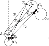
Figure III.1: Common Tangents $\{A_{p}(t),C_{e}(t)\}$

In order to design feedback laws we make use of the common tangents from the pursuer-circles to the evader-circles. Note that the pursuer-circles (evader-circles) at time $t$ depend only on the position and orientation of the pursuer (evader) at time instant $t$. Let $OC(t):=\{A_{p}(t),C_{p}(t),A_{e}(t),C_{e}(t)\}$ denote the set of pursuer-circles and evader-circles at time $t$. A $PE$-pair is a pair of circles with one circle belonging to the pursuer-circles and the other circle belonging to the evader-circles. Thus, in total we have four $PE$-pairs. The set of $PE$-pairs at time $t$ is denoted by $PE(t)$.

$$PE(t) := \{\{C_{p}(t),C_{e}(t)\},\,\{C_{p}(t),A_{e}(t)\},$$

$$\,\{A_{p}(t),C_{e}(t)\},\,\{A_{p}(t),A_{e}(t)\}\}$$

Between the two circles belonging to a $PE$-pair, whose centers are at a minimum distance of $r_{p}+r_{e}$ away from each other, there will be four tangents. These tangents have been shown in between the $PE$-pair $\{A_{p}(t),C_{e}(t)\}$ in Figure III.1. We assign direction to the tangents from the pursuer to the evader and we call them directed common tangents.

Definition 10.

Valid common tangent for a $PE-\text{pair}$ is a directed common tangent whose orientation matches with the direction of both the pursuer circle and the evader circle in the $PE-\text{pair}$.

In Figure III.1 only the tangent $T_{3}$ (shown by dashed line) is a valid tangent for pair $\{A_{p}(t),C_{e}(t)\}$.

Definition 11.

If a pursuer’s (evader’s) trajectory up to some time $t_{f}>0$ is such that it traverses one of the pursuer-circles (evader-circles) in time interval $[0,t^{\prime}]$ with $t^{\prime}\leq\min(t_{f},2\pi r_{p}/v_{p_{m}})$, and then traverses one of the tangents to that pursuer-circle (evader-circle) in time interval $[t^{\prime},t_{f}]$, then such a trajectory is of the type $CS$ (circle and straight line) up to time $t_{f}$.

Remark 12.

The condition $t^{\prime}\leq 2\pi r_{p}/v_{p_{m}}$ ensures that no part along the circumference of the circle is traversed more than once. If a trajectory of type $CS$ follows anticlockwise (left) circle and after that follows a straight line path then we say the trajectory belongs to the type $LS$. Similarly, if it follows clockwise (right) circle and after that follows a straight line path then we say the trajectory is of the type $RS$.

Definition 13.

If a pursuer’s (evader’s) trajectory up to time $t_{f}$ is such that it traverses one of the pursuer-circles (evader-circles) say $A_{p}(0)$ ($A_{e}(0)$) in time interval $[0,t^{\prime}]$ with $t^{\prime}\leq\text{min}(t_{f},2\pi r_{p}/v_{p_{m}})$, and then traverses the other pursuer-circle (evader-circle) i.e. $C_{p}(0)$ ($C_{e}(0)$) in the time interval $[t^{\prime},t_{f}]$, then such a trajectory is of the type $CC$ (circle-circle).

III-B Reachable sets of Dubins vehicle

Next, we describe the reachable sets of Dubins vehicle. Reachable set is used to characterize the solution for the game of two cars. The reachable set for the Dubins vehicle has been studied in [10, 11]. It is known that, the points inside the pursuer (evader) circles can be reached in minimum time by $CC$ (circle-circle) types of curves. The points external to the pursuer (evader) circles can be reached in minimum time by $CS$ type of curves. The external boundary of $R_{p}({\bf p_{0}},\bar{t})$ ($R_{e}({\bf p_{0}},\bar{t})$) is denoted by $\partial R_{p}({\bf p_{0}},\bar{t})$ ($\partial R_{e}({\bf e_{0}},\bar{t})$).

It is known [11] that, if $\bar{t}\geq 2\pi r_{p}/v_{p_{m}}$ ($\bar{t}\geq 2\pi r_{e}/v_{e_{m}}$) the points on $\partial R_{p}({\bf p_{0}},\bar{t})$ ($\partial R_{e}({\bf e_{0}},\bar{t})$) at time $\bar{t}$ can be reached only by the trajectories of the type $CS$. Thus $\partial R_{p}({\bf p_{0}},\bar{t})$ ($\partial R_{e}({\bf e_{0}},\bar{t})$) at $\bar{t}\geq 2\pi r_{p}/v_{p_{m}}$ ($\bar{t}\geq 2\pi r_{e}/v_{e_{m}}$) is comprised of two portions. The first portion is characterized by trajectories which begin on anti-clockwise circle and then follow a straight line. The second portion is characterized by trajectories which begin on the clockwise circle and then follow a straight line.

Consider the pursuer with initial state vector ${\bf p}(0)=\left[x_{0}\ y_{0}\ \theta_{0}\right]^{\top}$. The trajectories ${\bf p}\in\mathcal{C}(\mathbb{R}^{+},\mathbb{R}^{3})$ corresponding to the input

$$w_{p}(t) = +w_{p_{m}}\quad t\in[0,t_{1}]$$

$$w_{p}(t) = 0\quad t\in(t_{1},\bar{t}]$$

$$v_{p}(t) = v_{p_{m}}\quad t\in[0,\bar{t}]$$

for some $0\leq t_{1}\leq 2\pi r_{p}/v_{p_{m}}$, will initially follow the anti-clockwise circle and then travel on a tangent to the anti-clockwise circle. The pursuer moves up to time $\bar{t}>2\pi r_{p}/v_{p_{m}}$ with speed $v_{p_{m}}$ throughout. Since $2\pi r_{p}/v_{p_{m}}$ is the time required to travel a complete circle, it will cover a distance greater than circumference of the circle. (Note that the switching time $t_{1}$ is less than $2\pi r_{p}/v_{p_{m}}$ so that the no length of the circle is repeated). The trajectory is parameterized by the switching time $t_{1}$ and can be obtained by integrating (II.1) as

$$x_{fl}(\bar{t}) = x_{0}+(\sin(\tilde{\theta})-\sin(\theta_{0}))/w_{p_{m}}+v_{p_{m}}\cos(\tilde{\theta})\tilde{t}$$ (III.1)

$$y_{fl}(\bar{t}) = y_{0}-(\cos(\tilde{\theta})-\cos(\theta_{0}))/w_{p_{m}}+v_{p_{m}}\sin(\tilde{\theta})\tilde{t}$$

where $\tilde{\theta}=\theta_{0}+v_{p_{m}}w_{p_{m}}t_{1}$ and $\tilde{t}=\bar{t}-t_{1}$. Using these, the left reachable set of pursuer is defined as

$$R_{p}^{l}({\bf p_{0}},\bar{t}) = \{{\bf z}=[x\ y]^{\top}\in\mathbb{R}^{2}|x=x_{fl}(t)\ \text{and}\$$

$$\ y=y_{fl}(t)\ \forall\ t_{1}\leq\bar{t},t\leq\bar{t}\ \text{s.t.}t_{1}<t\}$$

The left reachable set for the evader $R_{e}^{l}({\bf e_{0}},\bar{t})$ is defined analogously. The left reachable set is shown in Figure III.4. The boundary of left reachable set of pursuer (evader) is denoted by $\partial R_{p}^{l}({\bf p_{0}},\bar{t})$ ($\partial R_{e}^{l}({\bf e_{0}},\bar{t})$).

For $\bar{t}\geq 2\pi r_{p}/v_{p_{m}}$ the right reachable sets for the pursuer $R_{p}^{r}({\bf p_{0}},\bar{t})$ and evader $R_{e}^{r}({\bf e_{0}},\bar{t})$ are defined similarly by the trajectories which first travel on the clockwise circle and then on the tangent to the clockwise circle. The right reachable set is shown in Figure III.4. The boundary of right reachable set of pursuer (evader) is denoted by $\partial R_{p}^{r}({\bf p_{0}},\bar{t})$ ($\partial R_{e}^{r}({\bf e_{0}},\bar{t})$).

The left reachable set and right reachable set of the pursuer (evader) are the subsets of the reachable set $R_{p}({\bf p_{0}},\bar{t})$ ($R_{e}({\bf e_{0}},\bar{t})$). The union of $R_{p}^{l}({\bf p_{0}},\bar{t})$ and $R_{p}^{r}({\bf p_{0}},\bar{t})$ is shown in Figure III.4.

The boundary of left reachable set is divided in two parts for $\bar{t}\geq 2\pi r_{p}/v_{p_{m}}$ in next definition.

Definition 14.

For $\bar{t}\geq 2\pi r_{p}/v_{p_{m}}$, the portion $ADE$ as shown in Figure III.4 will be called the left external boundary whereas the portion $EFB$ will be called the left internal boundary. Similarly, for the right reachable set the portion $ADE$ as shown in Figure III.4 will be called the right external boundary whereas the portion $EFB$ will be called the right internal boundary for $\bar{t}\geq 2\pi r_{p}/v_{p_{m}}$.

Remark 15.

The external boundary of the reachable set $\partial R_{p}({\bf p_{0}},\bar{t})$ ($\partial R_{e}({\bf e_{0}},\bar{t})$) is the union of left external boundary and the right external boundary for $\bar{t}\geq 2\pi r_{p}/v_{p_{m}}$. Note that the shape of the reachable sets is as shown in Figures III.4, III.4, III.4 only if $\bar{t}\geq 2\pi r_{e}/v_{e_{m}}\geq 2\pi r_{p}/v_{p_{m}}$.

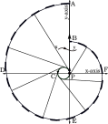
Figure III.2: Left reachable set ($R_{p}^{l}({\bf p_{0}},\bar{t})$)

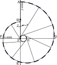
Figure III.3: Right reachable set ($R_{p}^{r}({\bf p_{0}},\bar{t})$)

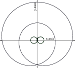
Figure III.4: $R_{p}^{r}({\bf p_{0}},\bar{t})\cup R_{p}^{l}({\bf p_{0}},\bar{t})$

IV Counter examples using reachable sets

The reachable set characterizes the points which the Dubins vehicle can reach in a given time. It would seem that the evader can always escape capture if the evader’s reachable set is not contained completely inside the pursuer’s reachable set. However, this is only possible if there exists an evader trajectory which can enter the region not contained in pursuer’s reachable set, without passing through the pursuer’s reachable set. For if the trajectory passes through the pursuer’s reachable set it will be intercepted by some pursuer’s trajectory. This notion is formalized in the next definition by introducing the safe region of the evader with respect to subsets of pursuer’s reachable set.

Definition 16.

The safe region of the evader, at time $\bar{t}$, with respect to a subset of pursuer’s reachable set $R_{p}^{s}({\bf p_{0}},\bar{t})\subset R_{p}({\bf p_{0}},\bar{t})$ is defined as

$$R_{e}^{-}({\bf e_{0}},R_{p}^{s},\bar{t}) = \{{\bf z}\in\mathbb{R}^{2}:{\bf z}\in R_{e}({\bf e_{0}},\bar{t})\backslash R_{p}^{s}({\bf p_{0}},\bar{t})\$$

$$\text{and }\exists\ \text{an evader}\text{ trajectory }$$

$$\text{with }{\bf e}_{|\mathbb{R}^{2}}(t_{1})={\bf z}\text{ for some }t_{1}\leq\bar{t},$$

$$\text{and }{\bf e}{}_{|\mathbb{R}^{2}}(t)\notin R_{p}^{s}({\bf p_{0}},t)\ \text{$\forall$}\ t\leq\bar{t}\}$$

Lemma 17.

Let $T_{l}$ be the minimum time such that $R_{e}^{-}({\bf e_{0}},R_{p}^{l},T_{l})=\emptyset$. If $d_{pe}^{0}\geq 2r_{p}+2\pi r_{p}(v_{e_{m}}/v_{p_{m}})$ then $T_{l}<\infty$.

Proof:

See Appendix. ∎

Lemma 18.

Let $T_{r}$ be the minimum time such that $R_{e}^{-}({\bf e_{0}},R_{p}^{r},T_{r})=\emptyset$. If $d_{pe}^{0}\geq 2r_{p}+2\pi r_{p}(v_{e_{m}}/v_{p_{m}})$ then $T_{r}<\infty$.

Lemma 19.

Let $T_{o}$ be the minimum time such that $R_{e}^{-}({\bf e_{0}},R_{p},T_{o})=\emptyset$. If $d_{pe}^{0}\geq 2r_{p}+2\pi r_{p}(v_{e_{m}}/v_{p_{m}})$ then $T_{o}<\infty$.

Proof:

Follows from Lemma 17 and Lemma 18. ∎

Remark 20.

It would seem that the condition $R_{e}^{-}({\bf e_{0}},R_{p},\bar{t})=\emptyset$, would be necessary and sufficient for capture. Let $T_{o}=\inf\{t\in\mathbb{R}:R_{e}^{-}({\bf e_{0}},R_{p},t)=\emptyset\}$. It is shown in [18], for pursuer and evader which can turn instantaneously, that such a condition is indeed necessary and sufficient for capture if we consider open-loop strategies and capture occurs at $T_{o}$. However, we demonstrate through the following counter-examples that the claim does not hold if we consider feedback strategies for the pursuer and evader.

Example 21.

Refer to Figure IV.3 where the evader is exactly behind the pursuer and oriented away from the pursuer. The pursuer’s initial position is ${\bf p_{0}}=[0,0,\pi/2]$ while that of the evader is ${\bf e_{0}}=[-11,0,-\pi/2]$. Assume $v_{p_{m}}=2$, $w_{p_{m}}=0.2$, $v_{e_{m}}=1.15$ and $w_{e_{m}}=0.18$. At time $T_{o}=31.34$, the evader’s reachable set (dotted curve) is contained in pursuer’s reachable set (solid line). If $R_{e}^{-}({\bf e_{0}},R_{p},T_{o})=\emptyset$ was the criterion for capture, then the evader would have traveled straight and the pursuer would have intercepted it along the $CS$ path exactly at the point marked by star in Figure IV.3. However, the optimal feedback strategies obtained by numerical simulation (using the algorithms in [24]) and the reachable set for such a strategy are as shown in Figure IV.3. Such a situation happens at time $T=35.9$. Hence, $R_{e}^{-}({\bf e_{0}},R_{p},T_{o})=\emptyset$ is not a sufficient criterion for capture.

Example 22.

An alternate hypothesis might be that capture occurs when either the left reachable set or the right reachable set completely contains the evader’s reachable region as shown in Figure IV.3. But consider the case when evader is in front of the pursuer as shown in Figure IV.3. Again the game is solved numerically using algorithms in [24]. At the point of capture, marked by the star, neither the left nor the right reachable set of the pursuer contain the evader’s reachable set.

Examples 21 and 22 indicate that reachable sets themselves do not characterize capture and a novel geometric interpretation is required to understand the nature of optimal trajectories. This is achieved next by introducing the notion of continuous subsets of reachable sets.

Figure IV.1: Invalid containment of evader’s reachable set

Figure IV.2: Valid containment of evader’s reachable set

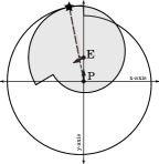
Figure IV.3: Left reachable set does not contain evader’s reachable set. Yet capture occurs at this time.

V Continuous subsets of reachable set

Recall that $T_{o}=\inf\{t\in\mathbb{R}:R_{e}^{-}({\bf e_{0}},R_{p},t)=\emptyset\}$ and consider a point ${\bf z}\in\partial R_{e}({\bf e}_{0},T_{o})\cap\partial R_{p}({\bf p}_{0},T_{o})$. In Example 21 it was shown that the capture did not occur at point ${\bf z}$. We try to explain this phenomena using small deviations around the evader input signal. This will result in a small deviation in the final point ${\bf e}_{|\mathbb{R}^{2}}(T_{o})={\bf z}$.

Observation: If capture is to occur at ${\bf z}={\bf e}_{|\mathbb{R}^{2}}(T_{o})$, using feedback pursuer strategies, every feasible variation in ${\bf e}$ should be traceable by the pursuer using small variations of its own input signal.

We make the notion of admissible variations more concrete in this section by defining the continuous subsets of the reachable set for the Dubins vehicle.

Definition of Continuous Subsets of Reachable Sets

Let $R_{p}({\bf p_{0}},\bar{t})$ be the reachable set of the pursuer at time $\bar{t}$ starting from initial position ${\bf p}_{0}\in\mathbb{R}^{3}$.

1. Let ${\bf x,y}\in R_{p}({\bf p_{0}},\bar{t})$ and let $\overline{{\bf xy}}$ be any curve from ${\bf x}$ to ${\bf y}$ such that all points on $\overline{{\bf xy}}$ belong to $R_{p}({\bf p_{0}},\bar{t})$ as shown in Figure VII.3.

2. Let $\mathfrak{T}_{\overline{{\bf x}{\bf y}}}({\bf r},{\bf p_{0}},\bar{t})$ be the set of all the trajectories from ${\bf p_{0}}$ to the point ${\bf r}$ on $\overline{{\bf x}{\bf y}}$, which reach the point ${\bf r}\in R_{p}({\bf p_{0}},\bar{t})$ at time $t\leq\bar{t}$ starting from ${\bf p_{0}}$.

   $$\mathfrak{T}_{\overline{{\bf x}{\bf y}}}({\bf r},{\bf p_{0}},\bar{t}) = \{{\bf p}\in\mathcal{C}^{0}(\mathbb{R}^{+},\mathbb{R}^{3}):\exists\,\,{\bf u_{p}}\in\mathcal{U}_{p}\,$$

   $$\text{ with }{\bf p}_{|\mathbb{R}^{2}}(t)={\bf r}$$

   $$\,\,\,\text{ and }{\bf p}(0)={\bf p_{0}}\ \text{for }\text{some }t\leq\bar{t}\}$$

3. Let $\mathfrak{L}(\overline{{\bf x}{\bf y}},{\bf p_{0}},\bar{t})$ be the collection of all possible trajectories from ${\bf p_{0}}$ which reach line $\overline{{\bf x}{\bf y}}$ at time $t\leq\bar{t}$ .

   $$\mathfrak{L}(\overline{{\bf x}{\bf y}},{\bf p_{0}},\bar{t}) = \Big{\{}{\bf p}\in\mathcal{C}^{0}(\mathbb{R}^{+},\mathbb{R}^{3}):\exists\ {\bf r}\in\overline{{\bf x}{\bf y}}\ \text{s.t.}$$

   $$\ {\bf p}\in\mathfrak{T}_{\overline{{\bf x}{\bf y}}}({\bf r},{\bf p_{0}})\Big{\}}$$

4. Now we look at functions $\mathfrak{f}:\overline{{\bf x}{\bf y}}\rightarrow\mathfrak{L}(\overline{{\bf x}{\bf y}},{\bf p_{0}},\bar{t})$ such that $\mathfrak{f}({\bf r})\in\mathfrak{T}_{\overline{{\bf x}{\bf y}}}({\bf r},{\bf p_{0}},\bar{t})$ $\forall\ {\bf r}\in\overline{{\bf xy}}$. We construct a set $\mathfrak{C}(\overline{{\bf x}{\bf y}},{\bf p_{0}},\bar{t})$ such that

   $$\mathfrak{C}(\overline{{\bf x}{\bf y}},{\bf p_{0}},\bar{t}) = \{\mathfrak{f}|\mathfrak{f}:\overline{{\bf x}{\bf y}}\rightarrow\mathfrak{L}(\overline{{\bf x}{\bf y}},{\bf p_{0}},\bar{t})\ \text{and }$$

   $$\mathfrak{f}({\bf r})\in\mathfrak{T}_{\overline{{\bf x}{\bf y}}}({\bf r},{\bf p_{0}},\bar{t})\forall\ {\bf r}\in\overline{{\bf xy}}\}$$

   The set $\mathfrak{C}(\overline{{\bf x}{\bf y}},{\bf p_{0}},\bar{t})$ is the set of all the functions which map some point ${\bf r}\in\overline{{\bf x}{\bf y}}$ to a trajectory ${\bf p}\in\mathfrak{L}(\overline{{\bf x}{\bf y}},{\bf p_{0}},\bar{t})$ and the trajectory ${\bf p}$ is such that ${\bf p}_{|\mathbb{R}^{2}}(\bar{t})={\bf r}$.

5. Let the metric be defined on set $\overline{{\bf x}{\bf y}}$ by the standard two norm. The metric on the set $\mathfrak{L}(\overline{{\bf x}{\bf y}},{\bf p_{0}},\bar{t})$ is defined by the $\mathcal{L}_{\infty}$ norm.

Definition 23.

We say that the curve $\overline{{\bf x}{\bf y}}$ is a continuum set if there exists a continuous one-one map $\mathfrak{f}^{c}\in\mathfrak{C}(\overline{{\bf x}{\bf y}},{\bf p_{0}},\bar{t})$.

Definition 24.

The range of $\mathfrak{f}^{c}$ will be called the continuum of trajectories.

Remark 25.

Since, $\mathfrak{f}^{c}$ is a continuous function, the trajectories in the continuum of trajectories of $\mathfrak{f}^{c}$ are such that for any two points ${\bf w,z}\in\overline{{\bf x}{\bf y}}$ we have $||\mathfrak{f}^{c}({\bf w})-\mathfrak{f}^{c}({\bf z})||_{\mathcal{L}_{\infty}}\rightarrow 0$ as $||{\bf w}-{\bf z}||_{2}\rightarrow 0$.

Definition 26.

A continuous subset of the reachable set at time $\bar{t}$, $R_{p}^{c}({\bf p_{0}},\bar{t})\subseteq R_{p}({\bf p_{0}},\bar{t})$ is a connected set of all the points s.t.

1. For all ${\bf x,y}\in R_{p}^{c}({\bf p_{0}},\bar{t})$ and every curve $\overline{{\bf x}{\bf y}}\in R_{p}^{c}({\bf p_{0}},\bar{t})$, the set $\overline{{\bf x}{\bf y}}$ is a continuum set.

2. For every point ${\bf r}\in R_{p}^{c}({\bf p_{0}},\bar{t})$ there exists a trajectory ${\bf p}\in\mathcal{C}^{0}(\mathbb{R}^{+},\mathbb{R}^{3})$ such that ${\bf p}(0)={\bf p_{0}},{\bf p}(\tilde{t})={\bf r}$ for some $0\leq\tilde{t}\leq\bar{t}$ and ${\bf p}(t)\in R_{p}^{c}({\bf p_{0}},\bar{t})$ for all $t\leq\bar{t}$.

From here on we will denote a continuous subset of pursuer’s reachable set by $CSP$. A continuous subset of the reachable set of the evader is defined analogously and will be denoted by $CSE$. From the definition it is clear that the continuous subsets of reachable set are not unique. The collection of all the $CSP$ ($CSE$) at time $\bar{t}$ from initial position ${\bf p_{0}}$ (${\bf e_{0}}$) is denoted by $\mathfrak{R}_{p}({\bf p_{0}},\bar{t})$ ($\mathfrak{R}_{e}({\bf e_{0}},\bar{t})$).

$$\mathfrak{R}_{e}({\bf e_{0}},\bar{t}) = \{R_{e}^{c}({\bf e_{0}},\bar{t}):R_{e}^{c}({\bf e_{0}},\bar{t})\subseteq R_{e}({\bf e_{0}},\bar{t})\}$$

$$\mathfrak{R}_{p}({\bf p_{0}},\bar{t}) = \{R_{p}^{c}({\bf p_{0}},\bar{t}):R_{p}^{c}({\bf p_{0}},\bar{t})\subseteq R_{p}({\bf p_{0}},\bar{t})\}$$

The continuous safe region of a evader’s continuous subset $R_{e}^{c}({\bf e_{0}},\bar{t})\in\mathfrak{R}_{e}({\bf e_{0}},\bar{t})$ with respect to a continuous subset of the pursuer $R_{p}^{c}({\bf p_{0}},\bar{t})\in\mathfrak{R}_{p}({\bf p_{0}},\bar{t})$ is defined next.

Definition 27.

The continuous safe region $R_{e}^{c-}({\bf e_{0}},R_{p}^{c},\bar{t})$ of a $CSE$ $R_{e}^{c}({\bf e_{0}}$$,\bar{t})$, at time $\bar{t}$, with respect to a $CSP$ $R_{p}^{c}({\bf p_{0}},\bar{t})$ is defined as

$$R_{e}^{c-}({\bf e_{0}},R_{p}^{c},\bar{t}) = \{{\bf z}\in\mathbb{R}^{2}:{\bf z}\in R_{e}^{c}({\bf e_{0}},\bar{t})\backslash R_{p}^{c}({\bf p_{0}},\bar{t})\$$

$$\text{and }\exists\ \text{an evader}\text{ trajectory with}$$

$${\bf e}_{|\mathbb{R}^{2}}(t_{1})={\bf z}\text{ for some}\ t_{1}\leq\bar{t}\text{ and }$$

$${\bf e}_{|\mathbb{R}^{2}}(t)\notin R_{p}^{c}({\bf p_{0}},t)\ \text{at each}\ t\leq t_{1}\}$$

When the safe region is an empty set we say that the $CSP$ $R_{p}^{c}({\bf p_{0}},\bar{t})$ contains $CSE$ $R_{e}^{c}({\bf e_{0}},\bar{t})$ continuously.

Definition 28.

Continuous containment: If the continuous safe region of a $CSE$ $R_{e}^{c}({\bf e_{0}},\bar{t})$, at time $\bar{t}$, with respect to $CSP$ $R_{p}^{c}({\bf p_{0}},\bar{t})$ be such that $R_{e}^{c-}({\bf e_{0}},R_{p}^{c},\bar{t})=\emptyset$, then we say that $R_{p}^{c}({\bf p_{0}},\bar{t})$ contains $R_{e}^{c}({\bf e_{0}},\bar{t})$ continuously.

It turns out that optimal capture occurs when every continuous subset of the evader is contained inside some continuous subset of the pursuer. The time $T$ at which such a situation occurs is defined next. Let

$$T := \inf\{t\in\mathbb{R}:\forall\ R_{e}^{c}({\bf e_{0}},t)\in\mathfrak{R}_{e}({\bf e_{0}},t)\$$

$$\text{$\exists$}\ R_{p}^{c}({\bf p_{0}},t)\in\mathfrak{R}_{p}({\bf p_{0}},t)\ \text{s.t. }R_{e}^{c-}({\bf e_{0}},R_{p}^{c},t)=\emptyset\}$$

VI Main Results

In this section we state the main contributions of the paper. These have been proved in subsequent sections.

VI-A Capture characterization using continuous subsets

The next theorem states that the minimum time at which continuous containment occurs ($T$ as defined by (V)) is the same as the $\min-\max$ time ($T^{*}$ as per Definition 2) $T=T^{*}$. This implies that for all time $t<T=T^{*}$ there exists an evader feedback policy such that irrespective of any feedback policy of the pursuer, the evader is able to avoid capture. Also, there exists a feedback pursuer policy such that irrespective of any feedback policy of the evader the pursuer is able to capture it at some time $t<T=T^{*}$.

Theorem 29.

Let $T$ and $T^{*}$ be as per (V) and Definition 2. $T$ is the $\min-\max$ time to capture i.e. $T=T^{*}$.

Proof:

See Section VIII. ∎

Theorem 29 demonstrates that continuous containment is a complete characterization of optimal capture. However, to completely understand the nature of the optimal trajectories we investigate the specific continuous subsets of the pursuer and evader reachable sets that actually achieve the inf $T$ in (V). Through a careful study of these special $CSE/CSP^{\prime}s$ we are able to prove the following theorem that describes the optimal trajectories.

Theorem 30.

If the initial distance $d_{pe}^{0}\geq 2r_{e}+2\pi r_{e}(v_{p_{m}}/v_{e_{m}})$, then the saddle-point strategies of the evader and the pursuer are of the type $CS$ that is a circle and straight line.

Proof:

See Section IX. ∎

The trajectories of both the pursuer and the evader are of the type $CS$ and since it is guaranteed that capture will occur, the straight lines are coincident to the capture point. This observation allows us to prove the next geometric result.

Theorem 31.

If $d_{pe}^{0}\geq 2r_{e}+2\pi r_{e}(v_{p_{m}}/v_{e_{m}})$ then the saddle-point strategies of the pursuer and the evader result in pursuer and evader trajectories being coincident to circles in an $PE$-pairs and one of the common tangents of that pair.

Proof:

See Section X. ∎

Clearly Theorem 31 effectively solves the subsidiary Problem 6 listed in Section II. The simple geometry of optimal curves defined by Theorem 31 lets us propose an algorithm to immediately compute the feedback control for both the pursuer and the evader at each instant. This solution to Problem 4 is described next.

VI-B Feedback law using geometry

In this section we design algorithms to select an appropriate tangent which describes the feedback saddle-point strategies. As discussed in Section III-A each $PE$-pair has four common tangents. Since there are four such $PE$-pairs we will have 16 directed tangents in total. First we show that at any time $t$, only one directed tangent corresponding to each $PE$-pair in the set $PE(t)$ is a valid tangent along which the saddle-point trajectories may occur.

Lemma 32.

At each time $t$, corresponding to each pair of $PE$-circles in the set $PE(t)$ there is only one valid common tangent with which saddle point strategies can coincide.

Proof:

We prove this on a case by case basis. Consider a circle pair $\{A_{p}(t),C_{e}(t)\}\in PE(t)$ as shown in Figure III.1. A directed straight line $\overrightarrow{O_{p}O_{e}}$ is drawn from the center of circle $A_{p}$ to the center of circle $C_{e}$. Clearly, the tangents which end on the evader to the right of $\overrightarrow{O_{p}O_{e}}$ are not feasible as the direction of the tangents do not match with the orientation of the evader. Similarly, the tangents which end on $C_{e}(t)$ to the left of the line $\overrightarrow{O_{p}O_{e}}$ are also not feasible. Hence, we can eliminate tangents $T_{1}$, $T_{2}$ and $T_{4}$. Thus, only the tangent $T_{3}$ (dashed line) is a feasible one. Similarly, the claim can be proven for other pairs in the set $PE(t)$. ∎

Algorithm 1 is designed to compute the valid tangent for each $PE$-pair. The common tangents of all the $PE$-pairs have been shown in Figures III.1, VI.3, VI.3, and VI.3. In each case the valid tangent has been shown by a dashed line.

1. For the tangent under consideration let $T_{p}$ be its intersection point with the pursuer circle under consideration and $T_{e}$ be the intersection point with the evader circle under consideration.

2. The following observations can be seen from Figures III.1, VI.3, VI.3, and VI.3 for valid tangent.

   1. For $A_{p}(t)$ and $A_{e}(t)$ the angle between the valid tangent and $\overrightarrow{O_{p}T_{p}}$ and $\overrightarrow{O_{e}T_{e}}$ translated to $T_{p}$ and $T_{e}$ respectively is $\pi/2$ in anti-clockwise direction.

   2. For $C_{p}(t))$ and $C_{e}(t)$ the angle between the valid tangent and $\overrightarrow{O_{p}T_{p}}$ and $\overrightarrow{O_{e}T_{e}}$ translated to $T_{p}$ and $T_{e}$ respectively is $-\pi/2$ in anti-clockwise direction.

3. For a given directed tangent $\overrightarrow{T}$ in a $PE$-pair if the angles with $\overrightarrow{O_{p}T_{p}}$ and $\overrightarrow{O_{e}T_{e}}$ satisfy the conditions above then it is a valid tangent.

Algorithm 1 Valid Tangent

It was shown, using geometry, in Lemma 32 that each $PE$-pair has only one valid tangent. Thus there are four valid tangents (one corresponding to each $PE$-pair) with which the saddle-point strategies of the pursuit-evasion game may coincide. Next we formulate a matrix game at each instant of time to design feedback saddle-point strategies for the pursuit-evasion game.

Recall that the clockwise circle $C_{p}(t)$ is traversed for $w_{p}(t)=-w_{p_{m}}$ and anticlockwise circle $A_{p}(t)$ for $w_{p}(t)=+w_{p_{m}}$. Similarly, for the evader the clockwise circle $C_{e}(t)$ is traversed for $w_{e}(t)=-w_{e_{m}}$ and anticlockwise circle $A_{e}(t)$ for $w_{e}(t)=+w_{e_{m}}$. Selecting $w_{p}(t)=+w_{p_{m}}$ and $w_{e}(t)=-w_{e_{m}}$ is equivalent to selecting the valid tangent of the pair $\{A_{p}(t),C_{e}(t)\}$ along which saddle-point strategies for the pursuit-evasion game will occur. The computation of time to capture at time $t$, $T_{ac}(t)$, for the valid tangent of the pair $\{A_{p}(t),C_{e}(t)\}$, shown in Figure III.1, is given in Algorithm 2.

Input: Valid tangent for the pair $\{A_{p}(t),C_{e}(t)\}$

 

Let $ET_{e}$ be the arc subtended between $O_{e}E$ and $O_{e}T_{e}$ in clockwise direction and let $PT_{p}$ be the arc subtended by $O_{p}P$ and $O_{p}T_{p}$ in anticlockwise direction as shown in Figure III.1. Compute the length of the arcs $PT_{p}=l_{ap}$ and $ET_{E}=l_{a_{e}}$ and define $t_{p}:=l_{ap}/v_{p_{m}}$ and $t_{e}:=l_{ae}/v_{e_{m}}$. Also, let the distance between $T_{p}T_{e}$ be denoted by $d$.

1. If $t_{p}>t_{e}$ the evader will come out of the circle and onto the tangent earlier than the evader.

   1. $\tilde{t}:=t_{p}-t_{e}$. Thus the evader will travel a distance $d_{e}:=v_{e_{m}}\tilde{t}$ on the straight line before the pursuer comes onto the tangent.

   2. Thus at the time $t_{p}$ the distance between the pursuer and evader will be $\tilde{d}:=d+d_{e}$. Now the time to capture from this point will be $\bar{t}:=\tilde{d}/(v_{p_{m}}-v_{e_{m}})$.

   3. Thus the time to capture will be $T_{ac}(t)=t_{p}+\bar{t}$.

2. If $t_{p}\leq t_{e}$ the pursuer will come on straight line earlier.

   1. $\tilde{t}:=t_{e}-t_{p}$. Thus the pursuer will travel a distance $d_{p}:=v_{p_{m}}\tilde{t}$ on the straight line before the pursuer comes on the straight line.

   2. Thus at the time $t_{e}$ the distance between the pursuer and evader will be $\tilde{d}:=d-d_{p}$. Now the time to capture from this point will be $\bar{t}:=\tilde{d}/(v_{p_{m}}-v_{e_{m}})$.

   3. Thus the time to capture will be $T_{ac}(t)=t_{e}+\bar{t}$.

 

Output: Time to capture along a valid tangent for $\{A_{p}(t),C_{e}(t)\}$ pair $=$ $T_{ac}(t)$

Algorithm 2 Algorithm to compute time to capture along a valid tangent for $\{A_{p}(t),C_{e}(t)\}$ pair

Figure VI.1: $\{A_{p}(t),A_{e}(t)\}$

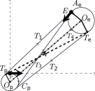
Figure VI.2: $\{C_{p}(t),A_{e}(t)\}$

Figure VI.3: $\{C_{p}(t),C_{e}(t)\}$

We calculate the times corresponding to each circle pairs and hence each input pairs. At an given time instant, say $t$, let $A_{p}(t)$, $C_{p}(t)$, and $A_{e}(t)$, $C_{e}(t)$ be the pursuer and evader circles respectively. Let $T_{aa}(t)$, $T_{ac}(t)$, $T_{ca}(t)$ and $T_{cc}(t)$ be the times corresponding to valid tangents of circle-pairs $\{A_{p}(t),A_{e}(t)\}$, $\{A_{p}(t),C_{e}(t)\}$, $\{C_{p}(t),C_{e}(t)\}$, and $\{C_{p}(t),C_{e}(t)\}$ respectively. For example, if the pursuit-evasion saddle-point occurs on the $PE$-pair $\{A_{p}(t),C_{e}(t)\}$ then at $t$ we must have $w_{p}(t)=w_{p_{m}}$ and $w_{e}(t)=-w_{e_{m}}$ initially. Similarly we have,

1. $\{A_{p}(t),A_{e}(t)\}\Rightarrow w_{p}(t)=+w_{p_{m}},\,w_{e}(t)=+w_{e_{m}}$

2. $\{A_{p}(t),C_{e}(t)\}$ $\Rightarrow$ $w_{p}(t)=+w_{p_{m}}$, $w_{e}(t)=-w_{e_{m}}$

3. $\{C_{p}(t),A_{e}(t)\}$ $\Rightarrow$ $w_{p}(t)=-w_{p_{m}}$, $w_{e}(t)=+w_{e_{m}}$

4. $\{C_{p}(t),C_{e}(t)\}$ $\Rightarrow$ $w_{p}(t)=-w_{p_{m}}$, $w_{e}(t)=-w_{e_{m}}$

until the time that the trajectory leaves the corresponding circle and starts on the straight line path along the common tangent. Thus corresponding to pursuer and evader inputs at time $t$, we obtain times of capture along each of the valid tangents. Using these times we formulate a matrix game as shown in Table I. The valid tangent on which the pursuit-evasion game occurs constitutes the saddle point strategies for the pursuit-evasion differential game. Thus, starting at time $t$ with the configuration ${\bf p}(t),\,{\bf e}(t)$, the saddle-point solution of the matrix game at each instant $t$ will give the common tangent, with which the open-loop representation of the feedback saddle-point strategies is coincident.

P\E	$w_{e}(t)=+w_{e_{m}}$	$w_{e}(t)=-w_{e_{m}}$
$w_{p}(t)=+w_{p_{m}}$	$T_{aa}(t)$	$T_{ac}(t)$
$w_{p}(t)=-w_{p_{m}}$	$T_{ca}(t)$	$T_{cc}(t)$

Table I: Matrix game at time instant $t$

Thus the policy of the evader would be $\max-\min$ solution of the matrix game while that of the evader would be $\min-\max$ solution of the matrix game at each instant $t$. From this discussion the next theorem follows.

Theorem 33.

If $d_{pe}^{0}\geq 2r_{e}+2\pi r_{e}(v_{p_{m}}/v_{e_{m}})$, the tangents selected by the saddle-point equilibrium in the matrix game described by Table I will be coincident with the open-loop representation of feedback saddle-point strategies at each time $t\geq 0$.

If the solution is computed at each instant of time $t$ and the input value corresponding to time instant $t$ i.e. $w_{p}(t)$ and $w_{e}(t)$ is applied then it constitutes a feedback law. Using Theorem 33, such a feedback law $\text{F}({\bf x}(t)):{\bf x}(t)\in\mathbb{R}^{6}\rightarrow[{\bf u_{p}^{\top}}(t)\,\,{\bf u_{e}^{\top}}(t)]^{\top}\in\mathbb{R}^{4}$ can be computed and this provides solution for Problem 4. For further details the interested reader can refer to Algorithm 3 in [25] for details.

VI-C Numerical Simulations

In [24], an algorithm is proposed to solve pursuit-evasion games numerically. This is achieved by first solving the $\min$ problem of the pursuer and then the $\max$ problem of the evader. These optimal problems are solved iteratively to obtain the $\min-\max$ solution of the differential game. We use their algorithm to numerically solve the game of two cars and the $\min$ and the $\max$ problems are solved using direct numerical optimal control methods [26] using IPOPT [27]. Clearly, such numerical techniques are not practical for computing feedback solution in real time due to time complexity and convergence issues of numerical optimization methods. However, we do these simulations in order to verify the correctness of the feedback law proposed in Theorem 33.

The parameters for the pursuer and evader used for simulations are $v_{p_{m}}=2$, $w_{p_{m}}=2$, $v_{e_{m}}=1$ and $w_{e_{m}}=1$. The simulations were performed using numerical techniques (NT) from [24] as well as the proposed feedback law (FL) for following initial states of the pursuer and the evader:

1. ${\bf{\bf p_{0}}}=[0,0,\pi/2],{\bf e_{0}}=[-3,-6,\pi/2]$ (ML: Figure VI.7, NT: Figure VI.11)

2. ${\bf p_{0}}=[0,0,\pi/2],{\bf e_{0}}=[6,3,\pi/2]$ (ML: Figure VI.7, NT: Figure VI.11)

3. ${\bf p_{0}}=[0,0,\pi/2],{\bf e_{0}}=[0,-6,\pi/2]$ (ML: Figure VI.7, NT: Figure VI.11)

4. ${\bf p_{0}}=[0,0,\pi/2],{\bf e_{0}}=[0,6,\pi/2+\pi/6]$ (ML: Figure VI.7, NT: Figure VI.11)

In all the figures the pursuer trajectory is shown by the dashed curve whereas the evader trajectory is shown by the dotted curve. The comparison of matrix law and the numerical simulation show that the trajectories are identical.

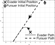
Figure VI.4: Feedback law-1

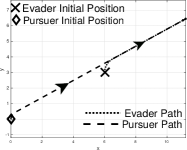
Figure VI.5: Feedback law-2

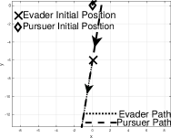
Figure VI.6: Feedback law-3

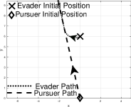
Figure VI.7: Feedback law-4

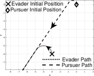
Figure VI.8: [24]Numerical -1

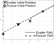
Figure VI.9: [24]Numerical -2

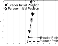
Figure VI.10: [24]Numerical -3

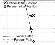
Figure VI.11: [24]Numerical -4

VII Proofs of continuity for specific subsets of the reachable set of Dubins vehicle

In this section we discuss the important continuous subsets of the reachable set of Dubins vehicle necessary to characterize the saddle-point trajectories for the game of two cars.

Definition 34.

Let $\overline{{\bf xy}}$ be a continuum set. If a continuum of trajectories for the curve $\overline{{\bf xy}}$ are of the type $LS$ then we say that $\overline{{\bf xy}}$ is a $LS$ continuum set. $RS,CS$ continuum sets are defined analogously.

Lemma 35.

Let $\bar{t}\geq 2\pi r_{p}/v_{p_{m}}$ and consider Figure III.4. Any curve $\overline{{\bf xy}}\in R_{p}^{l}({\bf p_{0}},\bar{t})$ such that $\overline{{\bf xy}}$ crosses the line $PA$, is not a $LS$ continuum set.

Proof:

Recall that the switching time $t_{1}$ for $LS$ type trajectory is less than $2\pi r_{p}/v_{p_{m}}$. The portion of the curve $\overline{{\bf xy}}$ on the left of $PA$ can be reached by $LS$ trajectories which have switching time $t_{1}\leq\pi r_{p}/v_{p_{m}}$ while the portion on right of $PA$ can be reached by curves with switching time $t_{1}\geq(3\pi/2)r_{p}/v_{p_{m}}$. Hence, there do not exist $LS$ trajectories which can make $\overline{{\bf xy}}$ a continuum set. ∎

Lemma 36.

Let $\bar{t}\geq 2\pi r_{p}/v_{p_{m}}$ and consider Figure VII.3. Any curve $\overline{{\bf xy}}\in R_{p}^{l}({\bf p_{0}},\bar{t})\backslash PA$ is a $LS$ continuum set.

Proof:

Recall that the switching time $t_{1}$ for a $LS$ trajectory is less than $2\pi r_{p}/v_{p_{m}}$. Consider a curve $\overline{{\bf xy}}$ in the reachable set of the kinematic point, between points ${\bf x},{\bf y}\in R_{p}^{l}({\bf p_{0}},\bar{t})$. Let ${\bf p_{x}}$ be a time optimal trajectory given by (III.1) and ${\bf x}={\bf p_{x}}_{|\mathbb{R}^{2}}(t)=[x_{f}(t)\ y_{f}(t)]^{\top}$ for some $t\leq\bar{t}$. Let ${\bf x^{\prime}}$ be a point in neighborhood of ${\bf x}$ such that ${\bf x^{\prime}}={\bf x}+\delta{\bf x}$, ${\bf x^{\prime}}\in R_{p}^{l}({\bf p_{0}},\bar{t})$ and ${\bf x^{\prime}}={\bf p^{\prime}_{x}}_{|\mathbb{R}^{2}}(t^{\prime})=[x_{f}(t^{\prime})\ y_{f}(t^{\prime})]^{\top}$ for some $t^{\prime}\leq\bar{t}$. Now define a function say ${\bf\bar{g}}:\mathbb{R}^{2}\rightarrow\mathbb{R}^{2}$ given by (III.1). The domain of the function is $t\times\theta\in\mathbb{R}^{2}$ where, $t\in[0,\bar{t}]$ and $\theta\in[0,2\pi]$ and the range is the set of points in the reachable set $R_{p}^{l}({\bf p_{0}},\bar{t})$. Now, the Jacobian of the function is,

$$J=\left[\begin{array}[]{cc}v_{p_{m}}\cos\tilde{\theta}&\ \ -v_{p_{m}}^{2}w_{p_{m}}(t-t_{1})\sin\tilde{\theta}\\ v_{p_{m}}\sin\tilde{\theta}&\ \ v_{p_{m}}^{2}w_{p_{m}}(t-t_{1})\cos\tilde{\theta}\end{array}\right]$$

Since (III.1) is defined such that $t>t_{1}>0$, $J$ is non-singular. Hence, by the inverse function theorem there exists an inverse map ${\bf\bar{g}}^{-1}:\mathbb{R}^{2}\rightarrow\mathbb{R}^{2}$ such that ${\bf\bar{g}}^{-1}$ is continuous. Thus, as $||\delta{\bf x}||_{2}\rightarrow 0$ we have $||[\delta t\ \delta\theta]^{\prime}||_{2}\rightarrow 0$ and thus $||{\bf p_{x}}_{|\mathbb{R}^{2}}-{\bf p^{\prime}}_{|\mathbb{R}^{2}}||_{\mathcal{L_{\infty}}}\rightarrow 0$. Thus, for any two nearby points the trajectories will also be nearby.

Define a function $\mathfrak{f}$ such that it matches each point ${\bf x}$ to the time-optimal trajectory given by (III.1) and ${\bf x}={\bf p_{x}}_{|\mathbb{R}^{2}}(t_{a})=[x_{fl}(t_{a})\ y_{fl}(t_{a})]$ for some $t_{a}\leq\bar{t}$. Thus the function $\mathfrak{f}$ would be a one-one function by definition. Also, the function is also continuous by the analysis presented above ($||\delta{\bf x}||_{2}\rightarrow 0\Rightarrow||{\bf p_{x}}_{|\mathbb{R}^{2}}-{\bf p^{\prime}}_{|\mathbb{R}^{2}}||_{\mathcal{L_{\infty}}}\rightarrow 0$). Thus $\overline{{\bf xy}}$ is a continuum set. ∎

The following lemma is analogous to Lemma 36.

Lemma 37.

Let $\bar{t}\geq 2\pi r_{p}/v_{p_{m}}$. Any curve $\overline{{\bf xy}}\in R_{p}^{r}({\bf p_{0}},\bar{t})\backslash PA$ is a $RS$ continuum set.

Next, we define a series of special continuous subsets of reachable sets, which will be useful to characterize the saddle point capture condition in Section IX-A and Section IX-B.

Definition 38.

Let $\bar{t}\geq 2\pi r_{p}/v_{p_{m}}$. Then, the central reachable set of the pursuer (see Figure VII.3) is defined as $R_{p}^{CR}({\bf p_{0}},\bar{t})=R_{p}({\bf p_{0}},\bar{t})\backslash\{\text{int}(C_{p}(0))\cup\text{int}(A_{p}(0))\cup\overline{PB}\}$, where $\text{int}(C_{p}(0))$ and $\text{int}(A_{p}(0))$ denote the interiors of pursuer circles at time $t=0$ and $\overline{PB}=\{PB\backslash\{P\}\}$.

The central reachable set of the evader $R_{e}^{CR}({\bf e_{0}},\bar{t})$ is defined analogously for $\bar{t}\geq 2\pi r_{e}/v_{e_{m}}$. The central reachable set is shown in Figure VII.3. The points on the line segment $\overline{PB}$ and the area inside the minimum turning radius circles do not form a part of central reachable set.

Lemma 39.

The central reachable set of pursuer/evader is a continuous subset for all time $t\geq 2\pi\frac{r_{p}}{v_{p_{m}}}$ ($t\geq 2\pi\frac{r_{e}}{v_{e_{m}}}$ ).

Proof:

Consider Figure VII.3. Let $D_{l}$ denote the set of points enclosed by the curve $DABPD$ and $D_{r}$ be the set of points enclosed by the curve $DCBPD$. Any curve contained completely in the set $D_{l}\backslash\left(\overline{PB}\cup\text{int}(A_{p}(0))\right)\subseteq R_{p}^{l}({\bf p_{0}},\bar{t})$ is a continuum set by Lemma 36. Also, any curve contained completely in the set $D_{r}\backslash\left(\overline{PB}\cup\text{int}(A_{p}(0))\right)$
$\subseteq R_{p}^{r}({\bf p_{0}},\bar{t})$ is a continuum set by Lemma 37. Thus we need to consider only those type of curves which cross line $DP$ such as the curve ${\bf x-z}-{\bf y}$ shown in Figure VII.3. The curve $\overline{{\bf xz}}$ in Figure VII.3 is a $LS$ continuum set. Let this continuum set of trajectories be denoted by ${\bf T^{l}}$. Similarly, any curve $\overline{{\bf zy}}$ in the subset $DCBPD\subseteq R_{p}^{r}({\bf p_{0}},\bar{t})$ as shown in Figure VII.3 is a continuous subset with $RS$ type of trajectories. Let this continuum of trajectories be denoted by ${\bf T^{r}}$. Now, the trajectory in ${\bf T^{l}}$ and ${\bf T^{r}}$ which reaches the point ${\bf z}$ is the same trajectory along the straight line $PD$. Thus, ${\bf T^{l}}\cup{\bf T^{r}}$ forms a continuum of trajectories for the curve ${\bf x-z}-{\bf y}$ and hence it is a continuum set. Thus any curve in the central reachable set is a continuum set with $CS$ type of trajectories. Further, the continuum of trajectories ${\bf T^{l}}\cup{\bf T^{r}}$ is completely contained in $R_{p}^{CR}({\bf p_{0}},\bar{t})$. Hence, the central reachable set it is a continuous subset. ∎

Figure VII.1: Continuum of trajectories

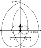
Figure VII.2: $R_{p}^{r}({\bf p_{0}},\bar{t})\cup R_{p}^{l}({\bf p_{0}},\bar{t})$ is not a $CSP$.

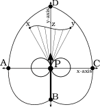
Figure VII.3: Central reachable set is a continuous subset

Definition 40.

Consider Figures III.4 and III.4 and let $\bar{t}\geq 2\pi r_{p}/v_{p_{m}}$. The truncated left reachable set is defined as $R_{p}^{l_{t}}({\bf p_{0}},\bar{t}):=R_{p}^{l}({\bf p_{0}},\bar{t})\backslash PA$. Similarly, the truncated right reachable set is defined as $R_{p}^{r_{t}}({\bf p_{0}},\bar{t})=R_{p}^{r}({\bf p_{0}},\bar{t})\backslash PA$.

The proofs of Lemma 41 and Lemma 42 follow from Lemma 36 and Lemma 37.

Lemma 41.

Pursuer’s (Evader’s) truncated left reachable set $R_{p}^{l_{t}}({\bf p_{0}},\bar{t})$ ($R_{e}^{l_{t}}({\bf e_{0}},\bar{t})$) is a continuous subset for all $t\geq 2\pi\frac{r_{p}}{v_{p_{m}}}$ ($t\geq 2\pi\frac{r_{e}}{v_{e_{m}}}$ ).

Lemma 42.

Pursuer’s (Evader’s) truncated right reachable set $R_{p}^{r_{t}}({\bf p_{0}},\bar{t})$ ($R_{e}^{r_{t}}({\bf e_{0}},\bar{t})$) is a continuous subset for all $t\geq 2\pi\frac{r_{p}}{v_{p_{m}}}$ ($t\geq 2\pi\frac{r_{e}}{v_{e_{m}}}$ ).

Definition 43.

Blocking set $B_{p}({\bf p_{0}},{\bf e_{0}},\bar{t})$:Consider Figure IX.4 and $\bar{t}\geq 2\pi r_{p}/v_{p_{m}}$. Construct a line segment $EP$, joining the initial position of the evader ($E$) to the initial position of the pursuer (P). Draw tangents to the pursuer circles parallel to $EP$ directed from the evader to pursuer. Let the tangents be called $T_{l}^{1},T_{l}^{2},T_{r}^{1},T_{r}^{2}$. Only one tangent in the pair $\{T_{l}^{1},T_{l}^{2}\}$ has same orientation as the left pursuer circle and we denote it by $T_{l}^{v}$. Let $\tilde{T}_{l}^{v}$ be the curve obtained by concatenation of the arc $PA$ and $T_{l}^{v}$ as shown in Figure IX.4. Similarly, the tangent in $\{T_{r}^{1},T_{r}^{2}\}$, having same orientation as the right pursuer circle, will be denoted by $T_{r}^{v}$. Also, let $\tilde{T}_{r}^{v}$ be the curve obtained by concatenation of the arc $PC$ and $T_{r}^{v}$ as shown in Figure IX.4. The curves $\tilde{T}_{l}^{v}$ is the curve of type $LS$ while $\tilde{T}_{r}^{v}$ is the curve of type $RS$ up to the time $\bar{t}$. Hence, $\tilde{T}_{r}^{v}$ ends at point $D$ while $\tilde{T}_{l}^{v}$ ends at point $B$. The portion of $R_{p}({\bf p_{0}},\bar{t})$ shaded by sloped lines between $\tilde{T}_{l}^{v}$ and $\tilde{T}_{r}^{v}$, containing the initial position of the evader (marked by $E$ in Figure IX.4), is defined to be the blocking set $B_{p}({\bf p_{0}},{\bf e_{0}},\bar{t})$.

The shaded region in Figure IX.4 shows the blocking set when evader is behind the pursuer on the right side of the pursuer. Similarly, Figure IX.10 shows the blocking set when evader is in front of the pursuer.

Lemma 44.

$B_{p}({\bf p_{0}},{\bf e_{0}},\bar{t})$ is a $CSP$ for $\bar{t}\geq 2\pi\frac{r_{e}}{v_{e_{m}}}$.

Proof:

$B_{p}({\bf p_{0}},{\bf e_{0}},\bar{t})$ is an union of two parts, one which forms the part of left reachable set say part $A$ and another which forms part of right reachable set say part $B$. Thus any curve $\overline{{\bf xy}}$ in $B_{p}({\bf p_{0}},{\bf e_{0}},\bar{t})$ can be divided into two parts one which belongs to part $A$ and the other which belongs to part $B$. Thus by using arguments similar to that in Lemma 39, we can show that the curve is a $CS$ continuum set. ∎

Lemma 45.

The union of left reachable set and right reachable set is not a continuous subset.

Proof:

Consider the curve $\overline{{\bf xy}}$ in Figure VII.3. All the trajectories of the type $CS$, which reach points on the segment $\overline{{\bf xz}}$ must start on the left circle of the pursuer. Similarly, all the trajectories of the type $CS$ which reach points on the segment $\overline{{\bf yw}}$ must start on the right circle of the pursuer. Hence the line $\overline{{\bf xy}}$ is not a continuum set. ∎

VIII Proof of Theorem 29

In this section we will prove the Theorem 29. We do this by first proving two intermediate theorems: Theorem 46 and 48. Theorem 46 proves that there exists a feedback policy for pursuer which leads to capture in time $t\leq T$ irrespective of the evasion policy chosen by the evader.

Theorem 46.

Let $T$ be as given by (V). For every trajectory ${\bf e}$ of the evader corresponding to feedback policy ${\bf u_{e}}\in\mathcal{U}_{e}$ there exists a pursuer trajectory corresponding to feedback strategy ${\bf u_{p}}\in\mathcal{U}_{p}$ s.t. ${\bf e}_{|\mathbb{R}^{2}}(t)={\bf p}_{|\mathbb{R}^{2}}(t)$ for some $t\leq T$.

Proof:

Since, for all $\,R_{e}^{c}({\bf e_{0}},T)\in\mathfrak{R}_{e}({\bf e_{0}},T),\,\text{there exists an}\,R_{p}^{c}({\bf p_{0}},T)\in\mathfrak{R}_{p}({\bf p_{0}},T)$ such that $R_{e}^{c-}({\bf e_{0}},R_{p}^{c}$$,T)$$=$$\emptyset$, regardless of the input strategy ${\bf u_{e}}\in\mathcal{U}_{e}$ that the evader selects, there exists an open-loop pursuer strategy ${\bf u_{p}}\in\mathcal{U}_{p}$ such that the evader will be captured at a point say ${\bf c}\in\mathbb{R}^{2}$. However, if the evader is allowed feedback policies, it can execute deviations about ${\bf u_{e}}$ continuously by using the correct information about the pursuit trajectory ${\bf p}$ chosen by the pursuer. Let the evader input deviate by $\delta{\bf u_{e}}$ and the evader trajectory by ${\bf\delta e}$. Let the new evader trajectory ${\bf e}^{\prime}={\bf e}+{\bf\delta e}$ be such that ${\bf e}^{\prime}_{|\mathbb{R}^{2}}(T)={\bf c}^{\prime}\in\mathbb{R}^{2}$. Let $\overline{{\bf cc^{\prime}}}$ be any curve between points ${\bf c}$ and ${\bf c^{\prime}}$ such that $\overline{{\bf cc^{\prime}}}\in R_{e}^{c}({\bf e_{0}},T)$ for some $CSE$ $R_{e}^{c}({\bf e_{0}},T)$. Since the curve $\overline{{\bf cc^{\prime}}}$ is in some $CSE$ $R_{e}^{c}({\bf e_{0}},T)$, and $R_{e}^{c-}({\bf e_{0}},R_{p}^{c},T)=\emptyset$ we have $\overline{{\bf cc^{\prime}}}\in R_{p}^{c}({\bf p_{0}},T)$ for some $CSP$ $R_{p}^{c}({\bf p_{0}},T)$. Thus, there exists a pursuer input ${\bf u^{\prime}_{p}}={\bf u_{p}}+\delta{\bf u_{p}}$ such that the ${\bf p}^{\prime}_{|\mathbb{R}^{2}}(T)={\bf c^{\prime}}$ for the trajectory ${\bf p}^{\prime}$ corresponding to the input ${\bf u^{\prime}_{p}}$ and some time $t\leq T$. ∎

Next we show that there exists an evasion policy which can ensure that even with the best pursuit policy, capture happens only at $T$ and no sooner.

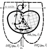
Figure VIII.1: Only Containment: Pursuer cannot follow all the variations of the evader

Definition 47.

Let $\mathcal{L}_{e}({\bf e_{0}},T)$ be a $CSE$. Let $\mathcal{L}_{e}^{-}({\bf e_{0}},R_{p}^{c},T-\delta)\neq\emptyset$ for all $\delta>0$ and for all $R_{p}^{c}({\bf p_{0}},T-\delta)\in\mathfrak{R}_{p}$. Let $\mathcal{C}_{p}({\bf p_{0}},T)$ be a $CSP$ such that $\mathcal{L}_{e}^{-}({\bf e_{0}},\mathcal{C}_{p},T)=\emptyset$. We call the $\mathcal{L}_{e}({\bf e_{0}},T)$ the last $CSE$ ($LCSE$) and $\mathcal{C}_{p}({\bf p_{0}},T)$ as capturing $CSP$ ($CCSP$). Note that a pair of a $LCSE$ and a $CCSP$ is not unique.

Theorem 48.

Let $T$ be as defined by (V). For every pursuer trajectory ${\bf p}$ corresponding to feedback policy ${\bf u_{p}}\in\mathcal{U}_{p}$ there exists an evader trajectory ${\bf e}$ corresponding to feedback strategy ${\bf u_{e}}\in\mathcal{U}_{e}$ s.t. ${\bf e}_{|\mathbb{R}^{2}}(t)\neq{\bf p}_{|\mathbb{R}^{2}}(t)$ for all $t<T$

Proof:

This situation can be divided into two cases:

Case 1: Consider a time instant $\tilde{t}<T$ such that $\mathcal{L}_{e}^{-}({\bf e_{0}},R_{p}^{c},\tilde{t})\neq\emptyset$ for all $R_{p}^{c}({\bf p_{0}},\tilde{t})\in\mathfrak{R}_{p}$ and $R_{e}^{-}({\bf e_{0}},R_{p},\tilde{t})\neq\emptyset$ for $R_{p}({\bf p_{0}},\tilde{t})$. Since $R_{e}^{-}({\bf e_{0}},R_{p},\tilde{t})\neq\emptyset$, there exists an evader strategy ${\bf u_{e}}\in\mathcal{U}_{e}$ such that ${\bf e}_{|\mathbb{R}^{2}}(t)\notin R_{p}({\bf p}_{0},t)$ for each $t\leq\tilde{t}$. Thus the evader can always escape capture at each $t\leq\tilde{t}$.

Case 2: Consider a time instant $\hat{t}<T$ such that $\mathcal{L}_{e}^{-}({\bf e_{0}},R_{p}^{c},\hat{t})\neq\emptyset$ for all $R_{p}^{c}({\bf p_{0}},\hat{t})\in\mathfrak{R}_{p}$ but $R_{e}^{-}({\bf e_{0}},R_{p},\hat{t})=\emptyset$. Since $R_{e}^{-}({\bf e_{0}},R_{p},\hat{t})=\emptyset$, every trajectory ${\bf e}$ of the evader, corresponding to open loop input ${\bf u_{e}}$, can be intercepted by some pursuer strategy ${\bf p}$ corresponding to a suitable pursuer input ${\bf u_{p}}$. This is shown in Figure VIII.1 where the solid curve (labeled ${\bf e}$) denotes an evader trajectory ${\bf e}_{|\mathbb{R}^{2}}$ and the solid curve (labeled ${\bf p}$) denotes the pursuer trajectory ${\bf p}_{|\mathbb{R}^{2}}$. Let the pursuer strategy ${\bf p}$ intercept the evader, using the input ${\bf u_{e}}$, at a point ${\bf c}\in\mathcal{L}_{e}({\bf e_{0}},\hat{t})$. Since, $\mathcal{L}_{e}^{-}({\bf e_{0}},R_{p}^{c},\hat{t})\neq\emptyset$ $\forall$ $R_{p}^{c}({\bf p_{0}},\hat{t})\in\mathfrak{R}_{p}$, $\exists$ a curve $\overline{{\bf x}{\bf y}}\in\mathcal{L}_{e}({\bf e_{0}},\hat{t})$ (depicted by the solid curve from ${\bf x}$ to ${\bf y}$ in Figure VIII.1 ) which is not a continuum set for the pursuer. Extend the curve $\overline{{\bf xy}}$ from point ${\bf x}$ to ${\bf c}\in\mathcal{L}_{e}({\bf e_{0}},\hat{t})$ by a curve $\overline{{\bf xc}}\in\mathcal{L}_{e}({\bf e_{0}},\hat{t})$. Call the new curve $\overline{{\bf cy}}$. Since the curve ${\bf\overline{xy}}\in\mathcal{L}_{e}^{-}({\bf e_{0}},R_{p}^{c},\hat{t})$ is not a continuum set for the pursuer, the curve ${\bf\overline{cy}}$ is also not a continuum set for the pursuer. However, the curve ${\bf\overline{cy}}\in\mathcal{L}_{e}^{-}({\bf e_{0}},R_{p}^{c},\hat{t})$ is a continuum set for the evader. Thus the evader with a variation $\delta{\bf u_{e}}$ in its strategy can change the end point to ${\bf y}$ from point ${\bf c}$ (The evader trajectory corresponding to input ${\bf u_{e}+\delta u_{e}}$ is shown by a dashed curve and labeled ${\bf e}+\delta{\bf e}$ ). However, since ${\bf\overline{cy}}$ is not a continuum set for the pursuer, the pursuer cannot catch the evader in time $\hat{t}$ using an admissible variation $\delta{\bf u_{p}}$. Thus the evader can always avoid capture for all time $t\leq\hat{t}<T$. ∎

Proof of Theorem 29: By Theorem 48, in order to maximize the time-to-capture the evader should use input strategy ${\bf u_{e}^{*}}\in\mathcal{U}_{e}$ such that, ${\bf e}_{|\mathbb{R}^{2}}(T)={\bf z}\in\mathcal{L}_{e}({\bf e_{0}},T)$, and ${\bf e}_{|\mathbb{R}^{2}}(t)\notin\mathcal{C}_{p}({\bf p_{0}},t)$ $\forall$ $t<T$. On the other hand, the pursuer should use time-optimal input strategy ${\bf u_{p}^{*}}\in\mathcal{U}_{p}$ such that ${\bf p}_{|\mathbb{R}^{2}}(T)={\bf z}$ and ${\bf p}_{|\mathbb{R}^{2}}(t)\in\mathcal{C}_{p}({\bf p_{0}},T)$ $\forall\ t\leq T$ in order to minimize the time to capture the evader. Thus if the evader uses ${\bf u_{e}^{*}}\in\mathcal{U}_{e}$ and pursuer uses ${\bf u_{p}^{*}}\in\mathcal{U}_{p}$ the time to capture $T_{c}({\bf u_{p}^{*}},{\bf u_{e}^{*}})=T$. If the evader deviates from ${\bf u_{e}^{*}}$ by ${\bf\delta u_{e}}$ then by Theorem 46 it will be captured at $T_{c}({\bf u_{p}^{*}},{\bf u_{e}^{*}}+{\bf\delta u_{e}})\leq T$. Similarly, if the pursuer deviates from ${\bf u_{p}^{*}}$ by ${\bf\delta u_{p}}$ it will not be able to reach point ${\bf e}_{|\mathbb{R}^{2}}(T)={\bf z}\in\mathcal{C}_{p}({\bf e_{0}},T)$ at time $T$ and we have $T\leq T_{c}({\bf u_{p}^{*}}+{\bf\delta u_{p}},{\bf u_{e}^{*}})$. Thus,

$$T_{c}({\bf u_{p}^{*}},{\bf u_{e}^{*}}+{\bf\delta u_{e}})\leq T=T_{c}({\bf u_{p}^{*}},{\bf u_{e}^{*}})\leq T_{c}({\bf u_{p}^{*}}+{\bf\delta u_{p}},{\bf u_{e}^{*}})$$ (VIII.1)

and hence ${\bf u_{e}^{*}}$ and ${\bf u_{p}^{*}}$ are the feedback saddle-point strategies. Since, $T$ satisfies (VIII.1) we have $T=T^{*}$.

IX Proof of Theorem 30

In this section we explicitly characterize the continuous subset of evader’s reachable set which will be the $LCSE$. For the pursuer we show that $CCSP$ will be a set from among three particular continuous subsets of the pursuer’s reachable set. Using $LCSE$ and $CCSP$ we show that the saddle point trajectories are of the type $CS$.

IX-A Characterization of $LCSE$

In this section we characterize the $LCSE$ $\mathcal{L}_{e}({\bf e_{0}},T^{*})$. Recall that $r_{p}$ and $r_{e}$ are the minimum turning radii of the pursuer and the evader respectively, while $d_{pe}^{0}$ denotes the initial distance between the pursuer and the evader. If the capture time $T^{*}\geq 2\pi r_{e}/v_{e_{m}}$, then we show that the boundary of $LCSE$ is the external boundary of evader’s reachable set. This simplifies the analysis of the game significantly. Hence, in order to ensure that the capture of evader takes at least time $2\pi r_{e}/v_{e_{m}}$ we add an assumption on the initial distance between the pursuer and the evader.

Lemma 49.

If $d_{pe}^{0}\geq 2r_{e}+2\pi r_{e}(v_{p_{m}}/v_{e_{m}})$ then capture can occur only at time $t\geq 2\pi r_{e}/v_{e_{m}}$.

Proof:

Let the evader be located at $E$, at a distance $d_{pe}^{0}$ away from the pursuer located at $P$, as shown in Figure IX.1. Let $PA$ be the line from pursuer’s position to the center of anti-clockwise evader circle denoted by point $A$. Also, let $PA$ intersect the anticlockwise circle at point $O$. The least time for the pursuer to reach point $O$ is

$$t_{m}:=\text{len}(PO)/v_{p_{m}}=(\text{len}(PA)-r_{e})/v_{p_{m}}$$ (IX.1)

Also from triangle inequality we have $\text{len}(PA)\geq\text{len}(PE)-r_{e}$. Thus (IX.1) becomes

$$t_{m}\geq(\text{len}(PE)-r_{e}-r_{e})/v_{p_{m}}=[d_{pe}^{0}-2r_{e}]/v_{p_{m}}$$

Let, $t_{p}:=(d_{pe}^{0}-2r_{e})/v_{p_{m}}$ and $t_{e}:=2\pi r_{e}/v_{e_{m}}$. Thus if $t_{p}\geq t_{e}$ the pursuer requires at least $t_{e}$ time to reach any point on evader circles. Thus the evader, by using $v_{e}(t)=0$ and $u_{e}(t)=0$ $\forall\ t$ can avoid capture up to time $t_{e}$ (since it remains at point $E$ $\forall\ t$ and pursuer takes at least time $t_{e}$ to reach it). Further, if it uses time optimal evasion strategy then the time to capture will certainly be greater than $t_{e}$. Thus, if $d_{pe}^{0}\geq 2r_{e}+2\pi r_{e}(v_{p_{m}}/v_{e_{m}})$ we have $t_{p}=(d_{pe}^{0}-2r_{e})/v_{p_{m}}\geq 2\pi r_{e}/v_{e_{m}}$. This implies $t_{p}\geq t_{e}$ and the claim follows. ∎

Figure IX.1: Evader capture after $t\geq 2\pi r_{e}/v_{e_{m}}$

Recall that, by Lemma 39, the central reachable set $R_{e}^{CR}({\bf e_{0}},T^{*})$ is a $CSE$. In next theorem we prove that the $LCSE$ is in fact $R_{e}^{CR}({\bf e_{0}},T^{*})$ if $d_{pe}^{0}\geq 2r_{e}+2\pi r_{e}(v_{p_{m}}/v_{e_{m}})$. Further, since the boundary of $R_{e}^{CR}({\bf e_{0}},T^{*})$ and the external boundary of $R_{e}({\bf e_{0}},T^{*})$ are the same, it follows that the whole reachable set of the evader must be contained in some continuous subset of the evader’s reachable set. In the next theorem we specialize the Theorems 46 and 48 for the assumption that $d_{pe}^{0}\geq 2r_{e}+2\pi r_{e}(v_{p_{m}}/v_{e_{m}})$, and give a necessary and sufficient condition for capture under feedback trajectories.

Theorem 50.

Let $d_{pe}^{0}\geq 2r_{e}+2\pi r_{e}(v_{p_{m}}/v_{e_{m}})$. For every evader trajectory ${\bf e}_{|\mathbb{R}^{2}}$ generated by feedback policy ${\bf u_{e}}\in\mathcal{U}$ there exists a pursuer trajectory ${\bf p}_{|\mathbb{R}^{2}}$ corresponding to feedback strategy ${\bf u_{p}}\in\mathcal{U}_{p}$ s.t. ${\bf e}_{|\mathbb{R}^{2}}(t)={\bf p}_{|\mathbb{R}^{2}}(t)$ for some $t\leq T^{*}$ if and only if $R_{e}^{-}({\bf e_{0}},\mathcal{C}_{p},T^{*})=\emptyset$ for a $CCSP$ $\mathcal{C}_{p}({\bf p_{0}},T^{*})$.

Proof:

First we show the $only\ if$ part. As seen in Lemma 49, if $d_{pe}^{0}\geq 2r_{e}+2\pi r_{e}(v_{p_{m}}/v_{e_{m}})$ the pursuer can capture the evader only after time $t_{e}=2\pi r_{e}/v_{e_{m}}$. The evader’s central reachable set after time $t\geq t_{e}=2\pi r_{e}/v_{e_{m}}$ is shown in Figure VII.3. It can be easily seen that the external boundary of the evader’s reachable set and that of the central reachable set are the same i.e. $\partial R_{e}({\bf e_{0}},T^{*})=\partial R_{e}^{CR}({\bf e_{0}},T^{*})$. Now, $R_{e}^{CR}({\bf e_{0}},T^{*})$ is a $CSE$. By Theorems 48 and 46 $R_{e}^{CR}({\bf e_{0}},T^{*})$ must be contained inside some $CCSP$ $\mathcal{C}_{p}({\bf p_{0}},T^{*})$ for capture to occur at time $t\leq T^{*}$. Since, $\partial R_{e}({\bf e_{0}},T^{*})=\partial R_{e}^{CR}({\bf e_{0}},T^{*})$, it is necessary that $R_{e}({\bf e_{0}},T^{*})$ must be contained inside some $\mathcal{C}_{p}({\bf p_{0}},T^{*})$ for the capture to occur at $t\leq T^{*}$.

Now we prove the $if$ part. Since $R_{e}^{c}({\bf e_{0}},T^{*})\subseteq R_{e}({\bf e_{0}},T^{*})$ for all $R_{e}^{c}({\bf e_{0}},T^{*})\in\mathfrak{R}({\bf e_{0}},T^{*})$, the condition $R_{e}^{-}({\bf e_{0}},\mathcal{C}_{p},T^{*})=\emptyset$ implies that every $R_{e}^{c}({\bf e_{0}},T^{*})$$\in$$\mathfrak{R}_{e}({\bf e_{0}},T^{*})$ is such that $R_{e}^{c-}({\bf e_{0}},\mathcal{C}_{p},T^{*})=\emptyset$ for some corresponding $CCSP$ $\mathcal{C}_{p}({\bf p_{0}},T^{*})$. Thus by Theorems 46 and 48 we can conclude that capture will occur at $t\leq T^{*}$. ∎

IX-B Characterization of $CCSP$

Next, we will characterize $CCSP$ $\mathcal{C}_{p}({\bf p_{0}},T^{*})$ in order to determine the nature of feedback strategies. We will show that the $CCSP$ is either the blocking set $B_{p}({\bf p_{0}},{\bf e_{0}},T^{*})$ or the truncated left reachable set $R_{p}^{l_{t}}({\bf p_{0}},T^{*})$ or the truncated right reachable set $R_{p}^{r_{t}}({\bf p_{0}},T^{*})$. First we define the concept of blocking $LS$ and $RS$ trajectories of the pursuer.

Definition 51.

Blocking trajectory of the pursuer : If the initial position of the evader (${\bf e_{0}}$) and pursuer (${\bf p_{0}}$) is such that all the points on a pursuer trajectory are reached by the pursuer earlier than the evader then we say that such a trajectory is a blocking trajectory. Further, if the blocking trajectory is of the type $LS\ (RS)$ then we call it $LS\ (RS)$ blocking trajectory.

This concept of blocking trajectory will be used to analyze the containment of evader’s reachable set by $B_{p}({\bf p_{0}},{\bf e_{0}},T^{*})$, $R_{p}^{l_{t}}({\bf p_{0}},T^{*})$, and $R_{p}^{r_{t}}({\bf p_{0}},T^{*})$.

Continuous capture by blocking set

We show that the blocking set (defined in Definition 43 and shown to be a continuous subset in Lemma 44) will contain the evader’s reachable set for all initial conditions of the pursuer and the evader such that $d_{pe}^{0}\geq 2r_{e}+2\pi r_{e}(v_{p_{m}}/v_{e_{m}})$. Recall that $\tilde{T}_{l}^{v}$ and $\tilde{T}_{r}^{v}$ are the trajectories of the type $LS$ and $RS$ as defined in Definition 43. The next lemma follows easily from the construction of $B_{p}({\bf p_{0}},{\bf e_{0}},\bar{t})$ for some time $\bar{t}\geq 2\pi r_{p}/v_{p_{m}}$.

Lemma 52.

$\tilde{T}_{l}^{v}$ is a blocking $LS$ trajectory while $\tilde{T}_{r}^{v}$ is a blocking $RS$ trajectory if $d_{pe}^{0}\geq 2r_{e}+2\pi r_{e}(v_{p_{m}}/v_{e_{m}})$.

Remark 53.

By Lemma 52, $\tilde{T}_{l}^{v}$ and $\tilde{T}_{r}^{v}$ block the evader from entering the region shown by crisscross shading in Figure IX.4. Some examples of blocking sets have been shown in Figures IX.4, IX.10, and IX.7. As can be seen from these examples, at most one curve out of $\tilde{T}_{l}^{v}$ and $\tilde{T}_{r}^{v}$ can end on the left internal boundary or the right internal boundary for any position of the pursuer and evader after time $\bar{t}\geq 2\pi r_{p}/v_{p_{m}}$.

Next we show that for all possible initial positions of the evader, the blocking set will contain the evader’s reachable set at some time $T_{b}<\infty$.

Lemma 54.

For every evader and pursuer initial positions such that $d_{pe}^{0}\geq 2r_{e}+2\pi r_{e}(v_{p_{m}}/v_{e_{m}})$, the set $R_{e}^{-}({\bf e_{0}},B_{p},T_{b})=\emptyset$ for some time $T_{b}<\infty$.

Proof:

Recall that, if $d_{pe}^{0}\geq 2r_{e}+2\pi r_{e}(v_{p_{m}}/v_{e_{m}})$ then each of the left reachable set and the right reachable set contain the evader’s reachable set at times $T_{l}$ and $T_{r}$ respectively (by Lemma 17 and Lemma 18). Now, since either the blocking curve $\tilde{T}_{l}^{v}$ or the blocking curve $\tilde{T}_{r}^{v}$ may end on the internal boundary, without loss of generality, let $\tilde{T}_{l}^{v}$ end on the left internal boundary (see Definition 14) as shown in Figure IX.4. Now consider the left reachable set of the pursuer. Some portion of the left reachable set is not a part of the blocking set. Thus, at time $t_{m}=\max(T_{l},T_{r})$, $B_{p}({\bf p_{0}},{\bf e_{0}},t_{m})$ may not contain some part of $R_{e}({\bf e_{0}},t_{m})$ even if the left reachable set contains the reachable set completely. However, since $d_{pe}^{0}\geq 2r_{e}+2\pi r_{e}(v_{p_{m}}/v_{e_{m}})$ the evader cannot enter this part as $\tilde{T}_{l}^{v}$ and $\tilde{T}_{r}^{v}$ are blocking curves (by Lemma 52). Apart from this portion the left reachable set is a part of $B_{p}({\bf p_{0}},{\bf e_{0}},t_{m})$. Thus, the remaining part of $R_{e}({\bf e_{0}},t_{m})$ is contained in the blocking set and we have $R_{e}^{-}({\bf e_{0}},B_{p},t_{m})=\emptyset$. Hence, for some time $T_{b}\leq t_{m}$ we will have $R_{e}^{-}({\bf e_{0}},B_{p},T_{b})=\emptyset$ . ∎

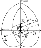
Figure IX.2: Construction of $B_{p}({\bf p_{0}},{\bf e_{0}},\bar{t})$

Figure IX.3: $B_{p}({\bf p_{0}},{\bf e_{0}},\bar{t})$: Evader behind on left side (shaded region)

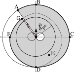
Figure IX.4: $B_{p}({\bf p_{0}},{\bf e_{0}},\bar{t})$: Evader behind on right side (shaded region)

Continuous containment by truncated left reachable set

In this section we analyze the conditions under which $R_{p}^{l_{t}}({\bf p_{0}},\bar{t})$ and $R_{p}^{r_{t}}({\bf p_{0}},\bar{t})$ can contain the evader’s reachable set at some time $\bar{t}$. First we define two $LS$ ($RS$) blocking trajectories for the truncated left (right) reachable set.

Let $PA$ be the curve defined by (III.1) with $t_{1}=0$ and is shown in Figure III.4. We call this curve $BL^{1}$. Similarly, let $PCB$ be the curve defined by (III.1) with $t_{1}=2\pi r_{p}/v_{p_{m}}$ and is shown in Figure III.4. We call this curve $BL^{2}$. Analogously, $BR^{1}$ and $BR^{2}$ are defined for the truncated right reachable set.

Remark 55.

Now, the left reachable set $R_{p}^{l}({\bf p_{0}},T_{l})$ contains the evader’s reachable set at time $T_{l}$ (by Lemma 17). Since the truncated reachable set does not contain $PA$ and the anti-clockwise circle $A_{p}(0)$, hence if evader’s reachable set intersects the line $PA$ or the anti-clockwise circle, continuous containment by $R_{p}^{l}({\bf p_{0}},T_{l})$ will not happen. However, such a situation is avoided since $BL^{1}$ and $BL^{2}$ act as blocking curves for some initial conditions of the pursuer and the evader, and block the evader from entering the points in $PA$ and $A_{p}(0)$ analogous to what $\tilde{T}_{l}^{v}$ and $\tilde{T}_{r}^{v}$ achieve for the blocking set. This is shown in Proposition 61.

First we define some terminology. Consider Figure IX.7. Let $OPQ$ be the line passing through the pursuer position $P$ and perpendicular to the orientation of the pursuer. If the evader is in the closed half plane in the direction opposite to the orientation of the pursuer then we say that the evader is behind the pursuer. If the evader is located in the open half plane in the direction of the orientation of the pursuer then we say that the evader is located in the front of the pursuer. For $R_{p}^{l_{t}}({\bf p_{0}},T_{l})$, let $PF$ be the line as shown in Figure IX.7 at an angle $\theta$ with respect to $PS$. The shaded region between $PO$ and $PF$, for $\theta=\arccos\left(2\pi r_{p}v_{e_{m}}/(v_{p_{m}}d_{pe}^{0})\right)$, is denoted by $S^{l}(T_{l})$. Similarly, for $R_{p}^{r_{t}}({\bf p_{0}},T_{r})$ let $PF$ be the line as shown in Figure IX.7 at an angle $\theta$ with respect to $PS$. The shaded region between $PO$ and $PF$ for, $\theta=\arccos\left(2\pi r_{p}v_{e_{m}}/(v_{p_{m}}d_{pe}^{0})\right)$, is denoted by $S^{r}(T_{r})$.

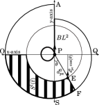
Figure IX.5: $BL^{2}$: Blocking $LS$ trajectory

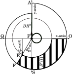
Figure IX.6: $BR^{2}$: Blocking $RS$ trajectory

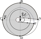
Figure IX.7: $B_{p}({\bf p_{0}},{\bf e_{0}},T_{b})$ as active set

Lemma 56.

Let $d_{pe}^{0}\geq 2r_{e}+2\pi r_{e}(v_{p_{m}}/v_{e_{m}})$ and let the evader’s initial position be in $S^{l}(T_{l})$. Then, $R_{p}^{l_{t}}({\bf p_{0}},T_{l})$ will contain the evader’s reachable set continuously.

Proof:

$BL^{1}$ as blocking trajectory : Since evader is in $S^{l}(T_{l})$, it is behind the pursuer. All the points on the trajectory $BL^{1}$ can be reached by the pursuer before the evader can reach them. Hence, it becomes the blocking $LS$ trajectory. Thus $BL^{1}$ will prevent the evader from reaching any point on $PA$ from the left side of the pursuer.

$BL^{2}$ as blocking trajectory : If $d_{pe}^{0}\geq 2r_{e}+2\pi r_{e}(v_{p_{m}}/v_{e_{m}})$ then the pursuer can reach all the points on the anti-clockwise circle of the pursuer before the evader (This follows from analysis similar to Lemma 49). Since the boundary of $A_{p}(0)$ forms a part of $BL^{2}$ we can conclude that $BL^{2}$ prevents the evader from entering $A_{p}(0)$.

Now, if the evader tries to reach any point on line $PA$ from the right, while the pursuer is initially traveling on $A_{p}(0)$, we will show that $BL^{2}$ will intercept the evader. If the pursuer follows $BL^{2}$, it will reach point $P$ again after encircling the anticlockwise circle once, for which it will require time $t_{p}:=2\pi r_{p}/v_{p_{m}}$. Thus if the evader requires time $t_{e}\geq t_{p}$ to reach the line $OPQ$ then $BL^{2}$ will be a blocking $LS$ trajectory. Let the evader be located at an angle $\theta$ with respect to line $PS$ as shown in Figure IX.7. At this position the evader requires minimum time to reach a point on line $OPQ$ if it is pointing upwards. This minimum time is $d_{pe}^{0}\cos(\theta)/v_{e_{m}}$. Thus $t_{e}\geq d_{pe}^{0}\cos(\theta)/v_{e_{m}}$. Hence $BL^{2}$ is the blocking trajectory if

$$d_{pe}^{0}\cos(\theta)/v_{e_{m}}\geq 2\pi r_{p}/v_{p_{m}};\quad\cos(\theta)\geq 2\pi r_{p}v_{e_{m}}/(v_{p_{m}}d_{pe}^{0})$$

This implies that for $\theta\leq\arccos\left(2\pi r_{p}v_{e_{m}}/(v_{p_{m}}d_{pe}^{0})\right)$, $BL^{2}$ will act as blocking trajectory.

The left reachable set contains the evader’s reachable set at time $T_{l}$ (by Lemma 17). Further, $BL^{1}$ and $BL^{2}$ act as blocking curves and block the evader from entering the points in $PA$ and $A_{p}(0)$ and the claim follows. ∎

Definition 57.

Let $T_{l}^{c}$ be the minimum time such that $R_{e}({\bf e_{0}},T_{l}^{c})\subseteq R_{p}^{l_{t}}({\bf p_{0}},T_{l}^{c})$ continuously i.e. $R_{e}^{-}({\bf e_{0}},R_{p}^{l_{t}},T_{l}^{c})=\emptyset$. If for some initial positions of the pursuer and the evader, $R_{p}^{l_{t}}({\bf p_{0}},T_{l}^{c})$ does not contain $R_{e}({\bf e_{0}},T_{l}^{c})$ continuously then we say $R_{e}^{-}({\bf e_{0}},R_{p}^{l_{t}},T_{l}^{c})=\emptyset$ at $T_{l}^{c}=\infty$.

Remark 58.

From the above analysis it follows that if $T_{l}^{c}<\infty$ then $T_{l}^{c}=T_{l}$. However, if $T_{l}^{c}=\infty$ this implies that the truncated left reachable set cannot contain evader’s reachable set continuously.

Lemma 59.

Let $d_{pe}^{0}\geq 2r_{e}+2\pi r_{e}(v_{p_{m}}/v_{e_{m}})$ and let the evader’s initial position be located in $S^{r}(T_{r})$. Then, $R_{p}^{r_{t}}({\bf p_{0}},T_{r})$ will contain the evader’s reachable set continuously at some finite time $\bar{t}\geq 2\pi r_{p}/v_{p_{m}}$.

Remark 60.

The minimum time for continuous containment by the truncated right reachable set is denoted by $T_{r}^{c}$. If $T_{r}^{c}<\infty$ then $T_{r}^{c}=T_{r}$. However, if $T_{r}^{c}=\infty$ this implies that the truncated right reachable set cannot contain evader’s reachable set continuously.

Proposition 61.

Let $d_{pe}^{0}\geq 2r_{e}+2\pi r_{e}(v_{p_{m}}/v_{e_{m}})$. If the evader is behind the pursuer then the evader’s reachable set is contained continuously in the left reachable set or the right reachable set or both at time $t_{lr}=\min(T_{l}^{c},T_{l}^{r})$.

Proof:

If the evader is behind the pursuer at a distance greater than $d_{pe}^{0}\geq 2r_{e}+2\pi r_{e}(v_{p_{m}}/v_{e_{m}})$ it is either located in $S^{l}(T_{l}^{c})$ or $S^{r}(T_{r}^{c})$ or both and the claim follows from Lemma 56 and Lemma 59. ∎

Representative set and frontier boundaries

Next, we define the representative set at time $t\geq 2\pi r_{p}/v_{p_{m}}$ which comprises of the blocking set, truncated left reachable set, and the truncated right reachable set.

Definition 62.

Representative set at time $t\geq 2\pi r_{p}/v_{p_{m}}$ is

$$\mathfrak{R}({\bf p_{0}},{\bf e_{0}},t): = \{B_{p}({\bf p_{0}},{\bf e_{0}},t),R_{p}^{l_{t}}({\bf p_{0}},t),R_{p}^{r_{t}}({\bf p_{0}},t)\}$$

Let $T_{a}$ be the time such that for some $\tilde{R}_{p}^{c}\in\mathfrak{R}({\bf p_{0}},{\bf e_{0}},T_{a})$ we have $R_{e}^{-}({\bf e_{0}},\tilde{R}_{p}^{c},T_{a})=\emptyset$ and for all $t<T_{a}$, $R_{e}^{-}({\bf e_{0}},R_{p}^{c},t)\neq\emptyset$ for all $R_{p}^{c}\in\mathfrak{R}({\bf p_{0}},{\bf e_{0}},t)$ i.e. $T_{a}=\min\{T_{b},T_{l}^{c},T_{r}^{c}\}$. We denote this set $\tilde{R}_{p}^{c}\in\mathfrak{R}({\bf p_{0}},{\bf e_{0}},T_{a})$ by $\mathcal{A}_{p}(T_{a})$ and call it the active pursuer set.

Note that, since $R_{e}^{-}({\bf e_{0}},B_{p},T_{b})=\emptyset$ for some time $T_{b}<\infty$ (Lemma 54), we have $T_{a}<\infty$.

Remark 63.

The capture criterion, which could not be explained using only containment of reachable sets can now be explained using the active set and $LCSE$. Consider the position of the pursuer and evader as shown in the Figure IV.3. In this case the active set is the left reachable set as shown in Figure IX.13 and capture occurs at time $T_{l}^{c}=T_{l}$. Further, at time $t<T_{l}$, the safe region of evader is non-empty (shown in Figure IX.13). Next consider the situation when the evader is located ahead of the pursuer as shown in Figure IV.3. In this case the blocking set is the active set. The capture is shown in Figure IX.10 and occurs at time $T_{b}$. For any time $t<T_{b}$ the safe region of the evader is non-empty (as shown in Figure IX.10) and the evader can escape capture using feedback strategies. In the above examples the active set explains capture under feedback strategies. In fact, we will show that if the evader is in front of the pursuer then it suffices to consider blocking set as $CCSP$ and if the evader is behind the pursuer then it suffices to consider either the left reachable set or the right reachable set as $CCSP$.

Next we define frontier boundary for all the sets in the representative set.

Definition 64.

Frontier boundary:

1. The frontier boundary of $R_{p}^{l_{t}}({\bf p_{0}},t)$ is the portion of the external boundary denoted by $ADEFB$ (start point $A$ to end point $B$) as shown in Figure III.4 by dashed curve i.e. we exclude the portion $BA$ from $\partial R_{p}^{l}({\bf p_{0}},t)$.

2. The frontier boundary of $R_{p}^{r_{t}}({\bf p_{0}},t)$ is defined analogously.

3. The frontier boundary of the blocking set is the portion of external boundary of the blocking set excluding the blocking curves $\tilde{T}_{l}^{v}$ and $\tilde{T}_{r}^{v}$. For example, the frontier boundary of blocking set in Figure IX.4 is denoted by $ABCDFG$.

Remark 65.

The frontier boundaries of all the sets expand outwards radially with time. Also the external boundary of the evader reachable set expands out radially. As a result, for the active set, the capture occurs on the frontier boundary.

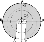
Figure IX.8: $B_{p}({\bf p_{0}},{\bf e_{0}},t_{m})$: Evader in front (shaded region)

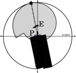
Figure IX.9: Active Set: Blocking set

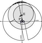
Figure IX.10: Evader safe region

Next we demonstrate that if $d_{pe}^{0}\geq 2r_{e}+2\pi r_{e}(v_{p_{m}}/v_{e_{m}})$ the evader can always escape capture for all time $t<T_{a}$. We do this in by considering a particular set in representative set to be a active set in the Propositions 66, 67, and 71.

Proposition 66.

Let $d_{pe}^{0}\geq 2r_{e}+2\pi r_{e}(v_{p_{m}}/v_{e_{m}})$. If $\mathcal{A}_{p}(T_{a})=R_{p}^{l_{t}}({\bf p_{0}},T_{a})$ and $T_{a}=T_{l}^{c}<\infty$, then the evader can always escape capture for $t<T_{a}$ by using feedback strategy.

Proof:

First we divide the frontier boundary of $R_{p}^{l_{t}}({\bf p_{0}},T_{a})$ into two parts $ADE$ and $EGFHB$ as shown in Figure IX.13. Let ${\bf z}\in\mathbb{R}^{2}$ be a last point of $R_{e}({\bf e_{0}},T_{a})$ covered by $R_{p}^{l_{t}}({\bf p_{0}},T_{a})$ at time $T_{a}$. Since the frontier boundary of $R_{p}^{l_{t}}({\bf p_{0}},t)$ and the external boundary $R_{e}({\bf e_{0}},t)$ both grow out radially with time $t$, ${\bf z}$ will lie on the external boundary of $R_{e}({\bf e_{0}},T_{a})$. Also, the point in $R_{p}^{l_{t}}({\bf p_{0}},T_{a})$ which covers ${\bf z}$ will lie on the frontier boundary of $R_{p}^{l_{t}}({\bf p_{0}},T_{a})$. Now the situation can be divided into two cases:

Case 1: Let ${\bf z}\in ADE$. Then at time $T_{a}^{\prime}<T_{a}$ we have $R_{e}^{-}({\bf e_{0}},R_{p}^{l},T_{a}^{{}^{\prime}})\neq\emptyset$ i.e. the pursuer’s reachable set does not cover the evader’s reachable set and the evader can always escape capture.

Case 2: Let ${\bf z}\in EGFHB$. We further divide the portion $EGFHB$ into two parts namely $EGF$ and $FHB$ as shown in Figure IX.13. Now let ${\bf z}\in FHB$. In Figure IX.13 the right reachable set is shown by dotted curve. Since $d_{pe}^{0}\geq 2r_{e}+2\pi r_{e}(v_{p_{m}}/v_{e_{m}})$, the evader is located outside the circle of radius $d_{pe}^{0}$. It is clear from geometry that if ${\bf z}\in FHB$ then the right external boundary would have covered the evader’s reachable set earlier. Thus the right reachable set would have been the active set and this contradicts the assumption that $R_{p}^{l_{t}}({\bf p_{0}},T_{a})$ is the active set.

Next, let ${\bf z}\in EGF$. Let $T_{a}^{{}^{\prime}}<T_{a}$ s.t. $R_{e}^{-}({\bf e_{0}},R_{p},T_{a}^{{}^{\prime}})=\emptyset$ ( If $R_{e}^{-}({\bf e_{0}},R_{p},T_{a}^{{}^{\prime}})$$\neq\emptyset$ then the pursuer’s reachable set does not cover the evader’s reachable set and the evader can always escape capture). At time $T_{a}^{{}^{\prime}}$, $R_{p}^{l_{t}}({\bf p_{0}},T_{a}^{{}^{\prime}})$ will not cover evader’s reachable set completely. Since $R_{e}^{-}({\bf e_{0}},R_{p},T_{a}^{{}^{\prime}})=\emptyset$, this uncovered region must form a part of the right reachable set of the pursuer. Further, there must exist a point ${\bf x}$ in the evader’s reachable set such that ${\bf x}\in\left[R_{p}^{l_{t}}({\bf p_{0}},T_{a}^{{}^{\prime}})\backslash R_{p}^{r_{t}}({\bf p_{0}},T_{a}^{{}^{\prime}})\right]\cap R_{e}({\bf e_{0}},T_{a}^{{}^{\prime}})$. (For if such a point does not exist then the evader’s reachable set at $T_{a}^{{}^{\prime}}$ would be entirely contained by the the right reachable set. Since, $R_{p}^{r_{t}}({\bf p_{0}},T_{a}^{{}^{\prime}})$ is in the representative set this would contradict the assumption that $R_{p}^{l_{t}}({\bf p_{0}},T_{a})$ is the active set). Also, there exists a point ${\bf y}\in\left[R_{p}^{r_{t}}({\bf p_{0}},T_{a}^{{}^{\prime}})\backslash R_{p}^{l_{t}}({\bf p_{0}},T_{a}^{{}^{\prime}})\right]\cap R_{e}({\bf e_{0}},T_{a}^{{}^{\prime}})$ (Otherwise we would have $R_{e}^{-}({\bf e_{0}},R_{p}^{l},T_{a}^{{}^{\prime}})=\emptyset$ and this will contradict the assumption that the minimum time at which $R_{e}^{-}({\bf e_{0}},R_{p}^{l_{t}},t)=\emptyset$ is $T_{a}$ since $T_{a}^{{}^{\prime}}<T_{a}$). Now consider a curve ${\bf\overline{xy}}$ in the evader’s reachable set as shown in Figure VII.3. Since ${\bf z}\in EGF$, such a curve is behind the pursuer and as shown in the proof of Lemma 45 it is not a continuum curve for the pursuer. Hence, at time $T_{a}^{{}^{\prime}}<T_{a}$, $R_{e}^{-}({\bf e_{0}},R_{p}^{c},T_{a}^{{}^{\prime}})\neq\emptyset$ for all $CSP$ $R_{p}^{c}({\bf p_{0}},T_{a}^{{}^{\prime}})$ and the evader can escape capture. ∎

Figure IX.11: Left reachable set as active set

Figure IX.12: Continuous containment by left reachable set

Figure IX.13: Safe region: Continuous containment by left reachable set

The proof of Proposition 67 is similar to that of Proposition 66.

Proposition 67.

Let $d_{pe}^{0}\geq 2r_{e}+2\pi r_{e}(v_{p_{m}}/v_{e_{m}})$. If $\mathcal{A}_{p}(T_{a})=R_{p}^{r_{t}}({\bf p_{0}},T_{a})$ and $T_{a}=T_{r}^{c}<\infty$, then evader can always escape capture for $t<T_{a}$ by using feedback strategy.

Remark 68.

Consider a situation where the active set is the blocking set and either the truncated left reachable set or the truncated right reachable set contains the evader’s reachable set continuously. In such a situation either the truncated left reachable set or the truncated right reachable set is also an active set along with the blocking set. This is established in the next lemma.

Lemma 69.

Let $T_{lr}=\min(T_{l}^{c},T_{r}^{c})$ and $d_{pe}^{0}\geq 2r_{e}+2\pi r_{e}(v_{p_{m}}/v_{e_{m}})$. If $T_{lr}<\infty$ and $B_{p}({\bf p_{0}},{\bf e_{0}},T_{b})$ is the active set such that $R_{e}^{-}({\bf e_{0}},B_{p},T_{b})=\emptyset$ then either $R_{e}^{-}({\bf e_{0}},R_{p}^{l_{t}},T_{b})=\emptyset$ or $R_{e}^{-}({\bf p_{0}},R_{p}^{r_{t}},T_{b})=\emptyset$ and $T_{b}=T_{lr}$.

Proof:

Either the internal boundary of left reachable set or the internal boundary of the right reachable set is part of the frontier boundary of the blocking set. Without loss of generality assume that the internal boundary of the right reachable set forms a part of the frontier boundary of the blocking set as shown in Figure IX.4. Since the evader is behind the pursuer and $d_{pe}^{0}\geq 2r_{e}+2\pi r_{e}(v_{p_{m}}/v_{e_{m}})$, from Proposition 61, $BR^{1}$ and $BR^{2}$ are blocking curves. Thus the right reachable set will contain evader’s reachable set continuously. Hence, for the blocking set, the capture will occur on $BCDFG$ w.r.t Figure IX.4. The $AB$ part of the frontier boundary is redundant. Thus the capture by right reachable set and the blocking set will be at the same point of the frontier boundary and the claim follows. ∎

Note 70.

Proposition 61 and Lemma 69 allow us to consider $R_{p}^{l_{t}}({\bf p_{0}},T_{l}^{c})$ or $R_{p}^{r_{t}}({\bf p_{0}},$ $T_{r}^{c})$ as the active set when the evader is behind the pursuer. Also it suffices to consider only blocking set as be the active set when the evader is in the front of pursuer.

Proposition 71.

Let $d_{pe}^{0}\geq 2r_{e}+2\pi r_{e}(v_{p_{m}}/v_{e_{m}})$ and let the evader be in the front of the pursuer. If $\mathcal{A}_{p}(T_{a})=B_{p}({\bf p_{0}},{\bf e_{0}},T_{a})$, then the evader can always escape capture for $t<T_{a}$ by using feedback strategy..

Proof:

Consider the situation shown in Figure IX.7 where the evader (denoted by point $E$) is in front of the pursuer. Let ${\bf z}$ be the last point of $R_{e}({\bf e_{0}},T_{a})$ covered by $B_{p}({\bf p_{0}},{\bf e_{0}},T_{a})$ at time $T_{a}$. The frontier boundary of $B_{p}({\bf p_{0}},{\bf e_{0}},t)$ and the external boundary $R_{e}({\bf e_{0}},t)$ both grow out radially with time $t$. Hence, the point ${\bf z}$ will lie on the external boundary of $R_{e}({\bf e_{0}},T_{a})$. Also, the point covering ${\bf z}$ will lie on the frontier boundary of $B_{p}({\bf p_{0}},{\bf e_{0}},T_{a})$. From Figure IX.4 it is clear that ${\bf z}\in ABCD$. Then at time $T_{a}^{\prime}<T_{a}$ we have $R_{e}^{-}({\bf e_{0}},B_{p},T_{a}^{\prime})\neq\emptyset$ i.e. the pursuer’s reachable set does not cover the evader’s reachable set. This situation is shown in Figure IX.10. Thus the evader can always escape capture at time $t<T_{a}$. ∎

The next theorem characterizes the $CCSP$ and using it we determine the saddle point strategies, point of capture and time of capture in Theorem 30. Recall that $T^{*}$ is the $\min-\max$ time to capture under saddle-point strategies.

Proposition 72.

$\mathcal{A}_{p}(T_{a})$ is a $CCSP$ and $T_{a}=T^{*}$.

Proof:

Proposition 66, Proposition 67 and Proposition 71 show that the active set $\mathcal{A}_{p}(T_{a})$ is a $CCSP$. Thus from Theorem 50 we have $T^{*}=T_{a}$. ∎

Proof of Theorem 29: Let $T^{*}$ and ${\bf z}$ be the time of capture and point of capture respectively if the pursuer and evader use saddle point strategies. From previous analysis, since the frontier boundaries grow out radially, the point ${\bf z}$ belongs to the frontier boundary of the active set $\mathcal{A}_{p}({\bf p_{0}},T^{*})$ and the external boundary of the evader’s reachable set. The time optimal trajectory for the pursuer, which lies in $\mathcal{A}_{p}({\bf p_{0}},T^{*})$, to reach point ${\bf z}$ is of the type $CS$. Thus, by Theorem 29, the saddle-point trajectory of the pursuer is of the type $CS$. Point ${\bf z}$ also lies on the external boundary of the evader’s reachable set. The evader trajectory which reaches ${\bf z}$ in minimum time is also of the type $CS$. Thus evader’s saddle-point trajectory is of the type $CS$ (by Theorem 29).

X Proof of Theorem 31

One of the methods of computing the feedback pair $[\gamma_{p}^{*}({\bf x}),\gamma_{e}^{*}({\bf x})]$ is to use the Hamiltonian and Euler-Lagrange equations. We review it here briefly. Consider a system beginning at $t=0$ given by the equation

$$\dot{{\bf x}}(t)=f({\bf x}(t),{\bf u_{p}}(t),{\bf u_{e}}(t),t),\quad{\bf x}(0)={\bf x_{0}}$$

where ${\bf x}:[0,t_{f}]\rightarrow\mathbb{R}^{n}$ is the state of the system and ${\bf u_{p}}(t):[0,t_{f}]\rightarrow\mathbb{R}^{m_{p}}$ and ${\bf u_{e}}(t):[0,t_{f}]\rightarrow\mathbb{R}^{m_{e}}$ are the inputs of the pursuer and evader respectively. Let the state constraints at final time $t_{f}$ be given by

$$\psi({\bf x}(t_{f}))=0\in\mathbb{R}^{p}$$

Further, define a generic performance criterion as

$$J({\bf\gamma_{p}},{\bf\gamma_{e}})=\stackrel{{\scriptstyle[}}{{0}}]{t_{f}}{\int}L({\bf x}(t),{\bf u_{p}}(t),{\bf u_{e}}(t))dt$$

where $L({\bf x}(t),{\bf u_{p}}(t),{\bf u_{e}}(t))$ is the recurring cost. The pursuer tries to minimize the performance index while the evader tries to maximize it using feedback strategies ${\bf u_{p}}={\bf\gamma_{p}}({\bf x})$ and ${\bf u_{e}}={\bf\gamma_{e}}({\bf x})$. The aim is to find, if such a pair exists, $[{\bf\gamma_{p}^{*}}({\bf x}),{\bf\gamma_{e}^{*}}({\bf x})]$ such that

$$J({\bf\gamma_{p}^{*}},{\bf\gamma_{e}^{*}})=\underset{\gamma_{e}}{\text{$\max$}}\,\,\underset{\gamma_{p}}{\text{$\min$}\,\,}J({\bf\gamma_{p}},{\bf\gamma_{e}})=\underset{\gamma_{p}}{\min}\,\,\underset{\gamma_{e}}{\text{$\max$}}\,\,J({\bf\gamma_{p}},{\bf\gamma_{e}})$$

For a two player differential game described by the above equations, let $[\gamma_{p}^{*}({\bf x}),\gamma_{e}^{*}({\bf x})]$ be the feedback saddle-point solutions. Further, let ${\bf x^{*}}(t)$ denote the corresponding state trajectory of the game and ${\bf u_{p}}(t)={\bf\gamma_{p}}({\bf x}(t))$, ${\bf u_{e}}(t)={\bf\gamma_{e}}({\bf x}(t))$ denote the open–loop representations of the feedback strategies.

Theorem 73.

Minimum Principle [22],[1],[23]: There exists a non-zero adjoint vector ${\bf{\bf\lambda}}(t):[0,t_{f}]\rightarrow\mathbb{R}^{n}$ satisfying following properties

$$\dot{{\bf x}}^{*} = f({\bf x}^{*}(t),{\bf u_{p}^{*}}(t),{\bf u_{e}^{*}}(t)),\quad{\bf x}(0)={\bf x_{0}}$$

$$\dot{{\bf\lambda}} = -\frac{\partial H}{\partial{\bf x}},\quad\quad{\bf\lambda}(t_{f})=\frac{\partial\Phi}{{\bf\partial x}}\big{|}_{t_{f}}$$

$$\frac{\partial H}{\partial{\bf u_{p}}}=0,\,\frac{\partial H}{\partial{\bf u_{e}}}=0\quad or\quad H_{0}=\underset{{\bf u_{e}}}{\max}\,\,\underset{{\bf u_{p}}}{\min}H=\underset{{\bf u_{p}}}{\min}\,\underset{{\bf u_{e}}}{\max}H$$ (X.1)

where $H=L+{\bf\lambda}^{\top}f$ is the system Hamiltonian, $\Phi(t_{f},{\bf x}(t_{f}))={\bf\mu}^{\top}\psi({\bf x}(t_{f}))$ and $\mu\in\mathbb{R}^{p}$ are undetermined multipliers at final time.

For the system given by (II.1) the Hamiltonian is

$$H = 1+\lambda_{p_{x}}v_{p}\cos\theta_{p}+\lambda_{p_{y}}v_{p}\sin\theta_{p}+\lambda_{p_{\theta}}v_{p}w_{p}$$

$$+\lambda_{e_{x}}v_{e}\cos\theta_{e}+\lambda_{e_{y}}v_{e}\sin\theta_{e}+\lambda_{e_{\theta}}v_{e}w_{e}$$

where $[\lambda_{p_{x}}\ \lambda_{p_{y}}\ \lambda_{p_{\theta}}]^{\top}$ denotes the adjoint vector corresponding to the pursuer. Also, let $[\lambda_{e_{x}}\ \lambda_{e_{y}}\ \lambda_{e_{\theta}}]^{\top}$ denote the adjoint vector corresponding to the evader. Define, $\lambda_{p}=\sqrt{\lambda_{p_{x}}^{2}+\lambda_{p_{y}}^{2}}$, $\lambda_{e}=\sqrt{\lambda_{e_{x}}^{2}+\lambda_{e_{y}}^{2}}$, $\phi_{p}=\tan^{-1}(\lambda_{p_{y}}/\lambda_{p_{x}})$ and $\phi_{e}=\tan^{-1}(\lambda_{e_{y}}/\lambda_{e_{x}})$. Thus we can write (X) as (see [28]):

$$H = 1+v_{p}\lambda_{p}\cos(\theta_{p}-\phi_{p})+\lambda_{p_{\theta}}v_{p}w_{p}$$

$$+v_{e}\lambda_{e}\cos(\theta_{e}-\phi_{e})+\lambda_{e_{\theta}}v_{e}w_{e}$$

By Theorem 3 the capture time $T_{c}({\bf\gamma_{p}},{\bf\gamma_{e}})=T_{a}\leq\infty$. Let $\mu=[\mu_{x}\,\,\mu_{y}]^{\top}$ be the undetermined constants and $\psi({\bf x}(T_{a}))$ is defined by (II.4). Thus, the complete final time constraint is $\Phi({\bf x}(T_{a}))=\mu^{\top}\psi({\bf x}(T_{a}))$ (see [23]). The adjoint system for pursuer (evader) is given as

$$\dot{\lambda}_{i_{x}}=0 \dot{\lambda}_{i_{y}}=0$$

$$\dot{\lambda}_{i_{\theta}} = -v_{i}\left[-\lambda_{i_{x}}\sin\theta_{i}+\lambda_{i_{y}}\cos\theta_{i}\right]$$

$$= v_{i}\lambda_{i}\sin(\theta_{i}-\phi_{i})$$

for $i\in\{p,e\}$.

Lemma 74.

Both the pursuer and evader use input policy ${\bf u}_{i}\in\mathcal{U}_{i}$ such that $v_{i}(t)=v_{i_{m}}\ \forall\ t\in[0,T_{a}]$.

Proof:

From Theorem 30, the capture occurs at the boundary of the left reachable set or the right reachable set. From (III.1) it is seen that the boundary of the left and right reachable set is characterized by the input policy ${\bf u}_{i}\in\mathcal{U}_{i}$ such that $v_{i}(t)=v_{i_{m}}\ \forall\ t$. ∎

Lemma 75.

Any optimal path corresponding to the saddle point strategy for the pursuer (evader) is the concatenation of arcs of circles of radius $r_{p}$ ($r_{e}$) and line segments, all parallel to some fixed direction $\phi_{p}$ ($\phi_{e}$).

Proof:

The statement is derived using (X.1). The Hamiltonian is affine in $w_{p}(t)$ and $w_{e}(t)$. If $\lambda_{p_{\theta}}(t)=0$ for all $t\in[t_{1},t_{2}]\subseteq[0,T_{a}]$ then from (X) we must have $\dot{\lambda}_{p_{\theta}}(t)=0=v_{p}(t)\lambda_{p}(t)\sin(\theta_{p}(t)-\phi_{p})$. Thus $\theta_{p}(t)=\phi_{p}$ or $\theta_{p}(t)=\phi_{p}+\pi$ for all $t\in[t_{1},t_{2}]\subseteq[0,T_{a}]$ and the path is a line segment with direction $\phi_{p}$. Thus $w_{p}(t)=0$ for all $t\in[t_{1},t_{2}]\subseteq[0,T_{a}]$. If $|\lambda_{p_{\theta}}|>0$, this would imply that $w_{p}(t)=\pm w_{p_{m}}$ and the path would be an arc of circle $A_{p}(t)$ or $C_{p}(t)$. Thus $H$ will be minimized with respect to $w_{p}(t)$ only if $w_{p}(t)=0$ or $w_{p}(t)=\pm w_{p_{m}}$. Similar arguments can be used to prove the claim for the evader, where instead of minimizing $H$ we need to maximize $H$ with respect to $w_{e}(t)$. ∎

Lemma 76.

The straight line paths that are followed by both pursuer and evader are parallel to each other i.e. $\phi_{p}=\phi_{e}$.

Proof:

By Theorem 73, $\lambda_{p_{x}}(T_{a})=\frac{\partial\Phi}{\partial x_{p}}=\mu_{x},\,\lambda_{p_{y}}(T_{a})=\frac{\partial\Phi}{\partial y_{p}}=\mu_{y},\,$ and $\phi_{p}(T_{a})=\tan^{-1}(\mu_{y}/\mu_{x})$. Similarly we can show, $\lambda_{e_{x}}(T_{a})=\frac{\partial\Phi}{\partial x_{e}}=-\mu_{x},\,\lambda_{e_{y}}(T_{a})=\frac{\partial\Phi}{\partial y_{e}}=-\mu_{y},\,\phi_{e}(T_{a})=\tan^{-1}(\mu_{y}/\mu_{x})$. Further, from (X), $\lambda_{p_{x}},\lambda_{p_{y}},\lambda_{e_{x}},\lambda_{e_{y}}$ are constants. Thus we can conclude that $\phi_{p}(t)=\phi_{e}(t)=\tan^{-1}(\mu_{y}/\mu_{x})$ for all time $t$. ∎

Thus from the Hamiltonian formalism we have concluded that the trajectories are either minimum turning radius circles or straight lines parallel to some fixed line.

Proof of Theorem 31: By Theorem 30, the strategies of both the pursuer and the evader are of the type $CS$. Thus the capture takes place along the straight line path. However, from Proposition 76 it was shown that the straight lines are parallel. Thus if the capture must occur along the straight lines, the lines must be coincident. Since, both the pursuer and the evader travel along the circle and straight line the paths must be the common tangents to circles in one of the $PE$-pair.

XI Conclusion

In this work we have derived a characterization of time optimal pursuit evasion game between two Dubins vehicles using continuous subsets of reachable sets. Using this sets we show that the time optimal saddle point strategies of both the pursuer and evader are circle and a straight line. Using this characterization, we have derived feedback saddle point strategies for the game of two cars. The solutions are computed geometrically with insignificant computational effort. Available (computationally intensive) algorithms for computing such feedback strategies cannot be easily implemented in real time. On the other hand our proposed algorithm can be run on onboard guidance computers typically available on applications requiring time-optimal pursuit strategies, such as missiles, fixed-wing aircraft, differential drive robots etc. Though we have presented $\text{F}({\bf x}(t))$ as a continuous time state feedback, any implementation of our algorithm will involve discretization of time and evaluation of $\text{F}({\bf x}(t))$ at discrete intervals. Due to the simplicity of the computation, the evaluation of $\text{F}({\bf x}(t))$ can be completed for small discretization intervals. A quantitative study on the effect of discretization on the path optimality, however, remains a topic of further research. Future work includes deriving feedback laws for the case when the evader is very close to the pursuer and for other configurations where capture is possible.

XII Appendix

In this section we give proof of Lemma 17. In order to do this we define a kinematic point. A kinematic point can turn instantaneously and move with velocity $v_{m}$. The equations governing the motion of the kinematic point are:

$$\dot{x}(t) = v_{m}\cos(\theta(t))$$

$$\dot{y}(t) = v_{m}\sin(\theta(t))$$

The movement of the kinematic point is also referred to as simple motion in literature (see [1] for details). The reachable set of such a kinematic point, denoted by $R^{k}({\bf p_{0}},\bar{t})$ at time $\bar{t}$, is a circle of radius $v_{m}\bar{t}$ located at ${\bf p_{0}}$. We consider two kinematic points:

1. A kinematic point located at the same position as the pursuer (Dubins vehicle) and having maximum velocity $v_{p_{m}}$. We refer to this kinematic point as the kinematic pursuer. This kinematic pursuer stays at point ${\bf p_{0}}$ for $t\in[0,\tilde{t}]$. It starts moving at $t=\tilde{t}$. Thus at time $t>\tilde{t}$ its reachable set $R_{p}^{k}({\bf p_{0}},t)$ will be a circle of radius $v_{p_{m}}(t-\tilde{t})$ with center at ${\bf p_{0}}$.

2. A second kinematic point located at the same position as the evader (Dubins vehicle) and having maximum velocity $v_{e_{m}}$. We refer to this kinematic point as the kinematic evader. The kinematic evader starts moving at $t=0$. Thus its reachable set at time $t$, $R_{e}^{k}({\bf e_{0}},t)$, will be a circle of radius $v_{e_{m}}t$.

The following result is known [10]:

Lemma 77.

The reachable set of any Dubins vehicle moving with maximum velocity $v_{{}_{m}}$ is contained inside the reachable set of kinematic point moving with velocity $v_{{}_{m}}$.

Lemma 78.

For any initial pursuer position ${\bf p_{0}}\in\mathbb{R}^{3}$ and any initial evader position ${\bf e_{0}}\in\mathbb{R}^{3}$ and for all $\tilde{t}<\infty$ there exists $\bar{t}<\infty$ such that the reachable set of the kinematic evader $R_{e}^{k}({\bf e_{0}},\bar{t})$ is contained inside the reachable set of the kinematic pursuer $R_{p}^{k}({\bf p_{0}},\bar{t})$ starting with a delay of $\tilde{t}$.

Proof:

Let the initial distance between the kinematic pursuer and the kinematic evader be $d_{pe}^{0}$. At time $\tilde{t}$, point $A$ is the farthest point from the pursuer in evader’s reachable set and is located on a straight line joining the evader and the pursuer as shown in Figure XII.2. Thus, for the lemma to hold there must exist a time $t$ s.t. the reachable set of the pursuer has radius greater than $d_{pe}^{0}+v_{e_{m}}t$ i.e. $v_{p_{m}}(t-\tilde{t})\geq d_{pe}^{0}+v_{e_{m}}t$. This implies that $(v_{p_{m}}-v_{e_{m}})t\geq d_{pe}^{0}+v_{p_{m}}\tilde{t}$. Now the right hand side of the equation is always a finite quantity and since $v_{p_{m}}>v_{e_{m}}$ there exists a time $t=\bar{t}$ such that the inequality holds. ∎

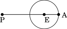
Figure XII.1: Farthest point at time $\tilde{t}$

Figure XII.2: Point reached by left reachable set after some delay

Lemma 79.

Let $\bar{R}_{p}^{k}({\bf p_{0}},t):=R_{p}^{k}({\bf p_{0}},t)/A_{p}(0)$ i.e. the set of points contained in the reachable set of kinematic pursuer except those which belong to the anti-clockwise pursuer circle. For any initial pursuer position ${\bf p_{0}}\in\mathbb{R}^{3}$ and any initial evader position ${\bf e_{0}}\in\mathbb{R}^{3}$the set $\bar{R}_{p}^{k}({\bf p_{0}},t)$ of the kinematic pursuer, starting to move at time $\tilde{t}=(2\pi+2)r_{p}/v_{p_{m}}$, is contained inside the left reachable set of the pursuer having the kinematics of a Dubins vehicle and starting at $t=0$ for all $t\geq\tilde{t}$.

Proof:

Let the pursuer (Dubins vehicle) be located at point P with orientation as shown in Figure XII.2. The dotted circle shown in Figure XII.2 is the left minimum turning radius circle of the pursuer. Also, let $D$ be a point located outside the left pursuer circle as shown in Figure XII.2. The kinematic point is also located at $P$ and stays at point $P$ up to time $\tilde{t}=(2\pi+2)r_{p}/v_{p_{m}}$. Thus, the minimum time required for this kinematic pursuer to reach point $D$, say $t_{1}$, is time it stays at point $P$ ( $t\in[0,\tilde{t}]$) plus time required to cover distance $PD$. Thus, $t_{1}=\tilde{t}+\hat{t}_{1}$, where $\hat{t}_{1}=\text{len}(PD)/v_{p_{m}}$ (since it is constrained to stay at $P$ for time $t\in[0,\tilde{t}]$ ).

Now the minimum time required by $CS$ type of curve given by (III.1) to reach point $D$ is given by

$$t_{2} = \{\text{len(Arc $PAB$)}+\text{len}(BD)\}/v_{p_{m}}$$

Since $\text{len(Arc $PAB$)}\leq 2\pi r_{p}$, $\text{len}(BD)\leq\text{len}(AD)$, and $\text{len}(AD)\leq 2r_{p}+\text{len}(PD)$,

$$t_{2} \leq (2\pi r_{p}+\text{len}(AD))/v_{p_{m}}$$

$$\leq (2\pi r_{p}+2r_{p}+\text{len}(PD))/v_{p_{m}}$$

$$= \hat{t}_{1}+(2\pi+2)r_{p}/v_{p_{m}}=t_{1}$$

Thus $t_{2}\leq t_{1}$ and the claim follows. ∎

Lemma 80.

If $d_{pe}^{0}\geq 2r_{p}+2\pi r_{p}(v_{e_{m}}/v_{p_{m}})$ the pursuer can intercept the evader before it enters anti-clockwise pursuer circle by the trajectories of the type $LS$.

Proof:

Let the pursuer be located at a distance $d_{pe}^{0}$ away from the evader. By the arguments similar to those used in Lemma 49 we can conclude that the evader requires at least time $t_{e}:=[d_{pe}^{0}-2r_{p}]/v_{e_{m}}$ to reach any point on the pursuer’s circle.

Any point on the left pursuer circle can be reached by the pursuer in time $t\leq t_{p}:=2\pi r_{p}/v_{p_{m}}$. Hence if $t_{p}$ is less than the minimum time in which the evader can reach any point on the pursuer circles then the pursuer can intercept the evader before it can enter the anti-clockwise pursuer circle. Thus, if

$$t_{e} \geq t_{p}$$

$${}[d_{pe}^{0}-2r_{p}]/v_{e_{m}} \geq 2\pi r_{p}/v_{p_{m}}$$

$$d_{pe}^{0} \geq 2r_{p}+2\pi r_{p}(v_{e_{m}}/v_{p_{m}})$$

the claim follows. ∎

Proof of Lemma 17

By Lemma 80, even if the evader’s reachable set can extend into the anti-clockwise pursuer circle this part of evader’s reachable set cannot form a part of $R_{e}^{-}({\bf e_{0}},R_{p}^{l},T_{l})$ if $d_{pe}^{0}\geq 2r_{p}+2\pi r_{p}(v_{e_{m}}/v_{p_{m}})$. Similarly, from Lemma 79 we have that the set $\bar{R}_{p}^{k}({\bf p_{0}},t)$ of kinematic pursuer is contained contained inside the reachable set of pursuer. Further, at time $\bar{t}$ the kinematic pursuer’s reachable set contains the reachable set of the kinematic evader (by Lemma 78) and hence the reachable set of the evader (by Lemma 77). This implies that that the reachable set of the evader is contained inside the left reachable set of the pursuer.

Aditya Chaudhrai received the Bachelors degree in Electrical Engineering from University of Mumbai, India, in 2013 and M.Tech. degree from the Indian Institute of Technology Guwahati, India, in 2015. Currently, he is pursuing the Ph. D. degree in Control and Computing at the Indian Institute of Technology Bombay, Mumbai, India. His research interests include time optimal control, pursuit-evasion games, multi-agent systems and adaptive control.

Debraj Chakraborty received the B.E.E. degree from Jadavpur University, Kolkata, India, in 2001, the M.Tech. degree from the Indian Institute of Technology Kanpur, India, in 2003, and the Ph. D. degree from the University of Florida, Gainesville, in 2007. He joined the Indian Institute of Technology Bombay, Mumbai, India, in 2007, where he is currently an Associate Professor in the Department of Electrical Engineering. His research interests include optimal control, linear systems, and multi-agent systems.

References

- [1] R. Isaacs, Differential Games. Dover Publications, 1965.
- [2] A. W. Merz, “The game of two identical cars,” Journal of Optimization Theory and Applications, vol. 9, no. 5, pp. 324–343, 1972.
- [3] I. Exarchos and P. Tsiotras, “An asymmetric version of the two car pursuit-evasion game,” in 53rd IEEE Conference on Decision and Control, 2014.
- [4] R. Bera, V. R. Makkapati, and M. Kothari, “A comprehensive differential game theoretic solution to a game of two cars,” Journal of Optimization Theory and Applications, vol. 174, no. 3, pp. 818–836, Sep 2017.
- [5] I. Exarchos, P. Tsiotras, and M. Pachter, “On the suicidal pedestrian differential game,” Dynamic Games and Applications, vol. 5, no. 3, pp. 297–317, 2015.
- [6] U. Ruiz and R. Murrieta-Cid, “A differential pursuit/evasion game of capture between an omnidirectional agent and a differential drive robot, and their winning roles,” International Journal of Control, vol. 89, no. 11, pp. 2169–2184, 2016.
- [7] U. Ruiz, R. Murrieta-Cid, and J. L. Marroquin, “Time-optimal motion strategies for capturing an omnidirectional evader using a differential drive robot,” IEEE Transactions on Robotics, vol. 29, no. 5, pp. 1180–1196, 2013.
- [8] E. Cockayne, “Plane pursuit with curvature constraints,” SIAM Journal on Applied Mathematics, vol. 15, no. 6, pp. 1511–1516, 1967.
- [9] K. Mizukami and K. Eguchi, “A geometrical approach to problems of pursuit-evasion games,” Journal of the Franklin Institute, vol. 303, no. 4, pp. 371–384, 1977.
- [10] E. Cockayne and G. Hall, “Plane motion of a particle subject to curvature constraints,” SIAM Journal on Control, vol. 13, no. 1, pp. 197–220, 1975.
- [11] X.-N. Bui and J.-D. Boissonnat, “Accessibility region for a car that only moves forwards along optimal paths,” Ph.D. dissertation, INRIA, 1994.
- [12] L. E. Dubins, “On curves of minimal length with a constraint on average curvature, and with prescribed initial and terminal positions and tangents,” American Journal of mathematics, vol. 79, no. 3, pp. 497–516, 1957.
- [13] H. J. Sussmann and G. Tang, “Shortest paths for the reeds-shepp car: a worked out example of the use of geometric techniques in nonlinear optimal control,” Rutgers Center for Systems and Control Technical Report, vol. 10, pp. 1–71, 1991.
- [14] J.-D. Boissonnat, A. Cérézo, and J. Leblond, “Shortest paths of bounded curvature in the plane,” Journal of Intelligent and Robotic Systems, vol. 11, no. 1-2, pp. 5–20, 1994.
- [15] P. Soueres and J.-P. Laumond, “Shortest paths synthesis for a car-like robot,” IEEE Transactions on Automatic Control, vol. 41, no. 5, pp. 672–688, 1996.
- [16] P. Soueres, A. Balluchi, and A. Bicchi, “Optimal feedback control for route tracking with a bounded-curvature vehicle,” International Journal of Control, vol. 74, no. 10, pp. 1009–1019, 2001.
- [17] W. Sun and P. Tsiotras, “Pursuit evasion game of two players under an external flow field,” in American Control Conference, 2015.
- [18] W. Sun, P. Tsiotras, T. Lolla, D. N. Subramani, and P. F. J. Lermusiaux, “Pursuit-evasion games in dynamic flow fields via reachability set analysis,” in American Control Conference, 2017.
- [19] A. W. Merz and D. S. Hague, “Coplanar tail-chase aerial combat as a differential game,” AIAA Journal, vol. 15, no. 10, pp. 1419–1423, 1977.
- [20] F. Imado and T. Ishihara, “Pursuit-evasion geometry analysis between two missiles and an aircraft,” Computers and Mathematics with Applications, vol. 26, no. 6, pp. 125 – 139, 1993.
- [21] J. S. Jang and C. J. Tomlin, “Control strategies in multi-player pursuit and evasion game,” AIAA Guidance, Navigation, and Control Conference and Exhibit, vol. 6239, pp. 15–18, 2005.
- [22] T. Başar and G. J. Olsder, Dynamic noncooperative game theory. SIAM, 1998.
- [23] A. E. Bryson, Applied optimal control: optimization, estimation and control. CRC Press, 1975.
- [24] T. Raivio and H. Ehtamo, On the Numerical Solution of a Class of Pursuit-Evasion Games. Birkhäuser Boston, 2000, pp. 177–192.
- [25] A. Chaudhari, R. Chourasia, and D. Chakraborty, “A computationally efficient feedback solution for a particular case of the game of two cars,” in European Control Conference, 2019.
- [26] J. Betts, Practical Methods for Optimal Control and Estimation Using Nonlinear Programming, 2nd ed. Society for Industrial and Applied Mathematics, 2010.
- [27] A. Wachter and L. T. Biegler, “On the implementation of an interior-point filter line-search algorithm for large-scale nonlinear programming,” Mathematical Programming, vol. 106, no. 1, pp. 25–57, Mar 2006.
- [28] X. Bui, J. Boissonnat, J. Laumond, and P. Soures, “The shortest path synthesis for non-holonomic robots moving forwards, inria, nice-sophia-antipolis,” Research Report 2153, Tech. Rep., 1994.