Variational Bayesian Methods for Stochastically Constrained System Design Problems

Abstract

We study system design problems stated as parameterized stochastic programs with a chance-constraint set. We adopt a Bayesian approach that requires the computation of a posterior predictive integral which is usually intractable. In addition, for the problem to be a well-defined convex program, we must retain the convexity of the feasible set. Consequently, we propose a variational Bayes-based method to approximately compute the posterior predictive integral that ensures tractability and retains the convexity of the feasible set. Under certain regularity conditions, we also show that the solution set obtained using variational Bayes converges to the true solution set as the number of observations tends to infinity. We also provide bounds on the probability of qualifying a true infeasible point (with respect to the true constraints) as feasible under the VB approximation for a given number of samples.

1 Introduction

A general system design problem can be formally stated as the following constraint optimization problem

minimize $$\quad f(x,\xi)$$ (TP)

s.t. $$\quad g_{i}(x,\xi)\leq 0,\ i\in\{1,2,3,\ldots,m\},$$

where $x\in\mathcal{X}\subseteq\mathbb{R}^{p}$ is the input/control vector in a convex set $\mathcal{X}$ and $\xi\in\Theta\subseteq\mathbb{R}^{q}$ is the system parameter vector. The function $f(x,\xi):\mathcal{X}\times\Theta\mapsto\mathbb{R}$ encodes the cost/risk associated with the given values of parameter and control variable $\xi$ and $x$ respectively. Similarly, the functions $g_{i}(x,\xi):\mathcal{X}\times\Theta\mapsto\mathbb{R}$ define the constraints on $\xi$ and $x$. Under certain regularity conditions on the cost and the constraint functions, and for a given value of the true system parameter $\xi_{0}$, the problem (TP) at $\xi=\xi_{0}$ can be solved to obtain the optimal control vector $x^{*}$. In practice, the true system parameters are unknown and these parameters must be estimated using observed data.

In this paper, we take a Bayesian approach and model the uncertainty over the parameters $\xi$ by computing a posterior distribution $\pi(\xi|\mathbf{X}_{n})$ for a given prior distribution $\pi(\xi)$ and the likelihood $P_{\xi}(\mathbf{X}_{n})$ of observing data $\mathbf{X}_{n}$. We approximate the true problem (TP), using the posterior distribution, with the following joint chance-constrained problem:

minimize $$\quad\mathbb{E}_{\pi(\xi|\mathbf{X}_{n})}[f(x,\xi)]$$ (BJCCP)

s.t. $$\quad\pi\left(g_{i}(x,\xi)\leq 0,\ i\in\{1,2,3,\ldots,m\}|\mathbf{X}_{n}\right)\geq\beta,\forall x\in\mathcal{X},$$

where $\beta\in(0,1)$ is the specified confidence level desired by the decision maker (DM) based on the requirement, usually $\beta>\frac{1}{2}$. We provide a supporting example (see Appendix B) to motivate the chance-constraint formulation as opposed to using expectations, in which case the constraints are only satisfied on an average. The unconstrained version of the above problem has been studied as a special case in Jaiswal et al., (2019).

In practice, computing posterior distributions is challenging and mostly intractable, and is typically approximated using Markov Chain Monte Carlo (MCMC) or Variational Bayesian(VB) methods. MCMC methods has its own drawbacks like poor mixing, large variance, and complex diagnostics, which have been the usual motivation for using VB (Blei et al.,, 2017). Here, we provide another important motivation for using VB in the chance-constrained Bayesian inference setting. In particular, we present an example (motivated from Pena-Ordieres et al., (2019)) where a sampling based approach to approximate the chance-constraint convex feasibility set (constraint set) in (BJCCP), results in a non-convex approximation; whereas an appropriate VB approximation retains its convexity. Therefore, we approximate (BJCCP) using a VB approximate posterior $q^{*}(\mathbb{\xi}|\mathbf{X}_{n})$ to $\pi(\xi|\mathbf{X}_{n})$ as:

minimize $$\quad\mathbb{E}_{q^{*}(\mathbb{\xi}|\mathbf{X}_{n})}[f(x,\xi)]$$ (VBJCCP)

s.t. $$\quad q^{*}\left(g_{i}(x,\xi)\leq 0,\ i\in\{1,2,3,\ldots,m\}|\mathbf{X}_{n}\right)\geq\beta,\forall x\in\mathcal{X}.$$

Under certain regularity conditions, we also show that the optimizers of (VBJCCP) are consistent with those of (TP). More precisely, we show that the solution set obtained in (VBJCCP) converges to the true solution set as the number of observations, $n$ tends to infinity. We also provide bounds on the probability of qualifying a true infeasible point (with respect to the true constraints) as feasible under the VB approximation for a given number of samples. As part of the future work, we want to analyze the risk-sensitive VB approximation of the (BJCCP), where the risk is quantified as the deviation of the approximate feasibility set from the true.

2 Variational Bayes for Chance-Constrained System Design

Bayesian statistics delineates natural principles to model uncertainty in parameter estimation, using observed data combined with prior knowledge. Let $\mathbf{X}_{n}=\{X_{1},X_{2},\ldots,X_{n}\}$, be $n$ independent and identically distributed samples from the $\mathcal{F}$ measurable random vector ${X(\omega)}$ with support $\Omega\subset\mathbb{R}^{d}$ on probability space $(\Omega,\mathcal{F},{P_{\xi}})$, with $P_{\xi}$ as the associated probability measure, with parameter $\xi$.

Using the posterior distribution $\pi(\xi|\mathbf{X}_{n})$, we approximate (TP) as a data-driven joint chance-constrained problem, stated formally as:

minimize $$\quad\mathbb{E}_{\pi(\xi|\mathbf{X}_{n})}[f(x,\xi)]$$ (BJCCP)

s.t. $$\quad\pi\left(g_{i}(x,\xi)\leq 0,\ i\in\{1,2,3,\ldots,m\}|\mathbf{X}_{n}\right)\geq\beta,\forall x\in\mathcal{X}.$$

and $\beta\in(0,1)$ is the specified confidence level desired by the decision maker (DM) based on the requirement. These are the two significant challenges in solving (BJCCP):

1. Computing the posterior distribution: While in some cases conjugate priors can be used, this is not acceptable in most problems; resulting in an intractable computation. The posterior intractability is the common motivation for using VB (Blei et al.,, 2017) and MCMC techniques for approximate Bayesian inference.

2. Convexity of the feasibility set: Ideally, one should expect (BJCCP) to be a convex program to take advantage of the well established convex solvers. But, even if the posterior distribution is computable, to qualify (BJCCP) as a convex program, the feasibility set,

   $$\{x\in\mathcal{X}:\pi\left(g_{i}(x,\xi)\leq 0,\ i\in\{1,2,3,\ldots,m\}|\mathbf{X}_{n}\right)\geq\beta\}$$ (1)

   must be convex. It might be possible that the above set is not convex even when the underlying constraint functions $g_{i}(x,\xi),i\in\{1,2,\ldots m\}$ are so (in $x$) and thus finding a global optimum becomes challenging (Prékopa,, 1995).

Note that, if the constraint function has some specified structural regularity and the posterior distribution belongs to a certain class of distributions, then it can be shown that the feasibility set in (1) is convex. For instance, it can be shown that if the constraint functions $g_{i}(x,\xi),i\in\{1,2,\ldots m\}$ are quasi-convex in $(x,\vec{\xi})$ and the distribution is log-concave then the feasibility set in (BJCCP) is convex ((Shapiro et al.,, 2009, Chapter 4) and Prékopa, (2003)). Also, Lagoa et al., (2005) showed that if the constraint function $g_{i}(x,\xi)$ is of the form $\{\vec{a}^{T}x\leq\vec{b}\}$, where $\xi=(\vec{a}^{T},\vec{b})^{T}$ and has a symmetric log-concave density then with $\beta>\frac{1}{2}$ the feasibility set in (BJCCP) is convex.

To address the posterior intractability, Monte Carlo (MC) methods offer one way to do approximate Bayesian inference with asymptotic guarantees. However, their asymptotic guarantees are offset by issues like poor mixing, large variance and complex diagnostics in practical settings with finite computational budgets. Apart from these common issues, there is another important reason due to which any sampling-based method can not be used directly to solve (BJCCP). Using the empirical approximation to the posterior distribution (constructed using the samples generated from MCMC algorithm) to approximate the chance-constraint feasibility set in (BJCCP), results in a non-convex feasibility set (Pena-Ordieres et al.,, 2019). To illustrate this, consider the following simple example (modified slightly) of a chance-constraint feasibility set from Pena-Ordieres et al., (2019). We plot in Figure 1(a) the following chance-constraint feasibility set

$$\left\{x\in R^{2}:\mathcal{N}\left(\vec{\xi}^{T}x-1\leq 0|\mathbb{\mu}=[0,0]^{T},\Sigma_{A}=[1,-0.1;-0.1,1]\right)>\beta\right\},$$ (2)

and its empirical approximator using 8000 MCMC (Metropolis-Hastings with 3000 burn-in samples ) samples generated from the underlying correlated multivariate Gaussian distribution. We observe that the resulting MC approximate feasibility set is non-convex.

Therefore, due to the posterior intractability and the non-convexity of the feasible region when using sampling approaches, as an alternative, we propose to use Variational Bayes (VB) methods.

The idea behind VB is to approximate the intractable posterior $\pi(\xi|\mathbf{X}_{n})$ with an element $q^{*}(\mathbb{\xi}|\mathbf{X}_{n})$ of a simpler variational family $\mathcal{Q}$. Examples of $\mathcal{Q}$ include the family of Gaussian distributions, delta functions, or the family of factorized ‘mean-field’ distributions that discard correlations between components of $\xi$. The variational solution $q^{*}$ is the element of $\mathcal{Q}$ that is ‘closest’ to $\pi(\xi|\mathbf{X}_{n})$, where closeness is usually measured in the Kullback-Leibler (KL) sense. Thus,

$$q^{*}(\mathbb{\xi}|\mathbf{X}_{n}):=\text{argmin}_{{q}\in\mathcal{Q}}\text{KL}({q}(\theta)\|\pi(\xi|\mathbf{X}_{n})).$$ (3)

Using this, we approximate (BJCCP) with,

minimize $$\quad\mathbb{E}_{q^{*}(\mathbb{\xi}|\mathbf{X}_{n})}[f(x,\xi)]$$ (VBJCCP)

s.t. $$\quad q^{*}\left(g_{i}(x,\xi)\leq 0,\ i\in\{1,2,3,\ldots,m\}|\mathbf{X}_{n}\right)\geq\beta,\forall x\in\mathcal{X},$$

where $\beta$ is the confidence level. Choosing the approximation to the posterior distribution from a class of ‘simple’ distributions would facilitate in addressing the two critical problems associated with (BJCCP). Besides the tractability of the posterior distribution, for instance, using the results in Prékopa, (2003) and Lagoa et al., (2005) the choice of a log-concave family of distributions as the approximating family could retain the convexity of the feasibility set, if the constraint functions have certain structural regularity.

Next, we show that using the popular mean-field variational family to approximate the correlated multivariate Gaussian distribution in the same example in (2), we obtain a smooth and convex approximation to the (BJCCP) feasibility set. First, we compute mean-field approximation $q_{A}(\xi)$ and $q_{B}(\xi)$ of $\mathcal{N}\left(\xi|\mathbb{\mu}=[0,0]^{T},\Sigma\right)$ for fours different covariance matrices $\Sigma$, with fixed variance $\sigma_{11}=\sigma_{22}=1$ but varying covariance $\sigma_{12}=\{-0.1,-0.025,0.025,0.1\}$. Then, we plot the respective approximate VB chance-constraint feasibility region in Figure 1. We observe that VB approximation provides a smooth convex approximation to the true feasibility set, but it could be outside the true feasibility region if the $\xi_{1}$ and $\xi_{2}$ are positively correlated.

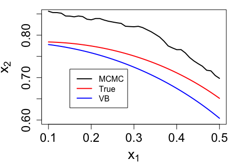
(a) $\sigma^{A}_{12}=-0.1$

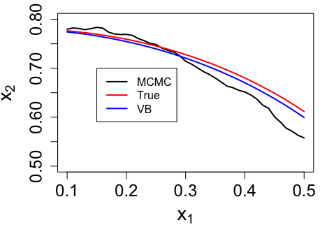
(b) $\sigma^{B}_{12}=-0.025$

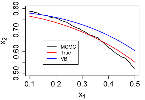
(c) $\sigma^{C}_{12}=0.025$

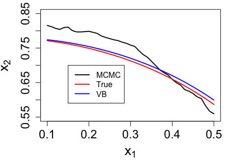
(d) $\sigma^{D}_{12}=0.1$

Figure 1: Feasible Region : True Distribution vs Monte Carlo Approximation (5000 samples) vs. VB (mean field approximation).

2.1 Theoretical properties of (VBJCCP)

In this section, we establish theoretical guarantees on the approximate optimal solution set $\mathcal{S}^{*}_{VB}(\mathbf{X}_{n})$ obtained using the VB approximation and show that it converges to the optimal solution set $\mathcal{S}^{*}$ of (TP) almost surely in $P_{0}$. We show similar result for their corresponding optimal values $V^{*}_{VB}(\mathbf{X}_{n})$ and $V^{*}$. The consistency of the approximate solution follows using techniques from the variational calculus and the consistency of the VB-approximate posterior distribution, which is proved under certain conditions on the prior distribution, likelihood model, and the variational approximation in Wang and Blei, (2018). For brevity, we state the following results without any assumptions and proofs; it will be stated formally in Appendix C.

Proposition 2.1.

We show that $V^{*}_{VB}(\mathbf{X}_{n})\to V^{*}\leavevmode\nobreak\ P_{0}-a.s.$ and $\mathbb{D}(\mathcal{S}^{*}_{VB}(\mathbf{X}_{n}),\mathcal{S}^{*})\to 0\leavevmode\nobreak\ P_{0}-a.s.\leavevmode\nobreak\ \text{as}\leavevmode\nobreak\ n\to\infty$, where $\mathbb{D}(A,B):=\sup_{x\in A}\inf_{\vec{y}\in B}\|x-\vec{y}\|,$ is the distance between two sets $A$ and $B$.

In the next result, we show that the solution obtained in (VBJCCP) are feasible with high probability. Let us define the set where the true constraint $i\in\{1,2,\ldots m\}$ is satisfied as $F^{i}_{0}:=\{x\in\mathcal{X}:\{g_{i}(x,\xi_{0})\leq 0\},\},$ and VB-approximate feasibility set is denoted as $\hat{F}_{VB}(\mathbf{X}_{n}):=\{x\in\mathcal{X}:q^{*}\left(g_{i}(x,\xi)\leq 0,\ i\in\{1,2,3,\ldots,m\}|\mathbf{X}_{n}\right)\geq\beta\}.$ We prove the next result using the convergence rate results for VB approximation in Zhang and Gao, (2019).

Proposition 2.2.

We show that if $x\in\mathcal{X}\backslash F_{0}^{i}$, then there exists constant $C_{i}>0$ for each $i\in\{1,2,\ldots m\}$, such that $\mathbb{P}_{0}[x\in\hat{F}_{VB}(\mathbf{X}_{n})]\leq\frac{C_{i}}{\beta}(\epsilon_{n}^{2}+\eta_{n}^{2}),$ where $\epsilon_{n}^{2}\to 0$ as $n\to\infty$ and $\eta_{n}^{2}:=\frac{1}{n}\inf_{q\in\mathcal{Q}}\mathbb{E}_{P_{0}}\left[\int_{\Theta}q(\xi)\log\frac{q(\xi)}{\pi(\xi|\mathbf{X}_{n})}d\xi d\xi\right].$

Appendix A A System Design Problem

To illustrate the system design problem in (TP) with an example, we model a queueing system and show that the optimal staffing problem aptly fits into the above framework. Consider a staffing problem where the decision maker (DM) has to decide the optimal number of servers, $c$, after observing the arrival and service data in an $M/M/c$ queueing system; a queueing system where the inter-arrival times and service times are exponentially distributed (Markovian) with $c$ number of servers, is denoted as $M/M/c$ queueing system. We assume that the rate parameters of the exponentially distributed inter-arrival and service times distribution are unknown and denoted as $\lambda$ and $\mu$ respectively. Note that $\lambda$ and $\mu$, combined together form the system parameter $\xi=\{\lambda,\mu\}$ and the number of servers $c$ is the control/input variable. The DM first uses a single server and collects data after the system reaches its ‘steady state’. Since the DM observed congestion in the queues, he/she decides to employ more servers. The DM collects $n$ realizations of the random vector $\mathcal{V}:=\{T,S,E\}$, denoted as $\mathbf{X}_{n}:=\{\mathcal{V}_{1},\ldots\mathcal{V}_{n}\}$ where $T$, $S$, and $E$ are the random variables denoting the arrival, service-start, and service-end time of each customer $i\in\{1,2,\ldots n\}$ respectively. We also assume that there is no time lag between the two successive states for any customer and the inter-arrival and service times are independent, that is $T_{i}-T_{i-1}$ is independent of $E_{i}-S_{i}$ for each $i\geq 1$. The joint likelihood of the arrival and departure times for $n$ customers is

$$P_{\xi}(\mathbf{X}_{n}):=\prod_{i=1}^{n}\lambda e^{-\lambda(T_{i}-T_{i-1})}\mu e^{-\mu(E_{i}-S_{i})}.$$

Constraint functions: The DM chooses the number of servers $c$ to maintain a constant measure of congestion. Congestion is usually measured as $1-W_{q}(c,\lambda,\mu)$, where $W_{q}(c,\lambda,\mu)$ is the probability that the customer did not wait in the queue. The closed-form expression for $1-W_{q}(c,\lambda,\mu)$ is known to be (see Gross et al., (2008))

$$1-W_{q}(c,\lambda,\mu)=\frac{r^{c}}{c!(1-\rho)}\Bigg{/}\left(\frac{r^{c}}{c!(1-\rho)}+\sum_{t=0}^{c-1}\frac{r^{t}}{t!}\right),$$

where $r=\frac{\lambda}{\mu}\text{ and }\rho=\frac{r}{c}$ with $\rho<1$. $\rho$ is also known as traffic intensity and for a stable queue $\rho<1$. DM fixes $\alpha$, which is maximum desired fraction of customers delayed in queue and the smallest $c$ is chosen that satisfies:

$$(\alpha-\{1-W_{q}(c,\lambda,\mu)\})>0\text{ and }(c\mu-\lambda)>0.$$

Referring to the queueing literature, we will use the term the Quality of Service(QoS) constraint for the first constraint. The corresponding constraint optimization problem is

minimize $$\quad c$$ (TP-Q)

s.t. $$\quad(\alpha-\{1-W_{q}(c,\xi)\})>0\quad\textsc{(QoS)},$$

$$\quad(c\mu-\lambda)>0.$$

The above staffing problem and its variations are well studied in the queueing literature; interested reader may refer to Gans et al., (2003) and Aksin et al., (2009).

Appendix B Other Data-Driven Approaches to solve (TP)

Since the system parameters are unknown in practice, these are usually estimated using the observed data $\mathbf{X}_{n}$. The simplest approach could be to substitute the maximum likelihood estimates(MLE) $\hat{\xi}(\mathbf{X}_{n})$ of the parameters $\xi$ in the (TP) and solve the following approximate problem:

minimize $$\quad f(x,\hat{\xi})$$ (TP-MLE)

s.t. $$\quad g_{i}(x,\hat{\xi})\leq 0,\ i\in\{1,2,3,\ldots,m\}.$$

We solved the queueing staffing problem in Appendix A using the MLE approach on simulated data ($n$ observations, with $n$ in 50-400 in increments of 50) and computed the approximate optimal number of servers denoted as $C^{n}_{MLE}$. We repeated this experiment over 100 sample paths and computed $\phi(C^{n}_{MLE})$, the fraction of experiments $C^{n}_{MLE}$ violates the QoS constraint. Table 1 shows that the QoS constraint is violated in over 50% of the experiments.

$n$	50	100	150	200	250	300	350	400
$\phi(C^{n}_{MLE})$	0.52	0.56	0.57	0.57	0.61	0.62	0.58	0.56

Table 1: Fraction of times $C^{n}_{MLE}$ violates QoS constraint. $\lambda_{0}=16,\mu_{0}=4,\alpha=0.37$.

It is anticipated that the MLE approach is unable to capture the uncertainty in parameter estimation therefore an alternative method is proposed using forecasting techniques. In this approach first, the uncertainty over the parameter estimation is captured by forecasting a probability distribution $P(\xi)$ over the system parameters and then the forecast distribution is used to solve the (TP) problem using one of the following two formulations:

• Average-Constraint(AC)

  minimize $$\quad\mathbb{E}_{P}[f(x,\xi)]$$ (TP-FAC)

  s.t. $$\quad\mathbb{E}_{P}[g_{i}(x,\xi)]\leq 0,\ i\in\{1,2,3,\ldots,m\},$$

• Chance-Constraint(CC)

  minimize $$\quad\mathbb{E}_{P}[f(x,\xi)]$$ (TP-FCC)

  s.t. $$\quad P\left\{g_{i}(x,\xi)\leq 0,\ i\in\{1,2,3,\ldots,m\}\right\}>\beta,$$

  where $\beta\in(0,1)$ is the confidence level.

Now consider a simple example from Hong et al., (2011), where the true problem is to find $c^{*}=\min\{c:\xi-c\leq 0\}$. Since, $\xi$ is unknown the DM uses data to forecast that $\xi\sim\mathcal{N}(\cdot|0,1)$ is normally distributed. Using the AC formulation, notice that the approximate optimal solution $c_{A}^{*}=\min\{c:\mathbb{E}_{\xi}[\xi]-c\leq 0\}=0$ and $\mathbb{P}_{\xi}\{\xi\geq c_{A}^{*}\}=0.5$. The above simple example shows that AC optimal solution could violate the constraint 50% of the times. On the other hand, CC formulation enables the DM to ensure that the approximate optimal solution satisfy the constraints with higher confidence by setting a higher confidence level($\beta$). In forecasting approach, the DM needs to forecast each time the new data is collected. We propose a principled data-driven approach using Bayesian methods, wherein we combine forecasting and optimization. A similar approach has also been discussed in Aktekin and Ekin, (2016) to solve the $M/M/c$ staffing problem with abandonment, but crucially relies on the availability of conjugate priors.

Appendix C Proofs

C.1 Proof of Proposition 2.1

Assumption C.1.

We assume that the function $f(x,\xi)$ and $g_{i}(x,\xi),\forall i\in\{1,2,\ldots m\}$ are Carathéodory functions; that is $f(x,\cdot)$ and $g_{i}(x,\cdot)$ are measurable for every $x\in\mathcal{X}$, and $f(\cdot,\xi)$ and $g(\cdot,\xi)$ are continuous for almost every $\xi\in\Theta$. We also assume that $f(\cdot,\xi)$ is locally Lipschitz continuous in $x$ for almost every $\xi\in\Theta$ and $f(x,\cdot)$ is uniformly integrable with respect to any $q\in\mathcal{Q}$, the variational family.

Next define an indicator function $\mathbb{I}_{(-\infty,0]}(t):=1\text{ if $t\leq 0$ and }0\text{ if $t>0$ }$.

Lemma C.1.

We show that for each $x\in\mathcal{X}$

$$\lim_{n\to\infty}q^{*}\left(\prod_{i=1}^{m}\mathbb{I}_{(-\infty,0]}(g_{i}(x,\xi))|\mathbf{X}_{n}\right)=\prod_{i=1}^{m}\mathbb{I}_{(-\infty,0]}(g_{i}(x,\xi_{0}))\leavevmode\nobreak\ P_{0}-a.s.$$

Proof.

Recall the result in Wang and Blei, (2018) that the VB approximate posterior $q^{*}(\mathbb{\xi}|\mathbf{X}_{n})$ is consistent; that is for every $\eta>0$.

$$\lim_{n\to\infty}\int_{\|\xi-\xi_{0}\|>\eta}q^{*}(\mathbb{\xi}|\mathbf{X}_{n})d\xi=0\leavevmode\nobreak\ P_{0}-a.s.$$ (4)

Observe that for any $x\in\mathcal{X}$ and $\eta>0$,

$$q^{*}\left(\prod_{i=1}^{m}\mathbb{I}_{(-\infty,0]}(g_{i}(x,\xi))|\mathbf{X}_{n}\right) =\int_{\Theta}\prod_{i=1}^{m}\mathbb{I}_{(-\infty,0]}(g_{i}(x,\xi))q^{*}(\mathbb{\xi}|\mathbf{X}_{n})d\xi$$

$$=\int_{\|\xi-\xi_{0}\|>\eta}\prod_{i=1}^{m}\mathbb{I}_{(-\infty,0]} (g_{i}(x,\xi))q^{*}(\mathbb{\xi}|\mathbf{X}_{n})d\xi+\int_{\|\xi-\xi_{0}\|\leq\eta}\prod_{i=1}^{m}\mathbb{I}_{(-\infty,0]}(g_{i}(x,\xi))q^{*}(\mathbb{\xi}|\mathbf{X}_{n})d\xi.$$ (5)

Observe that, the result in (4) combined with the fact that the first term in (5) is always positive and bounded, implies that $\lim_{n\to\infty}\int_{\|\xi-\xi_{0}\|>\eta}\prod_{i=1}^{m}\mathbb{I}_{(-\infty,0]}(g_{i}(x,\xi))q^{*}(\mathbb{\xi}|\mathbf{X}_{n})d\xi=0\leavevmode\nobreak\ P_{0}-a.s$. Now taking limits on either side of (5), we have

$$\lim_{n\to\infty}q^{*}\left(\prod_{i=1}^{m}\mathbb{I}_{(-\infty,0]}(g_{i}(x,\xi))|\mathbf{X}_{n}\right) =\lim_{n\to\infty}\int_{\|\xi-\xi_{0}\|\leq\eta}\prod_{i=1}^{m}\mathbb{I}_{(-\infty,0]}(g_{i}(x,\xi))q^{*}(\mathbb{\xi}|\mathbf{X}_{n})d\xi\leavevmode\nobreak\ P_{0}-a.s,$$

$$=\prod_{i=1}^{m}\mathbb{I}_{(-\infty,0]}(g_{i}(x,\xi_{0}))\leavevmode\nobreak\ P_{0}-a.s$$ (6)

and the lemma follows. ∎

Next we define hypo-convergence and epi-convergence of a sequence of function $\{h_{k}(x)\}$ to $h(x)$.

Definition C.1 (Hypo-convergence).

A sequence of functions $\{h_{k}(x)\}$ hypo-converges to $h(x)$; that is $\text{hypo}-\lim_{n\to\infty}h_{k}(x)=h(x)$, if

1. for every $x_{k}\to x$, $\limsup_{k\to\infty}h_{k}(x_{k})\leq h(x)$, and

2. there exists a sequence $x_{k}\to x$, such that $\liminf_{k\to\infty}h_{k}(x_{k})\geq h(x)$.

Definition C.2 (Epi-convergence).

A sequence of functions $\{h_{k}(x)\}$ epi-converges to $h(x)$; that is $\text{ep}-\lim_{n\to\infty}h_{k}(x)=h(x)$, if

1. for every $x_{k}\to x$, $\liminf_{k\to\infty}h_{k}(x_{k})\geq h(x)$, and

2. there exists a sequence $x_{k}\to x$, such that $\limsup_{k\to\infty}h_{k}(x_{k})\leq h(x)$.

Lemma C.2.

Under Assumption C.1, we show that,

1. for each $x\in\mathcal{X}$, $\lim_{n\to\infty}\mathbb{E}_{q^{*}(\mathbb{\xi}|\mathbf{X}_{n})}[f(x,\xi)]=f(x,\xi_{0})\leavevmode\nobreak\ P_{0}-a.s.$

2. and, $\text{ep}-\lim_{n\to\infty}\mathbb{E}_{q^{*}(\mathbb{\xi}|\mathbf{X}_{n})}[f(x_{n},\xi)]=f(x_{0},\xi_{0})\leavevmode\nobreak\ P_{0}-a.s$.

Proof.

Due to Assumption C.1, both the results above are a direct consequence of the result in (Dupacova and Wets,, 1988, Theorem 3.7). ∎

Lemma C.3.

We show that under Assumption C.1, $q^{*}\left(\prod_{i=1}^{m}\mathbb{I}_{(-\infty,0]}(g_{i}(x,\xi))|\mathbf{X}_{n}\right)$ hypo-converges to $\prod_{i=1}^{m}\mathbb{I}_{(-\infty,0]}(g_{i}(x,\xi_{0}))$ $P_{0}-a.s$ as $n\to\infty$; that is

$$\text{hypo}-\lim_{n\to\infty}q^{*}\left(\prod_{i=1}^{m}\mathbb{I}_{(-\infty,0]}(g_{i}(x,\xi))|\mathbf{X}_{n}\right) =\prod_{i=1}^{m}\mathbb{I}_{(-\infty,0]}(g_{i}(x,\xi_{0}))\leavevmode\nobreak\ P_{0}-a.s.$$ (7)

Proof.

Since by Assumption C.1 each $g_{i}(x,\xi_{0})$ is continuous in $x$, therefore $\mathbb{I}_{(-\infty,0]}(g_{i}(x,\xi_{0}))$ is upper-semicontinuous(USC) in $x$ because $\mathbb{I}_{(-\infty,0]}(\cdot)$ is USC. Also, since the product of non-negative USC functions are also USC, it follows that $\prod_{i=1}^{m}\mathbb{I}_{(-\infty,0]}(g_{i}(x,\xi_{0}))$ is USC. Similarly, since by assumption $g_{i}(x,\xi)$ is Carathéodory function, therefore $\prod_{i=1}^{m}\mathbb{I}_{(-\infty,0]}(g_{i}(x,\xi))$ is a random upper-semicontinuous function (Dupacova and Wets,, 1988). Now, using the reverse Fatou’s Lemma, for any $x_{k}\to x_{0}$

$$\limsup_{x_{k}\to x_{0}}\int_{\Theta}\prod_{i=1}^{m}\mathbb{I}_{(-\infty,0]}(g_{i}(x,\xi))q^{*}(\mathbb{\xi}|\mathbf{X}_{n})d\xi \leq\int_{\Theta}\limsup_{x_{k}\to x_{0}}\prod_{i=1}^{m}\mathbb{I}_{(-\infty,0]}(g_{i}(x,\xi))q^{*}(\mathbb{\xi}|\mathbf{X}_{n})d\xi$$

$$\leq\int_{\Theta}\prod_{i=1}^{m}\mathbb{I}_{(-\infty,0]}(g_{i}(x_{0},\xi))q^{*}(\mathbb{\xi}|\mathbf{X}_{n})d\xi,$$ (8)

therefore $\int_{\Theta}\prod_{i=1}^{m}\mathbb{I}_{(-\infty,0]}(g_{i}(x,\xi))q^{*}(\mathbb{\xi}|\mathbf{X}_{n})d\xi$ is also upper-semicontinuous in $x$. Also, since $-\prod_{i=1}^{m}\mathbb{I}_{(-\infty,0]}(g_{i}(x,\xi))\in\{-1,0\}$ is a bounded random lower-semicontinuous function and $q^{*}(\mathbb{\xi}|\mathbf{X}_{n})\Rightarrow\delta_{\xi_{0}}\leavevmode\nobreak\ P_{0}-a.s$ (Wang and Blei,, 2018), Theorem 3.7 in Dupacova and Wets, (1988) implies that

$$\text{hypo}-\lim_{n\to\infty}q^{*}\left(\prod_{i=1}^{m}\mathbb{I}_{(-\infty,0]}(g_{i}(x,\xi))|\mathbf{X}_{n}\right) =\prod_{i=1}^{m}\mathbb{I}_{(-\infty,0]}(g_{i}(x,\xi_{0}))\leavevmode\nobreak\ P_{0}-a.s;$$ (9)

and the result follows. ∎

Proof of Proposition 2.1.

We will first show that the assertion of the theorem is true for $m=1$. Recall $\mathcal{S}^{*}_{VB}(\mathbf{X}_{n})$ is the solution of (VBJCCP): and $\mathcal{S}^{*}$ is the solution of (TP).

Now observe that, since both $q^{*}\left(g(x,\xi)\leq 0|\mathbf{X}_{n}\right)$ and $\mathbb{I}_{(-\infty,0]}(g(x,\xi_{0}))$ are upper- semicontinuous their corresponding super-level sets are closed; and if $\mathcal{X}$ is bounded than the corresponding feasible sets are also compact. Also, if the the corresponding feasibility sets are non-empty then the corresponding optimal sets $\mathcal{S}^{*}_{VB}(\mathbf{X}_{n})$ and $\mathcal{S}^{*}$ are also non-empty.

Next let us assume that there exists a true solution $x^{*}$ of (TP) which lies in the interior of $\mathcal{X}$, that is for any $\epsilon>0$, there is $x\in\mathcal{X}$ such that $\|x-x^{*}\|<\epsilon$ and $g(x,\xi_{0})\leq 0$. It implies that there exists a sequence $\{x_{k}\}\subset\mathcal{X}$ such that $x_{k}\to x^{*}$ as $k\to\infty$ and $g(x_{k},\xi_{0})\leq 0$ for all $k\geq 1$. Now fix $x\in\mathcal{X}$ such that $g(x,\xi_{0})\leq 0$. Since, due to our result in Lemma C.1 $q^{*}\left(g(x,\xi)\leq 0|\mathbf{X}_{n}\right)$ converges pointwise to $\mathbb{I}_{(-\infty,0]}(g(x,\xi_{0}))\leavevmode\nobreak\ P_{0}-a.s$, therefore there exists an $n_{0}$ such that for all $n\geq n_{0}$, we have $q^{*}\left(g(x,\xi)\leq 0|\mathbf{X}_{n}\right)\geq\beta$. Hence for all $n\geq n_{0}$, $x$ is a feasible solution of (VBJCCP) and therefore $\mathbb{E}_{q^{*}(\mathbb{\xi}|\mathbf{X}_{n})}[f(x,\xi)]\geq V_{VB}^{*}(\mathbf{X}_{n})$. Taking $\limsup$ on either sides, we obtain

$$\limsup_{n\to\infty}V_{VB}^{*}(\mathbf{X}_{n})\leq\limsup_{n\to\infty}\mathbb{E}_{q^{*}(\mathbb{\xi}|\mathbf{X}_{n})}[f(x,\xi)]=f(x,\xi_{0})\leavevmode\nobreak\ P_{0}-a.s,$$

where the last inequality follows from Lemma C.2 (1). Now, since $x$ can be chosen arbitrarily close to $x^{*}$, it follows that

$$\limsup_{n\to\infty}V_{VB}^{*}(\mathbf{X}_{n})\leq f(x^{*},\xi_{0})=V^{*}\leavevmode\nobreak\ P_{0}-a.s.$$ (10)

Next, let $\hat{x}_{n}\in\mathcal{S}_{VB}^{*}$; that is $\hat{x}_{n}\in\mathcal{X}$, $q^{*}\left(g(\hat{x}_{n},\xi)\leq 0|\mathbf{X}_{n}\right)\geq\beta$ and $V_{VB}^{*}(\mathbf{X}_{n})=\mathbb{E}_{q^{*}(\mathbb{\xi}|\mathbf{X}_{n})}[f(\hat{x}_{n},\xi)]$. Since $\mathcal{X}$ is compact, we assume that $\hat{x}_{n}\to x^{*}\leavevmode\nobreak\ P_{0}-a.s$. Due to Lemma C.3, $q^{*}\left(g(x,\xi)\leq 0|\mathbf{X}_{n}\right)$ hypo-converges to $\mathbb{I}_{(-\infty,0]}(g(x,\xi_{0}))$ $P_{0}-a.s$ as $n\to\infty$, therefore we have

$$\limsup_{n\to\infty}q^{*}\left(g(\hat{x}_{n},\xi)\leq 0|\mathbf{X}_{n}\right)\leq\mathbb{I}_{(-\infty,0]}(g(x^{*},\xi_{0})).$$ (11)

Now using the fact that $q^{*}\left(g(\hat{x}_{n},\xi)\leq 0|\mathbf{X}_{n}\right)\geq\beta$ for every $n\geq 1$, it follows from (11) that $x^{*}$ is a feasible point of (TP), since $\limsup_{n\to\infty}q^{*}\left(g(\hat{x}_{n},\xi)\leq 0|\mathbf{X}_{n}\right)\geq\beta$ implies $\mathbb{I}_{(-\infty,0]}(g(x^{*},\xi_{0}))\geq\beta$ and $\beta\in(0,1)$. Therefore, it follows that $f(x^{*},\xi_{0})\geq V^{*}$. Since, due to Lemma C.2 (2), $\liminf_{n\to\infty}\mathbb{E}_{q^{*}(\mathbb{\xi}|\mathbf{X}_{n})}[f(\hat{x}_{n},\xi)]\geq f(x^{*},\xi_{0})\leavevmode\nobreak\ P_{0}-a.s$, it follows that

$$\liminf_{n\to\infty}V_{VB}^{*}(\mathbf{X}_{n})\geq V^{*}\leavevmode\nobreak\ P_{0}-a.s.$$ (12)

Hence, it follows from (10) and (12) that $V_{VB}^{*}(\mathbf{X}_{n})\to V^{*}\leavevmode\nobreak\ P_{0}-a.s$ and it also follows that $x^{*}$ is the true solution of (TP), therefore $\mathbb{D}(\mathcal{S}_{VB}^{*}(\mathbf{X}_{n}),\mathcal{S}^{*})\to 0\leavevmode\nobreak\ P_{0}-a.s$. The above arguments can be easily generalized for the general case with $m$ number of constraints. ∎

C.2 Proof of Proposition 2.2

Proof.

Using Markov’s inequality observe that for any $x\in\mathcal{X}$,

$$\mathbb{P}_{0}[q^{*}\left(g_{i}(x,\xi)\leq 0,\ i\in\{1,2,3,\ldots,m\}|\mathbf{X}_{n}\right)\geq\beta] \leq\frac{1}{\beta}\mathbb{E}_{0}[q^{*}\left(\cap_{i=1}^{m}\{g_{i}(x,\xi)\leq 0\}|\mathbf{X}_{n}\right)]$$

$$\leq\frac{1}{\beta} \mathbb{E}_{0}[q^{*}\left(\{g_{i}(x,\xi)\leq 0\}|\mathbf{X}_{n}\right)]\leavevmode\nobreak\ \forall i\in\{1,\ldots,m\}.$$ (13)

Fix $i\in\{1,2\ldots,m\}$. Since $x\in\mathcal{X}\backslash F^{i}_{0}$ implies that $x\in\{g_{i}(x,\xi_{0})>0\}$, it follows that

$$\{g_{i}(x,\xi)\leq 0\}\subseteq\{g_{i}(x,\xi)<g_{i}(x,\xi_{0})\}.$$

Therefore, for all $x\in\mathcal{X}\backslash F^{i}_{0}$ and any $i\in\{1,\ldots,m\}$, it follows from (13) that

$$\mathbb{P}_{0}[q^{*}\left(g_{i}(x,\xi)\leq 0,\ i\in\{1,2,3,\ldots,m\}|\mathbf{X}_{n}\right)\geq\beta] \leq\frac{1}{\beta}\mathbb{E}_{0}[q^{*}\left(\cap_{i=1}^{m}\{g_{i}(x,\xi)\leq 0\}|\mathbf{X}_{n}\right)]$$

$$\leq\frac{1}{\beta}\mathbb{E}_{0}[q^{*}\left(\{g_{i}(x,\xi)<g_{i}(x,\xi_{0})\}|\mathbf{X}_{n}\right)].$$ (14)

Now using Theorem 2.1 in Zhang and Gao, (2019), it follows that for each $i\in\{1,2,3,\ldots,m\}$ if

$$L^{i}_{n}(\theta,\theta_{0}):=n\sup_{x\in\mathcal{X}}\mathbb{I}_{(0,\infty)}(g_{i}(x,\xi_{0})-g_{i}(x,\xi))$$

satisfies assumption (C1), then there exists a constant $C_{i}$ for each $i\in\{1,2,3,\ldots,m\}$ such that

$$\mathbb{E}_{0}[q^{*}\left(\{g_{i}(x,\xi)<g_{i}(x,\xi_{0})\}|\mathbf{X}_{n}\right)]\leq C_{i}(\epsilon_{n}^{2}+\eta_{n}^{2}),$$

where $\eta_{n}^{2}:=\frac{1}{n}\inf_{q\in\mathcal{Q}}\mathbb{E}_{P_{0}}\left[\int_{\Theta}q(\xi)\log\frac{q(\xi)}{\pi(\xi|\mathbf{X}_{n})}d\xi d\xi\right]$. Now observe that, using the above result in (14) directly proves the assertion of the proposition. ∎

References

• Aksin et al., (2009) Aksin, Z., Armony, M., and Mehrotra, V. (2009). The modern call center: A multi-disciplinary perspective on operations management research. Production and Operations Management, 16(6):665–688.
• Aktekin and Ekin, (2016) Aktekin, T. and Ekin, T. (2016). Stochastic call center staffing with uncertain arrival, service and abandonment rates: A bayesian perspective. Naval Research Logistics (NRL), 63(6):460–478.
• Blei et al., (2017) Blei, D. M., Kucukelbir, A., and McAuliffe, J. D. (2017). Variational inference: A review for statisticians. Journal of the American Statistical Association.
• Dupacova and Wets, (1988) Dupacova, J. and Wets, R. (1988). Asymptotic behavior of statistical estimators and of optimal solutions of stochastic optimization problems. The Annals of Statistics, 16(4):1517–1549.
• Gans et al., (2003) Gans, N., Koole, G., and Mandelbaum, A. (2003). Telephone call centers: Tutorial, review, and research prospects. Manufacturing & Service Operations Management, 5(2):79–141.
• Gross et al., (2008) Gross, D., Shortie, J. F., Thompson, J. M., and Harris, C. M. (2008). Simple Markovian Queueing Models. Wiley.
• Hong et al., (2011) Hong, L. J., Yang, Y., and Zhang, L. (2011). Sequential convex approximations to joint chance constrained programs: A monte carlo approach. Operations Research, 59(3):617–630.
• Jaiswal et al., (2019) Jaiswal, P., Honnappa, H., and Rao, V. A. (2019). Risk-sensitive variational bayes: Formulations and bounds. arXiv preprint arXiv:1903.05220v3.
• Lagoa et al., (2005) Lagoa, C. M., Li, X., and Sznaier, M. (2005). Probabilistically constrained linear programs and risk-adjusted controller design. SIAM Journal on Optimization, 15(3):938–951.
• Pena-Ordieres et al., (2019) Pena-Ordieres, A., Luedtke, J. R., and Wachter, A. (2019). Solving chance-constrained problems via a smooth sample-based nonlinear approximation.
• Prékopa, (1995) Prékopa, A. (1995). Stochastic Programming. Springer Netherlands.
• Prékopa, (2003) Prékopa, A. (2003). Probabilistic programming. Handbooks in operations research and management science, 10:267–351.
• Shapiro et al., (2009) Shapiro, A., Dentcheva, D., and Ruszczyński, A. (2009). Lectures on stochastic programming: modeling and theory. SIAM.
• Wang and Blei, (2018) Wang, Y. and Blei, D. M. (2018). Frequentist consistency of variational bayes. Journal of the American Statistical Association, 0(0):1–15.
• Zhang and Gao, (2019) Zhang, F. and Gao, C. (2019). Convergence rates of variational posterior distributions. Annals of Statistics.