Simulation of topological phases with color center arrays in phononic crystals

Abstract

We propose an efficient scheme for simulating the topological phases of matter based on silicon-vacancy (SiV) center arrays in phononic crystals. This phononic band gap structure allows for long-range spin-spin interactions with a tunable profile. Under a particular periodic microwave driving, the band-gap mediated spin-spin interaction can be further designed with the form of the Su-Schrieffer-Heeger (SSH) Hamiltonian. In momentum space, we investigate the topological characters of the SSH model, and show that the topological nontrivial phase can be obtained through modulating the periodic driving fields. Furthermore, we explore the zero-energy topological edge states at the boundary of the color center arrays, and study the robust quantum information transfer via the topological edge states. This setup provides a scalable and promising platform for studying topological quantum physics and quantum information processing with color centers and phononic crystals.

I introduction

Topological phases of matter have attracted great interests and developed potential applications in quantum physics nat-496-196 (1, 2, 3, 4, 5, 6, 7, 8, 9). In particular, topological insulators possess topologically protected surface or edge states, robust to local disorders. The Su-Schrieffer-Heeger (SSH) model, originally derived from the dimerized chain, is the simplest example of a one-dimensional (1D) topological insulator prl-42-1698 (10, 11). For the generalized SSH Hamiltonian, the interaction between different sites of a 1D chain is described by the alternating off-diagonal elements. Due to the intrinsic topological features of the SSH model, various quantum systems are employed to simulate the SSH model, and to explore interesting applications in quantum information processing prb-89-085111 (12, 13, 14, 15, 16, 17, 18, 19, 20, 21, 22, 23, 24). However, the simulation of topological phenomena in the quantum domain is still challenging in practice due to stringent conditions.

The fundamental model of quantum optics is the light-matter interaction at the single photon level book-1997 (25). Photons play a key role in quantum information science due to their excellent coherence and controllability. With the advent of quantum acoustics, phonons provide an alternative way to store and transmit quantum information in hybrid quantum devices nsr-2-510 (26). Moreover, the low speed of phonons enables new dynamic control protocols for quantum information, and the relatively long acoustic wavelength allows regimes of atomic physics to be explored that cannot be reached in photonic systems. In general, there are two types of phonons in quantum systems. One is in the form of the stationary phonon. In this case, the vibrational eigenmode of mechanical resonators is taken as the phonon mode SCI-335-1603 (27, 28, 29, 30, 31, 32, 33). The other is the propagating phonon, which is resulting from the mechanical lattice vibration in various acoustic setups, such as surface acoustic wave (SAW) devices prb-54-13878 (34, 35, 36, 37, 38), and phononic crystal structures sci-271-634 (39, 40, 41, 42, 43, 44, 45, 46).

Recently, much attention has been paid to the coherent coupling between the phononic structures and other quantum systems prb-79-041302(R) (47, 48, 49, 50, 51, 52, 53, 54, 55). We have investigated the coherent coupling between silicon-vacancy (SiV) centers and the quantized acoustic modes in a one-dimensional phononic crystal waveguide arxiv-2019 (56). Color centers in diamond, owing to their long coherence time and excellent optical properties, have become one of the most promising solid-state quantum emitters np-7-879 (57, 58, 59, 60, 61, 62, 63, 64). The coupling between solid-state spins and quantized acoustic modes in phononic crystals offers new paradigm for investigating spin-phonon interactions near the phonon band-gap. In analogy to photonic crystals, phononic crystals are constructed with elastic waves propagating in periodic structures modulated by periodic elastic modula and mass densities. For phononic crystals, one of the most prominent features is the presence of band-gap structures, which provide stronger interactions due to the much tighter confinement of the mediating phonon prb-49-2313 (65, 66). More importantly, phononic crystals offer a promising platform for practical quantum technologies because of the extremely low thermoelastic mechanical dissipation.

In this work, we present a periodic driving protocol to simulate topological phases with a color center-phononic crystal system in both the one-dimensional (1D) and 2D cases. In the setup, SiV center arrays are coupled to the quantized modes of a phononic crystal near the band-gap. With the band gap engineered spin-phonon interaction, the phononic crystal modes are distributed around the spins with an exponentially decaying envelope. We show that the SSH-type Hamiltonian can be obtained by applying periodic microwave driving fields to the SiV spins. Then we explore the topological properties of the effective spin-spin system in the momentum space. Furthermore, we also study the zero-energy topological edge states at the boundary of the color center array, and show the robust quantum information transfer via the topological edge states. Compared with other nanomechanical systems, phononic crystals possess unique band gap structures and exceptional physical properties, providing an ideal interface with diamond defect spins. Moreover, suitably designed periodic driving fields enable the highly controllable and tunable SSH model in SiV center arrays. Our results allow to further explore the topological properties of the spin-phonon systems, and also open up new ways for quantum information processing in phononic crystal systems.

II Simulation of the 1D SSH model

II.1 The setup

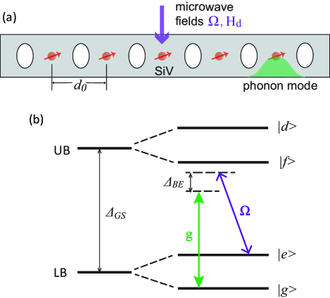
Figure 1: (Color online) (a) Schematics of the hybrid device studied in this work. An array of SiV centers are implanted evenly in a 1D phononic crystal waveguide. $d_{0}$ is the distance between the adjacent spins. The spins are driven by microwave field $\Omega$ and the periodic driving fields $\hat{H}_{d}$. (b) Simplified energy levels of a single SiV center in the electronic ground state. Here, $g$ describes the spin-phonon interaction, $\Delta_{BE}$ is the detuning between the effective spin transition and the phononic band edge frequency.

We first consider a spin-phononic crystal system as shown in Fig. $1(a)$, an array of $2N$ SiV centers are implanted evenly in a 1D phononic crystal waveguide. The generalization of this 1D scheme to the case of 2D will be considered later. The diamond waveguide is perforated with periodic elliptical air holes, which provide the tunable phononic band structure. In general, the phononic crystal supports acoustic guide modes $\omega_{n,k}$, where $n$ is the band index and $k$ is the wave vector along the waveguide direction. The mechanical displacement mode profile $\vec{Q}(\vec{r},t)$ can be obtained by solving the elastic wave equation TE-1986 (67). Analogous to the electromagnetic field in quantum optics, the mechanical displacement field can be quantized, i.e., $H_{p}=\sum_{n,k}\hbar\omega_{n,k}a_{n,k}^{\dagger}a_{n,k}$, with $a_{n,k}$ and $a_{n,k}^{\dagger}$ the annihilation and creation operators for the phonon modes.

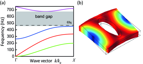
Figure 2: (Color online) (a) The phononic dispersion relation for the four lowest bands. The gray area denotes the phonon bandgap, and $\omega_{s}$ is the effective spin transition frequency. (b) The displacement pattern corresponding to the third band.

The coherent interaction between phononic crystal modes and electron spin states of a SiV center has been studied in our previous work arxiv-2019 (56). For the SiV center in diamond, the electronic ground state is split by the spin-orbit interaction and crystal strain into a lower branch (LB) and upper branch (UB) separated by $\Delta_{GS}=46$ GHz. In the presence of an external magnetic field, each branch is further broken to reveal two sublevels, i.e., $\{\left|g\right\rangle=\left|e_{-}\downarrow\right\rangle,\left|e\right\rangle=\left|e_{+}\uparrow\right\rangle\}$ and $\{\left|f\right\rangle=\left|e_{+}\downarrow\right\rangle,\left|d\right\rangle=\left|e_{-}\uparrow\right\rangle\}$, as show in Fig. $1(b)$, where $\left|e_{\pm}\right\rangle$ are eigenstates of the orbital angular momentum operator. When the transition frequency of the spin state is tunned close to the phononic band edge, we obtain the strong strain coupling between the SiV center and the phononic crystal mode. Applying a microwave driving field $\Omega$ to couple the states $\left|e\right\rangle$ and $\left|f\right\rangle$ and define appropriate detunings, the spin-phonon Hamiltonian can be mapped to the Jaynes-Cummings model, namely

$$H_{s-p}=\sum_{k}\hbar\omega_{k}a_{k}^{\dagger}a_{k}+\hbar\omega_{s}\sigma_{ee}+\underset{k}{\sum}\hbar g(a_{k}\sigma_{eg}e^{ikx_{0}}+H.c.),$$ (1)

where $\sigma_{eg}=\left|e\right\rangle\left\langle g\right|$, $\omega_{s}$ is the effective spin transition frequency, and $g$ is the effective spin-phonon coupling strength. Here, we assume that the defect center is only coupled to a single band of the phononic crystal, so the index $n$ can be omitted. In Figure. $2$, we numerically simulated the mechanical band structure and displacement pattern of one unit cell by finite element method (FEM), which is performed with the COMSOL Multiphysics software. By designing the parameters of the phononic crystal, the spin transition frequency is exactly lies within a phononic bandgap.

For a single excitation in the system, there exists a bound state $|\psi_{b}\rangle=\cos\theta|0\rangle|e\rangle+\sin\theta|1\rangle|g\rangle$ within the phononic bandgap. Here $|0\rangle$ is the vacuum state of the phonon mode, and $|1\rangle=\int dkc_{k}a_{k}^{\dagger}|0\rangle$ is single excitation state for the phonon modes. The bound state satisfies the eigenvalue equation $H_{s-p}|\psi_{b}\rangle=\hbar\omega_{b}|\psi_{b}\rangle$, where $\omega_{b}$ is the corresponding eigenfrequency. Based on the eigenvalue equation, the phononic spatial mode has the following form

$$\varepsilon(x)=\int dkc_{k}Q_{k}(x)=\sqrt{\frac{2\pi}{L_{c}}}e^{-|x-x_{0}|/L_{c}}Q_{k_{0}}(x),$$ (2)

that is the phononic part of the bound state is exponentially localized around the spin, with $L_{c}$ the localized length of the phononic wavefunction.

In the following, we study the interaction between phononic crystal waveguide modes and an array of SiV spins. Here we assume that the SiV centers are equally coupled to the phononic mode near the band gap, and the direct spin-spin interaction can be neglected, since it is excessively week compared with the spin-phonon interaction. Thus the interaction Hamiltonian between the defect spins and phonon modes can be expressed as

$$H_{s-s}=\sum_{j,k}\hbar g(a_{k}\sigma_{eg}^{j}e^{i\delta_{k}t+ikx_{j}}+H.c.),$$ (3)

with $\delta_{k}=\omega_{s}-\omega_{k}$. Assuming the large detuning regime, $\delta_{k}\gg g$, we can adiabatically eliminate the phonon modes cjp-85-625 (68), and then get the effective Hamiltonian

$$H_{s-s}=\overset{2N}{\sum_{i,j=1}}\hbar\mathcal{M}_{i,j}(\sigma_{eg}^{i}\sigma_{ge}^{j}+H.c.),$$ (4)

where

$$\mathcal{M}_{i,j}=\frac{g_{c}^{2}}{2\Delta_{BE}}e^{-|x_{i}-x_{j}|/L_{c}}$$ (5)

denotes the effective spin-spin interaction, $g_{c}=g\sqrt{2\pi a/L_{c}}$ is the the band gap engineered spin-phonon coupling strength, and $\Delta_{BE}=\omega_{s}-\omega_{BE}$, with $\omega_{BE}$ the phononic band edge frequency. Note that different from the conventional dipole-dipole interaction mediated by a mechanical resonator or waveguide, the band-gap mediated spin-spin interaction is decay exponentially with the distance between spins. The detailed derivation can be found in Ref. arxiv-2019 (56).

II.2 The Periodic driving

The periodic driving is known to render effective Hamiltonian in which specific terms can be adiabatically eliminated. Driving a quantum system periodically in time can profoundly alter its long-time dynamics and trigger topological order prx-4-031027 (69). As for the SiV color center in diamond, the electric structure is comprised of spin and orbital degrees of freedom. Considering the spin-orbit interaction and strain environment, there are four sublevels combined by orbital and spin components, as shown in Fig. $1(b)$. The spin-flip transitions are allowed between ground-state levels of opposite electronic spin in the SiV center. Thus, we can define the two lower sublevels $(|g\rangle,|e\rangle)$ as a spin qubit, and apply the extra driving fields to the SiV centers prl-119-210401 (16)

$$H_{d}=\frac{\hbar\Omega_{d}}{2}\overset{2N}{\sum_{j=1}}\sigma_{j}^{z}+\frac{\hbar\eta\omega_{d}}{2}\cos(\omega_{d}t)\overset{2N}{\sum_{j=1}}\cos(\Delta kx_{j}+\omega_{d}t)\sigma_{j}^{z},$$ (6)

with the Pauli operator component $\sigma_{j}^{z}=|e\rangle_{j}\langle e|-|g\rangle_{j}\langle g|$. The first term describes a transverse microwave field. The second term represents a periodically driving, which can be realized by a time-dependent standing wave with frequency $\omega_{d}$ and wavevector $\Delta k$ along the array direction. $\eta$ is the dimensionless coupling strength, $x_{j}=d_{0}j$ is the equilibrium position of the spin, with $d_{0}$ the distance between the evenly spaced spins.

Now we transform the total Hamiltonian $H_{tot}=H_{s-s}+H_{d}$ into the interaction picture, with the unitary operator $U(t)=e^{-i\int_{0}^{t}d\tau H_{d}/\hbar}$. Here we note that $H_{d}$ is time-dependent fields. In the interaction picture,

$$\sigma_{eg}^{j} \rightarrow e^{i\Delta_{j}(t)\sigma_{j}^{z}}\sigma_{eg}^{j}e^{-i\Delta_{j}(t)\sigma_{j}^{z}}=\sigma_{eg}^{j}e^{2i\Delta_{j}(t)},$$

$$\sigma_{ge}^{j} \rightarrow e^{i\Delta_{j}(t)\sigma_{j}^{z}}\sigma_{ge}^{j}e^{-i\Delta_{j}(t)\sigma_{j}^{z}}=\sigma_{ge}^{j}e^{-2i\Delta_{j}(t)},$$ (7)

with

$$\Delta_{j}(t)=\frac{\Omega_{d}}{2}t+\frac{\eta\omega_{d}}{2}\cos(\Delta kx_{j}+\omega_{d}t)\sin(\omega_{d}t).$$ (8)

To simplify the results, we use the trigonometric identity $\cos A-\cos B=-2\sin(\frac{A+B}{2})\sin(\frac{A-B}{2})$ and Jacobi-Anger expansion $e^{iz\sin\phi}=\sum_{n=-\infty}^{\infty}B_{n}(z)e^{in\phi}$, where $B_{n}(z)$ is the Bessel functions of the first kind. Here we consider the limit $\omega_{d}\gg\mathcal{M}_{i,j}$. Under the rotating wave approximation, only terms that contain zero-order Bessel functions are remained, ie., $n=0$. Then the interaction Hamiltonian has the form

$$H_{tot}=\overset{2N}{\sum_{i,j=1}}\hbar\mathcal{M}_{i,j}J_{i,j}(\sigma_{eg}^{i}\sigma_{ge}^{j}+\sigma_{ge}^{i}\sigma_{eg}^{j}),$$ (9)

with

$$J_{i,j}=B_{0}(2\eta\sin(\frac{\pi}{4}(i+j)+\omega_{d}t)\sin\frac{\pi}{4}(i-j)).$$ (10)

To achieve the periodic coupling, here we fixed $\Delta k=\frac{\pi}{2d_{0}}$. According to the expression of Bessel function, we can get $J_{j,j+1}=J_{j+2,j+3}$. Furthermore, for the nearest-neighbor spins, the interaction strength $\mathcal{M}=\frac{g_{c}^{2}}{2\Delta_{BE}}e^{-d_{0}/L_{c}}$ with $d_{0}=\left|x_{i}-x_{i+1}\right|$. If we define

$$\delta=\frac{J_{2,3}-J_{1,2}}{J_{2,3}+J_{1,2}},$$ (11)

then the Hamiltonian $H_{tot}$ can be rewritten as

$$H_{tot}=\overset{2N}{\sum_{j=1}}\hbar J\sigma_{eg}^{j}\sigma_{ge}^{j+1}+H.c.,$$ (12)

with $J=\mathcal{M}[1+(-1)^{j}\delta]$. As sketched in Fig. $3(a)$, two possible coupling rates $J_{1}=\mathcal{M}(1-\delta)$ and $J_{2}=\mathcal{M}(1+\delta)$ are staggered along the array. To better describe the physical picture of Eq. $(12)$, we rewrite the coupling pattern of the Fig. $3(a)$ as

$$H_{tot}=\overset{2N}{\underset{j\in odd}{\sum}}\hbar J_{1}\sigma_{eg}^{j}\sigma_{ge}^{j+1}+\overset{2N}{\underset{j\in even}{\sum}}\hbar J_{2}\sigma_{eg}^{j}\sigma_{ge}^{j+1}+H.c..$$ (13)

Considering this periodic spin-spin interaction, we group the nearest-neighbor spins with the coupling strength $J_{1}$ into a unit cell, where odd spins are labeled as $A_{n}$ and even spins are labeled as $B_{n}$, $n=1,2,\ldots,N$. The interaction Hamiltonian becomes

$$H_{SSH}=\overset{N}{\underset{n=1}{\sum}}\hbar(J_{1}A_{n}^{\dagger}B_{n}+J_{2}B_{n}^{\dagger}A_{n+1}+H.c.),$$ (14)

with

$$A_{n} = \sigma_{ge}^{j},\ j=1,3,5,7\ldots,$$

$$B_{n} = \sigma_{ge}^{j},\ j=2,4,6,8\ldots.$$ (15)

This is the well-known one-dimensional SSH model, where $J_{1}$ and $J_{2}$ describe the intracell and intercell hoppings, respectively. The SSH model occurs naturally in many solid-state systems, e.g., polyacetylene, which is known as the simplest instances of a topological insulator. Likewise, the staggering of the hopping amplitudes has also been realized in several other quantum systems, such as optical cavities, trapped-ions and superconducting circuits prl-119-210401 (16, 17). In our work, phononic crystals possess unique band gap structures, which provide stronger spin-phonon interactions due to the much tighter confinement of the mediating phonon. Moreover, periodic driving fields enable the highly controllable SSH model in the color center arrays.

II.3 Topological characters

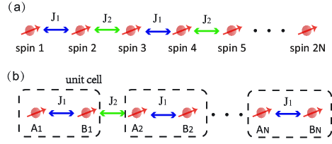
Figure 3: (Color online) (a) Schematic diagram for the array of coupled SiV spins with staggering coupling strength $J_{1}$ and $J_{2}$. (b) The schematic diagram of Hamiltonian $H_{SSH}$, $J_{1}$ and $J_{2}$ describe the intracell and intercell hoppings, respectively.

The SSH model has served as a prototypical example of the one-dimensional system supporting topological character. To explore topological features of the effective spin-spin system, we convert $H_{tot}$ to the momentum space. Considering periodic boundary conditions, we can make the Fourier transformation

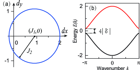
Figure 4: (Color online) (a) The path of the endpoints of the vector $d_{k}$ for $\delta=0.1$. (b) The corresponding dispersion relations of the SSH model in momentum space. The other parameter is $\mathcal{M}=1$.

$$A_{n} = \frac{1}{\sqrt{N}}\sum_{k}e^{ink}A_{k},$$

$$B_{n} = \frac{1}{\sqrt{N}}\sum_{k}e^{ink}B_{k},$$ (16)

where $k=2\pi m/N(m=1,2,...,N)$ is the wavenumber in the first Brillouin zone, and $A_{k}$ and $B_{k}$ are the momentum space operators. Defining the unitary operator $\psi_{k}=\left(\begin{array}[]{cc}A_{k}&B_{k}\end{array}\right)^{T}$, the Hamiltonian $H_{SSH}$ can be rewritten as

$$H_{SSH}=\sum_{k}\psi_{k}^{\dagger}H(k)\psi_{k},$$ (17)

where

$$H(k)=\hbar\left(\begin{array}[]{cc}0&f(k)\\ f^{\ast}(k)&0\end{array}\right)$$ (18)

is the momentum-space Hamiltonian. Here, $f(k)=d(k)\cdot\sigma$ describes the coupling between $A$ and $B$ spins in momentum space, $\sigma=(\sigma_{x},\sigma_{y},\sigma_{z})$ is the Pauli matrix, and $d(k)$ denotes a three-dimensional vector field. For the generalized SSH model, we have

$$d_{x}(k) = J_{1}+J_{2}\cos k,$$

$$d_{y}(k) = J_{2}\sin k,$$

$$d_{z}(k) = 0.$$ (19)

We show the path of the endpoints of the vector $d(k)$ for different $\delta$ in Fig. $4(a)$. As the wavenumber runs through the Brillouin zone $k=0\rightarrow 2\pi$, the path depicted by the endpoint of $d(k)$ is a closed circle of radius $J_{2}$ on the $dx$-$dy$ plane, centered at $(J_{1},0)$.

Now we proceed to investigate the energy spectrum of the SSH model in momentum space. Sloving the eigenvalue equation

$$H(k)\psi_{k}=E(k)\psi_{k},$$ (20)

we get

$$E(k)=\pm\hbar\left|J_{1}+J_{2}e^{-ik}\right|.$$ (21)

Furthermore, the eigenenergy can be expressed as $E(k)=\pm\hbar\mathcal{M}\sqrt{2(1+\delta^{2})+2(1-\delta^{2})\cos k}$. Figs. $4(b)$ shows the corresponding dispersion relations for different $\delta$: (i) for the general case with $\delta\neq 0$, the spin-spin interactions have a chiral symmetry, such that all eigenmodes can be grouped in chiral symmetric pair with opposite energies. Thus, the engrgy spectrum is split into two branches, and there exist a band gap $2\Delta E(k)$ locates at $k=\pi$, with

$$\Delta E(k)=\min E(k)=2\left|\delta\right|.$$ (22)

(ii) for the case with $\delta=0$, i.e., the spin-spin hopping rate is a constant, the band gap is closed, which recovers the normal 1D tight-binding model.

From Eq. $(21)$ we conclude that, the system with $\delta<0$ and $\delta>0$ share the identical band structure, but they are topologically inequivalent. As a topological invariant, the Winding number can be used to characterize the topological properties of the one-dimensional system. According to the above derivation, the energy bands of the Hamiltonian $E(k)$ is determined by the vector field $d(k)$. Hence, the Winding number can be conveniently expressed as

$$\mathcal{W}=\frac{1}{2\pi}\int_{0}^{2\pi}(n_{x}\partial_{k}n_{y}-n_{y}\partial_{k}n_{x})dk,$$ (23)

where $(n_{x},n_{y})=(d_{x},d_{y})/\sqrt{d_{x}^{2}+d_{y}^{2}}$ is the normalized vector, and $\partial_{k}$ is the partial derivative with respect to $k$. So we can obtain that the Winding number is either $0$ or $1$. In the case $\delta<0$, the Winding number $\mathcal{W}=0$, the system is topological trivial. While in the case $\delta>0$, the Winding number $\mathcal{W}=1$, the system has a topological nontrivial phase.Thus, at the critical point $\delta=0$, one can implement the topological phase transitions.

III Simulation of the 2D SSH model

The Su-Schrieffer-Heeger model inherently possesses topological features, providing an effective pattern to study topological phenomena in quantum systems. It is naturally expected to investigate the SSH model in high-dimensional quantum systems and develop interesting applications in quantum information processing. For phononic crystals, owing to the advantage of the scalable nature of nanofabrication, the extension to high-dimensional cases is experimentally feasible and has been extensively studied. In this section, we focus on the 2D SSH model and relevant topological characters in this spin-phononic system.

III.1 The setup

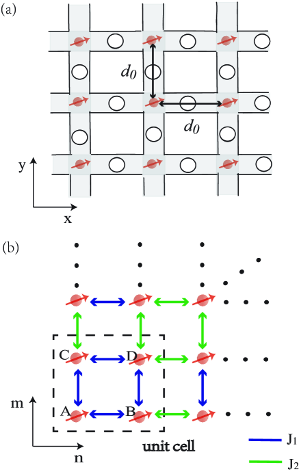
Figure 5: (Color online) (a) Schematics of the two-dimensional phononic network studied in this work. SiV spins are located at the nodes of the phononic structure. $d_{0}$ is the distance between two adjacent spins. (b) The schematic diagram of the Hamiltonian $H_{SSH}^{(2D)}$. There are four spins in each unit cell, labeled as {$A,B,C,D$}, with $J_{1}$ and $J_{2}$ described the intracell and intercell hoppings, respectively.

Here we consider a phononic network with square lattices on the $x$-$y$ plane, with $2N\times 2N$ SiV spins located separately at the nodes of the phononic structure, as depicted in Fig. $5(a)$. Based on the coupling of SiV center arrays to the 1D phononic crystal, we thereby obtain the phononic mediated spin-spin interactions in this 2D phononic network

$$H_{s-s}^{(2D)} = H_{s-s}^{(x)}+H_{s-s}^{(y)},$$

$$H_{s-s}^{(x)} = \overset{2N}{\sum_{l=1}}\overset{2N}{\sum_{i,j=1}}\hbar(\mathcal{M}_{i,j}\sigma_{eg}^{(i,l)}\sigma_{ge}^{(j,l)}+H.c.),$$

$$H_{s-s}^{(y)} = \overset{2N}{\sum_{j=1}}\overset{2N}{\sum_{k,l=1}}\hbar(\mathcal{M}_{k,l}\sigma_{eg}^{(j,k)}\sigma_{ge}^{(j,l)}+H.c.),$$ (24)

where $H_{s-s}^{(x)}$ and $H_{s-s}^{(y)}$ describe the effective spin-spin interactions in the $x$ and $y$ directions, respectively, and $\mathcal{M}_{i,j},\mathcal{M}_{k,l}$ are the corresponding phonon mediated spin-spin hopping rates.

III.2 The periodic driving

According to the 1D SSH model, we can obtain a topological nontrivial system by applying a specific periodic driving to the SiV spins. For the 2D case, we consider adding two mutually perpendicular microwave fields to the color center arrays prb-95-205125 (70). The first one is a time-dependent microwave field of frequency $\omega_{d}$ in the $x$ direction. The other is an identical periodic driving in the $y$ direction. These two periodic driving terms have the form

$$H_{d}^{(x)} = \frac{\hbar\eta\omega_{d}}{2}\cos(\omega_{d}t)\overset{2N}{\sum_{l=1}}\overset{2N}{\sum_{j=1}}\cos(\Delta k_{x}x_{j}+\omega_{d}t)\sigma_{j,l}^{z},$$

$$H_{d}^{(y)} = \frac{\hbar\eta\omega_{d}}{2}\cos(\omega_{d}t)\overset{2N}{\sum_{j=1}}\overset{2N}{\sum_{l=1}}\cos(\Delta k_{y}y_{l}+\omega_{d}t)\sigma_{j,l}^{z},$$ (25)

where $\Delta{k}_{x}$ and $\Delta{k}_{y}$ are the wavevectors along the spin array direction. $(x_{j},y_{l})$ describes the spin position in the phononic network, here $x_{j}=d_{0}j$ and $y_{l}=d_{0}l$. In addition, for the SiV spins, we apply an additional transverse microwave driving $H_{d}^{0}=\frac{\hbar\Omega_{d}}{2}\sum_{j,l}\sigma_{j,l}^{z}$, which enables the external driving of spins to have the same form as Eq. $(6)$.

For the periodic driving spin arrays along the $x$ direction, the total Hamiltonian is given by

$$H_{tot}^{(x)}=H_{s-s}^{(x)}+H_{d}^{(x)}+H_{d}^{0}.$$ (26)

In the interaction picture, we introduce the unitary operator $U(t)=e^{-i\int_{0}^{t}d\tau(H_{d}^{(x)}+H_{d}^{0})/\hbar}$. After the unitary transformation, we can obtain

$$\sigma_{eg}^{(j,l)} \rightarrow \sigma_{eg}^{(j,l)}e^{2i\Delta_{j}(t)},$$

$$\sigma_{ge}^{(j,l)} \rightarrow \sigma_{ge}^{(j,l)}e^{-2i\Delta_{j}(t)},$$ (27)

with

$$\Delta_{j}(t)=\frac{\Omega_{d}}{2}t+\frac{\eta\omega_{d}}{2}\cos(\Delta k_{x}x_{j}+\omega_{d}t)\sin(\omega_{d}t).$$ (28)

In the regime $\omega_{d}\gg\mathcal{M}_{i,j}$, we proceed to renormalize the spin-spin hopping amplitudes with the zero-order Bessel function, and obtain the interaction Hamiltonian

$$H_{tot}^{(x)}=\overset{2N}{\sum_{l=1}}\overset{2N}{\sum_{i,j=1}}\hbar\mathcal{M}_{i,j}J_{i,j}(\sigma_{eg}^{i,l}\sigma_{ge}^{j,l}+\sigma_{ge}^{i,l}\sigma_{eg}^{j,l}),$$ (29)

with

$$J_{i,j}=B_{0}(2\eta\sin(\frac{\pi}{4}(i+j)+\omega_{d}t)\sin\frac{\pi}{4}(i-j)).$$ (30)

Similar to the discussion in the $x$ direction, the Hamiltonian in the $y$ direction can be written as

$$H_{tot}^{(y)}=H_{s-s}^{(y)}+H_{d}^{(y)}+H_{d}^{0}.$$ (31)

In the regime $\omega_{d}\gg\mathcal{M}_{k,l}$, we obtain the effective spin-spin interaction along the $y$ coordinate

$$H_{tot}^{(y)}=\overset{2N}{\sum_{j=1}}\overset{2N}{\sum_{k,l=1}}\hbar\mathcal{M}_{k,l}J_{k,l}(\sigma_{eg}^{(j,k)}\sigma_{ge}^{(j,l)}+\sigma_{ge}^{(j,k)}\sigma_{eg}^{(j,l)}),$$ (32)

with

$$J_{k,l}=B_{0}(2\eta\sin(\frac{\pi}{4}(k+l)+\omega_{d}t)\sin\frac{\pi}{4}(k-l)).$$ (33)

To simplify the model, here we assumed $\Delta{k}_{x}=\Delta{k}_{y}=\frac{\pi}{2d_{0}}$. In this case, according to the definition of $\delta$ given in Eq. $(11)$, we have

$$\delta_{x}=\delta_{y}=\delta.$$ (34)

For the 2D spin-spin interactions, the total Hamiltonian can be written as

$$H_{tot}^{(2D)}=\overset{2N}{\sum_{j=1}}\overset{2N}{\sum_{l=1}}\hbar(J_{x}\sigma_{eg}^{(j,l)}\sigma_{ge}^{(j+1,l)}+J_{y}\sigma_{eg}^{(j,l)}\sigma_{ge}^{(j,l+1)}+H.c.),$$ (35)

with $J_{x}=\mathcal{M}[1+(-1)^{j}\delta]$ and $J_{y}=\mathcal{M}[1+(-1)^{l}\delta]$. Therefore, there are two possible coupling constants $J_{1}$ and $J_{2}$ staggered in the $x$ and $y$ directions.

In the following, analogous to Eq. $(14)$, we group the nearest-neighbor spins with the coupling strength $J_{1}$ into a unit cell. Then we get a two-dimensional system with $N\times N$ unit cells. As shown in Fig. $5(b)$, there are four spins in a unit cell, which are labeled as {$A,B,C,D$}, respectively. Then we can rewrite the two-dimensional Hamiltonian as

$$H_{SSH}^{(2D)} = \overset{N}{\sum_{n=1}}\overset{N}{\sum_{m=1}}\hbar[J_{1}(A_{n,m}^{\dagger}B_{n,m}+A_{n,m}^{\dagger}C_{n,m}$$ (36)

$$+B_{n,m}^{\dagger}D_{n,m}+C_{n,m}^{\dagger}D_{n,m}+H.c.)$$

$$+J_{2}(A_{n+1,m}^{\dagger}B_{n,m}+A_{n,m+1}^{\dagger}C_{n,m}$$

$$+B_{n,m+1}^{\dagger}D_{n,m}+C_{n+1,m}^{\dagger}D_{n,m}+H.c.)].$$

This is the generalized two-dimensional SSH model prappl-12-034014 (19, 20, 21). For simplicity, here we introduce $(n,m)$ to describe the position of each unit cell, $n,m=1,2,\ldots,N$.

III.3 Topological characters

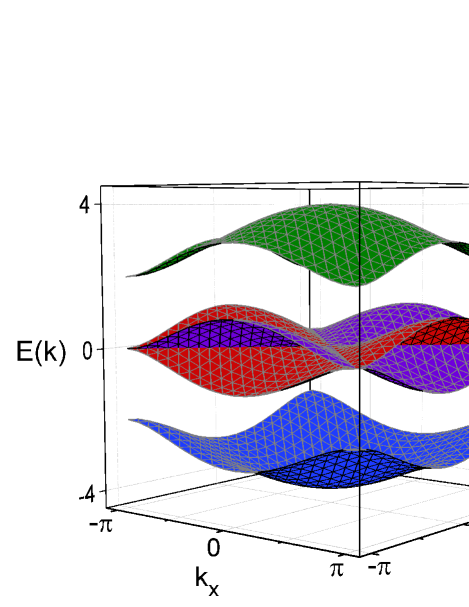
Figure 6: (Color online) Band structure of the 2D SSH model as a function of $k_{x}$ and $k_{y}$, with $\delta=0.5$. The energy spectrum has four branches.

To explore the topological features of the two-dimensional SSH model, we proceed to convert $H_{tot}$ to the momentum space. As displayed in Fig. 5, four nearest-neighbor SiV spins with the coupling strength $J_{1}$ form a unit cell, which is a square lattice geometry. The distance between two adjacent spins is $d_{0}$. Thus, the primitive translation vectors are $\textbf{a${}_{1}$}=(2d_{0},0)$ and $\textbf{a${}_{2}$}=(0,2d_{0})$, and the corresponding reciprocal lattice vectors are $\textbf{b${}_{1}$}=(\pi/d_{0},0)$ and $\textbf{b${}_{2}$}=(0,\pi/d_{0})$. This two-dimensional spin-spin interaction obeys $C_{4v}$ point group symmetry of the Bravais lattice.

Analogous to the one-dimensional case, here we consider periodic boundary conditions along both the $x$ and $y$ directions. Applying the Fourier transformation to the four spins in a unit cell

$$A_{n,m} = \frac{1}{\sqrt{N}}\sum_{\textbf{k}}e^{i(k_{x}n+k_{y}m)}A_{\textbf{k}},$$

$$B_{n,m} = \frac{1}{\sqrt{N}}\sum_{\textbf{k}}e^{i(k_{x}n+k_{y}m)}B_{\textbf{k}},$$

$$C_{n,m} = \frac{1}{\sqrt{N}}\sum_{\textbf{k}}e^{i(k_{x}n+k_{y}m)}C_{\textbf{k}},$$

$$D_{n,m} = \frac{1}{\sqrt{N}}\sum_{\textbf{k}}e^{i(k_{x}n+k_{y}m)}D_{\textbf{k}},$$ (37)

where $\textbf{k}=(k_{x},k_{y})$ is the wavenumber in the first Brillouin zone. If we define the unitary operator $\psi_{\textbf{k}}=\left(\begin{array}[]{cccc}A_{\textbf{k}}&B_{\textbf{k}}&C_{\textbf{k}}&D_{\textbf{k}}\end{array}\right)^{T}$, the two-dimensional SSH Hamiltonian can be rewritten as

$$H_{SSH}^{(2D)}=\sum_{\textbf{k}}\psi_{\textbf{k}}^{\dagger}H(\textbf{k})\psi_{\textbf{k}}.$$ (38)

Then we obtain $4\times 4$ matrix form of the Hamiltonian in the k-space

$$H(\textbf{k})=\hbar\left(\begin{array}[]{cccc}0&f(k_{x})&f(k_{y})&0\\ f^{\ast}(k_{x})&0&0&f(k_{y})\\ f^{\ast}(k_{y})&0&0&f(k_{x})\\ 0&f^{\ast}(k_{y})&f^{\ast}(k_{x})&0\end{array}\right).$$ (39)

$f(k_{x})=J_{1}+J_{2}e^{-ik_{x}}$ describes the spin-spin couplings in the $x$ direction, i.e., $A$ $\leftrightarrow$ $B$ and $C$ $\leftrightarrow$ $D$. While $f(k_{y})=J_{1}+J_{2}e^{-ik_{y}}$ represents the spin-spin couplings in the $y$ direction, i.e., $A$ $\leftrightarrow$ $C$ and $B$ $\leftrightarrow$ $D$.

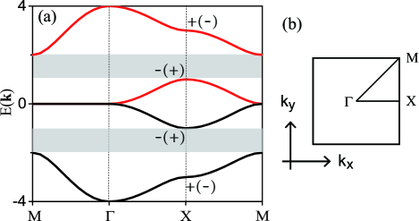
Figure 7: (Color online) (a) Dispersion relation along the path $M\rightarrow\Gamma\rightarrow X\rightarrow M$ in the first Brillouin zone. “$\pm$” means the parity of the eigenstates under $\pi$ rotation. The gray area denotes the energy band gap. Note that the band gap will be vanished if $\delta=0$. Here $\delta=0.5$.(b) First Brillouin zone of the squire lattice.

We now study the dispersion relation of the 2D SSH model. Solving the eigenvalue equation

$$H(\textbf{k})\psi_{\textbf{k}}=E(\textbf{k})\psi_{\textbf{k}},$$ (40)

we obtain

$$E(\textbf{k})=\epsilon_{x}\hbar\left|J_{1}+J_{2}e^{-ik_{x}}\right|+\epsilon_{y}\hbar\left|J_{1}+J_{2}e^{-ik_{y}}\right|,$$ (41)

with $\epsilon_{x}=\epsilon_{y}=\pm 1$. In Figure. $6$, we numerically calculate the band structure of the 2D SSH model in momentum space. The energy spectrum contains four bands: one around $E(\textbf{k})=4$, the symmetric one around $E(\textbf{k})=-4$, and a pair of symmetric bands around $E(\textbf{k})=0$.

In addition, we simulate the dispersion relation in the first Brillouin zone. As shown in Fig. $7(a)$, the four energy bands can be grouped as: two symmetric bands with opposite energies, and the middle pair degenerate at $C_{4v}$ invariant points. There are two equal energy band gaps, with the width $\Delta E(\mathbf{k})=2\left|\delta\right|$. According to Eq. $(41)$, the system has the identical band structure if we swap the coupling rates $J_{1}$ and $J_{2}$, which is the same as the one-dimensional case. However, for the 2D SSH model, the eigenstates of the system are qualitatively different. At the point of $X$, the wave functions possess opposite parities for swapped $J_{1}$ and $J_{2}$. In Fig. $7(a)$, we label the opposite parities of the eigenstates as “$+$” and “$-$”, respectively.

For the 1D SSH model, the energy band is closed when $\delta=0$. In this case, one can implement topological phase transitions. Inspired by this result, we continue to explore the topological phase of the 2D SSH model. In order to exactly characterize the topological nontrivial phase of the 2D SSH model, we introduce topological invariant Chern number $\mathcal{C}=(C_{x},C_{y})$ rmp-82-1959 (71), with

$$\mathcal{C}=\frac{1}{2\pi}\int_{BZ}dk_{x}dk_{y}\textbf{Tr}[A(\textbf{k})].$$ (42)

Here, $A(\textbf{k})=i\psi_{\textbf{k}}^{\dagger}\partial_{\textbf{k}}\psi_{\textbf{k}}$ is the non-Abelian Berry connection, and the integration is performed over the first Brillouin zone (BZ). Due to the $C_{4v}$ point group symmetry, we obtain $C_{x}=C_{y}$ in the 2D SSH system. In the case $\delta>0$, the Chern number $\mathcal{C}=(1/2,1/2)$, which implies that the system has a topological nontrivial phase. However, in the case $\delta<0$, the Chern number $\mathcal{C}=(0,0)$, which correspondings to the topological trivial case. Therefore, it is feasible to realize the topological phase transition in the 2D SSH system by modulating the periodic driving.

IV Quantum state transfer via the topological edge states

Long-range quantum state transfer is central to the study of time-evolving quantum systems rmp-70-1003 (72, 73, 74). As discussed above, applying a suitable periodic driving field to the SiV centers, the phononic band-gap mediated spin-spin interactions can be mapped to the SSH-type Hamiltonian. In the topological regime, we can obtain the obvious nontrivial edge states at the boundaries of the spin arrays. In this section, we take the 1D SSH as an example to show how quantum state can be transferred with high fidelity via the topological edge states.

IV.1 Edge states

The existence of edge states at the boundary is a distinguished feature for topological insulator states prl-89-077002 (75). In the following, we will discuss how to obtain the edge states in this spin-phononic system. We look for the zero energy state in the 1D SSH model. Here we introduce the single-excited state $|n_{\alpha}\rangle=\alpha_{n}^{\dagger}|ggg...\rangle$ $(\alpha=A,B)$, which describes the spin at the $\alpha$ sites of the $n$th cell excited to the state $|e\rangle$, while other spins stay in the ground state $|g\rangle$. In the single-excited state subspace, the Hamiltonian $H_{SSH}$ has the form

$$H_{SSH}=\overset{N}{\underset{n=1}{\sum}}\hbar(J_{1}|n_{A}\rangle\left\langle n_{B}\right|+J_{2}|n_{B}\rangle\left\langle(n+1)_{A}\right|+H.c.).$$ (43)

Hence, we can get the the zero-energy eigenstates by sloving

$$H_{SSH}\overset{N}{\underset{n=1}{\sum}}(a_{n}|n_{A}\rangle+b_{n}|n_{B}\rangle)=0,$$ (44)

where $a_{n}$ and $b_{n}$ are the amplitudes of occupying probability in the $n$th cell. There are $2N$ equations for the amplitudes $a_{n}$ and $b_{n}$,

$$J_{1}a_{n}+J_{2}a_{n+1} = 0$$

$$J_{2}b_{n}+J_{1}b_{n+1} = 0.$$ (45)

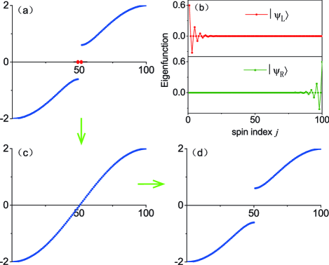
Figure 8: (Color online) The single-excited energy spectrum of Hamiltonian $H_{SSH}$ for different $\delta$: (a) $\delta=0.3$, (c) $\delta=0$, (d) $\delta=-0.3$. (b) Wavefunction of the left and right edge states versus spin index $j$ with $\delta=0.3$. The other parameters are $\mathcal{M}=1$ and $N=100$.

It should be noted that, for the boundaries, $b_{1}=a_{N}=0$. In the thermodynamic limit, $N\rightarrow\infty$, if we consider the case of $J_{1}<J_{2}$, we can obtain the left and right zero-energy edge states as

$$|\psi_{L}\rangle = \overset{N}{\underset{n=1}{\sum}}a_{1}e^{-(n-1)/\xi}|n_{A}\rangle,$$

$$|\psi_{R}\rangle = \overset{N}{\underset{n=1}{\sum}}b_{N}e^{(n-N)/\xi}|n_{B}\rangle,$$ (46)

where $\xi=1/\log(J_{1}/J_{2})$ is the localization length. When the ratio $J_{2}/J_{1}$ becomes appreciably large, the wavefunction will almost be confined at the first and last spins.

In order to verify the model, we numerically simulate the eigenvalues of the system in Figs. $8(a)$, $(c)$ and $(d)$. For $\delta>0$, i.e., $J_{1}<J_{2}$, there exists a energy band gap and two zero-energy eigenvalues of the system. When $\delta=0$, the gap is vanished. For $\delta<0$, the gap opens again but no gapless modes appear. Correspondingly, we show the zero-energy edge states in Fig. $8(b)$. We see that the wavefunctions are localized exponentially in the vicinity of the array edges, which is consistent with the theoretical result.

As shown in Fig. $8(b)$, we can also find that the left (right) edge states only exist in the odd (even) spins, which is the consequence of chiral symmetry lecture-2016 (11). In general, we say that a system with Hamiltonian $H$ has chiral symmetry, if $\Gamma H\Gamma^{\dagger}=-H$, $\Gamma$ is the chiral symmetry operator. Here we define two orthogonal projection operators,

$$\mathcal{P}_{A}=\frac{1}{2}(I+\Gamma),\mathcal{P}_{B}=\frac{1}{2}(I-\Gamma),$$ (47)

where $I$ is the identity operator in the Hilbert space, $\mathcal{P}_{A}$ and $\mathcal{P}_{B}$ signify the projection to the spins at $A$ and $B$ sites, respectively. Note that $\mathcal{P}_{A}+\mathcal{P}_{B}=1$ and $\mathcal{P}_{A}\mathcal{P}_{B}=0$. The Hamiltonian of the SSH model is bipartite: there are no transitions between spins with the same label ($A$ or $B$), i.e., $\mathcal{P}_{A}H_{SSH}\mathcal{P}_{A}=\mathcal{P}_{B}H_{SSH}\mathcal{P}_{B}=0$. In fact, using the projectors $\mathcal{P}_{A}$ and $\mathcal{P}_{B}$ is an alternative and equivalent way of defining chiral symmetry. For the zero-energy eigenstates, we obtain

$$H_{SSH}\mathcal{P}_{A/B}|\psi_{n}\rangle=H_{SSH}(|\psi_{n}\rangle\pm\Gamma|\psi_{n}\rangle)=0.$$ (48)

The projected zero energy states are eigenstates of the chiral symmetry operator $\Gamma$, and therefore are chiral symmetric partners of themselves. It is for this reason that the edge states are supported only by odd or even spins.

IV.2 Quantum state transfer

In the following, we present the applications of this spin-phononic system and show that the topological edge states can be employed as a quantum channel between distance qubits. Since quantum information could be transferred directly between the boundary spins, the intermediate spins are virtually excited during the process, which ensures the robust quantum state transfer. Taking into account the coupling of the system with the environment in the Markovian approximation, the evolution of the system follows the master equation

$$\dot{\rho}=-\frac{i}{\hbar}[H_{SSH},\rho]+\overset{2N}{\sum_{j=1}}\gamma_{s}\mathcal{D}[\sigma_{j}^{z}]\rho,$$ (49)

with $\sigma_{j}^{z}=|e\rangle_{j}\langle e|-|g\rangle_{j}\langle g|$, $\gamma_{s}$ the spin dephasing rate of the single SiV centers, and $\mathcal{D}[O]\rho=O\rho O^{\dagger}-\frac{1}{2}\rho O^{\dagger}O-\frac{1}{2}O^{\dagger}O\rho$ for a given operator $O$.

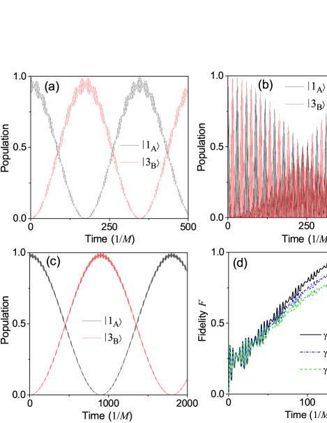
Figure 9: (Color online) Time evolution of the population of the two edge states. (a) $\delta=0.7$. (b) $\delta=-0.7$. (c) $\delta=0.82$. (d) Time evolution of the fidelity $F$ with different spin dephasing rate $\gamma_{s}$. The other parameters are $\mathcal{M}=1$ and $N=3$.

To verify the transfer of the edge states and evaluate the performance of this protocol, we numerically simulate the dynamics of the system by using the QuTiP library, as shown in Fig. $9$. Here we take $6$ spins as an example, i.e., $N=3$. As illustrated in Fig. $9(a)$, in the topological regime ($\delta>0$), we obtain the significant quantum state transfer between the two end spins. However, for the non-topological condition, i,e., $\delta<0$, no direct quantum state transfer can be seen, as shown in Fig. $9(b)$. In addition, we simulate the effect of different values of the parameter $\delta$ on quantum state transfer. Compared Fig. $9(a)$ with Fig. $9(c)$, we can see that the localization of the edge states is more obvious when $\delta$ takes a larger value, which is consistent with the theoretical results. At the same time, for larger $\delta$, the time for accomplishing quantum state transfer increases. It should be noted that the time required for the system to realize the quantum state transfer should be shorter than the coherence time of single SiV spins. Thus, when improving the value of $\delta$, we should consider the coherence time of the system as well. Note that we neglect the spin dephasing in Fig. 9(a)-(c).

We now discuss the impact of spin dephasing of SiV centers on quantum information transfer. Here we use fidelity to describe the performance of the state transfer, which is defined as

$$\mathcal{F}=\left\{Tr[(\sqrt{\rho(t_{f})}\rho(t_{i})\sqrt{\rho(t_{f})})]^{1/2}\right\}^{2}.$$ (50)

$\rho(t_{i})$ and $\rho(t_{f})$ denote the density operator for the initial and final state of the transfer process, respectively rmap-9-273 (76). In Fig. 9(d), we present the fidelity $\mathcal{F}$ as a function of time starting from the initial state $|1_{A}\rangle$. In the absence of spin dephasing, it is shown that, the system evolves to the final state $|3_{B}\rangle$ with a fidelity $\mathcal{F}\simeq 1$ (black solid line). This simulation result indicates that quantum state transfer are indeed realized between the two end spins. Moreover, we simulate time evolution of the fidelity taking into consideration of spin dephasing. As shown in Fig. 9(d), when setting the dephashing rate $\gamma_{s}=5\times 10^{-4}\mathcal{M}$, it is seen that the fidelity is about $0.91$. Furthermore, as the dephasing rate increases to $1\times 10^{-3}\mathcal{M}$, which is much closer to the realistic experimental conditions, the fidelity of this scheme can still reach $\mathcal{F}=0.84$ (green dash line). Therefore, our protocol can realize high fidelity quantum state transfer with feasible experimental parameters.

IV.3 Approximate solutions

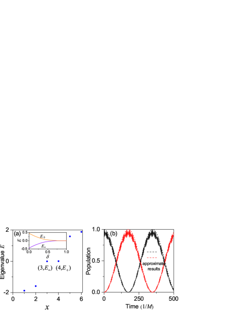
Figure 10: (Color online) (a) $E_{+}$ and $E_{-}$ are the eigenvalues of the two edge states, and $\delta=0.7$. The inset graph shows the eigenvalue $E$ as a function of $\delta$. (b) The comparison between the exact simulations and theoretical approximate results. Other parameters are the same as those in Fig. $9$.

In the following, we provide the comparison between our protocol and theoretical approximate results. According to Eq. $(46)$, if we assign appreciably large values to the ratio $J_{2}/J_{1}$, the zero-energy edge states will almost be confined at the first and end spins of the array. Here we assume the two edge states $\left|e_{+}\right\rangle$ and $\left|e_{-}\right\rangle$, and the corresponding energies $E_{+}$ and $E_{-}$ are shown in Fig. 10(a). Then we can consider

$$\left|1_{A}\right\rangle = \frac{1}{\sqrt{2}}(\left|e_{+}\right\rangle+\left|e_{-}\right\rangle),$$

$$\left|3_{B}\right\rangle = \frac{1}{\sqrt{2}}(\left|e_{+}\right\rangle-\left|e_{-}\right\rangle),$$ (51)

If the initial condition is $\left|\psi(0)\right\rangle=\left|1_{A}\right\rangle$, the time evolution of the quantum state follows

$$\left|\psi(t)\right\rangle=\frac{1}{\sqrt{2}}(e^{-iE_{+}t/\hbar}\left|e_{+}\right\rangle+e^{-iE_{-}t/\hbar}\left|e_{-}\right\rangle).$$ (52)

Then we can obtain the mean population of the two ends of the array, i.e., $\left\langle 1_{A}\right\rangle=(1+\cos(\omega_{0}t))/2$ and $\left\langle 3_{B}\right\rangle=(1-\cos(\omega_{0}t))/2$ with $\omega_{0}=(E_{+}-E_{-})/\hbar$. In Fig. $10(b)$, we plot the time evolution of the spin populations, and find the excellent match between our protocol and theoretical approximate results. It should be noted that, in non-topological regime, for the same initial condition, the state will be a superposition of more eigenstates and the particle will spread over the entire array.

V experimental consideration

In this work, we consider a spin-phononic crystal system, where arrays of SiV centers are coupled by the quantized phonon modes of diamond phononic crystals. Based on state-of-the-art nanofabrication techniques, several experiments have demonstrated the generation of color center arrays through ion implantation NL-10-3168 (77, 78). And the fabrication of nanoscale mechanical structures with diamond crystals has been realized experimentally, as proposed in Refs. opt-3-1404 (45, 66, 79). In general, the periodicity of a phononic crystal structure is characterised by periodic air holes etched on the crystal, which yields the tunable phononic bands. Since the excellent scalability of phononic crystal structures, this SSH model is experimentally feasible when extending to the higher dimensional case.

For the diamond phononic crystal, the material properties are $E=1050$ GPa, $\nu=0.2$, and $\rho=3539$ kg/m³. The lattice constant and cross section of phononic crystal are $a=100$ nm and $A=100\times 20$ nm², while the semi-major and -minor axis of the elliptical holes are $15$ nm and $38$ nm, respectively. In this case, we get a phononic band edge frequency $\omega_{BE}/2\pi=44.933$ GHz, the ground state transition frequency of SiV center is about $46$ GHz, which is exactly located in a phononic bandgap, as shown in Fig. 2(a). The coupling between the SiV center and phononic crystal mode $k$ is given by $g_{k}=\frac{d}{v_{l}}\sqrt{\frac{\hbar\omega_{BE}}{2\pi\rho aA}}\xi(\vec{r})$ NJP-17-043011 (82, 83), where $d/2\pi\sim 1$ PHz is the strain sensitivity, and $v_{l}=1.71\times 10^{4}$ m/s is the speed of sound in diamond. $\xi(\vec{r})$ is the dimensionless strain distribution at the position of the SiV center $\vec{r}$, and here we assign $\xi(\vec{r})=1$ apl-87-043011 (84). Then we get the SiV-phononic coupling rate $g_{k}/2\pi\simeq 100$ MHz. In the large detuning regime, $g\sim 0.1g_{k}$, leading to the band gap engineered spin-phononic coupling rate $g_{c}=g\sqrt{2\pi a/L_{c}}\simeq 2\pi\times 25$ MHz.

For the SiV color center in diamond, the two lower sublevels $(|g\rangle,|e\rangle)$ can be defined as a spin qubit and coherently controlled by using microwave fields Natcomm-8-15579 (80, 81). Moreover, in high-strain regime, the magnetic dipole transition between the ground-state levels of SiV centers can be directly driven with microwaves, which is already experimentally performed prb-100-165428 (85). According to Eq. $(11)$, the definition of $\delta$ is derived from the periodic microwave driving. We can obtain different values of $\delta$ by adjusting parameters $\eta$ and $\omega_{d}$ of the periodic driving fields, which makes our model highly controllable and tunable.

At mK temperatures, the spin dephasing time of single SiV center is about $\gamma_{s}/2\pi=100$ Hz. As for phononic crystals, the mechanical quality factor is $Q\sim 10^{7}$, which can be achieved and further improved by using 2D phononic crystal shields prx-8-041027 (54). Thus we obtain the mechanical dampling rate $\gamma_{m}/2\pi=4.5$ kHz. In this setup, the band gap engineered spin-phononic coupling strength is $g_{c}/2\pi\simeq 25$ MHz, which considerably exceeds both $\gamma_{s}$ and $\gamma_{m}$, resulting in the strong strain interaction between the SiV centers and phonon crystal modes. For the nearest neighbour spins with $d_{0}=a$, the phononic band-gap mediated spin-spin interaction $\mathcal{M}=\frac{g_{c}^{2}}{2\Delta_{BE}}e^{-d_{0}/L_{c}}\simeq 2\pi\times 1.5$ MHz. For the quantum state transfer in Fig. 9(a), the period is $\mathcal{T}=160/\mathcal{M}\simeq 17$ $\mu$s, which is much shorter than the spin coherence time of SiV centers ($T_{2}^{\ast}\sim 10$ ms) prl-119-223602 (81, 86).

VI conclusion

In conclusion, we present a periodic driving protocol for realizing the SSH model in SiV-phononic crystal system. We study the band-gap engineered spin-phonon coupling, and obtain the effective spin-spin interactions by adiabatically eliminating the phonon modes. Then, in order to get the SSH model, we apply a specific periodic driving to the SiV center spins. We discuss the topological properties of the effective spin-spin system in momentum space, and simulate the existence of the zero-energy topological edge states. In addition, we study the long-range quantum state transfer via topological edge states.

More importantly, compared with other systems that simulate the SSH model, our scheme is more scalable and feasible in experimental implementations. As an outlook, this scheme can be further extended to higher dimensions. We can investigate the spin-phononic interaction in three-dimensional (3D) phononic crystals, and then study the corresponding topological properties. Moreover, since the inherent chiral symmetry of the SSH model, we can study the unidirectional quantum state transfer in this SiV-phononic crystal system. With the study of phononic crystals, this proposal may be realized in near-future experiments, and offers a realistic platform for the topological quantum computing and quantum information processing.

References

- (1) M. C. Rechtsman, J. M. Zeuner, Y. Plotnik, Y. Lumer, D. Podolsky, F. Dreisow, S. Nolte, M. Segev and A. Szameit, “Photonic Floquet topological insulators,” Nature 496, 196 (2013).
- (2) C. L. Kane and T. C. Lubensky, “Topological boundary modes in isostatic lattices,” Nat. Phys. 10, 39 (2014).
- (3) J. Perczel, J. Borregaard, D. E. Chang, H. Pichler, S. F. Yelin, P. Zoller, and M. D. Lukin, “Topological quantum optics in two-dimensional atomic arrays,” Phys. Rev. Lett. 119, 023603 (2017).
- (4) S. Barik, A. Karasahin, C. Flower, T. Cai, H. Miyake, W. DeGottardi, M. Hafezi, and E. Waks , “A topological quantum optics interface,” Science 359, 666 (2018).
- (5) N. R. Cooper, J. Dalibard, and I. B. Spielman, “Topological bands for ultracold atoms,” Rev. Mod. Phys. 91, 015005 (2019).
- (6) T. Ozawa, H. M. Price, A. Amo, N. Goldman, M. Hafezi, L. Lu, M. C. Rechtsman, D. Schuster, J. Simon, O. Zilberberg, and I. Carusotto, “Topological photonics,” Rev. Mod. Phys. 91, 015006 (2019).
- (7) B. Li, P.-B. Li, Y. Zhou, J. Liu, H.-R. Li, and F.-L. Li , “Interfacing a topological qubit with a spin qubit in a hybrid quantum system,” Phys. Rev. Appl. 11, 044026 (2019).
- (8) M. Bello, G. Platero, J. I. Cirac and A. Gonzälez-Tudela, “Unconventional quantum optics in topological waveguide QED,” Science Advance 5, 7 (2019).
- (9) W. Cai, J. Han, F. Mei, Y. Xu, Y. Ma, X. Li, H. Wang, Y.-P. Song, Z.-Y. Xue, Z.-Q. Yin, S.-T. Jia, and L.-Y. Sun, “Observation of topological magnon insulator states in a superconducting circuit,” Phys. Rev. Lett. 123, 080501 (2019).
- (10) W. P. Su, J. R. Schrieffer, and A. J. Heeger, “Solitons in Polyacetylene,” Phys. Rev. Lett. 42, 1698 (1979).
- (11) J. K. Asbóth, L. Oroszlány, and A. Pályi, “A Short Course on Topological Insulators: Band structure and edge states in one and two dimensions,” (Springer, New York, 2016).
- (12) L.-H. Li, Z.-H. Xu, and S. Chen, “Topological phases of generalized Su-Schrieffer-Heeger models,” Phys. Rev. B 89, 085111 (2014).
- (13) C. Poli, M. Bellec, U. Kuhl, F. Mortessagne and H. Schomerus, “Selective enhancement of topologically induced interface states in a dielectric resonator chain,” Nat. Commun. 6, 6710 (2015).
- (14) E. J. Meier, F. A. An and B. Gadway, “Observation of the topological soliton state in the Su-Schrieffer-Heeger model,” Nat. Commun. 7, 13986 (2016).
- (15) C. Li, S. Lin, G. Zhang, and Z. Song, “Topological nodal points in two coupled Su-Schrieffer-Heeger chains,” Phys. Rev. B 96, 125418 (2017).
- (16) P. Nevado, S. Fernández-Lorenzo, and D. Porras, “Topological edge states in periodically driven trapped-ion chains,” Phys. Rev. Lett. 119, 210401 (2017).
- (17) X.-F. Zhou, X.-W. Luo, S. Wang, G.-C. Guo, X.-X Zhou, H. Pu, and Z.-W. Zhou, “Dynamically manipulating topological physics and edge modes in a single degenerate optical cavity,” Phys. Rev. Lett. 118, 083603 (2017).
- (18) W. Nie, and Y.-X. Liu, “Bandgap-assisted quantum control of topological edge states in a cavity,” arXiv:1906.10597 (2019).
- (19) L.-Y. Zheng, V. Achilleos, O. Richoux, G. Theocharis, and V. Pagneux , “Observation of edge waves in a two-dimensional Su-Schrieffer-Heeger acoustic network,” Phys. Rev. Appl. 12, 034014 (2019).
- (20) Z.-G. Chen, C. Xu, R. A. Jahdali, J. Mei, and Y. Wu, “Corner states in a second-order acoustic topological insulator as bound states in the continuum,” Phys. Rev. B 100, 075120 (2019).
- (21) F. Liu, “Novel topological phase with a zero Berry curvature,” Phys. Rev. Lett. 118, 076803 (2017).
- (22) F. Liu, H.-Y. Deng, and K. Wakabayashi, “Topological photonic crystals with zero Berry curvature,” Phys. Rev. B 97, 035442 (2018).
- (23) B.-Y. Xie, G.-X. Su, H.-F. Wang, H. Su, X.-P. Shen, P. Zhan, M.-H. Lu, Z.-L. Wang, and Y.-F. Chen, “Visualization of higher-order topological insulating phases in two-dimensional dielectric photonic crystals,” Phys. Rev. Lett. 122, 233903 (2019).
- (24) D. Obana, F. Liu, and K. Wakabayashi, “Topological edge states in the Su-Schrieffer-Heeger model,” Phys. Rev. B 100, 075437 (2019).
- (25) M. O. Scully, and M. S. Zubairy, Quantum optics (Cambridge University Press, Cambridge, England, 1997).
- (26) C.-H. Dong, Y.-D. Wang, and H.-L. Wang, “ Optomechanical interfaces for hybrid quantum networks,” National Science Review 2, 510 (2015).
- (27) S. Kolkowitz, A. C. Bleszynski Jayich, Q. P. Unterreithmeier, S. D. Bennett, P. Rabl, J. G. E. Harris, and M. D. Lukin, “Coherent sensing of a mechanical resonator with a single-spin qubit,” Science 335, 1603 (2012).
- (28) B. Pigeau, S. Rohr, L. Mercier de Lepinay, A. Gloppe, V. Jacques, and O. Arcizet, “Observation of a phononic mollow triplet in a multimode hybrid spin-nanomechanical system,” Nat. Commun. 6, 8603 (2015).
- (29) P.-B. Li, Y.-C. Liu, S.-Y. Gao, Z.-L. Xiang, P. Rabl, Y.-F. Xiao, and F.-L. Li, “Hybrid quantum device based on NV centers in diamond nanomechanical resonators plus superconducting waveguide cavities,” Phys. Rev. Appl. 4, 044003 (2015).
- (30) X.-X. Li, P.-B. Li, S.-L. Ma, and F.-L. Li, “Preparing entangled states between two NV centers via the damping of nanomechanical resonators,” Sci. Rep. 7, 14116 (2017).
- (31) J. Teissier, A. Barfuss, P. Appel, E. Neu, and P. Maletinsky, “Strain coupling of a nitrogen-vacancy center spin to a diamond mechanical oscillator,” Phys. Rev. Lett. 113, 020503 (2014).
- (32) P. Ovartchaiyapong, K. W. Lee, B. A. Myers, and A. C. B. Jayich, “Dynamic strain-mediated coupling of a single diamond spin to a mechanical resonator,” Nat. Commun. 5, 4429 (2014).
- (33) S. D. Bennett, N. Y. Yao, J. Otterbach, P. Zoller, P. Rabl, and M. D. Lukin, “Phonon-induced spin-spin interactions in diamond nanostructures: application to spin squeezing,” Phys. Rev. Lett. 110, 156402 (2013).
- (34) S. H. Simon, “Coupling of surface acoustic waves to a two-dimensional electron gas,” Phys. Rev. B 54, 13878 (1996).
- (35) R. Manenti, M. J. Peterer, A. Nersisyan, E. B. Magnusson, A. Patterson, and P. J. Leek, “Surface acoustic wave resonators in the quantum regime,” Phys. Rev. B 93, 041411(R) (2016).
- (36) D. A. Golter, T. Oo, M. Amezcua, K. A. Stewart, P. Rabl, and H.-L. Wang, “Optomechanical quantum control of a nitrogen-vacancy center in diamond,” Phys. Rev. Lett. 116, 143602 (2016).
- (37) D. A. Golter, T. Oo, M. Amezcua, I. Lekavicius, K. A. Stewart, P. Rabl, and H.-L. Wang, “Coupling a surface acoustic wave to an electron spin in diamond via a dark state,” Phys. Rev. X 6, 041060 (2016).
- (38) A. Noguchi, R. Yamazaki, Y. Tabuchi, and Y. Nakamura, “Qubit-assisted transduction for a detection of surface acoustic waves near the quantum limit,” Phys. Rev. Lett. 119, 180505 (2017).
- (39) J. H. Page, P. Sheng, H. P. Schriemer, I. Jones, X. Jing, and D. A. Weitz, “Group velocity in strongly scattering media,” Science 271, 634 (1996).
- (40) J. O. Vasseur, P. A. Deymier, B. Chenni, B. Djafari-Rouhani, L. Dobrzynski, and D. Prevost, “Experimental and theoretical evidence for the existence of absolute acoustic band gaps in two-dimensional solid phononic crystals,” Phys. Rev. Lett. 86, 3012 (2001).
- (41) S.-X Yang, J. H. Page, Z.-Y Liu, M. L. Cowan, C. T. Chan, and P. Sheng, “Focusing of sound in a 3D phononic crystal,” Phys. Rev. Lett. 93, 024301 (2004).
- (42) X.-F. Li, X. Ni, L. Feng, M.-H. Lu, C. He, and Y.-F. Chen, “Tunable unidirectional sound propagation through a sonic-crystal-based acoustic diode,” Phys. Rev. Lett. 106, 084301 (2011).
- (43) R. Fleury, D. L. Sounas, C. F. Sieck, M. R. Haberman, and A. Alù, “Sound isolation and giant linear nonreciprocity in a compact acoustic circulator,” Science 343, 516 (2014).
- (44) P. Wang, L. Lu, and K. Bertoldi, “Topological phononic crystals with one-way elastic edge waves,” Phys. Rev. Lett. 115, 104302 (2015).
- (45) M. J. Burek, J. D. Cohen, S. M. Meenehan, N. El-Sawah, C. Chia, T. Ruelle, S. Meesala, J. Rochman, H. A. Atikian, M. Markham, D. J. Twitchen, M. D. Lukin, O. Painter, and M. Lončcar, “Diamond optomechanical crystals,” Optica 3, 1404 (2016).
- (46) Y.-F. Wang, B. Yousefzadeh, H. Chen, H. Nassar, G.-L. Huang and C. Daraio, “Observation of nonreciprocal wave propagation in a dynamic phononic lattice,” Phys. Rev. Lett. 121, 194301 (2018).
- (47) P. Rabl, P. Cappellaro, M. V. Gurudev Dutt, L. Jiang, J. R. Maze, and M. D. Lukin, “Strong coupling between an electronic spin qubit and a nano-mechanical resonator,” Phys. Rev. B 79, 041302(R) (2009).
- (48) J. M. Pirkkalainen, S. U. Cho, G. S. Paraoanu, P. J. Hakonen, and M. A. Sillanpää, “Hybrid circuit cavity quantum electrodynamics with a micromechanical resonator,” Nature 494, 211 (2013).
- (49) M. V. Gustafsson, T. Aref, A. Frisk Kockum, M. K. Ekström, G. Johansson, and P. Delsing, “ Propagating phonons coupled to an artificial atom,” Science 346, 207 (2014).
- (50) A. Jöckel, A. Faber, T. Kampschulte, M. Korppi, M. T. Rakher, and P. Treutlein, “Sympathetic cooling of a membrane oscillator in a hybrid mechanical-atomic system,” Nature 10, 55 (2015).
- (51) P.-B. Li, Z.-L. Xiang, P. Rabl, and F. Nori, “Hybrid quantum device with nitrogen-vacancy centers in diamond coupled to carbon nanotubes,” Phys. Rev. Lett. 117, 015502 (2016).
- (52) P.-B. Li and F. Nori, “Hybrid quantum system with nitrogen-vacancy centers in diamond coupled to surface-phonon polaritons in piezomagnetic superlattices,” Phys. Rev. Appl. 10, 024011 (2018).
- (53) M.-A. Lemonde, S. Meesala, A. Sipahigil, M. J. A. Schuetz, M. D. Lukin, M. Loncar, and P. Rabl, “Phonon networks with silicon-vacancy centers in diamond waveguides,” Phys. Rev. Lett. 120, 213603 (2018).
- (54) M. C. Kuzyk, and H.-L. Wang, “Scaling phononic quantum networks of solid-state spins with closed mechanical subsystems,” Phys. Rev. X 8, 041027 (2018).
- (55) A. Bienfait, K. J. Satzinger, Y. P. Zhong, H.-S. Chang, M.-H. Chou, C. R. Conner, E. Dumur, J. Grebel, G. A. Peairs, R. G. Povey, and A. N. Cleland, “ Phonon-mediated quantum state transfer and remote qubit entanglement,” Science 364, 368 (2019).
- (56) P.-B Li, X.-X. L, and F. Nori, “Band-gap-engineered spin-phonon, and spin-spin interactions with defect centers in diamond coupled to phononic crystals,” arXiv:1901.04650 (2019).
- (57) O. Arcizet, V. Jacques, A. Siria, P. Poncharal, P. Vincent, and S. Seidelin, “A single nitrogen-vacancy defect coupled to a nanomechanical oscillator,” Nat. Phys. 7, 879 (2011).
- (58) K. V. Kepesidis, S. D. Bennett, S. Portolan, M. D. Lukin, and P. Rabl, “Phonon cooling and lasing with nitrogen-vacancy centers in diamond,” Phys. Rev. B 88, 064105 (2013).
- (59) T. Mittiga, S. Hsieh, C. Zu, B. Kobrin, F. Machado, P. Bhattacharyya, N. Z. Rui, A. Jarmola, S. Choi, D. Budker, and N. Y. Yao, “Imaging the local charge environment of nitrogen-vacancy centers in diamond,” Phys. Rev. Lett. 121, 246402 (2018).
- (60) C. Hepp, T. Müller, V. Waselowski, J. N. Becker, B. Pingault, H. Sternschulte, D. Steinmül-Nethl, A. Gali, J. R. Maze, M. Atatüre, and C. Becher, “Electronic structure of the silicon vacancy color center in diamond,” Phys. Rev. Lett. 112, 036405 (2014).
- (61) B. Pingault, J. N. Becker, C. H. H. Schulte, C. Arend, C. Hepp, T. Godde, A. I. Tartakovskii, M. Markham, C. Becher, and M. Atatüre, “All-optical formation of coherent dark states of silicon-vacancy spins in diamond,” Phys. Rev. Lett. 113, 263601 (2014).
- (62) R. E. Evans, A. Sipahigil, D. D. Sukachev, A. S. Zibrov, and M. D. Lukin, “Narrow-linewidth homogeneous optical emitters in diamond nanostructures via silicon ion implantation,” Phys. Rev. Appl. 5, 044010 (2016).
- (63) S. Meesala, Y.-I. Sohn, B. Pingault, L. Shao, H. A. Atikian, J. Holzgrafe, M. Gündoǧan, C. Stavrakas, A. Sipahigil, C. Chia, R. Evans, M. J. Burek, M. Zhang, L. Wu, J. L. Pacheco, J. Abraham, E. Bielejec, M. D. Lukin, M. Atatüre, and M. Lončar, “Strain engineering of the silicon-vacancy center in diamond,” Phys. Rev. B 97, 205444 (2018).
- (64) M. K. Bhaskar, D. D. Sukachev, A. Sipahigil, R. E. Evans, M. J. Burek, C. T. Nguyen, L. J. Rogers, P. Siyushev, M. H. Metsch, H. Park, F. Jelezko, M. Loncar, and M. D. Lukin, “Quantum nonlinear optics with a germanium-vacancy color center in a nanoscale diamond waveguide,” Phys. Rev. Lett. 118, 223603 (2017).
- (65) M. S. Kushwaha, P. Halevi, G. Martĺnez, L. Dobrzynski, and B. Djafari-Rouhani, “Theory of acoustic band structure of periodic elastic composites,” Phys. Rev. B 49, 2313 (1994).
- (66) M. Eichenfield, J. Chan, R. M. Camacho, K. J. Vahala and O. Painter, “Optomechanical crystals,” Nature 462, 78 (2009).
- (67) L. D. Landau and E. M. Lifshitz, Theory of elasticity (Butterworth-Heinemann, Oxford, 1986).
- (68) D. F. James, and J. Jerke, “Effective Hamiltonian theory and its applications in quantum information,” Canadian Journal of Physics 85, 625 (2007).
- (69) N. Goldman and J. Dalibard, “Periodically driven quantum systems: effective Hamiltonians and engineered Gauge fields,” Phys. Rev. X 4, 031027 (2014).
- (70) J.-Y. Zou and B.-G. Liu, “Quantum Floquet anomalous Hall states and quantized ratchet effect in one-dimensional dimer chain driven by two ac electric fields,” Phys. Rev. B 95, 205125 (2017).
- (71) D. Xiao, M.-C. Chang, and Q. Niu, “Berry phase effects on electronic properties,” Rev. Mod. Phys. 82, 1959 (2010).
- (72) K. Bergmann, H. Theuer, and B. W. Shore, “Coherent population transfer among quantum states of atoms and molecules,” Rev. Mod. Phys. 70, 1003 (1998).
- (73) P. Rabl, S. J. Kolkowitz, F. H. L. Koppens, J. G. E. Harris, P. Zoller and M. D. Lukin , “A quantum spin transducer based on nanoelectromechanical resonator arrays,” Nat. Phys. 6, 602 (2010).
- (74) P.-B. Li, Y. Gu, Q.-H. Gong, and G.-C. Guo, “Quantum-information transfer in a coupled resonator waveguide,” Phys. Rev. A 79, 042339 (2009).
- (75) S. Ryu and Y. Hatsugai, “Topological origin of zero-energy edge states in particle-hole symmetric systems,” Phys. Rev. Lett. 89, 077002 (2002).
- (76) A. Uhlmann, “The transition probability in the state space of a *-algebra,” Rep. Math. Phys. 9, 273 (1976).
- (77) D. M. Toyli, C. D. Weis, G. D. Fuchs, T. Schenkel, and D. D. Awschalom, “Chip-scale nanofabrication of single spins and spin arrays in diamond,” Nano Lett. 10, 3168 (2010).
- (78) J.-F. Wang, Y Zhou, X.-M. Zhang, F.-C. Liu, Y. Li, K. Li, Z. Liu, G.-Z. Wang, and W.-B. Gao, “Efficient generation of an array of single silicon-vacancy defects in silicon carbide,” Phys. Rev. Appl. 7, 064021 (2017).
- (79) M. J. Burek, N. P. de Leon, B. J. Shields, B. J. M. Hausmann, Y. Chu, Q. Quan, A. S. Zibrov, H. Park, M. D. Lukin, and M. Loncar, “Free-standing mechanical and photonic nanostructures in single-crystal diamond,” Nano Lett. 12, 6048 (2012).
- (80) B. Pingault, D. D. Jarausch, C. Hepp, L. Klintberg, J. N. Becker, M. Markham, C. Becher, and M. Atatúre, “Coherent control of the silicon-vacancy spin in diamond,” Nat. Commun. 8, 15579 (2017).
- (81) D. D. Sukachev, A. Sipahigil, C. T. Nguyen, M. K. Bhaskar, R. E. Evans, F. Jelezko, and M. D. Lukin, “Silicon-vacancy spin-qubit in diamond: A quantum memory exceeding 10 ms with single-shot state readout,” Phys. Rev. Lett. 119, 223602 (2017).
- (82) K. D. Jahnke, A. Sipahigil, J. M. Binder, M. W. Doherty, M. Metsch, L. J. Rogers, N. B. Manson, M. D. Lukin and F. Jelezko, “Electron-phonon processes of the silicon-vacancy centre in diamond,” New J. Phys. 17, 1043011 (2015).
- (83) Y.-I. Sohn, S. Meesala, B. Pingault, H. A. Atikian, J. Holzgrafe, M. Gündoǧan, C. Stavrakas, M. J. Stanley, A. Sipahigil, J. Choi, M. Zhang, J. L. Pacheco, J. Abraham, E. Bielejec, M. D. Lukin, M. Atatüre and M. Lončar, “Controlling the coherence of a diamond spin qubit through its strain environment,” Nat. Commun. 9, 2012 (2018).
- (84) A. H. Safavi-Naeini, T. P. M. Alegre, M. Winger, and O. Painter, “Optomechanics in an ultrahigh-Q two-dimensional photonic crystal cavity,” Appl. Phys. Lett. 97, 181106 (2010).
- (85) C. T. Nguyen, D. D. Sukachev, M. K. Bhaskar, B. Machielse, D. S. Levonian, E. N. Knall, P. Stroganov, C. Chia, M. J. Burek, R. Riedinger, H. Park, M. Lončar, and M. D. Lukin, “An integrated nanophotonic quantum register based on silicon-vacancy spins in diamond,” Phys. Rev. B 100, 165428 (2019).
- (86) T. Schröder, M. E. Trusheim, M. Walsh, L. Li, J. Zheng, M. Schukraft, A. Sipahigil, R. E. Evans, D. D. Sukachev, C. T. Nguyen, J. L. Pacheco, R. M. Camacho, E. S. Bielejec, M. D. Lukin and D. Englund, “Scalable focused ion beam creation of nearly lifetime-limited single quantum emitters in diamond nanostructures,” Nat. Commun. 8, 15376 (2017).