Periodic and aperiodic dynamics of flat bands in diamond-octagon lattice

Abstract

We drive periodically a two-dimensional diamond-octagon lattice model by switching between two Hamiltonians corresponding two different magnetic flux piercing through diamond plaquette to investigate the generation of topological flat bands. We show that in this way, the flatness and topological nature of all the bands of the model can be tuned and Floquet quasi-bands can be made topologically flat while its static counterpart does not support the topological band and flat band together. We define here a measure of flatness of quasi-energy bands from their microscopic details that has been justified using the numerical calculations of the Floquet density of states. In the context of Floquet dynamics, we indeed have a better control on the engineering of flat bands. Interestingly, we find the generation of flux current due to periodic drives. We systematically analyze the work done and flux current in the asymptotic limit as a function of system’s parameters to show that topology and flatness both share a close connection to the flux current and work done, respectively. We finally extend our investigation to the aperiodic array of step Hamiltonian, where we find that the heating up problem can be significantly reduced if the initial state is substantially flat as the initial large degeneracy of states prevents the system from absorbing energy easily from the aperiodic driving. In addition, we show that the heating can be reduced if the values of the magnetic flux in the step Hamiltonians are made small and, also the duration of these fluxes become unequal. Finally, we successfully explain our finding by plausible analytical arguments.

I Introduction

Tight-binding translationally invariant models with local symmetries can exhibit flat bands (FBs) that have received a lot of research attention in recent times das-sharma-prl2011 ; tang-prl2011 ; titus-prl2011 ; pollmann-prb2015 ; flach-prb2013 ; flach-epl2014 ; flach-prl2014 ; flach-prb2015 ; flach-prl2016 ; flach-prb2017 ; vicencio-pra2017 ; denz-apl2017 ; ajith-prb2017 ; ajith-prb2018 ; biplab-prb2018 . These FBs, originated from the destructive interference of electron hopping, have vanishingly small band-width, and they host macroscopic number of degenerate single particle states. A perturbation that can lift the degeneracy thus be able to probe the strongly correlated nature of the eigenstates. FB can also appear in continuum e.g., Landau levels are formed in 2D electron gas in presence of magnetic field. We note that completely (partially) filled Landau levels exhibit integer (fractional) quantum Hall effect klitzing-prl1980 ; laughlin-prb1981 . The non-trivial FBs not only bears a deep connection with the topology das-sharma-prl2011 ; tang-prl2011 but also leads to other intriguing phenomena in condensed matter physics tasaki-prl1992 ; tanaka-prl2003 ; bitan-prx2014 ; kauppila-prb2016 ; peotta-nc2015 ; goda-prl2006 ; shukla-prb2010 . The experimental search has already began in this area of research: FBs have been observed in photonic waveguide networks vicencio-njp2014 ; vicencio-prl2015 ; mukherjee-prl2015 ; mukherjee-ol2015 ; longhi-ol2014 ; xia-ol2016 ; zong-oe2016 ; weimann-ol2016 , exciton-polariton condensates masumoto-njp2012 ; baboux-prl2016 , and ultracold atomic condensates jo-prl2012 ; taie-sa2015 . On the other hand, FBs can be observed in tight-binding lattice models for a variety of lattice geometries such as Lieb manninen-pra2010 ; goldman-pra2011 , kagome altman-prb2010 , honeycomb wu-prl2007 , square monika-np2015 , which can be realized using ultracold fermionic or bosonic atoms in optical lattices. Apart from these, various non-interacting systems are found to exhibit FBs  Montambaux18 ; Jiang19 ; Lim20 ; Tang11 . Very recently, FBs receive a lot of attention in the context of twisted bi-layer graphene where Coulomb interaction plays a vital role  Koshino18 ; Xian19 ; Klebl19 ; balents20 . Surprisingly, the FBs are analyzed in Creutz model in both presence or absence of interactions Kuno20 . The existence of FBs in Moiré structure is also not restricted to interacting cases only  pnas11 ; haddadi2020 .

Quite importantly, the study of non-equilibrium dynamics of closed quantum systems is another growing field of research from theoretical calabrese06 ; rigol08 ; oka09 ; kitagawa10 ; lindner11 ; bermudez09 ; patel13 ; thakurathi13 ; pal10 ; nandkishore15 ; heyl13 ; budich15 ; sharma16 as well as experimental bloch-rmp2008 ; lewenstein12 ; jotzu14 ; greiner02 ; kinoshita06 ; gring12 ; cheneau12 ; fausti11 ; rechtsman13 point of view. In particular, a periodically driven system, with Hamiltonian $H(t)=H(t+T)$, $T$ being the period of drive, yields a non-trivial state of matter while its equilibrium counter-part supports the trivial state. We would like to mention a few interesting consequences of the periodic drive in the context of defect and residual energy generation mukherjee08 ; russomanno12 , dynamical freezing das10 , many-body energy localization alessio13 , dynamical localizationnag14 ; agarwala16 , and quantum information studies nag16 ; russomanno16 . Interestingly, light induced Floquet graphene oka09 ; kitagawa10 , topological insulator lindner11 , Floquet higher order topological phases nag19 and dynamical generation of edge Majorana thakurathi13 are a few examples of dynamical topological phases due to periodic drive. For the aperiodic drive the system is expected to absorb the energy indefinitely unlike the periodic case where non-equilibrium steady state is observed bhattacharya18 ; maity18 . One can contrastingly show that for a periodically driven non-integrable system, heating up is most likely to be unavoidable alessio14 . Although recent studies showed that there are specific situations when the heating can be reduced or suppressed choudhury14 ; citro15 ; abanin15 ; rajak18 ; rajak19 . Interestingly, the aperiodic system also falls into a different class of geometrical generalised Gibbs ensemble nandy17 periodic system lies in the periodic Gibbs ensemble class lazarides14 . A system with quasi-periodic drive is also studied in the context of topology Crowley19 .

Now turning into the physics of FBs, it is noteworthy that nontrivial topology, finite-range hopping and exactly FBs have some interesting interplay between them. It has been shown that these three above criteria can not be simultaneously satisfied, only two of these can be realized simultaneously chen-jpa2014 ; read-prb2017 . The spectral flattening technique can adiabatically transform the original Hamiltonian to a new one with FB states; however, in this case the underlying Hamiltonian might be accompanied with the long-range hopping das-sharma-prl2011 . The short-range hopping can also be obtained following some other optimization techniques ronny-prb2016 ; ronny-prb2017 .

In parallel, the generation of flat bands under periodic drive is also a timely research topic. Using periodic drive, one can generate flat bands that do not have any static analog. In some cases, these flat bands can show non-trivial topology, i.e., those have non-zero Chern number. It has been shown that topological FBs can emerge not only at zero quasi-energy but also at $\pm\pi$ quasi-energy between two inequivalent touching band points with opposite Berry phase in a time-periodically driven uniaxial strained graphene nanoribbons Taboada17 . Starting from a trivial phase of $s$-wave superconductor, suitably activating or generating the chiral symmetry via Floquet dynamics one can obtain Majorana FBs Poudel15 . Recently, it has been shown that in the presence of an external magnetic flux piercing through the diamond plaquettes in the 2D diamond-octagon lattice model with short-ranged hopping can support topological FBs Pal18 . The application of magnetic field breaks the time-reversal symmetry of the system. In absence of time-reversal symmetry breaking, the system supports FBs, but those are non-topological and not well separated from the other dispersive bands. By applying magnetic flux, the flat bands maintain a gap from the other dispersive bands, however, they show topological behavior for some specific choices of magnetic flux.

Given the fact that FBs are observed in non-interacting models manninen-pra2010 ; goldman-pra2011 ; Montambaux18 ; Jiang19 ; Lim20 ; Tang11 ; Kuno20 , we consider a simple four band model such as two-dimensional diamond-octagon tight-binding lattice model Pal18 . The photonic waveguides and optical lattice systems are found to be extremely useful to simulate the lattice structure in lab Vicencio15 ; Mukherjee15_2 ; jo12 ; Aidelsburger11 . Moreover, recent advancement on experimental side in realizing Floquet dynamics allows us to consider the step like driving protocol exp1 ; exp2 ; exp3 ; exp4 ; exp5 ; exp6 . We here focus on such a dynamical scheme to optimize the occurrence of topological FBs in the above model. Considering the equilibrium study on the topological FBs in presence of flux in the above mentioned lattice model, our aim is twofold: 1) can one generate topological FBs using periodic drive by switching between two flux Hamiltonian, while the underlying static flux Hamiltonian does not support FBs? 2) what is fate of energy absorption under aperiodic drive for these type of systems with FBs? Having redefined flatness to quantitatively describe the quality of the Floquet FBs, we show that under the variation of the temporal width of the two step Hamiltonian and their associated fluxes, one can tune topology along with flatness. Our investigation suggests that flux current can be dynamically induced. We also indicate the connection of topology and flatness to the flux current and excess energy (also referred as residual energy or work done), respectively. We extend our analysis for aperiodic case where the rate of absorption can be regulated significantly with the above set of parameters. The flux term allows us to study the excess energy with initial states having different flatness; most interestingly, we find that for aperiodic driving, FBs are found to be a better absorber of energy than dispersive band. We explain our numerical results with plausible physical arguments.

The paper is organized as follows. We describe the lattice model and the dynamical protocol for the periodic and aperiodic case in Sec. II. There we also present the definition of the flatness and Chern number for a generic periodically driven system. Next, in Sec. III.1 and Sec. III.2, we discuss our main results following the periodic and aperiodic driving, respectively. We show the variation of flatness and Chern number as a function of the driving parameters. In addition, we also study there the stroboscopic behavior of flux current and excess energy. We repeat these analysis for the aperiodic case. Finally, in Sec. V, we conclude our work.

II The model and the dynamical protocol

We consider a two dimensional diamond lattice model where four atomic sites are at the four vortices of the unit cell. The basic unit cells, comprising the diamond-shaped loop, are repeated periodically in $x$ and $y$ directions to obtain the whole lattice structure. We consider a uniform magnetic flux perpendicular to the plane of lattice piercing through the diamond plaquette (i.e., intra-cell flux); this introduces an Aharonov-Bohm phase to the hopping parameter when an electron hops along the boundary of a diamond loop. We note that there is no inter-cell flux involved. The lattice structure is depicted in Fig. 1. The tight-binding Hamiltonian of this model in Wannier basis can be written as,

$$\bm{H}=\sum_{m,n}\Bigg{[}\sum_{i}\epsilon_{i}c_{m,n,i}^{\dagger}c_{m,n,i}+\sum_{i,j}\Big{(}\mathcal{T}_{ij}c_{m,n,i}^{\dagger}c_{m,n,j}+\textrm{H.c.}\Big{)}\Bigg{]},$$ (1)

where the first summation runs over the unit cell index $(m,n)$. $c_{m,n,i}^{\dagger}$ $(c_{m,n,i})$ is the creation (annihilation) operator for an electron at site $i$ in the $(m,n)$-th unit cell and $\epsilon_{i}$ is the on-site potential for the $i$-th atomic site. Here, the diamond plaquette is referred as the unit cell. The parameter $\mathcal{T}_{ij}$ is the hopping strength between the $i$-th and the $j$-th sites, and it can take two possible values depending on the position of the sites $i$ and $j$. We denote $\mathcal{T}_{ij}=t_{x}$ ($t_{y}$) for an electron hopping between two adjacent diamond plaquettes along $x$ ($y$) directions. In addition of the above inter-cell hopping, the model also contains two types of intra-cell hopping. $\mathcal{T}_{ij}=\lambda$ when an electron hops along the diagonals inside a diamond plaquette. On top of that we have another hopping $t_{\theta}$ when the electron hops around the closed loop in a diamond plaquette. Each diamond plaquette is pierced by an external magnetic flux $\phi$ which incorporates an Aharonov-Bohm phase factor to hopping parameter $t_{\theta}\rightarrow t_{\theta}\exp{(\pm i\theta)}$. Here, $\theta=\pi\phi/2\phi_{0}$, $\phi_{0}=hc/e$ being the fundamental flux quantum, the sign $\pm$ in the exponent indicates the direction of the forward and the backward hoppings and $\phi$ would be in terms of $\phi_{0}$. For the rest of the paper, we shall refer $\theta$ as the flux for simplicity. For completeness, we note that one can consider an inter-cell flux enclosed by the octagon plaquette. However, the properties of the system might change once the nature of the flux changes. For example, the octagon flux directly incorporates the diamond flux in addition to the inter-cell fluxes. We restrict ourselves to non-interacting case where single-particle state can describe the essential physics of flat bands. In order to incorporate more realistic effects such as correlated phenomena, one has to consider interacting version of the model. We comment on the possible effects of interactions in our model at the end of our paper (see supple for detail).

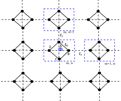
Figure 1: (Color online) The lattice geometry of 2D diamond-octagon lattice is shown. The diamond plaquette, consisting four sites at the vortices $A$, $B$, $C$ and $D$, is depicted by dashed blue boxes that refers to the unit cell. The flux $\phi$ is enclosed by the diamond plaquette. The electrons while intra-cell hopping along the closed loop through the diamond arms $A\to B\to C\to D\to A$ thus acquire a phase and the these hoppings are denoted by $t_{\theta}$. The diagonal hoppings $A\to C$ and $B\to D$, denoted by $\lambda$, do not acquire any phase as they do not enclose a closed loop inside the diamond plaquette. $t_{x}$ and $t_{y}$ respectively denote the horizontal and vertical inter-cell hopping between two adjacent diamond plaquettes.

Using discrete Fourier transform, the momentum space description of the Hamiltonian in Eq. (1) can be read as,

$$\bm{H}=\sum_{\bm{k}}{\Psi}^{\dagger}_{\bm{k}}{\mathcal{H}}_{\bm{k}}(\theta){\Psi}_{\bm{k}},$$ (2)

where ${\Psi}^{\dagger}_{\bm{k}}\equiv\left(\begin{matrix}c^{\dagger}_{k_{x},k_{y},A}&c^{\dagger}_{k_{x},k_{y},B}&c^{\dagger}_{k_{x},k_{y},C}&c^{\dagger}_{k_{x},k_{y},D}\end{matrix}\right)$, and ${\mathcal{H}}_{\bm{k}}(\theta)$ is given by,

$${\mathcal{H}}_{\bm{k}}(\theta)=\left(\begin{matrix}0&t_{\theta}e^{i\theta}&t_{y}e^{ik_{y}}+\lambda&t_{\theta}e^{-i\theta}\\ t_{\theta}e^{-i\theta}&0&t_{\theta}e^{i\theta}&t_{x}e^{ik_{x}}+\lambda\\ t_{y}e^{-ik_{y}}+\lambda&t_{\theta}e^{-i\theta}&0&t_{\theta}e^{i\theta}\\ t_{\theta}e^{i\theta}&t_{x}e^{-ik_{x}}+\lambda&t_{\theta}e^{-i\theta}&0\\ \end{matrix}\right).$$ (3)

We have taken $\epsilon_{i}=0$, $i\in\{A,B,C,D\}$ being the 4 vortices of the diamond plaquette. One can extract all the interesting features about the band structure of the static system as well as driven system as presented in the next section.

Now we shall describe the dynamical scheme. In our present work, we study the effect of a generic aperiodic temporal variation of the flux Hamiltonian ${\mathcal{H}}_{\bm{k}}(\theta)$. We consider the step-like driving protocols with a binary disorder in the amplitude of driving. Interestingly, one can easily recover the periodic limit from the above driving protocol without any loss of generality. We consider two Hamiltonians ${\mathcal{H}}_{\bm{k}}(\theta_{0})$ and ${\mathcal{H}}_{\bm{k}}(\theta_{1})$ in one time-period having magnetic flux $\theta_{0}$ and $\theta_{1}$, respectively. The explicit driving protocol is given by

$${\mathcal{H}}_{\bm{k}}(t) ={\mathcal{H}}_{\bm{k}}(\theta_{0})~{}~{}~{}\quad\text{for}~{}~{}(n-1)T<t<n^{\prime}T,$$ (4)

$$=(1-g_{n}){\mathcal{H}}_{\bm{k}}(\theta_{0})+g_{n}{\mathcal{H}}_{\bm{k}}(\theta_{1})\quad\text{for}~{}~{}n^{\prime}T<t<nT,\quad$$

with $n^{\prime}=n-1+\alpha$. Here, $T$ is the time period, $\alpha$ is a parameter defined between $0$ and $1$ and $n$ refers to the $n$-th stroboscopic period. As a result, the system is evolved by the Hamiltonian $\mathcal{H}_{\bm{k}}(\theta_{0})$ for time duration $\alpha T$, whereas the Hamiltonian $\mathcal{H}_{\bm{k}}(\theta_{1})$ or $\mathcal{H}_{\bm{k}}(\theta_{0})$ can take care the dynamics for the remaining time $(1-\alpha)T$ within one time-period depending on the value of $g_{n}$. The two step Hamiltonians in $k$-space refer to the system on diamond-octagon lattice in real space with two different fluxes $\theta_{0}$ and $\theta_{1}$, respectively. The random variable $g_{n}$ takes the value either $1$ with probability $p$ or $0$ with probability $(1-p)$ chosen from a Binomial distribution. For $g_{n}=0$, the system evolves with the Hamiltonian having flux $\theta_{0}$ in the $n$-th time period within the time interval $(n-1)T$ to $nT$, while $g_{n}=1$ corresponds to the step driving i.e., the subsequent evolution is governed by ${\mathcal{H}}_{\bm{k}}(\theta_{0})$ and ${\mathcal{H}}_{\bm{k}}(\theta_{1})$ for time duration $\alpha T$ and $(1-\alpha)T$, respectively, within a time period.

We note that if initial state is chosen to be the ground state of ${\mathcal{H}}_{\bm{k}}(\theta_{0})$, the case with $g_{n}=0$ refers to the free evolution, whereas, for $g_{n}=1$, the dynamics is non-trivial. Thus the random variable $g_{n}$ introduces aperiodicity in the system. In addition, the parameter $\alpha$ determines time duration of switching between two Hamiltonians ${\mathcal{H}}_{\bm{k}}(\theta_{0})$ and ${\mathcal{H}}_{\bm{k}}(\theta_{1})$, over one time-period in the case of $g_{n}=1$. As a result, for $g_{n}=1$ and $\alpha=0.5$ (i.e., equally divided time duration within a single time-period), the dynamics of the initial state is governed by the product of two unitary matrices (see Eq. (6)) which is designated by Bang-Bang protocol. For $p=1$ i.e., $g_{n}=1$ for all $n$, the problem reduces to periodic one which can be formulated using the Floquet theory. The details are given below.

In general, the initial state $|\Psi_{\bm{k}}(\theta_{\rm ini},0)\rangle$ can be considered as the ground state of the Hamiltonian ${\mathcal{H}}_{\bm{k}}(\theta_{\rm ini},t=0)$ with flux $\theta_{\rm ini}$. One can choose $\theta_{\rm ini}=\theta_{0}$ for simple situation where the dynamics starts from the ground state of the first step Hamiltonian, otherwise, for $\theta_{\rm ini}\neq\theta_{0}$, it is always a non-eigenstate evolution even for $g_{n}=0$. In this way, we have a complete freedom on the choice of initial state for the subsequent dynamics. For the periodic driving in Sec. III.1, we restrict ourselves to the case $\theta_{\rm ini}=\theta_{0}$ while for aperiodic driving in Sec. III.2, $\theta_{\rm ini}\neq\theta_{0}$ and $\theta_{\rm ini}=\theta_{0}$ both the situation are considered. We shall also explore the situation where $\theta_{0}\neq 0$ and $\theta_{0}\neq\theta_{1}$. Throughout this paper we have considered $\hbar=1$. The frequency $\omega$ is the dimension of inverse of time. It enters in the system through the Floquet operator where it appears with the multiplication of energy, and the whole quantity becomes dimensionless (see around Eq. (5)). Similarly, $t_{x}$, $t_{y}$ and $\lambda$ are dimension of energy. We have assumed here $t_{x}$, $t_{y}$ and $\lambda$ to be $1$ such that all the relevant observables are measured in units of these hopping strengths (see Sec. IV for experimental estimations). In this work, we consider the high frequency limit for both periodic and aperiodic drives so that our results are valid well above the resonance limit russomanno12 ; nag14 ; bhattacharya18 . This limit is set by considering the driving frequency greater than the band-width for the equilibrium case and assumed to be $\omega=8$ for all our numerical calculations. We average over $10^{3}$ realization for the aperiodic case.

Coming back to Floquet theory, we here consider a time periodic Hamiltonian $H(T+t)=H(t)$ where $T$ being the time period. In our case, for each ${\bm{k}}$ mode, we then have ${\mathcal{H}}_{{\bm{k}}}(t+T)={\mathcal{H}}_{{\bm{k}}}(t)$. Using the Floquet formalism, one can define a Floquet evolution operator ${\mathcal{F}}_{\bm{k}}(T)={\mathcal{T}}\exp\left(-i\int_{0}^{T}{\mathcal{H}}_{{\bm{k}}}(t)dt\right)$, where ${\mathcal{T}}$ denotes the time ordering operator. One can caste the Floquet operator using quasi-energy $\mu^{(j)}_{\bm{k}}$ and quasi-states $|\Phi^{(j)}_{\bm{k}}(T)\rangle$ ${\mathcal{F}}_{\bm{k}}(T)=\sum_{j}e^{-i\mu^{(j)}_{\bm{k}}T}|\Phi^{(j)}_{\bm{k}}(T)\rangle\langle\Phi^{(j)}_{\bm{k}}(0)|$. The point to note here is that $|\Phi^{(j)}_{\bm{k}}(t+T)\rangle=|\Phi^{(j)}_{\bm{k}}(t)\rangle$ for the time periodic Hamiltonian. Therefore, an arbitrary initial state $|\Psi_{\bm{k}}(t=0)\rangle$ can be decomposed in the Floquet basic: $|\Psi_{\bm{k}}(0)\rangle=\sum_{j}r^{(j)}_{\bm{k}}|\Phi^{(j)}_{\bm{k}}(0)\rangle$, where $r^{(j)}_{\bm{k}}=\langle\Phi^{(j)}_{\bm{k}}(0)|\Psi_{\bm{k}}(0)\rangle$ is the overlap of the Floquet modes and the initial wave-function. Combining the above two relations, we get the time evolved wave-function at $t=nT$

$$|\Psi_{\bm{k}}(nT)\rangle={\mathcal{F}}_{\bm{k}}(nT)|\Psi_{\bm{k}}(0)\rangle=\sum_{j}r^{(j)}_{\bm{k}}e^{-i\mu^{(j)}_{\bm{k}}nT}|\Phi^{(j)}_{\bm{k}}(T)\rangle.$$ (5)

In our case of the periodic step driving with Hamiltonian ${\mathcal{H}}_{\bm{k}}(\theta_{0})$ and ${\mathcal{H}}_{\bm{k}}(\theta_{1})$, ${\mathcal{F}}_{k}$ can be exactly written, in the form of,

$${\mathcal{F}}_{\bm{k}}(T)=\exp(-i{\mathcal{H}}_{\bm{k}}(\theta_{1})(1-\alpha)T)\exp(-i\alpha T{\mathcal{H}}_{\bm{k}}(\theta_{0})).$$ (6)

Turning into the aperiodic case $0<p<1$, there exists a probability of $(1-p)$ to evolve the system with the Hamiltonian ${\mathcal{H}}_{\bm{k}}(\theta_{0})$ in every complete period. We can now express the corresponding evolved state after $n$ complete periods as

$$\lvert\Psi_{\bm{k}}(nT)\rangle=\mathcal{U}_{\bm{k}}(g_{n})\mathcal{U}_{\bm{k}}(g_{n-1}).......\mathcal{U}_{\bm{k}}(g_{2})\mathcal{U}_{\bm{k}}(g_{1})\lvert\Psi_{\bm{k}}(\theta_{\rm ini},0)\rangle$$ (7)

with the generic evolution operator given by,

$$\mathcal{U}_{\bm{k}}(g_{n})=\begin{cases}{\mathcal{F}}_{\bm{k}}(T),&\text{if $g_{n}=1$}.\\ U^{0}_{\bm{k}}(T),&\text{if $g_{n}=0$}.\end{cases}$$ (8)

where $\boldmath{\cal{F}}_{k}(T)$ is the usual Floquet operator as given in Eq. (6). On the other hand, $U^{0}_{\bm{k}}(T)=\exp(-i{\mathcal{H}}_{\bm{k}}(\theta_{0})T)$ is the time evolution operator using the first step Hamiltonian ${\mathcal{H}}_{\bm{k}}(\theta_{0})$.

We shall now compute the instantaneous stroboscopic energy $e_{\bm{k}}(nT)$ following both periodic and aperiodic driving. We note that at the stroboscopic instant $t=nT$, the Hamiltonian ${\mathcal{H}}_{\bm{k}}(\theta_{0},t=nT)$ governs the system; this is the starting Hamiltonian also during the course of dynamics: ${\mathcal{H}}_{\bm{k}}(\theta_{0},t=nT)={\mathcal{H}}_{\bm{k}}(\theta_{0},t=0)$. For periodic driving $e_{\bm{k}}(nT)$ is simply given by $e_{\bm{k}}(nT)=\langle\Psi_{\bm{k}}(nT)|{\mathcal{H}}_{\bm{k}}(\theta_{0},t=0)|\Psi_{\bm{k}}(nT)\rangle$. On the other hand, for aperiodic driving, instantaneous stroboscopic energy becomes

$$e_{\bm{k}}(nT) = \langle\Psi_{\bm{k}}(0)\rvert\mathcal{U}_{\bm{k}}^{\dagger}(g_{1})\mathcal{U}_{\bm{k}}^{\dagger}(g_{2}).......\mathcal{U}_{\bm{k}}^{\dagger}(g_{n-1})\mathcal{U}_{\bm{k}}^{\dagger}(g_{n})$$

$$\times {\mathcal{H}}_{\bm{k}}(\theta_{0},t=0)\mathcal{U}_{\bm{k}}(g_{n})\mathcal{U}_{\bm{k}}(g_{n-1})........\mathcal{U}_{\bm{k}}(g_{2})$$

$$\mathcal{U}_{\bm{k}}(g_{1})\lvert\Psi_{\bm{k}}(0)\rangle$$

Using this, we can calculate the residual energy $W$ (also known as work done and excess energy) in the driven system defined as

$$W(nT)=\frac{1}{L^{2}}\sum_{\bm{k}}(e_{\bm{k}}(nT)-e_{\bm{k}}^{\rm ini}(0)),$$ (10)

where $e_{\bm{k}}^{\rm ini}(0)=\langle\Psi_{\bm{k}}(\theta_{\rm ini},0)|{\mathcal{H}}_{\bm{k}}(\theta_{0},t=0)|\Psi_{\bm{k}}(\theta_{\rm ini},0)\rangle$. Similar to the residual energy at finite time, we can calculate it at infinitely long time when the oscillating terms averages out to zero. For periodic driving the asymptotic limit of excess energy can be written as

$$W(n\to\infty) = \frac{1}{L^{2}}\sum_{{\bm{k}}}\Big{[}\sum_{j=1}^{4}|r_{\bm{k}}^{j}|^{2}\langle\Phi_{\bm{k}}^{j}|{\mathcal{H}}_{\bm{k}}(\theta_{\rm ini},t=0)|\Phi_{\bm{k}}^{j}\rangle$$ (11)

$$- e_{\bm{k}}^{\rm ini}(0)\Big{]}.$$

The cross terms carrying the imaginary “$i$” inside the exponential: $r^{p}_{\bm{k}}(r^{q}_{\bm{k}})^{*}\exp(i\mu^{p}_{\bm{k}}t-i\mu^{q}_{\bm{k}}t)$ with $p\neq q$, do not contribute to the stationary value after momentum summation, as determined by the $|r^{p}_{\bm{k}}|^{2}$, for $n\to\infty$. These time-independent terms would eventually survive to yield the non-equilibrium steady state value of the observables russomanno12 ; nag14 ; bhattacharya18 ; Lazarides14 .

We also calculate flux-current $J_{\theta}$ to study the effect of Floquet driving in the system having FBs. We define the flux-current operator as $\hat{J_{\theta}}=\frac{\partial{\mathcal{H}}_{\bm{k}}(\theta)}{\partial\theta}$, given by

$$\hat{J_{\theta}}=\left(\begin{matrix}0&it_{\theta}e^{i\theta}&0&-it_{\theta}e^{-i\theta}\\ -it_{\theta}e^{-i\theta}&0&it_{\theta}e^{i\theta}&0\\ 0&-it_{\theta}e^{-i\theta}&0&it_{\theta}e^{i\theta}\\ it_{\theta}e^{i\theta}&0&-it_{\theta}e^{-i\theta}&0\\ \end{matrix}\right).$$ (12)

We note that the flux-current represents the intra-loop current within the diamond unit cell; that is why it does not depend on ${\bm{k}}$. Now the current associated with a state $|\Psi_{\bm{k}}\rangle$ is given by the expectation value of the operator at that state: $\langle\hat{J_{\theta}}\rangle=\langle\Psi_{\bm{k}}|\hat{J_{\theta}}|\Psi_{\bm{k}}\rangle$. In a similar spirit, we can define current along $x$ and $y$ directions. However, it can be shown that these current identically vanishes in the ground-state for $\theta_{\rm ini}=0$ referring to the fact that there is no inter-loop current present. On the other hand, $\langle\hat{J_{\theta}}\rangle$ remains finite in the ground-state only when $\theta_{\rm ini}\neq 0$.

We can determine the current of any particular static or Floquet band, and also the total current. The flux current in the stroboscopic time evolved state is given by (using Eq. (5))

$$J_{\theta}(nT)=\frac{1}{L^{2}}\sum_{{\bm{k}}}\sum_{j,j^{\prime}=1}^{4}r_{\bm{k}}^{j}(r_{\bm{k}}^{j^{\prime}})^{*}e^{-i(\mu_{k}^{j}-\mu_{k}^{j^{\prime}})nT}\langle\Phi_{\bm{k}}^{j}|J_{\theta}|\Phi_{\bm{k}}^{j}\rangle.$$ (13)

At asymptotically long time the total $\theta$-current can be expressed as

$$J_{\theta}(n\rightarrow\infty)=\frac{1}{L^{2}}\sum_{{\bm{k}}}\sum_{j=1}^{4}|r_{\bm{k}}^{j}|^{2}\langle\Phi_{\bm{k}}^{j}|J_{\theta}|\Phi_{\bm{k}}^{j}\rangle,$$ (14)

where the oscillating terms of the Eq. (13) will be decayed to zero. The stationary value of flux current is again obtained after summing over the oscillating cross term as done for Eq. 11.

We shall now introduce the definition of flatness of the band and quasi-band which will be applicable for static as well as time-dependent cases, respectively. Usually the flatness is defined by the ratio between band-gap and band-width (see supple for details). Now, in this definition, flatness can be high once the band-gap $\gg$ band-width, even though the band width is significantly large. To overcome this problem, we consider a microscopic definition where we calculate the band-width for all points in the BZ and compare it with the absolute band gap of the effective one-dimensional system (i.e., $\propto(1/L)$ with system size $L$). Therefore, in our alternative definition of flatness, we compare the ratio between the local band-width of $i$-th band $e^{i}_{\bm{k}}-e^{i}_{\bm{k}^{\prime}}$ between ${\bm{k}}=(k_{x},k_{y})$ and ${\bm{k}^{\prime}}$ to the absolute gap with a small number $\eta$. Given the fact that FBs are associated with vanishingly small kinetic energy of the quasi-patricles, we can use the velocity to define the flatness of a given energy band. Now we shall formulate it mathematically in detail using the group velocity. The dispersive nature of the energy can be qualitatively computed using the group velocity for $i$-th band along $x$ and $y$ direction

$${v}^{i,x(y)}_{\bm{k}}=\frac{e^{i}_{\bm{k}}-e^{i}_{\bm{k}^{\prime}(k^{\prime\prime})}}{\Delta}$$ (15)

with ${\bm{k}^{\prime}}=(k_{x}-\Delta k_{x},k_{y})$, ${\bm{k}^{\prime\prime}}=(k_{x},k_{y}-\Delta k_{y})$ and $\Delta=2\pi/L$ is the difference between two subsequent ${\bm{k}}$ points. We can now calculate the quantity for each point ${\bm{k}}$ inside the BZ: ${\mathcal{V}}^{i}_{\bm{k}}=\sqrt{(v^{i,x}_{\bm{k}})^{2}+(v^{i,y}_{\bm{k}})^{2}}$. We define the flatness from the fraction of points in the BZ for which ${\mathcal{V}}^{i}_{\bm{k}}<\eta$, $\eta=0.02$. We discuss about the choice of $\eta$ to calculate the flatness in Sec. II of the supplementary material supple . Let us assume that $l$ is the number of points in the BZ satisfying this criterion, flatness is then given by $l/L^{2}$ such that it is normalized: $F=l/L^{2}$. This criterion means the magnitude of resultant velocity becomes vanishingly small which is essentially reflecting the fact that $i$-th band is considered to be non-dispersive once $e^{i}_{\bm{k}}-e^{i}_{\bm{k}^{\prime}}<(2\pi/L)\eta$ for large $L$.

On the other hand, for periodic Floquet driving, we use quasi-energy $\mu^{(i)}_{\mathbf{k}}$ instead of $e^{i}_{\bm{k}}$ to compute the stroboscopic flatness. Therefore, quasi-energy band can be contemplated as FB if $\mu^{(i)}_{\bm{k}}-\mu^{(i)}_{\bm{k}^{\prime}}<(2\pi/L)\eta$. Now for the case of aperiodic dynamics, flatness has to be described as a function the number of stroboscopic intervals. This dynamical flatness is defined from the instantaneous energy $e_{\bm{k}}(nT)=\langle\Psi_{\bm{k}}(nT)\rvert{\mathcal{H}}_{\bm{k}}(\theta_{0})\lvert\Psi_{\bm{k}}(nT)\rangle$, where $|\Psi_{\bm{k}}(nT)\rangle$ is the time-evolved wavefunction. Similar to definition of static flatness, we here perform the derivative on $e_{\bm{k}}(nT)$ w.r.t. $k_{x}$ and $k_{y}$ to compute $v^{x(y)}_{\bm{k}}(nT)$

$$v^{x(y)}_{\bm{k}}(nT)=\frac{e_{\bm{k}}(nT)-e_{\bm{k}^{\prime}(k^{\prime\prime})}(nT)}{\Delta}$$ (16)

We can now calculate the resultant velocity ${\mathcal{V}}_{\bm{k}}(nT)$ that would measure of the flatness of the time evolved band.

In order to find whether an energy band is topologically non-trivial, one can calculate Chern number $C$ for that band. A topological band is characterized by finite non-zero integer value of $C$ while $C=0$ represents the trivial nature. For the static system it is calculated using the normalized wave function of $n$-th band, $|n({\bm{k}})\rangle$ such that ${\mathcal{H}}_{\bm{k}}|n({\bm{k}})\rangle=E_{n}({\bm{k}})|n({\bm{k}})\rangle$. The Berry curvature of $n$-th band using the standard formula haldane-prl2004 is given by,

$${\bm{\Omega}}_{n}(\bm{k})=-{\rm Im}\sum_{m\neq n}\frac{\langle n({\bm{k}})|\nabla\mathcal{H}_{\bm{k}}|m({\bm{k}})\rangle\times\langle m({\bm{k}})|\nabla\mathcal{H}_{\bm{k}}|n({\bm{k}})\rangle}{(E_{n}({\bm{k}})-E_{m}({\bm{k}}))^{2}}.$$

(17)

Using Eq. (17), one can easily evaluate the value of the Chern number for $n$-th band of the system using the following expression,

$${\color[rgb]{0,0,0}C=\dfrac{1}{2\pi}\int_{BZ}\bm{\Omega}_{n}(\bm{k}).d^{2}{\bm{k}}},$$ (18)

where $BZ$ stands for the first Brillouin zone of the corresponding lattice structure. We note that the Berry curvature is a three component vector ${\bm{\Omega}_{n}}=(\Omega_{n}^{x},\Omega_{n}^{y},\Omega_{n}^{z})$ while Chern number $C$ is a scalar. The area element in two-dimensional momentum space is given by $d^{2}{\bm{k}}=dk_{x}dk_{y}\hat{z}$. The Chern number measures the Berry flux enclosed by the closed surface.

We note that for driven system, the topological characterization is subtle where Chern number can be found to be insufficient to provide the complete topological description rudner13 ; fehske17 ; kitagawa10 ; nathan15 ; fehske18 (see supple for detail). However, we restrict ourselves to Chern number only provided the fact that a quasi-static interpretation can work when the system is driven in the high frequency limit aoki16 . We here explicitly show how the Chern number of a given band for a static system can be generalized to a driven system. In the case of periodic driving, the Berry curvatures of Floquet bands are obtained by replacing $E_{n}(\bm{k})$ and $|n({\bm{k}})\rangle$ with $\mu^{(n)}_{\bm{k}}$ and $|\Phi^{(n)}_{\bm{k}}(T)\rangle$, respectively, while the static Hamiltonian is replaced by the time-independent Floquet Hamiltonian. In order to compute the Chern number numerically, we use the method suggested in Ref.fukui14 with $\mu^{(n)}_{\bm{k}}$ and $|\Phi^{(n)}_{\bm{k}}(T)\rangle$. We reiterate that the complete dynamical description of the topological phase requires much more attention. For example, a dynamic phase with Chern number $C=0$ can host edge states rudner13 ; nag21 . This situation can only appear for driven system and does not have any static analogue. In the high frequency limit, the consecutive Floquet Brillouin Zone in the frequnecy space can be found to be well separated allowing us to adopt Chern number description for a given quasi-energy band.

III Results

III.1 Periodic driving

We first study the flatness $F$ and Chern number $C$ for static Hamiltonian ${\mathcal{H}}_{\bm{k}}(\theta)$ (3) as shown in Fig. 2. The static Hamiltonian contains the magnetic flux term. The flatness $F$ of each static energy band $e_{\bm{k}}^{n=1,4}$ is calculated from the group velocity associated with that energy band. On the other hand, the Chern number $C$ is found from the eigenstates $|\Psi_{\bm{k}}\rangle$ of the static Hamiltonian. The bands can simultaneously exhibit non-trivial topology and high flatness ratio at some specific values of $\theta$. For $n=1$ and $3$, topological FBs appear around $\theta=0$, $\pi$ and $2\pi$ (see Fig. 2(a,c)). While for $n=2$ and $4$, topological FBs arise around $\theta=\pi/2$ and $3\pi/2$ (see Fig. 2(b,d)). Therefore, for most of the values of $\theta$, the system remains non-topological, however, for $\theta=m\pi/6$ with $m=1,5,7$ and $11$, the $n=2$ band becomes almost flat. Similarly, trivial FBs appear for $n=3$ at $\theta=m^{\prime}\pi/3$ with $m^{\prime}=1,2,4$ and $5$. In a nutshell, all the bands in the static model support the topological FBs within a very small window of $\theta$. We also observe that, throughout the whole range of $\theta$, either $(1,3)$-th or $(2,4)$-th energy bands have non-trivial topology. The common feature observed here is that Chern number reverses its sign when the flatness becomes maximum except $\theta=m\pi/6$ and $m^{\prime}\pi/3$ as observed for $n=2$ and $3$, respectively. Our aim is to manipulate this window of $\theta$ for the existence of topological FB along with the reversal of Chern number under Floquet driving. The conventional definition of the flatness is extensively discussed in SI supple .

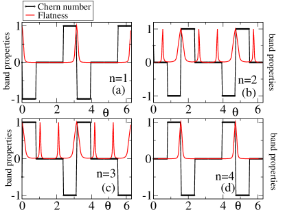
Figure 2: (Color online) Plot depicts the variation of Chern number $C$ and Flatness $F$ as a function of flux $\theta$ for all the energy bands obtained from the static Hamiltonian (3): $n=1$ in (a), $n=2$ in (b), $n=3$ in (c) and $n=4$ in (d). For $n=1,3$, we see that topological flat band is maximally probable around $\theta=0$, $\pi$ and $2\pi$. While for $n=2,4$, one can observe the topological flat band around $\theta=\pi/2$, $3\pi/2$.

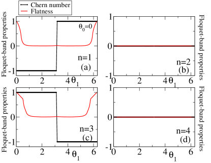
Figure 3: (Color online) Plot depicts the variation of the Chern number $C$ and the flatness $F$ as a function of flux $\theta_{1}$ for all the bands obtained from the Floquet operator Eq. (6): $n=1$ in (a), $n=2$ in (b), $n=3$ in (c) and $n=4$ in (d). For $n=1,3$ only, we see that topological flat band is probable around $0<\theta_{1}<\pi/3$. Here, $\theta_{0}=0$. We note that $\theta_{\rm ini}=\theta_{0}$ and $\alpha=0.8$.

In order to study the effect of Floquet driving on topology and flatness, obtained using quasi-states $|\Phi^{(n)}_{\bm{k}}\rangle$ and quasi-energies $\mu^{(n)}_{\bm{k}}$, we numerically calculate the Chern number and the flatness for the step driving with Hamiltonian ${\mathcal{H}}_{\bm{k}}(\theta_{0})$ and ${\mathcal{H}}_{\bm{k}}(\theta_{1})$ as shown in Fig. 3. We consider here $\theta_{\rm ini}=\theta_{0}=0$. To find the dependence of $\theta_{0}$ on the results, we further repeat our calculation with $\theta_{0}=\pi/3$ as depicted in Fig. 4. From Fig. 3, we observe that the topology and the flatness are completely suppressed for $n=2$ and $n=4$ Floquet bands with $\theta_{0}=0$. As shown in above mentioned figures, in these driving cases, we have another flux parameter $\theta_{1}$ which is tuned to find topology and flatness in quasi-energy bands. We observe that the region of topological flat band with respect to $\theta_{1}$ increases for $n=1$ and $n=3$ Floquet bands as compared to the static case. It is very interesting to note that the value of $\theta_{0}$ is almost same with $\theta_{1}$ around which the expansion of the flatness is observed. The important point to note here is that for $\theta_{0}=\theta_{1}=\pi/3$, $n=3$ Floquet band, obtained from $|\Phi^{(n)}_{\bm{k}}(T)\rangle$, support an extended trivial flat region (see Fig. 4(c)). Unlike to the earlier case with $\theta_{0}=0$, we here find that the flatness and the non-trivial topology can even co-exist for a single Floquet band; $n=2$ band for $\theta_{0}=\pi/3$ becomes nearly flat with $C=-1$ around $\theta_{1}=0.1$ and $1.85$ (see Fig. 4(b)). This reflects the fact that the relationship between the topology and the flatness, associated with odd and even Floquet bands, for $\theta_{0}=0$, is substantially changed for $\theta_{0}=\pi/3$.

Our motivation behind considering two different $\theta_{0}$ is to selectively tune individual bands as topologically flat or trivially flat or topologically dispersive by using another flux parameter $\theta_{1}$. One can obtain the non-topological dispersive bands for $n=2,4$ in the whole regime of $\theta_{1}$ with $\theta_{0}=0$. We want to investigate whether one can generate topology and flatness separately for such bands using other values of $\theta_{0}=\pi/3$. Interestingly, we find that, for $\theta_{0}=\pi/3$, the $n=2$ band can be made topological with $C=-1$ and it shows non-zero flatness values around $\theta_{1}=0$ and $\theta_{1}=1.98$. On the other hand, the $n=3$ band becomes topologically trivial, although it shows non-zero flatness for $0\leq\theta_{1}\leq 2$. Therefore, in general, we can dynamically control topological and flatness properties of a particular band depending on our requirement. We emphasize that once a given band supports topology or flatness or both of them in statics, the Floquet machinery enables us to amplify these initial properties in a desired manner.

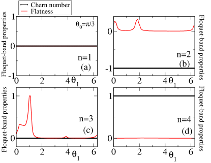
Figure 4: (Color online) We repeat Fig. (3) for $\theta_{0}=\pi/3$. The topological flat band exists here around $\theta_{1}=0.1$ and $1.85$ for the band $n=2$ only.

After investigating topology and flatness of energy and quasi-energy bands numerically for the static and periodic cases, respectively, we now discuss some interesting aspects of corresponding results. One major success of Floquet dynamics is that one can tune the parameters of the system such that it contains topologically non-trivial flat bands. Choosing $\theta_{0}$ in such a way that the corresponding static system has topological FBs, we show that the Floquet technique allows us to successfully enhance the flux domain within which bands can have non-trivial topology and significant flatness compared to the static case. As discussed before, using Floquet dynamics, a particular band can be selectively made trivially flat, topologically dispersive or trivially dispersive. On the other hand, the static system does not support any band that shows non-topological and/or dispersive behavior throughout the whole range of $\theta$. In contrary, Floquet bands can be made trivial and dispersive irrespective of the value of $\theta_{1}$. Therefore, Floquet driving can indeed pave the way towards a better tunability of the bands by incorporating a larger parameter space. We note that our aim is to look for the flatness and topology for each individual quasi-energy band. We are not interested in the topological property of a phase as a whole in the driven system. One can compute $W_{3}$ invariant in order to properly justify a phase with its corresponding boundary edge modes as discussed above rudner13 . In order to obtain a complete understanding of the driven system including its individual quasi-energy bands, $W_{3}$ can be found to be very importanat that we leave for future study (see supple for detail).

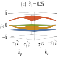
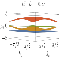
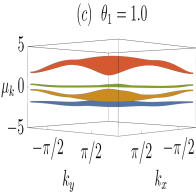
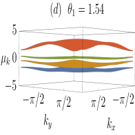
Figure 5: Plot of quasi-energy bands in the ${\bm{k}}$ space for the Floquet operator with the step Hamiltonian having $\theta_{0}=0$ and $\theta_{1}=0.25$ in (a), $0.55$ in (b), $1.0$ in (c) and $1.54$ in (d). It can be observed that the quasi-energy bands $n=1$ and $n=3$ are nearly flat here. Floquet driving can indeed expand the parameter space in terms of $\theta_{1}$ for observing flat bands. Here, frequency of the driving is considered $\omega=8.0$.

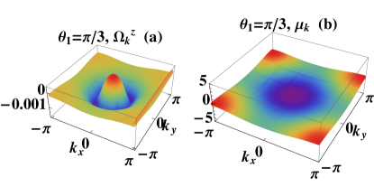
Figure 6: (Color online) The Floquet Berry curvature (left panel) and the corresponding ground state ($n=1$) quasi-energy $\mu^{(1)}_{\bm{k}}$ of the Floquet Hamiltonian (right panel) for $\alpha=0.9$ and $\theta_{1}=\pi/3$. The quasi-energy band is nearly flat as also can be seen from Fig. 7(b). We consider $\theta_{\rm ini}=\theta_{0}=0$.

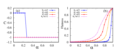
Figure 7: (Color online) (a) The Chern number $C$ of Floquet quasi-energy spectrum for $n=1$ is plotted as a function of $\alpha$ for different values of $\theta_{1}$ with $\theta_{0}=0$. (b) The flatness of the same spectrum as a function of $\alpha$ for the same values of $\theta_{1}$.

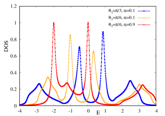
Figure 8: (Color online) The Floquet quasi-energy density of states (DOS) for different values of $\theta_{1}$ and $\alpha$. We consider $\theta_{\rm ini}=\theta_{0}=0$.

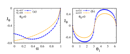
Figure 9: (Color online) (a) The total flux current $J_{\theta}$ as a function of $\alpha$ for two values of $\theta_{1}=\pi/3$ and $\pi/6$ after infinite number of step drives $n\to\infty$. (b) The variation of $J_{\theta}$ with $\theta_{1}$ for $\alpha=0.8$ and $0.9$ at $n\to\infty$. We consider $\theta_{\rm ini}=\theta_{0}=0$.

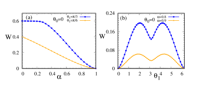
Figure 10: (Color online) (a) Plot of the residual energy $W$ as a function of $\alpha$ for $\theta_{1}=\pi/3$ and $\pi/6$ after infinite number of step drives $n\to\infty$. (b) Here $W$ is plotted as a function of $\theta_{1}$ for $\alpha=0.8$ and $0.9$ at $n\to\infty$.

We now discuss about the Floquet band structures and consider the effect of flux on those. We also show the distribution of Berry curvature in $(k_{x},k_{y})$-plane corresponding $n=1$ band under periodic driving. The static and Floquet band structures have been extensively studied in SI supple . In Fig. 5, we have shown Floquet quasi-energy bands in ${\bm{k}}$-space with $\theta_{0}=0$ and four different values of $\theta_{1}$. It is found that the bands $n=1$ and $n=3$ are perfectly flat for $\theta_{1}=0.25$ as far as their visibilities are concerned. On the other hand, they become nearly flat as $\theta_{1}$ is increased further, but the other two bands become dispersive. We find that the flatness of $n=1$ and $n=3$ bands sustains up to $\theta_{1}=1.0$ (with $\theta_{0}=0$), whereas for the static case these bands can only become flat near $\theta\to 0$. We have already measured the flatness of all the bands for same setting as here (see Fig. 3). We can find that our observations for quasi-energy bands show a good agreement with the measured flatness of respective bands (see Figs. 5 and 3). In Fig. 6, we plot the Berry curvature $\Omega_{n}({\bm{k}})$ and the Floquet energy $\mu^{(n)}_{\bm{k}}$ for $n=1$ with $\theta_{0}=0$ and $\theta_{1}=\pi/3$. We can observe that the quasi-energy band is nearly flat for this case. It is noteworthy that the distribution of Berry curvature complements the behavior of the Floquet band for the above mentioned case.

Having shown the effect of $\theta_{0}$ and $\theta_{1}$ on the FBs, we next want to investigate the effect of duration of the first step Hamiltonian ${\mathcal{H}}_{\bm{k}}(\theta_{0})$ in one complete period $T$ by analyzing $C$ and $F$ as a function of $\alpha$ using Eq. (6). In particular, the Chern number of $n=1$ band is numerically calculated for various values of $\theta_{1}$ (see Fig. 7(a)). We can see that $C$ remains at $-1$ for small values of $\theta_{1}$ such as $\pi/6$, $\pi/9$ and $\pi/12$, during the whole regime of $\alpha$. On the other hand, the important observation is that if we start with a comparatively larger $\theta_{1}$ say, $\theta_{1}=\pi/3$, $C$ remains at $0$ for smaller values of $\alpha$ but it becomes $-1$ at $\alpha\approx 0.24$ and remains there for further increment of $\alpha$. We are now interested to find the topologically non-trivial band which are nearly flat. The flatness of the Floquet band is numerically calculated as a function of $\alpha$ (see Fig. 7(b)) for the same values of $\theta_{1}$ as used to determine the Chern number. One can see here that flatness of the band is increased with increasing $\alpha$, i.e., increasing the duration of $\theta_{0}$ in Floquet evolution.

The flatness remains at larger values as $\theta_{1}$ is decreased throughout the whole regime of $\alpha$. This observation is in congruence to Fig. 3 for small values of $\theta_{1}$. It can be noted that at two extreme values of $\alpha$, i.e., $\alpha=0$ and $1$, the values of $C$ and $F$ are solely determined by ${\mathcal{H}}_{\bm{k}}(\theta_{1})$ and ${\mathcal{H}}_{\bm{k}}(\theta_{0})$, respectively. Therefore, following results at these two extreme values of $\alpha$ are compatible with Fig. 2 for the static case. On the other hand, for $0<\alpha<1$, both the Hamiltonians are responsible to produce the mentioned results. The non-zero Chern number for finite $\alpha(<1)$ is an outcome of the Floquet driving. We therefore find that one can get a better control to selectively manipulate the flatness and topology even by varying $\alpha$ keeping $\theta_{1}$ fixed. The Floquet operator is a function of $\alpha$, $\theta_{1}$, $\theta_{0}$; hence, we are able to achieve a large parameter space for obtaining topological FBs as compared to the static case which is only restricted to $\theta$.

We here examine another approach to detect the FBs using Floquet density of states (FDOS) as $\sum_{{\bm{k}},n}\delta(E-\mu^{(n)}_{\bm{k}})$. However, the topological features of the bands can not be probed using this method. Here we calculate the number of ${\bm{k}}$ points corresponding to a single quasienergy value and plot that number as a function of quasi-energy (see Fig. 8). We find a few peaks in the FDOS for different values of $\theta_{1}$ and $\alpha$ with $\theta_{0}=0$. If we compare FDOS with the flatness as shown in Fig. 7(b), we can make a connection of the behavior of FDOS with the flatness of the quasienergy bands. For $\theta_{1}=\pi/3$ and $\alpha=0.1$, one can find that the quasienergy band ($n=1$) is dispersive in nature (see Fig. 7). The dispersive nature of the band is clearly reflected in the Fig. 8 where we can see that height of the peak around $E=-3$ in the FDOS is much less than the maximum peak height observed at $E=0,~{}-2$ for $\theta_{1}=\pi/6$ and $\alpha=0.9$. For an another case $\theta_{1}=\pi/6$ and $\alpha=0.1$, the quasienergy band is dispersive (see Fig. 7(b)) which is again accompanied by a small broad peak of the DOS around $E=-2.3$ in Fig. 8. On the other hand, for $\theta_{1}=\pi/6$ and $\alpha=0.9$, we see a large sharp peak in the FDOS around $E=-2$ indicating that a FB is supported as the measure of flatness shown in Fig. 7(b). In addition, we observe an identical peak in the FDOS at $E=0$ which is corresponding to $n=3$ FB. This result confirms the fact that the Floquet flat bands appear in pair for $\theta_{0}=0$ (see Fig. 2).

The total flux current (see Eq. (14)) and the residual energy (see Eq. (11)) are also calculated as a function of both $\alpha$ and $\theta_{1}$ at infinitely large time limit as shown in Fig. 9 and Fig. 10, respectively. The total current $J_{\theta}$ is plotted against $\alpha$ for $\theta_{1}=\pi/3$ and $\pi/6$. As $\alpha$ increases the total current approaches to zero from negative values and finally becomes zero at $\alpha=1$. Since all the four bands contribute in calculating total flux current (see Eq. (14)), the negative value of $J_{\theta}$ indicates that the contribution comes mostly from $n=1$ (See supple for detail). The another point to note that, for $\theta_{1}=\pi/3$, $J_{\theta}$ initially decreases and then starts to increase following a minimum value around $\alpha=0.4$. This type of behavior is not observed in the case of $\theta_{1}=\pi/6$, where $J_{\theta}$ is a monotonically increasing function of $\alpha$. We can make a connection of such different behavior of $J_{\theta}$ for $\theta_{1}=\pi/3$ with the Chern number of the $n=1$ band for same $\theta_{1}$. It can be seen that the Chern number for $\theta_{1}=\pi/3$ changes from $0$ to $1$ around $\alpha\approx 0.23$, whereas it stays at $-1$ for other values of $\theta_{1}$ (see Fig. 7(a)). Although the values of $\alpha$ do not exactly match where the changes occur in $J_{\theta}$ and $C$, we can argue that the behavior of $J_{\theta}$ with $\alpha$ has a close connection with the topology of the bands.

The total flux current also shows periodic behavior with $\theta_{1}$ as found in each component of the same current (see supple for detail). The point to note here is that $|J_{\theta}(n\to\infty)|$ acquires higher value as $\alpha$ decreases i.e., the longer the duration of the second step Hamiltonian ${\mathcal{H}}_{\bm{k}}(\theta_{1})$: the flux current of large magnitude is generated in the driven system. Most importantly, the underlying static system, as described by ${\mathcal{H}}_{\bm{k}}(\theta_{\rm ini}=0)$, does not support flux current, the Floquet dynamics allows the system to gain a finite flux current. Similar to each component of the flux current, the total flux current also crosses zero at $\theta_{1}=\pi$ where the sign of Chern number also reverses for $n=1$ and $n=3$ bands (see Fig. 3). Therefore the total flux current can be used as an indicator of change of topology in the system. On the other hand, the residual energy of the system decreases with $\alpha$ and vanishes at $\alpha=1$. We have also seen that the flatness increases with $\alpha$ for any value of $\theta_{1}$. This indicates that the residual energy can be reduced with increasing the flatness in the band. We find that the residual energy for $\theta_{1}=\pi/3$ remains at nearly constant value up to $\alpha\approx 0.23$ and then monotonically decreases with zero value at $\alpha=1$ (see Fig. 10(a)). We have already shown that the Chern number and total flux current exhibit distinct behavior for $\theta_{1}=\pi/3$ as compared to other $\theta_{1}$’s, this also reflects in the behavior of residual energy as a function of $\alpha$. Similar to the flux current, $W$ shows oscillatory behavior as a function of $\theta_{1}$ and the magnitude increases with decreasing $\alpha$, as expected. The excess energy can be minimized for $\theta_{1}=\pi$. From analysis of different observables as a function of $\alpha$ and $\theta_{1}$, we can convey that our work has experimentally viable, as both of the above parameter can be tuned.

We below summarize the main finding of this section. The Floquet FBs (see Fig. 3 and Fig. 4) can be generated and detected using FDOS (see Fig. 8). The static flatness and topology (see Fig. 2) can thus be tuned with driving parameters $\theta_{0}$, $\theta_{1}$ and $\alpha$. The demonstration of Floquet quasi-bands are shown explicitely in Fig. 5. The structure of Berry curvature and the topological nature for a given quasi-energy band are shown in Fig. 6 and Fig. 7, respectively. The evolution of driving induced flux current $J_{\theta}$ and excess energy $W$ with $\theta_{1}$ and $\alpha$ are shown in Fig. 9 and Fig. 10, respectively. The parameters i.e., duration of the flux Hamiltonian $H(\theta_{1})$ and the associated flux $\theta_{1}$, yield a better control such as, determining the maxima, minima of the above quantities.

III.2 Aperiodic driving

After studying the flatness, Chern number, flux current and excess energy in periodic Floquet dynamics, we shall now investigate the aperiodic case where $P$ denotes the probability of appearing the second flux Hamiltonian in the driving protocol as defined in Eq. (4). We shall first study the dynamics of excess energy $W$, as obtained from Eq. (LABEL:eq_rs1) and Eq. (10), by varying $\theta_{1}$ and $\alpha$. Figure 11 shows that for $\theta_{1}=\pi/2$ and $\theta_{\rm ini}=\theta_{0}=0$, $W$ increases less rapidly for $\alpha=0.8$. A close observation of the numerical results for different $\alpha$ indicates that $W$ stays at maximum value as a function of time for $P=0.5$, compared to any $P\neq 0.5$ for $\alpha>0.2$. This implies the fact that the system absorbs energy maximally when the degree of aperiodicity is maximum, while for fully periodic drive $P=1$, the system attains a periodic steady state i.e., it does not absorb energy from the external drive. Interestingly, any amount of aperiodicity can drive the system away from the periodic steady state and hence it gets heated up with time. While investigating with $\alpha$, for a given value of $n<300$, we find that short duration of flux-Hamiltonian (i.e., $\alpha=0.8$) can lead to the decrement of $W$ as compared to the long duration of flux Hamiltonian (i.e., $\alpha=0.2$). The finite time rate of growth of $W$ becomes higher for $\alpha=0.2$ while the intermediate rate of growth becomes higher for $\alpha=0.8$. As a result, the asymptotic value of $W$ is reached early for $\alpha=0.2$ while the $W$ saturates for much higher value of $n$ for $\alpha=0.8$. We note that the asymptotic value depends on $\alpha$. The reason behind the above characteristic will be discussed below. The point to note here is that the heating in the system gets remarkably suppressed as we reduce the value of $\theta_{1}$ for any $\alpha$ (See supple for detail).

We would now try to understand the physical picture behind the rise of $W$ and its subsequent saturation at $n\to\infty$. It has been shown for a two level model (in the momentum space) that aperiodic dynamics can be analytically handled in a non-perturbative way bhattacharya18 ; maity18 ; the instantaneous energy $e_{\bm{k}}(nT)$ as defined in Eq. (LABEL:eq_rs1) is proportional to $(D_{\bm{k}})^{n}$ while the proportionality factor depends on initial state $|\Psi_{\bm{k}}(\theta_{\rm ini},t=0)\rangle$ and possible combinations of Floquet basis. The disorder matrix $D_{\bm{k}}$ depends on $P$, $T$, Floquet operator ${\mathcal{F}}_{\bm{k}}$ and eigen-energies of ${\mathcal{H}}_{\bm{k}}(\theta_{0})$. For two level system with binary disorder ($g_{n}$ can be either $1$ or $0$), $4\times 4$ disorder matrix has two real (unity and less than unity) and two complex conjugate (magnitude less than unity) eigenvalues. Now for small $n$, the complex eigenvalues dictate the oscillatory pattern on the overall increasing background. The increasing nature, persisted until $n$ becomes substantially large, is dictated by the real eigenvalue which is less than unity . The asymptotic universal nature is solely determined by the unity eigenvalue as all the other contributions coming from the remaining eigenvalues vanish. Therefore, it is understood that $W$ can not be raised indefinitely rather than it saturates as $n\to\infty$. These saturation values depend on the proportionality factors. Now connecting it to our case, one can similarly construct a $8\times 8$ disorder matrix $D_{\bm{k}}$ as our momentum space Hamiltonian is $4\times 4$. We will be having unity eigenvalue in $D_{\bm{k}}$ that determines the asymptotic results at $n\to\infty$. All the remaining eigenvalues dictates the low and intermediate growth of $W$.

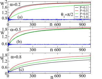
Figure 11: Plot depicts the variation of excess energy $W$ as a function of stroboscopic instant $n$ for $\alpha=0.2$ (a), $\alpha=0.5$ (b), $\alpha=0.8$ (c) with $\theta_{1}=\pi/2$. For the fully periodic situation ($P=1$), the system synchronizes with the external driving and stops absorbing energy. On the contrary, for any non-zero value of P ($\neq 1$), the periodic steady state gets destabilized and the system keeps on absorbing heat. For $P=0.5$, $W$ grows maximally with $n$ almost independent of the values of $\alpha$. We note that with increasing $\alpha$, the rate of growth of $W$ as a function of $n$ increases. Here, we have $\theta_{\rm ini}=\theta_{0}=0$.

Turning to periodic dynamics with $P=1$, we observe by analyzing Fig. 11 that the system attains periodic steady state with minimum excess energy when the flux Hamiltonian is activated for short duration of time within one time-period and flux $\theta_{1}\to 0$. Both of the above observations are associated with the fact that the initial state is the ground state of Hamiltonian with $\theta_{0}=0$. For aperiodic case, we also note that the asymptotic value of $W$ at $n\to\infty$ is a function of $\theta_{1}$ and $\alpha$.

We shall now study the dynamical flatness by varying different parameters such as $\theta_{1}$, $\alpha$ and $P$. We show that for $\theta_{1}\gg 0$, the time evolved instantaneous energy becomes highly dispersive irrespective of the duration $\alpha T$ of the no-flux Hamiltonian. This has been quantified by calculating $F$ using Eq. (16) and shown in Fig. 12. The time evolved $e_{\bm{k}}(nT)$ can have non-dispersive nature as far as small $n$ is concerned. The aperiodic driving leads to significant flatness as compared to the periodic driving for small but finite $n$ limit. This scenario is clearly visible for small $\theta_{1}$, say $\theta_{1}=\pi/40$, irrespective of the duration of the no-flux Hamiltonian (see Fig. 12) We find that for periodic driving with $P=1$, $e_{\bm{k}}(nT)$ becomes less dispersive if one increases the duration of no-flux Hamiltonian from $\alpha=0.2$ to $0.8$. We see that $F$ remains at closely unit value for $P=0.1$ with $\alpha=0.8$, while flatness falls most rapidly for $P=1$ as far as $n\leq 200$. This is due to the fact that the time-evolved wavefunction $\lvert\Psi_{\bm{k}}(nT)\rangle$ is minimally deviated from the initial wave-function for $P=0.1$ and $\alpha=0.8$, i.e., the system is closely following trivial evolution as the flux-Hamiltonian is mostly inactive and its duration is very short over a time-period. At the same time, we know that the initial no-flux Hamiltonian supports non-topological flat band as the ground state. Hence, for such aperiodic driving, the flatness remains nearly constant at unity for small time and then starts decaying since flux-Hamiltonian even for short duration is effectively active at large time. On the other hand, for periodic case with $P=1$, due to the similar reason the fluctuation of $F$ gets reduced heavily when $\theta_{1}\to 0$ and $\alpha\to 1$. The flatness of the instantaneous state $|\Psi(t=nT)\rangle$ is closely connected to the the survival probability of an initial state $P_{s}=|\langle\Psi(t=0,\theta_{\rm ini})|\Psi(t=nT)\rangle|^{2}$. From the behavior of instantaneous flatness it can be estimated that $P_{s}$ decays with $n$, however, there always exists a finite $P_{s}$ even for large $n$ (See supple for detail).

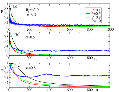
Figure 12: Plot depicts the variation of instantaneous flatness $F$ as a function of stroboscopic instant $n$ for $\alpha=0.2$ (a), $\alpha=0.5$ (b), $\alpha=0.8$ (c) with $\theta_{1}=\pi/40$. One can see that periodic and aperiodic driving both are not able to generate flat band. We here choose $\theta_{\rm ini}=\theta_{0}=0$. The instantaneous flatness acquires higher values for periodic dynamics. We here choose $\theta_{\rm ini}=\theta_{0}=0$.

Until now we have considered the situations with $\theta_{\rm ini}=\theta_{0}$, we will now investigate the case where $\theta_{\rm ini}\neq\theta_{0}$ i.e., initial state is not the eigenstate of the first step Hamiltonian ${\mathcal{H}}_{\bm{k}}(\theta_{\rm ini})$. Considering two different $\theta_{\rm ini}$ and keeping $\theta_{1}$, $\theta_{0}$ fixed, we will be able to compare the two equivalent non-eigenstate evolution as far as the first step Hamiltonian ${\mathcal{H}}_{\bm{k}}(\theta_{0})$ is concerned. Using this method, we can analyze the effect of initial flat as well as dispersive bands on $W$ following the identical dynamical protocol. We investigate the residual or excess energy $W$ as a function of $n$ considering different initial states and a variety of step Hamiltonians for the periodic and aperiodic driving as shown in Fig. (13), Fig. (14). The interesting outcome is that in the case of aperiodic driving the growth rate of $W$ becomes heavily slowed down if the initial state has a significant flatness.

We study the evolution of excess work $W$ for $\theta_{1}=\pi/2$ and $\pi/6$ with $P=1$ and $0.5$ as shown in Fig. 13(a) and (b), respectively. The excess energy $W$ turns out to be negative for the periodic driving and also for the aperiodic driving for small time; this is due to the fact that instantaneous energy $e_{\bm{k}}(nT)$ is less than the initial energy $e^{\rm ini}_{\bm{k}}(0)$ (see Eq. (10)). In the present case, $e^{\rm ini}_{\bm{k}}(0)$ is not an eigenstate energy. One can observe that the periodic driving is not able to excite the system. However, aperiodic driving can not lead to a periodic steady state and hence, instantaneous energy $e_{\bm{k}}(nT)$ can overcome $e^{\rm ini}_{\bm{k}}(0)$. Most interestingly, the growth rate of $W$ is significantly suppressed once the initial state has substantial flatness; the energy eigenvalues corresponding to the state $|\Psi_{\bm{k}}(\theta_{\rm ini},t=0)\rangle$ are more flat for $\theta_{\rm ini}=\pi$ as compared to $\pi/2$. In order to examine these features in detail, we repeat the aperiodic case with $P=0.5$ as depicted in Fig. 14(a) for $\theta_{1}=\pi/2$. One can clearly observe that $W$ calculated from initial dispersive band saturates at a higher value compared to the initial FB. On the other hand, for the periodic case, the behavior is the opposite (see Fig. 14(b)); $W$ obtained from an initial dispersive band saturates at a smaller value as compared to an initial FB. The reason is $e^{\rm ini}_{\bm{k}}(0)$ for dispersive band becomes lower compared to the FB. This behavior as expected does not change for aperiodic dynamics. Since the system does not keep absorbing energy from the periodic driving, $W$ for dispersive band always stays lower compared to that of the FB.

We can clearly observe that the initial flatness of a band has a significant effect on the subsequent dynamics. For the aperiodic case, as we know that the disorder matrix $D_{\bm{k}}$ does not depend on initial condition, rather it is the proportionality factor that depends on the initial condition. In the present analysis by keeping the two step flux Hamiltonians fixed, we consider different situations by varying initial conditions. Therefore, we actually change the proportionality factor instead of changing the disorder matrix. One can find that both the instantaneous energies $e(\theta_{\rm ini}=3.05,~{}3.0,t=nT)$ and $e(\theta_{\rm ini}=1.0,~{}2.0,t=nT)$ saturate to an identical value irrespective of the initial flatness as observed in terms of the survival probability $P_{s}$ (see Sec. VII of the Ref. supple for more detail). The instantaneous energy rises more with time and eventually leading to a longer saturation time while starting from an initial FB rather than a non-flat band. This may be the reason to saturate the excess energy $W$ to a higher positive value when the initial state is substantially flat. This initial state dependence is further confirmed by varying the dynamical parameter $P$ and $\theta_{1}$ while keeping $\theta_{\rm ini}$ fixed (see Fig. 14). Moreover, the small time rise of $W$ is almost identical for the different $\theta_{\rm ini}$ as discussed above. Similar to the asymptotic value, the intermediate growth rate of $W$ increases for initial dispersive band as compared to the FBs.

We below provide a plausible argument behind above oberservation. The high degeneracy of the initial FB can act as an energy absorbing agent while the system is driven out of equilibrium. The excited quasi-particle due to driving can not fill the states above until they occupy all the degenerate states of the FBs. The quasi-particles associated with a flat band have the same energy. To excite those at the higher level, each quasi-particle needs same amount of energy from the driving. As a result, system needs a large amount of energy to excite all the quasi-particles. In comparison, the initial dispersive band hosts non-degenerate quasi-particles that are easily excited by absorbing energy from driving. As a result, the subsequent dynamics starting from initial FB and dispersive band are quite different.

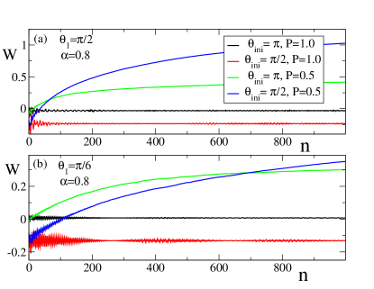
Figure 13: Plot depicts the variation of instantaneous work with stroboscopic cycle $n$ with two step Hamiltonian ${\mathcal{H}}_{\bm{k}}(\theta_{0}=0)$ and ${\mathcal{H}}_{\bm{k}}(\theta_{1}=\pi/2)$ considering the ground state of ${\mathcal{H}}_{\bm{k}}(\theta_{\rm ini})$ as initial state $|\Psi_{\bm{k}}(\theta_{\rm ini,t=0})\rangle$. (a) for $\theta_{1}=\pi/2$ and (b) for $\theta_{1}=\pi/6$. We find for the aperiodic driving with $P=0.5$, $W$ increases more rapidly once we start from dispersive band at $\theta_{\rm ini}=\pi/2$ compared to a FB at $\theta_{\rm ini}=\pi$. However, for periodic driving $P=1$, $W$ saturates at higher value starting from dispersive band compared to FB. Here, $\alpha=0.8$.

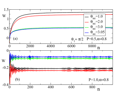
Figure 14: Plot depicts the variation of instantaneous work done as a function of stroboscopic cycle $n$ for aperiodic $P=0.5$ (a) and periodic $P=1.0$ (b) driving with $\theta_{1}=\pi/2$. Starting from a FB ($\theta_{\rm ini}=3.0,~{}3.05$), $W$ saturates to a lower value as compared to dispersive band ($\theta_{\rm ini}=1.0,~{}2.0$). Here, $\alpha=0.8$.

We demonstrate the evolution of excess energy and instantaneous flatness in Fig. 11 and Fig. 12, respectively. We here find that aperiodic (periodic) driving leads to heating (non-equilibrium steady state without heating) and consequently a substantial dispersiveness is generated in the time evolved state. Now the heating can be reduced while we start from an initial flat band rather than dispersive band as shown in Fig. 13. We next verify this finding by considering different combination of initial states and Floquet operators as shown in Fig. 14.

IV Experimental feasibility

From previous literatures on the flat bands, we know that they arise due to the destructive quantum phase interference of fermion hopping paths in tight-binding systems on different lattices. There could be two possible experimental techniques to fabricate such lattice structure in laboratory; one is photonic waveguide and the other is optical lattice. The aberration-corrected femtosecond laser-writing method can efficiently yield a precise fabrication of two-dimensional arrays of sufficiently deep single-mode waveguides. The two-dimensional Lieb lattice structure Vicencio15 ; Mukherjee15 and other lattice geometries Longhi14 ; Zong16 are successfully realized using photonic waveguides. The diamond-octagon lattice structure can also be realized experimentally using photonic waveguide with the values of the experimental parameters as: the lattice period $20-30$  $\mu$m, propagation distance $7-10$ cm, and operating wavelength $500-800$ nm Vicencio15 ; Mukherjee15_2 . The topological properties of a lattice structure can also be investigated experimentally using optical waveguide Zhong19 . On the other hand, ultracold atomic condensates in optical lattices can artificially generate lattice structure by suitably tuning the hopping amplitudes, interaction strength and potential depth bloch-rmp2008 . The tunable effective magnetic field can be generated for ultracold atoms in optical lattices Aidelsburger11 . Similarly, we can realize our model in the laboratory using ultracold atoms in optical lattice. To observe our results, the frequency of the step driving has to be large as compared to the band-width of the system and the magnetic field has to be comparable with the square of the lattice spacing such that $\theta$ becomes finite $[0,2\pi]$. As far as the numerical values of the experimental parameters are concerned, we estimate those as, switching frequency $\omega\sim 1-100$ ev with $t_{x},~{}t_{y},~{}\lambda\sim 0.1-10$ ev such that $\omega>t_{x},~{}t_{y},~{}\lambda$, switching time $T\sim 0.01-1.0$ fs and the magnetic field $B\sim 0.1-10.0$ nT. Moreover, in addition to the optical lattice platform we hope that our result can be tested in various metamaterials such as photonic exp1 ; exp2 ; exp3 , acoustic exp4 ; exp5 lattices and solid state systems exp6 .

V Conclusion

Motivated by the recent equilibrium studies on topological FBs Pal18 , we here investigate a two dimensional diamond-octagon model with time dependent flux Hamiltonian. To be precise, the driving protocol considered here is periodic and each cycle is comprised of two step Hamiltonians corresponding to two different magnetic fluxes $\theta_{0}$ and $\theta_{1}$ embedded in them. This Floquet set up allows us to characterize the driven model in terms of the two parameters, 1) duration of first flux Hamiltonian $\alpha T$ and 2) values of flux $\theta_{i}$. Most interestingly, we show that the topological FBs can be engineered quite desirably by appropriately tuning these above parameters for which the static model does not support topology and FB simultaneously. In the process, we provide a new definition of flatness and check the consistency of our definition using Floquet density of states (FDOS) where we find sharp peak at the FB energy. We calculate Chern number $C$ and flatness of the Floquet quasi-energy bands by varying $\alpha$ and $\theta_{1}$ to get Floquet topological flat bands. We also show the emergence of flux current corresponding to each Floquet band and describe how this is connected to change of topology in the system. Considering the asymptotic limit of the number of driving cycle $n\to\infty$, we additionally study the total flux current $J_{\theta}$ and the variation of excess energy $W$ as a function of $\alpha$ and $\theta_{i}$. Interestingly, $J_{\theta}$ and $W$ both show periodic behavior with $\theta_{1}$. We also show the interconnections between topology of the bands, flux current, flatness and excess energy of the driven system. Importantly, we show that the excess energy due to periodic drive in the system can be reduced by increasing the initial flatness of the energy bands.

We next analyze the stroboscopic evolution of $W$ and flatness with $n$ considering aperiodic driving. Here the protocol we follow is that the second Hamiltonian inside the cycle is associated with a binary disorder amplitude with probability $P$. In this way, we can go to perfect periodic limit for probability $P=1$ and, $P=0$ corresponds to a situation where the system is evolved only with the first Hamiltonian. Any intermediate value of $P$ corresponds to a random array of these two Hamiltonian. We show that $W$ can be substantially suppressed if $\alpha\to 1$ and $\theta_{1}\to 0$. On the other hand, maximum heating occurs when $\alpha\to 0$ and $\theta_{1}\to\pi/2$. For periodic case, $W$ saturates to a higher value for $\alpha\to 0$ and $\theta_{1}\to\pi/2$ compared to $\alpha\to 1$ and $\theta_{1}\to 0$. We also study the instantaneous flatness that can only sustain with periodic dynamics. Most interestingly, starting from an initial FB, $W$ saturates at a lower value for the aperiodic case; a large number of degenerate states associated with the FBs are responsible for this suppression. We further explain our observation by making resort to the disorder matrix representation of the work done.

In the case of aperiodic driving, we mainly ask the questions that how we can minimize or suppress heating in the system. In experiments, realizing a purely periodic drive is a very difficult task. Therefore, aperiodic drive is more realistic case than the periodic one. On the other hand, heating is a real problem in such cases to realize interesting Floquet phases such as Floquet topological flat bands in the present set up. Interestingly, we show that the heating can be suppressed by reducing the value of flux parameter $\theta_{1}$ in the case of aperiodic driving. Further it can be minimized by choosing appropriate initial state that supports non-dispersive Floquet bands. In this context, our work seems to be useful for its practical implications.

Interestingly, the effect of interactions for systems with flat bands, showing high density of states, is an active area of research wu-prl2007 ; wang13 . The interaction mediated strongly correlated phenomenon such as, superconductivity and fractional quantum Hall effect, thus can come into play when the degeneracy is lifted by the interaction in these systems. It would be indeed interesting to come up with a more realistic model considering the electron-electron Hubbard interaction as the future study. At the same time, delocalization-localization transitions for many-body systems receive enormous attention lazarides15 . Ours study on dynamics of excess energy can be further extended for interacting system that is beyond the scope of the present study. Being focused on the non-interacting systems, one possible future direction could be to explore the dynamic winding number $W_{3}$ invariant extensively for the flat bands while the present study is only limited to Chern number.

References

- (1) K. Sun, Z. Gu, H. Katsura, and S. Das Sarma, Phys. Rev. Lett. 106, 236803 (2011).
- (2) E. Tang, J.-W. Mei, and X.-G. Wen, Phys. Rev. Lett. 106, 236802 (2011).
- (3) T. Neupert, L. Santos, C. Chamon, and C. Mudry, Phys. Rev. Lett. 106, 236804 (2011).
- (4) A. G. Grushin, J. Motruk, M. P. Zaletel, and F. Pollmann, Phys. Rev. B 91, 035136 (2015).
- (5) D. Leykam, S. Flach, O. Bahat-Treidel, and A. S. Desyatnikov, Phys. Rev. B 88, 224203 (2013).
- (6) S. Flach, D. Leykam, J. D. Bodyfelt, P. Matthies, and A. S. Desyatnikov, Europhys. Lett. 105, 30001 (2014).
- (7) J. D. Bodyfelt, D. Leykam, C. Danieli, X. Yu, and S. Flach, Phys. Rev. Lett. 113, 236403 (2014).
- (8) C. Danieli, J. D. Bodyfelt, and S. Flach, Phys. Rev. B 91, 235134 (2015).
- (9) R. Khomeriki and S. Flach, Phys. Rev. Lett. 116, 245301 (2016).
- (10) W. Maimaiti, A. Andreanov, H. C. Park, O. Gendelman, and S. Flach, Phys. Rev. B 95, 115135 (2017).
- (11) S. Rojas-Rojas, L. Morales-Inostroza, R. A. Vicencio, and A. Delgado, Phys. Rev. A 96, 043803 (2017).
- (12) E. Travkin, F. Diebel, and C. Denza, Appl. Phys. Lett. 111, 011104 (2017).
- (13) A. Ramachandran, A. Andreanov, and S. Flach, Phys. Rev. B 96, 161104(R) (2017).
- (14) A. R. Kolovsky, A. Ramachandran, and S. Flach Phys. Rev. B 97, 045120 (2018).
- (15) B. Pal and K. Saha, Phys. Rev. B 97, 195101 (2018).
- (16) K. v. Klitzing, G. Dorda, and M. Pepper, Phys. Rev. Lett. 45, 494 (1980).
- (17) R. B. Laughlin, Phys. Rev. Lett. 50, 1395 (1983).
- (18) H. Tasaki, Phys. Rev. Lett. 69, 1608 (1992).
- (19) A. Tanaka and H. Ueda, Phys. Rev. Lett. 90, 067204 (2003).
- (20) B. Roy, F. F. Assaad, and I. F. Herbut, Phys. Rev. X 4, 021042 (2014).
- (21) V. J. Kauppila, F. Aikebaier, and T. T. Heikkilä, Phys. Rev. B 93, 214505 (2016).
- (22) S. Peotta and P. Törmä, Nat. Comm. 6, 8944 (2015).
- (23) M. Goda, S. Nishino, and H. Matsuda, Phys. Rev. Lett. 96, 126401 (2006).
- (24) J. T. Chalker, T. S. Pickles, and P. Shukla, Phys. Rev. B 82, 104209 (2010).
- (25) D. Guzmán-Silva, C. Mejía-Cortés, M. A. Bandres, M. C. Rechtsman, S. Weimann, S. Nolte, M. Segev, A. Szameit, and R. A. Vicencio, New J. Phys. 16, 063061 (2014).
- (26) R. A. Vicencio, C. Cantillano, L. Morales-Inostroza, B. Real, C. Mejía-Cortés, S. Weimann, A. Szameit, and M. I. Molina, Phys. Rev. Lett. 114, 245503 (2015).
- (27) S. Mukherjee, A. Spracklen, D. Choudhury, N. Goldman, P. Öhberg, E. Andersson, and R. R. Thomson, Phys. Rev. Lett. 114, 245504 (2015).
- (28) S. Mukherjee and R. R. Thomson, Opt. Lett. 40, 5443 (2015).
- (29) S. Longhi, Opt. Lett. 39, 5892 (2014).
- (30) S. Xia, Y. Hu., D. Song, Y. Zong, L. Tang, and Z. Chen, Opt. Lett. 41, 1435 (2016).
- (31) Y. Zong, S. Xia, L. Tang, D. Song, Y. Hu, Y. Pei, J. Su, Y. Li, and Z. Chen, Opt. Express 24, 8877 (2016).
- (32) S. Weimann, L. Morales-Inostroza, B. Real, C. Cantillano, A. Szameit, and R. A. Vicencio, Opt. Lett. 41, 2414 (2016).
- (33) N. Masumoto, N. Y. Kim, T. Byrnes, K. Kusudo, A. Löffler, S. Höfling, A. Forchel, and Y. Yamamoto, New J. Phys. 14, 065002 (2012).
- (34) F. Baboux, L. Ge, T. Jacqmin, M. Biondi, E. Galopin, A. Lemaître, L. L. Gratiet, I. Sagnes, S. Schmidt, H. E. Türeci, A. Amo, and J. Bloch, Phys. Rev. Lett. 116, 066402 (2016).
- (35) G.-B. Jo, J. Guzman, C. K. Thomas, P. Hosur, A. Vishwanath, and D. M. Stamper-Kurn, Phys. Rev. Lett. 108, 045305 (2012).
- (36) S. Taie, H. Ozawa, T. Ichinose, T. Nishio, S. Nakajima, and Y. Takahashi, Sci. Adv. 1, e1500854 (2015).
- (37) V. Apaja, M. Hyrkäs, and M. Manninen, Phys. Rev. A 82, 041402(R) (2010).
- (38) N. Goldman, D. F. Urban, and D. Bercioux, Phys. Rev. A 83, 063601 (2011).
- (39) S. D. Huber and E. Altman, Phys. Rev. B 82, 184502 (2010).
- (40) C. Wu, D. Bergman, L. Balents, and S. Das Sarma, Phys. Rev. Lett. 99, 070401 (2007).
- (41) M. Aidelsburger, M. Lohse, C. Schweizer, M. Atala, J. T. Barreiro, S. Nascimbéne, N. R. Cooper, I. Bloch, and N. Goldman, Nat. Phys. 11, 162 (2015).
- (42) G. Montambaux, L. K. Lim, J. N. Fuchs, and F. Piechon, Phys. Rev. Lett. 121, 256402 (2018).
- (43) W. Jiang, M. Kang, H. Huang, H. Xu, T. Low, and F. Liu, Phys. Rev. B 99, 125131 (2019).
- (44) L. K. Lim, J. N. Fuchs, F. Piéchon, and G. Montambaux, Phys. Rev. B 101, 045131 (2020).
- (45) E. Tang, J. W. Mei, and X. G. Wen, Phys. Rev. Lett. 106, 236802 (2011).
- (46) M. Koshino, N. F. Q. Yuan, T. Koretsune, M. Ochi, K. Kuroki, and L. Fu, Phys. Rev. X 8, 031087 (2018).
- (47) L. Xian, D. M. Kennes, N. Tancogne-Dejean, M. Altarelli, A. Rubio, Nano Lett. 2019, 19, 8, 4934.
- (48) L. Klebl, C. Honerkamp, Phys. Rev. B 100, 155145 (2019).
- (49) L. Balents, C. R. Dean, D. K. Efetov, Dmitri and A.F. Young, Nature Physics, 16, 725 (2020).
- (50) Y. Kuno, T. Orito, and I. Ichinose, New J. Phys. 22, 013032 (2020).
- (51) R. Bistritzer and A. H. MacDonald, PNAS (2011) 108 12233.
- (52) F. Haddadi, Q-S Wu, A. J. Kruchkov, O. V. Yazyev, Nano Lett. 2020, 20, 2410.
- (53) P. Calabrese, and J. Cardy, Phys. Rev. Lett. 96, 136801 (2006); J. Stat. Mech, P06008 (2007).
- (54) M. Rigol, V. Dunjko and M. Olshanii, Nature 452, 854 (2008).
- (55) T Oka, H Aoki, Phys. Rev. B 79 081406 (2009).
- (56) T. Kitagawa, E. Berg, M. Rudner, and E. Demler, Phys. Rev. B 82, 235114 (2010).
- (57) N. H. Lindner, G. Refael and V. Galitski, Nat. Phys. 7, 490-495, (2011).
- (58) A. Bermudez, D. Patane, L. Amico, M. A. Martin-Delgado, Phys. Rev. Lett. 102, 135702, (2009).
- (59) A. A. Patel, S. Sharma, A. Dutta, Eur. Phys. Jour. B 86, 367 (2013); A. Rajak and A. Dutta, Phys. Rev. E 89, 042125, 2014. P. D. Sacramento, Phys. Rev. E 90 032138, (2014); M. D. Caio, N. R. Cooper and M. J. Bhaseen, Phys. Rev. Lett. 115, 236403 (2015).
- (60) M. Thakurathi, A. A. Patel, D. Sen, and A. Dutta, Phys. Rev. B 88, 155133 (2013).
- (61) A Pal and D. A. Huse, Phys. Rev. B 82, 174411 (2010).
- (62) R. Nandkishore, D. A. Huse, Annual Review of Condensed Matter Physics, 6, 15-38 (2015).
- (63) M. Heyl, A. Polkovnikov, and S. Kehrein, Phys. Rev. Lett., 110, 135704 (2013).
- (64) J. C. Budich and M. Heyl, Phys. Rev. B 93, 085416 (2016).
- (65) S. Sharma, U. Divakaran, A. Polkovnikov and A. Dutta, Phys. Rev. B 93, 144306 (2016).
- (66) I. Bloch, J. Dalibard, and W. Zwerger, Rev. Mod. Phys. 80, 885 (2008).
- (67) M. Lewenstein, A. Sanpera, and V. Ahufinger, (Oxford University Press, Oxford (2012)).
- (68) G. Jotzu, M. Messer, R. Desbuquois, M. Lebrat, T. Uehlinger, D. Greif and T. Esslinger, Nature 515, 237 (2014).
- (69) M. Greiner , O. Mandel, T. W. Hansch and I. Bloch, Nature 419, 51 (2002).
- (70) T. Kinoshita, T. Wenger and D. S. Weiss, Nature 440, 900 (2006).
- (71) M. Gring, M. Kuhnert, T. Langen, T. Kitagawa, B. Rauer, M. Schreitl, I. Mazets1, D. Adu Smith, E. Demler, and J. Schmiedmayer, Science 337, 1318 (2012).
- (72) M. Cheneau, P. Barmettler, D. Poletti, M. Endres, P. Schauss, T. Fukuhara, C. Gross, I. Bloch, C. Kollath and S. Kuhr, Nature 481, 484 (2012).
- (73) D. Fausti, R. I. Tobey, , N. Dean, S. Kaiser, A. Dienst, M. C. Hoffmann, S. Pyon, T. Takayama, H. Takagi,4, A. Cavalleri, Science 331, 189 (2011).
- (74) M. C. Rechtsman, J. M. Zeuner, Y. Plotnik, Y. Lumer, D.Podolsky, F. Dreisow, S. Nolte, M. Segev and A. Szameit, Nature 496 196 (2013).
- (75) A. Russomanno, A. Silva, and G. E. Santoro, Phys. Rev. Lett. 109, 257201 (2012).
- (76) V. Mukherjee, A. Dutta, and D. Sen, Phys. Rev. B 77, 214427 (2008); V. Mukherjee and A. Dutta, J. Stat. Mech. (2009) P05005.
- (77) A. Das, Phys. Rev. B 82, 172402 (2010).
- (78) L. D’Alessio and A. Polkovnikov, Ann. Phys. (N.Y.) 333, 19 (2013).
- (79) T. Nag, S. Roy, A. Dutta, and D. Sen, Phys. Rev. B 89, 165425 (2014);
- (80) A. Agarwala, U. Bhattacharya, A. Dutta, D. Sen, Phys. Rev. B 93,174301 (2016); A. Agarwala, D. Sen,Phys. Rev. B 95, 014305 (2017).
- (81) Angelo Russomanno, Giuseppe E. Santoro, Rosario Fazio, J. Stat. Mech. (2016) 073101.
- (82) T. Nag, Phys. Rev. E, 93, 062119 (2016).
- (83) T. Nag, V. Juricic, and B. Roy, Phys. Rev. Res. 1, 032045(R) (2019); T. Nag, V. Juricic, and B. Roy, Phys. Rev. B 103, 115308 (2021); A. K. Ghosh, T. Nag and A. Saha, Phys. Rev. B 103, 045424 (2021); A. K. Ghosh, T. Nag and A. Saha, Phys. Rev. B 103, 085413 (2021).
- (84) U. Bhattacharya, S. Maity, U. Banik, A. Dutta, Phys. Rev. B 97, 184308 (2018).
- (85) S. Maity, U. Bhattacharya, A. Dutta, Phys. Rev. B 98, 064305 (2018).
- (86) L. D’Alessio, M. Rigol, Phys. Rev. X 4, 041048 (2014).
- (87) S. Choudhury and E. J. Mueller, Phys. Rev. A 90, 013621 (2014).
- (88) R. Citro, E. Dalla Torre, L. DAlessio, A. Polkovnikov, M. Babadi, T. Oka, and E. Demler, Annals of Physics 360, 694 (2015).
- (89) D. A. Abanin, W. De Roeck, and F. Huveneers, Phys. Rev. Lett. 115, 256803 (2015).
- (90) A. Rajak, R. Citro, and E. Dalla Torre, Journal of Physics A: Mathematical and General 51, 465001 (2018)
- (91) A. Rajak, I. Dana, and E. Dalla Torre, Phys. Rev. B 100, 100302(R) (2019); A. Kundu, A. Rajak and T. Nag, Phys. Rev. B 104, 075161 (2021).
- (92) Sourav Nandy, Arnab Sen, Diptiman Sen, Phys. Rev. X 7, 031034 (2017).
- (93) A. Lazarides, A. Das, and R. Moessner, Phys. Rev. Lett. 112, 150401 (2014).
- (94) P. J. D. Crowley, I. Martin, A. Chandran, Phys. Rev. B 99, 064306 (2019)
- (95) L. Chen, T. Mazaheri, A. Seidel, and X. Tang, J. Phys. A: Math. Theor. 47, 152001 (2014).
- (96) N. Read, Phys. Rev. B 95, 115309 (2017).
- (97) C. H. Lee, D. P. Arovas, and R. Thomale, Phys. Rev. B 93, 155155 (2016).
- (98) C. H. Lee, M. Claassen, and R. Thomale, Phys. Rev. B 96, 165150 (2017).
- (99) P. Roman-Taboada, G. G. Naumis, Phys. Rev. B 95, 115440 (2017).
- (100) A. Poudel, G. Ortiz, and L. Viola, Euro. Phys. Lett., 110 (2015) 17004.
- (101) B. Pal, Phys. Rev. B 98, 245116 (2018).
- (102) R. A. Vicencio, C. Cantillano, L. Morales-Inostroza, B. Real, C. Mejía-Cortés, S. Weimann, A. Szameit, and M. I. Molina, Phys. Rev. Lett. 114, 245503 (2015).
- (103) S. Mukherjee and R. R. Thomson, Opt. Lett. 40, 5443 (2015).
- (104) G-B Jo, J. Guzman, C. K. Thomas, P. Hosur, A. Vishwanath, D. M. Stamper-Kurn, Phys. Rev. Lett. 108, 045305 (2012).
- (105) M. Aidelsburger, M. Atala, S. Nascimbène, S. Trotzky, Y.-A. Chen, and I. Bloch, Phys. Rev. Lett. 107, 255301 (2011).
- (106) M. C. Rechtsman, J. M. Zeuner, Y. Plotnik, Y. Lumer, D. Podolsky, F. Dreisow, S. Nolte, M. Segev, and A. Szameit, Nature 496, 196 (2013).
- (107) L. J. Maczewsky, J. M. Zeuner, S. Nolte, and A. Szameit, Nat. Commun. 8, 13756 (2017).
- (108) Q. Cheng, Y. Pan, H. Wang, C. Zhang, D. Yu, A. Gover, H. Zhang, T. Li, L. Zhou, and S. Zhu, Phys. Rev. Lett. 122, 173901 (2019).
- (109) R. Fleury, A. B. Khanikaev, and A. Alu, Nat. Commun. 7, 11744 (2016).
- (110) Y-G. Peng, C-Z. Qin, D-G. Zhao, Y-X. Shen, X-Y. Xu, M. Bao, H. Jia and X-F. Zhu, Nat. Comm. 7, 13368 (2016).
- (111) Y. H. Wang, H. Steinberg, P. Jarillo-Herrero, and N. Gedik, Science 342, 453 (2013).
- (112) A. Lazarides, A. Das, and R. Moessner, Phys. Rev. Lett. 112, 150401 (2014).
- (113) See supplementary information (XXXX-XXXX) for the detail discussions on the flatness, quasi-energy dispersion, flux current, survival probability, effects of interaction, and topological invariant, which includes fehske17 ; rudner13 ; Mikami16 ; kitagawa10 ; nag21 ; gong20 ; Montambaux18 ; Jiang19 ; Lim20 ; Tang11 ; Kuno20 ; Wu07 ; das-sharma-prl2011 ; Weeks12 ; wang13 ; nag19a ; lazarides15 ; ponte15 ; ponte15b ; bordia17 ; Giamarchi88 ; luca14 .
- (114) F. D. M. Haldane, Phys. Rev. Lett. 93, 206602 (2004).
- (115) M. S. Rudner, N. H. Lindner, E. Berg, and M. Levin, Phys. Rev. X 3, 031005 (2013).
- (116) B. Höckendorf, A. Alvermann and H. Fehske, J. Phys. A: Math. Theor. 50, 295301 (2017).
- (117) T. Kitagawa, E. Berg, M. Rudner, and E. Demler, Phys. Rev. B 82, 235114 (2010).
- (118) F. Nathan and M. S Rudner, New J. Phys. 17, 125014 (2015).
- (119) B. Höckendorf, A. Alvermann, and H. Fehske, Phys. Rev. B 97, 045140 (2018).
- (120) T. Mikami, S. Kitamura, K. Yasuda, N. Tsuji, T. Oka, and H. Aoki, Phys. Rev. B 93, 144307 (2016).
- (121) T. Fukui, Y. Hatsugai, J. Phys. Soc. Jpn, 83, 113705 (2014).
- (122) T. Nag and B. Roy, Communications Physics 4, 157 (2021).
- (123) S. Mukherjee, A. Spracklen, D. Choudhury, N. Goldman, P. Öhberg, E. Andersson, and R. R. Thomson, Phys. Rev. Lett. 114, 245504 (2015).
- (124) S. Longhi, Opt. Lett. 39, 5892 (2014).
- (125) Y. Zong, S. Xia, L. Tang, D. Song, Y. Hu, Y. Pei, J. Su, Y. Li, and Z. Chen, Opt. Express 24, 8877 (2016).
- (126) H. Zhong, R. Wang, F. Ye, J. Zhang, L. Zhang, Y. Zhang , M. R. Belic, Y. Zhang, Results in Phys. 12, 996-1001 (2019).
- (127) H. Wang, J-H Gao, and F-C Zhang Phys. Rev. B 87, 155116 (2013).
- (128) A. Lazarides, A. Das, R. Moessner, Phys. Rev. Lett. 115, 030402 (2015).
- (129) T. Mikami, S. Kitamura, K. Yasuda, N. Tsuji, T. Oka, and H. Aoki, Phys. Rev. B 93, 144307 (2016).
- (130) M. Umer, R. W. Bomantara, and J. Gong, Phys. Rev. B 101, 235438 (2020).
- (131) C. Wu, D. Bergman, L. Balents, and S. Das Sarma, Phys. Rev. Lett. 99, 070401 (2007).
- (132) C. Weeks and M. Franz, Phys. Rev. B 85, 041104(R) (2012).
- (133) T. Nag, R-J Slager, T. Higuchi, and T. Oka Phys. Rev. B 100, 134301 (2019).
- (134) P. Ponte, Z. Papic, F. Huveneers, and D. A. Abanin Phys. Rev. Lett. 114, 140401 (2015).
- (135) P. Ponte, A. Chandran, Z. Papic, D. A. Abanin, Annals of Physics 353, 196 (2015).
- (136) P. Bordia, H. Lüschen, U. Schneider, M. Knap and I. Bloch, Nature Physics 13, 460 (2017)
- (137) T. Giamarchi and H. J. Schulz Phys. Rev. B 37, 325 (1988).
- (138) L. D’Alessio, M. Rigol, Phys. Rev. X 4, 041048 (2014).