Local correlations in dual-unitary kicked chains

Abstract

We show that for dual-unitary kicked chains, built upon a pair of complex Hadamard matrices, correlators of strictly local, traceless operators vanish identically for sufficiently long chains. On the other hand, operators supported at pairs of adjacent chain sites, generically, exhibit nontrivial correlations along the light cone edges. In agreement with Bertini et. al. [Phys. Rev. Lett. 123, 210601 (2019)], they can be expressed through the expectation values of a transfer matrix $\mathbf{T}$. Furthermore, we identify a remarkable family of dual-unitary models where an explicit information on the spectrum of $\mathbf{T}$ is available. For this class of models we provide a closed analytical formula for the corresponding two-point correlators. This result, in turn, allows an evaluation of local correlators in the vicinity of the dual-unitary regime which is exemplified on the kicked Ising spin chain.

I Introduction

Spatially extended Hamiltonian systems with local interactions provide convenient frameworks for theoretical Engl2014 ; Dubertrand_2016 ; Abanin2015 ; Atas_2014 ; Keating2015 ; Czischek_2018 and experimental Schreiber842 ; Simon2011 studies in the field of many-body physics. Very generally, such systems allow a number of different dynamical descriptions AWGG16 . The standard one corresponds to the system evolution with respect to time, induced by the system Hamiltonian. Alternatively, one can consider evolution along one of the spatial directions. In such a case the corresponding coordinate takes on the role of time. The resulting dynamical system is generically a non-Hamiltonian one AWGG16 ; AWGBG16 ; AGBWG18 . However, in some special cases it might happen that the dual spatial evolution is a Hamiltonian one, as well. The representatives of such systems, referred to as dual-unitary, can be found among coupled map lattices GutOsi15 ; GHJSC16 , kicked spin chains BeKoPr18 ; BeKoPr19-1 ; BWAGG19 ; LakshPal2018 , circuit lattices BeKoPr19-4 ; GopLam19 ; BeKoPr2019operator and continuous field theories AVAN2016 .

Dual-unitary systems have recently attracted considerable attention BeKoPr19-4 ; GopLam19 ; BeKoPr19-1 ; LakshPal2018 ; BeKoPr18 ; BWAGG19 ; BeKoPrPi19 ; BeKoPr2019operator ; KrPr2019KPZ ; zhou2019entanglement ; AVAN2016 due to their intriguing properties. On the one hand, these models generically exhibit features of maximally chaotic many-body systems. In particular, their spectral statistics are well described by the Wigner-Dyson distribution. They are insusceptible to many-body localisation effects even in the presence of strong disorder BeKoPr18 ; BWAGG19 . The entanglement has been shown to grow linearly with time and to saturate the maximum bound. On the other hand, dual-unitary models turned out to be amenable to exact analytical treatment. The growth of the entanglement entropy for kicked Ising spin chains (KIC) for certain types of initial states has been evaluated exactly in BeKoPr19-1 and their entanglement spectrum was found to be trivial GopLam19 . Furthermore, in recent works of Prosen et. al. BeKoPr19-4 it has been shown that two-point correlations of strictly local operators in dual-unitary quantum circuit latices can be expressed exactly in terms of small dimensional transfer matrices.

So far, no full characterization of dual-unitary systems has been given. Although concrete examples of such models have been presented, there is no general prescription for their construction. The present contribution aims to bridge this gap. We introduce here a wide class of dual-unitary kicked chains (DuKC) built upon a pair of $L\times L$ complex Hadamard matrices and study correlations between local operators. Importantly, these models are defined for arbitrary length of the chain $N$ and the on-site Hilbert space dimension $L$. This allows, at least in principle, to look at both the thermodynamic, $N\to\infty$, and the semiclassical limit $L\to\infty$ (or combinations of them), which is important for quantum chaos studies. As shown in the body of the paper, the correlators of strictly local traceless operators vanish identically in DuKC for sufficiently long chains. On the other hand, correlations between operators with finite support are, generically, non-trivial along the light-cone edges, in agreement with the results of BeKoPr19-4 . Such correlations can be expressed through the expectation values of a transfer matrix $\mathbf{T}$ whose dimension is determined by $L$ rather than $N$.

In what follows, we identify within DuKC a remarkable family of dual-unitary models, where explicit information on the spectrum of $\mathbf{T}$ is available. For this family of DuKC we obtain a closed analytical formula for correlations between operators supported on two adjacent lattice sites. As a by-product, this allows an evaluation of correlations between local operators near the dual-unitary regime, which is illustrated on the example of KIC.

II Dual-unitary kicked chains

In this paper we consider cyclic chains of $N$ locally interacting particles, periodically kicked with an on-site external potential. The system is governed by the Hamiltonian,

$$H=H_{\scriptscriptstyle I}+H_{\scriptscriptstyle K}\sum_{m=-\infty}^{+\infty}\delta(t-m),$$ (1)

with $H_{\scriptscriptstyle I}$, $H_{\scriptscriptstyle K}$ being the interaction and kick parts, respectively. The corresponding Floquet time evolution is the product of the operators, $U_{\scriptscriptstyle I}=e^{-iH_{\scriptscriptstyle I}}$ and $U_{\scriptscriptstyle K}=e^{-iH_{\scriptscriptstyle K}}$, acting on the Hilbert space $\mathcal{H}^{\otimes N}$ of the dimension $L^{N}$, where $\mathcal{H}=\mathbb{C}^{L}$ is the local Hilbert space equipped with the basis $\{|s\rangle,s=1,\dots,L\}$. We require that $H_{\scriptscriptstyle I}$ couples nearest-neighbour sites of the chain taking on a diagonal form in the product basis, $\{|\bm{s}\rangle=|s_{1}\rangle|s_{2}\rangle\dots|s_{N}\rangle\}$. The respective evolution is fixed by a real function $f_{1}$,

$$\langle\bm{s}|U_{\scriptscriptstyle I}[f_{1}]|\bm{s^{\prime}}\rangle=\delta(\bm{s},\bm{s^{\prime}})e^{i\sum_{n=1}^{N}f_{1}(s_{n},s_{n+1})},$$ (2)

with $\delta(\bm{s},\bm{s^{\prime}})=\prod_{i=1}^{N}\delta(s_{i}-s_{i}^{\prime})$, and cyclic boundary condition $s_{N+1}\equiv s_{1}$. The second, kick part, is given by the tensor product

$$U_{\scriptscriptstyle K}[f_{2}]=\operatorname*{\text{\raisebox{1.07639pt}{\scalebox{0.8}{$\bigotimes$}}}}_{i=1}^{N}u_{2},\langle\bm{s}|U_{\scriptscriptstyle K}[f_{2}]|\bm{s^{\prime}}\rangle=\prod_{i=1}^{N}\langle s_{i}|u_{2}|{s}^{\prime}_{i}\rangle$$ (3)

of the local operator $u_{2}$. Here $u_{2}$ is a $L\times L$ unitary matrix whose elements in the local basis take the form

$$\langle n|u_{2}|m\rangle=\frac{e^{if_{2}(n,m)}}{\sqrt{L}}$$ (4)

with $f_{2}$ being in general a complex function. Combining the two parts together we obtain the quantum evolution

$$U=U_{\scriptscriptstyle I}[f_{1}]U_{\scriptscriptstyle K}[f_{2}],$$ (5)

acting on the Hilbert space of dimension $L^{N}$.

In the same way one constructs the dual evolution operator acting on the Hilbert space of dimension $L^{T}$ by exchanging $N\leftrightarrow T$ and $f_{1}\leftrightarrow f_{2}$:

$$\tilde{U}=U_{\scriptscriptstyle I}[f_{2}]U_{\scriptscriptstyle K}[f_{1}].$$ (6)

The following remarkable duality relation AWGBG16 ; AGBWG18 holds between their traces for any integers $T$, $N$:

$$\mbox{Tr }U^{T}=\mbox{Tr }\tilde{U}^{N}.$$ (7)

In contrast to the original evolution, $\tilde{U}$ is a non-unitary operator, in general. However, if

$$\langle n|u_{1}|m\rangle=\frac{e^{if_{1}(n,m)}}{\sqrt{L}},\langle n|u_{2}|m\rangle=\frac{e^{if_{2}(n,m)}}{\sqrt{L}},$$ (8)

are $L\times L$ unitary matrices which matrix elements have the same absolute value, i.e. $f_{1}(x,y),f_{2}(x,y)$ are real, the dual operator is unitary as well. We refer to such models as dual-unitary.

It is a natural question to ask how wide the class of DuKC models is. Each dual model is essentially built upon a pair of complex Hadamard matrices, $u_{1}$ and $u_{2}$ (up to the $1/\sqrt{L}$ factor). A generic family of complex Hadamard matrices can be constructed for each $L$ by taking the unitary discrete Fourier transform (DFT) and multiplying it on both sides by diagonal unitary and permutation matrices. This, however, does not exhaust all possible cases. In general, the classification of complex Hadamard matrices is an open problem Tadej2006 .

III Strictly local correlators

Let $\mathbf{q}_{1},\mathbf{q}_{2}$ be a pair of traceless matrices acting on the on-site Hilbert space $\mathcal{H}$. We define the corresponding many-body operators

$$Q_{i}=\underbrace{I\otimes\dots\otimes I}_{n_{i}-1}\otimes\,\mathbf{q}_{i}\otimes\underbrace{I\otimes\dots\otimes I}_{N-n_{i}}$$

supported at the $n_{i}$-th, $i=1,2$, site of the chain, respectively. Below we show that under the condition $\max{(N-|n|,|n|)}>T$ with $n=n_{2}-n_{1}$ the correlator

$$C_{1,2}=L^{-N}\operatorname{Tr}\left(U^{T}Q_{1}U^{-T}Q_{2}\right)$$ (9)

vanishes for arbitrary traceless $\mathbf{q}_{1},\mathbf{q}_{2}$. This result implies a lack of correlation between any pair of operators $Q_{1}(z_{1})=U^{-t_{1}}Q_{1}(n_{1})U^{t_{1}}$, $Q_{2}(z_{2})=U^{-t_{2}}Q_{2}(n_{2})U^{t_{2}}$, located at two different points, $z_{1}=(n_{1},t_{1})$, $z_{2}=(n_{2},t_{2})$, of the spatial-temporal lattice. In other words, for sufficiently long chains, $N>|t_{1}-t_{2}|+|n_{1}-n_{2}|$, one has

$$\langle Q_{1}(z_{1})Q_{2}(z_{2})\rangle=\langle Q_{1}\rangle\langle Q_{2}\rangle$$ (10)

for $z_{1}\neq z_{2}$, where the average is defined as $\langle\cdot\rangle:=L^{-N}\operatorname{Tr}\,(\cdot)$.

Dual representation. To demonstrate that (9) vanishes we will use the dual approach which allows us to rewrite correlators through the traces of operators acting in the dual space $\mathcal{H}^{\otimes 2T}$. Specifically, for the two-point correlator one has

$$C_{1,2}=\operatorname{Tr}\big{(}W^{N-n-1}\overline{W}_{{\mathbf{q}}_{1}}W^{n-1}W_{\mathbf{q}_{2}}\big{)},$$ (11)

if $n=n_{2}-n_{1}\neq 0$ and

$$C_{1,2}=\operatorname{Tr}\big{(}W^{N-1}W_{\mathbf{q}_{1}\mathbf{q}_{2}}\big{)}$$ (12)

if $n=0$. The four dual evolution operators are defined as follows:

$$\begin{split}&W_{\mathbf{b}}=W_{\scriptscriptstyle I}[\mathbf{1},\mathbf{b}]W_{\scriptscriptstyle K},\,\overline{W}_{\mathbf{a}}=W_{\scriptscriptstyle I}[\mathbf{a}^{c},\mathbf{1}]W_{\scriptscriptstyle K},\\ &W=W_{\scriptscriptstyle I}[\mathbf{1},\mathbf{1}]W_{\scriptscriptstyle K},\,W_{\mathbf{a}\mathbf{b}}=W_{\scriptscriptstyle I}[\mathbf{a}^{c},\mathbf{b}]W_{\scriptscriptstyle K},\end{split}$$ (13)

with $\mathbf{a}^{c}=u_{2}\mathbf{a}u_{2}^{\dagger}$. Similarly to the original time evolution, the dual operators are products of kick and interaction parts. The kick part $W_{\scriptscriptstyle K}$ has a tensor product structure

$$W_{\scriptscriptstyle K}=\operatorname*{\text{\raisebox{1.07639pt}{\scalebox{0.8}{$\bigotimes$}}}}_{t=1}^{T}u_{1}^{*}\operatorname*{\text{\raisebox{1.07639pt}{\scalebox{0.8}{$\bigotimes$}}}}_{t=T+1}^{2T}u_{1}.$$ (14)

The interaction part $W_{I}[\mathbf{a},\mathbf{b}]$, defined for a pair of local operators $\mathbf{a},\mathbf{b}$, takes on the form of the diagonal matrix in the basis $\{|\bm{s}\rangle=|s_{1}\rangle|s_{2}\rangle\dots|s_{2T}\rangle\}$:

$$\langle\bm{s}|W_{\scriptscriptstyle I}[\mathbf{a},\mathbf{b}]|{\bm{s}^{\prime}}\rangle=\langle s_{2T}|\mathbf{a}|s_{1}\rangle\langle s_{T}|\mathbf{b}|s_{T+1}\rangle\delta(\bm{s},\bm{s^{\prime}})\\ e^{{-i\sum_{t=1}^{T-1}f_{2}(s_{t+1},s_{t})+i\sum_{t=T+1}^{2T-1}f_{2}(s_{t},s_{t+1})}}.$$ (15)

In particular:

$$\langle\bm{s}|W_{\scriptscriptstyle I}[\mathbf{1},\mathbf{1}]|{\bm{s}^{\prime}}\rangle=\delta(s_{2T},s_{1})\delta(s_{T},s_{T+1})\delta(\bm{s},{\bm{s}^{\prime}})\\ e^{{-i\sum_{t=1}^{T-1}f_{2}(s_{t+1},s_{t})+i\sum_{t=T+1}^{2T-1}f_{2}(s_{t},s_{t+1})}}.$$ (16)

Correlator evaluation. Due to the presence of $W_{\scriptscriptstyle I}$ the operator $W$ is non-unitary. Further analysis shows that $W$ possess only one non-zero eigenvalue $w_{0}=1$. In the dual case the right and left eigenvectors coincide taking the form:

$$|\Psi_{0}\rangle={L^{-{T}/{2}}}\sum_{\bm{s}\in\mathcal{H}^{\otimes T}}|{\bm{s}}\rangle\otimes\mathcal{T}|{\bm{s}}\rangle,$$ (17)

where $|{\bm{s}}\rangle=|s_{1}\rangle|s_{2}\rangle\dots|s_{T}\rangle$, and $\mathcal{T}|{\bm{s}}\rangle=|s_{T}\rangle$ $|s_{T-1}\rangle\dots|s_{1}\rangle$.

Proposition 1: The matrix $W$ reduces to the rank-one projection after taking the $T^{\prime}$-th power,

$$W^{T^{\prime}}=|\Psi_{0}\rangle\langle\Psi_{0}|,$$ (18)

where $T^{\prime}=T$ for even $T$ and $T^{\prime}=T+1$ for odd $T$, respectively.

Proof.

We give the proof of (18) in the supplementary section of the paper. ∎

Remark: An analogous statement holds for non-dual case of kicked chain as well i.e., $f_{2}$ is a complex function. In general, $W^{T^{\prime}}=|\Psi_{R}\rangle\langle\Psi_{L}|$, where $|\Psi_{R}\rangle$, $|\Psi_{L}\rangle$ are different $2T$-dimensional vectors.

Using eq. (18) the correlator can be reduced to the expectation value:

$$C_{1,2}=\langle\Psi_{0}|\overline{W}_{{\mathbf{q}}_{1}}W^{n-1}W_{\mathbf{q}_{2}}|\Psi_{0}\rangle$$ (19)

if $n\neq 0$ and

$$C_{1,2}=\langle\Psi_{0}|W_{\mathbf{q}_{1}\mathbf{q}_{2}}|\Psi_{0}\rangle$$ (20)

for $n=0$. The proof that $C_{1,2}$ in (9) vanishes follows then immediately from the proposition below.

Proposition 2: For any traceless operator $\mathbf{q}$, holds:

$$WW_{\mathbf{q}}|\Psi_{0}\rangle=W\overline{W}_{\mathbf{q}}|\Psi_{0}\rangle=0.$$ (21)

Proof.

Let us first notice that $|\Psi_{0}\rangle$ stays invariant under the action of $W_{K}$. This yields:

$$W_{\mathbf{q}}|\Psi_{0}\rangle=\sum_{\bm{s}}\langle s_{1}|\mathbf{q}|s_{1}\rangle\,|{\bm{s}}\rangle\otimes\mathcal{T}|{\bm{s}}\rangle$$

and analogously for $\overline{W}_{\mathbf{q}}|\Psi_{0}\rangle$. It is then straightforward to check that an application to the last vector of $W$ leads to

$$WW_{\mathbf{q}}|\Psi_{0}\rangle=W\overline{W}_{\mathbf{q}}|\Psi_{0}\rangle=\operatorname{Tr}\mathbf{q}|\Psi_{0}\rangle.$$

The last expression is obviously zero for traceless operators. ∎

To obtain the factorization (10) it remains to notice that an arbitrary operator $Q_{i}$ can be split into the sum,

$$Q_{i}=\frac{\operatorname{Tr}Q_{i}}{L^{N}}\mathds{1}+Q^{\prime}_{i}$$ (22)

of traceless $Q^{\prime}_{i}$ and the unit operator $\mathds{1}$. Since the one and two point correlators, $\langle Q^{\prime}_{1}Q^{\prime}_{2}\rangle$, $\langle Q^{\prime}_{1}\rangle$, $\langle Q^{\prime}_{2}\rangle$ vanish, we arrive at (10). This result allows a straightforward extension to $l$-point correlators. Let $Q(z_{i})=U_{\scriptscriptstyle N}^{-t_{i}}Q_{i}U_{\scriptscriptstyle N}^{t_{i}}$, $z_{i}=(n_{i},t_{i})$ be a set of strictly local operators supported at the ordered sites $z_{1},\dots,z_{l}$ of the spacial-temporal lattice i.e., $t_{l}>t_{l-1}>\dots>t_{1}$, $n_{l}>n_{l-1}>\dots>n_{1}$. As we show in the supplementary material, for $N>|t_{l}-t_{1}|+|n_{l}-n_{1}|$ one has

$$\langle\prod_{i=1}^{l}Q_{i}(z_{i})\rangle=\prod_{i=1}^{l}\langle Q_{i}\rangle,$$ (23)

under the condition that all operators are isolated from each other, i.e. $|n_{i}-n_{i+1}|>1$ for all $i=1,\dots,l$.

IV Operators with finite support

The condition that the operators $Q_{i}(z_{i})$ are isolated is essential for (50) to hold. As we show below, operators supported on pairs of adjacent sites might have nontrivial correlations along the light cone border. Specifically, we consider here the time-ordered, $T>0$, two-point correlator:

$$C(n,T)=L^{-N}\operatorname{Tr}U^{T}\Sigma_{0}U^{-T}\Sigma_{n}$$ (24)

of the operators

$$\Sigma_{0}=Q_{1}(0)Q_{2}(1),\qquad\Sigma_{n}=Q_{3}(n)Q_{4}(n+1)$$

localized at the points $0,1$ and $n,n+1$ respectively. In the dual representation it takes on the form

$$C(n,T)=\operatorname{Tr}\overline{W}_{\mathbf{q}_{1}}\overline{W}_{\mathbf{q}_{2}}W^{n-1}{W}_{\mathbf{q}_{3}}W_{\mathbf{q}_{4}}W^{N-n-3}\\ =\langle\Psi_{0}|\overline{W}_{\mathbf{q}_{1}}\overline{W}_{\mathbf{q}_{2}}W^{n-1}W_{\mathbf{q}_{3}}W_{\mathbf{q}_{4}}|\Psi_{0}\rangle,$$ (25)

where the last expression holds for sufficiently large $N$. It is straightforward to check that $C(n,T)$ is zero if $n\neq T$. As has been pointed out in BeKoPr19-4 , such lack of correlations can be understood in a simple intuitive way. Due to the finite speed of information propagation the two-point correlator of two traceless operators localized at the space-time lattice points $(0,0)$ and $(n,t)$, respectively, must vanish outside of the light cone $t<|n|$. By the duality property, a similar result holds for points within the light cone $t>|n|$, as well. This leaves the light cone edges $t=|n|$ as the only possible places on the space-time lattice where non-trivial correlations might arise.

As we show in the supplementary material, on the light cone edge $C_{T}=C(T,T)$ does not vanish, rather it is given by the expectation value

$$C_{T}=\langle\bar{\Phi}_{\mathbf{q}_{1}\mathbf{q}_{2}}|\mathbf{T}^{T-2}|\Phi_{\mathbf{q}_{3}\mathbf{q}_{4}}\rangle,$$ (26)

of the transfer operator $\mathbf{T}$ acting on the small space $\mathcal{H}\otimes\mathcal{H}$. The explicit form of the operator $\mathbf{T}$ and the corresponding vectors $\bar{\Phi}_{\mathbf{q}_{1}\mathbf{q}_{2}},\Phi_{\mathbf{q}_{3}\mathbf{q}_{4}}$ are provided in the supplementary section, see eqs. (55, 53, 54). As $\mathbf{T}$ is a doubly stochastic matrix, for typical system parameters the correlators decay exponentially with the rates determined by the spectrum of $\mathbf{T}$. In the next section we show that for a wide family of DuKC the spectrum of $\mathbf{T}$, and the resulting correlators (26) can be evaluated analytically.

V DFTC model

We recall that a DuKC model is fully determined by the pair of the Hadamard matrices, $u_{1},u_{2}$. The most straightforward way to realize a kicked unitary-dual chain is to set $u_{1}=\Lambda_{1}F\Lambda^{\prime}_{1}$, $u_{2}=\Lambda_{2}F\Lambda^{\prime}_{2}$, where $F$ is $L\times L$ unitary DFT and $\Lambda_{1},\Lambda^{\prime}_{1},\Lambda_{2},\Lambda^{\prime}_{2}$ are arbitrary unitary diagonal matrices with the elements $e^{i\lambda_{1}(m)},e^{i\lambda^{\prime}_{1}(m)},e^{i\lambda_{2}(m)},e^{i\lambda^{\prime}_{2}(m)}$, $m=1,2,\dots,L$. In such a case we have

$$f_{1}(m,n)=-\frac{2\pi(m-1)(n-1)}{L}+\lambda_{1}(m)+\lambda^{\prime}_{1}(n),$$

$$f_{2}(m,n)=-\frac{2\pi(m-1)(n-1)}{L}+\lambda_{2}(m)+\lambda^{\prime}_{2}(n).$$

In what follows we will refer to such models as Discrete Fourier transform chains (DFTC).

Eigenvalues. By eq. (55) (see supplementary material) the elements of the transfer operator in the DFTC take the form

$$\langle mn|\mathbf{T}|n^{\prime}m^{\prime}\rangle=\frac{1}{L^{3}}\left|\sum_{s=0}^{L-1}e^{\frac{2\pi i(m+n+m^{\prime}+n^{\prime}-4)s}{L}-i\mu(s+1)}\right|^{2}$$

where $\mu(s)=\lambda_{1}(s)+\lambda^{\prime}_{1}(s)+\lambda_{2}(s)+\lambda^{\prime}_{2}(s)$. Since the matrix elements depend only on the combination $m+n+m^{\prime}+n^{\prime}$, $\mathbf{T}$ can be diagonalized by using $F\otimes F$ unitary transformation. The resulting spectrum of $\mathbf{T}$ is composed of $L$ non-trivial eigenvalues supplemented by $L(L-1)$ eigenvalues equal to $0$. Explicitly, the non-trivial part of the $\mathbf{T}$ spectrum is given by $\lfloor\frac{L-1}{2}\rfloor$ pairs of the eigenvalues $\mathbf{t}_{m}=-\mathbf{t}_{L-m}=|d_{m}|,m=1,2,\dots,\lfloor\frac{L-1}{2}\rfloor$, with

$$d_{m}=\frac{1}{L}\sum_{s=0}^{L-1}e^{i\mu(1+s)-i\mu(1+(s+m)\!\!\!\!\!\mod L)},$$ (27)

and either one additional unpaired eigenvalue, $\mathbf{t}_{0}=1$, for odd $L$, or the two unpaired eigenvalues equal to $\mathbf{t}_{0}=1,\mathbf{t}_{L/2}=d_{L/2}$, for even $L$.

Eigenvectors. To construct the eigenvectors of $\mathbf{T}$ note that $\Phi_{\mathbf{a}\mathbf{b}}$, $\bar{\Phi}_{\mathbf{a}\mathbf{b}}$ vectors are fixed by the choice of the local operator $\mathbf{a}$, and the diagonal part of $\mathbf{b}$, see eqs. (53, 54). Given an integer $m$ let $\mathbf{e}_{m}$ be the diagonal matrix with the elements

$$\langle s|\mathbf{e}_{m}|s^{\prime}\rangle=\delta(s,s^{\prime})e^{-i2\pi sm/L},\quad s^{\prime},s\in\{1,\dots,L\}.$$

It is straightforward to see that for an arbitrary $\mathbf{a}$ and $\mathbf{b}=\mathbf{e}_{m}$ the corresponding vector $\Phi_{\mathbf{a}\mathbf{e}_{m}}$ is an eigenvector of $\mathbf{T}^{2}$ with the eigenvalue $|d_{m}|^{2}$. The eigenvectors of $\mathbf{T}$ are, therefore, symmetric and antisymmetric combinations of $\Phi_{\mathbf{a}\mathbf{e}_{m}}$ and $\Phi^{*}_{\mathbf{a}\mathbf{e}_{m}}$ for $m=0,1,2,\dots,\lfloor L/2\rfloor$:

$$|\Phi^{s}_{\mathbf{a},m}\rangle=e^{-i\phi_{m}/2}|\Phi_{\mathbf{a}\mathbf{e}_{m}}\rangle+e^{i\phi_{m}/2}|\Phi^{*}_{\mathbf{a}\mathbf{e}_{m}}\rangle,$$ (28)

$$|\Phi^{a}_{\mathbf{a},m}\rangle=e^{-i\phi_{m}/2}|\Phi_{\mathbf{a}\mathbf{e}_{m}}\rangle-e^{i\phi_{m}/2}|\Phi^{*}_{\mathbf{a}\mathbf{e}_{m}}\rangle,$$

$e^{i\phi_{m}}=\frac{d_{m}}{|d_{m}|}$. They correspond to the eigenvalues $\mathbf{t}_{m}$ and $\mathbf{t}_{L-m}$, respectively. Note that for $m=0$ and $m=L/2$ (for even $L$) only symmetric eigenvector exists.

Correlators. To obtain explicit form of the correlator (26) we decompose the vectors $|\Phi_{\mathbf{q}_{3}\mathbf{q}_{4}}\rangle$ in the basis of the eigenstates. After application of $\mathbf{T}^{T-2}$ operators this yields

$$C_{T}=\sum_{m=0}^{\lfloor L/2\rfloor}(\mathbf{t}_{m})^{T-2}\left(2-\delta_{m,0}-\delta_{m,\frac{L}{2}}\right)\mathcal{C}_{m},$$ (29)

where the coefficients $\mathcal{C}_{m}$ factorize in the products of four factors:

$$\mathcal{C}_{m} = \mathrm{Re}[e^{-i\phi}A^{*}_{m}(\mathbf{q}_{4})A_{m}(\mathbf{q}^{c}_{1})B^{(1)}_{m}(\mathbf{q}_{3})B^{(2)}_{m}(\mathbf{q}^{c}_{2})],$$

$$\mathcal{C}_{m} = \mathrm{Re}[A_{m}(\mathbf{q}_{4})A_{m}(\mathbf{q}^{c}_{1})B^{(1)}_{m}(\mathbf{q}_{3})B^{(2)}_{m}(\mathbf{q}^{c}_{2})]$$ (30)

for odd and even $T$, respectively. Here $A_{m}(\mathbf{q})$ are defined as DFT of the diagonal elements of $\mathbf{q}$:

$$A_{m}(\mathbf{q})=\frac{1}{L}\sum_{s=1}^{L}e^{i2\pi sm/L}\langle s|\mathbf{q}|s\rangle.$$

For the remaining factors one has

$$B^{(j)}_{m}(\mathbf{q})=\frac{1}{L}\sum_{s=1}^{L}e^{i(\mu_{j}(s)-\mu_{j}(s^{(m)}))}\langle s|\mathbf{q}|s^{(m)}\rangle,$$

where $s^{(m)}=1+(s+m-1)\!\!\mod L$, $\mu_{1}(s)=-\lambda_{1}(s)-\lambda^{\prime}_{1}(s)-\lambda_{2}(s)$ and $\mu_{2}(s)=\lambda_{1}(s)+\lambda^{\prime}_{1}(s)+\lambda^{\prime}_{2}(s)$, respectively. For any real observable $\mathbf{q}$ the relations $A_{m}(\mathbf{q})=A^{*}_{L-m}(\mathbf{q})$, $B^{(j)}_{m}(\mathbf{q})=(B^{(j)}_{m}(\mathbf{q}))^{*}$, $j=1,2$, hold for all $m$. Furthermore, for traceless $\mathbf{q}$ all factors vanish at $m=0$.

VI Application to KIC

As we show in the supplementary material, the self-dual KIC provides a minimal, $L=2$, realisation of the DFTC model with the parameters $\mu(1)=-\pi/4-h,\mu(2)=-\pi/4+h.$

Strictly local correlators. By (10) it follows immediately that all possible two-point corelators $\langle\sigma_{n}^{\alpha}(t)\sigma_{m}^{\beta}(0)\rangle$, $\alpha\neq\beta\in\{x,y,z\}$ between local spin operators vanish identically for $t>0$. As a simple corollary of this one obtains that the total magnetization $M^{\alpha}=\sum_{n}\sigma_{n}^{\alpha}$ has no correlations as well, i.e. $\langle M^{\alpha}(t)M^{\beta}(0)\rangle=0$ for any combination of $\alpha,\beta$.

Local correlators. In order to evaluate the correlation (24) between operators with two site support we use eq. (26). A straightforward calculation (see supplementary material) leads to

$$C(n,T)=\delta(n,T)\,\mathcal{C}_{\alpha\beta}^{\delta\gamma}\cos^{n}2h,$$ (31)

where the prefactors $\mathcal{C}_{\alpha\beta}^{\delta\gamma}$ depend on the operators $\Sigma_{0}=\sigma_{0}^{\alpha}\sigma_{1}^{\beta},\Sigma_{n}=\sigma_{n}^{\gamma}\sigma_{n+1}^{\delta}$. Specifically, $\mathcal{C}_{yz}^{yz}=1$, $\mathcal{C}_{yx}^{xz}=\tan^{2}2h$, $\mathcal{C}_{yx}^{yz}=\mathcal{C}_{yz}^{xz}=-\tan 2h$ and zeroes for all other spin combinations. The decay of the correlators (31) is determined by the subleading eigenvalue of $\mathbf{T}$ which is given by $\cos(\mu(1)-\mu(2))=\cos 2h$ in accordance with eq. (27).

Away from dual regime. The above result can be used to evaluate the two point correlator away from the self-dual regime in the leading order of perturbation. Indeed, for $J=\pi/4+\Delta J$ one has to the leading order of $\Delta J$:

$$C_{x}^{x}(n=T,J)=\operatorname{Tr}\left(U_{J}^{-T}\sigma_{n}^{x}{U}_{J}^{T}\sigma_{1}^{x}\right)=\\ =4(\Delta J)^{2}\operatorname{Tr}\left(U^{-T}\Sigma_{n}{U}^{T}\Sigma_{0}\right)+O\left((\Delta J)^{4}\right),$$ (32)

where $\Sigma_{0}=\sigma_{0}^{y}\sigma_{1}^{z}$, $\Sigma_{n}=\sigma_{n}^{y}\sigma_{n+1}^{z}$ and $U$ is the quantum evolution at ${\Delta J=0}$. By the results on the correlation function in the dual regime we get in the leading order of perturbation an exponential decay,

$$C_{x}^{x}(n=T,J)=4(\Delta J)^{2}\cos^{T}2h+O\left((\Delta J)^{4}\right)$$ (33)

with the exponent given by $\ln\cos 2h$. The comparison with numerics is shown in fig. 2

Relation to spectral statistics. By the translation symmetry spectrum of KIC evolution operator can be split into $N$ uncorrelated subspectra $\{e^{i\theta^{(k)}_{n}}\}$, $k=1,2,\dots,N$, AWGG16 . In fig. 3 we show the averaged ratio between three successive eigenphases from the same sector,

$$r=\frac{\min\{\theta^{(k)}_{n}-\theta^{(k)}_{n-1},\theta^{(k)}_{n+1}-\theta^{(k)}_{n}\}}{\max\{\theta^{(k)}_{n}-\theta^{(k)}_{n-1},\theta^{(k)}_{n+1}-\theta^{(k)}_{n}\}},$$

which is a well established diagnostic for quantum chaos, see OganesyanHuse2007 ; Bogomolny2013 .

For a generic value of $h$ the disymmetrized spectrum of the self-dual KIC corresponds to a fully chaotic system. This is in agreement with the exponential decay of the correlator (31) on the light cone border, see fig. 1. There are, however, four special points on the $h$-axis where the KIC spectrum turns out to be “non-chaotic”. The first three points $h=0,h=\pi,h=\pi/4$ correspond to known cases of the integrable classical 2-d Ising spin model LeeYangI ; LeeYangII ; Matveev_2008 with non-decaying correlators (31).

The most intriguing is the last “integrable” case of $h=\pi/3$, which to the best of our knowledge has not been investigated so far. Here, despite Poissonian spectral statistics, the correlators decay exponentially, e.g., $C_{zy}^{zy}=(-2)^{-T}$, on the light cone border (for $T<N-2$). This is reminiscent of the arithmetic surfaces of constant negative curvature, where correlations do decay exponentially, but the system spectrum exhibits Poissonian spectral statistics due to the existence of an infinite number of Hecke operators commuting with the system Hamiltonian Bogomolny1992 . In the same spirit we expect that for the self-dual KIC model at $h=\pi/3$ there exist an additional number of symmetries splitting the system’s spectrum into uncorrelated subspectra. Clarification of their exact nature is important, but beyond the scope of the present contribution.

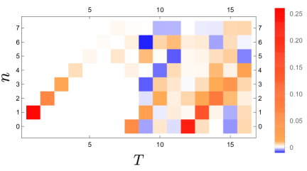
Figure 1: Non-zero non-local correlations on the self-dual line given by $C_{zy}^{zy}(n,T)=\operatorname{Tr}{U}^{T}\sigma_{1}^{z}\sigma_{0}^{y}{U}^{-T}\sigma_{n+1}^{z}\sigma_{n}^{y}$. Visible is the exponential decay along one side of the light-cone, exchanging $y\leftrightarrow z$ exchanges the direction. After $T\geq N-1$ additional correlations, and a revival, occur. The shown system features $N=8$ and $h=0.65362$.

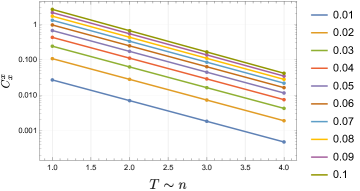
Figure 2: The behaviour of $C_{x}^{x}(n=T)=\operatorname{Tr}\big{(}U^{-T}\sigma_{T}^{x}{U}^{T}$ $\sigma_{1}^{x}\big{)}$ for $N=8$ spins with a generic value of $h=0.65362$. The system is near the self-dual line, i.e. $b=\pi/4$ and $J=\pi/4+\Delta J$. The figure shows the exponential decay with distance $n$, for various values of $\Delta J$, see legend. For $\Delta J\to 0$ the exponent is given by $\ln\cos{2h}\approx-1.35$, which holds in good approximation for all presented values of $\Delta J$.

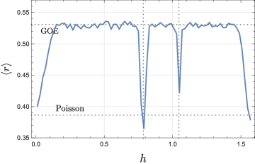
Figure 3: The figure shows the value of $r$ for the spectrum of the dual KIC at $N=15$ as a function of $h$ averaged over all values in the separate (translation) symmetry sectors of $k=1,\dots,7$. Note that the graph is symmetric under reflection $h\to\pi-h$. For most values of $h$ the data for $\langle r\rangle$ fit the GOE prediction. The four dips at $h=0,\pi/4,\pi/3,\pi$ correspond to spectral statistics characteristic of integrable systems.

VII Relation to dual-unitary circuit lattices

For the sake of comparison it is instructive to observe a connection between the dual quantum kicked chain and dual circuit lattices, studied in BeKoPr19-4 . Such a connection can be established when both the chain length $N$ and the propagation times $T$ are even. It is straightforward to see that the quantum evolution operator $U^{2T}$ for even times can be cast into the form

$$U^{2T}=U_{\scriptscriptstyle I}^{e}U_{\mathrm{circ}}^{T}(U_{\scriptscriptstyle I}^{e})^{\dagger}.$$ (34)

Here, the operator $U_{\scriptscriptstyle I}^{e}$ corresponds to the even half of the ”interaction”:

$$\langle\bm{s}|U_{\scriptscriptstyle I}^{e}[f_{1}]|\bm{s^{\prime}}\rangle=\delta(\bm{s},\bm{s^{\prime}})e^{i\sum_{n=1}^{N/2}f_{1}(s_{2n},s_{2n+1})},$$ (35)

and the evolution $U_{\mathrm{circ}}$ has the form

$$U_{\mathrm{circ}}=\mathbb{T}U_{\scriptscriptstyle I}^{e}U_{\scriptscriptstyle K}U_{\scriptscriptstyle I}^{e}\mathbb{T}^{\dagger}U_{\scriptscriptstyle I}^{e}U_{\scriptscriptstyle K}U_{\scriptscriptstyle I}^{e},$$ (36)

where $\mathbb{T}$ is the circular shift operator on a lattice of $N$ sites. Note that $U_{\mathrm{circ}}$ has a special structure, characteristic to circuit lattice evolution BeKoPr19-4 . The role of the unitary gate operator is fulfilled here by

$$U_{\mathrm{gate}}=u^{e}_{1}\,(u_{2}\otimes u_{2})\,u^{e}_{1},$$ (37)

where the diagonal matrix

$$\langle s_{1}s_{2}|u^{e}_{1}|s^{\prime}_{1}s^{\prime}_{2}\rangle=\delta(s_{1},{s^{\prime}}_{1})\delta(s_{2},{s^{\prime}}_{2})e^{if_{1}(s_{1},s_{2})}$$

is a restriction of $U_{\scriptscriptstyle I}^{e}$ to two adjacent lattice sites.

By eq. (36) we find for two-point correlator

$$\operatorname{Tr}\left(U^{T}Q_{1}U^{-T}Q_{2}\right)=\operatorname{Tr}\left(U_{\mathrm{circ}}^{T}\tilde{Q}_{1}U_{\mathrm{circ}}^{-T}\tilde{Q}_{1}\right),$$ (38)

where $\tilde{Q}_{i}=(U_{\scriptscriptstyle I}^{e})^{\dagger}Q_{i}U_{\scriptscriptstyle I}^{e}$. Since $U_{\scriptscriptstyle I}^{e}$ couples two neighbouring sites, any local operator in the kicked model corresponds to a two site operator of the respective circuit model and vice versa.

VIII Conclusions

We analyzed correlations between local operators in DuKC built upon a pair of $L\times L$ complex Hadamard matrices. The correlators of strictly local isolated traceless operators were shown to vanish identically for sufficiently long chains. On the other hand correlations between operators with a finite support were found to be, generically non-trivial along light-cone edges. Here an explicit formula, relating correlators to the expectation values of a transfer operator has been derived. For the subfamily of DFTC we go much further and obtain an explicit analytical expression for correlations between operators supported on pairs of adjacent sites. Furthermore, by using these results we were able to evaluate correlations between strictly local operators of KIC in the vicinity of the dual regime.

So far, we have discussed only homogeneous models. However, the results of the current paper can be straightforwardly extended to dual-unitary systems with spatial-temporal disorder. In such a case the transfer operator $\mathbf{T}^{n-2}$ is substituted with a product of local “gate” operators $\mathbf{T}_{1}\mathbf{T}_{2}\dots\mathbf{T}_{n-2}$, where each $\mathbf{T}_{i}$ depends on $f_{1},f_{2}$ at the relevant point of the spatial-temporal lattice. For DFTC all matrices $\mathbf{T}_{i}$ are diagonalized by one and the same unitary transformation. As a result, the decay exponents of the correlators (24) in the disordered case are just given by the averages of the local exponents. In particular, for the non-homogeneous KIC model one has $C(n,T)\sim\delta(n,T)\prod_{i=1}^{n-2}\cos 2h_{i}$, where the $h_{i}$’s are local magnetic fields at the corresponding points of the spatial-temporal lattice.

Several open questions deserve further studies. First, a possible extension of the above results to all DuKC models should be explored. Second, it would be of interest to investigate whether explicit results for correlations between operators with larger supports can be obtained for DFTC. Finally, the semiclassical limit $L\to\infty$ of DFTC deserves a separate study. The classical model emerging in this limit is nothing more than a (perturbed) coupled cat map lattice considered in GutOsi15 ; GHJSC16 . Depending on the functions $\lambda_{i}(s),\lambda^{\prime}_{i}(s)$ this model exhibits different dynamical behaviours in the classical limit, ranging from full chaos to full integrability. For a finite dimension $L$ of the local Hilbert space the two-point correlators of traceless operators decay exponentially provided the transfer operator contains no eigenvalues on the unite circle, except the trivial one (associated with the unit operator). Thus, independently of the underlying classical dynamics, for a fixed $L$ dual-unitary systems generically exhibit quantum chaos behavior in the thermodynamic limit $N\to\infty$, associated with the exponential decay of correlators. On the other hand, if the semiclassical limit $L\to\infty$ is taken first (or simultaneously with the thermodynamic limit) the gap in the transfer operator spectrum might close, such that no exponential decay is observed for any finite $N$. This shows that the emerging theory is very sensitive to the order of the thermodynamic and semiclassical limits.

p. 1

IX Supplementary material

IX.1 Dual representation of correlators

As the first step, we rewrite correlator (11) in the form of partition function for a classical statistical model. Specifically, we have

$$C_{1,2}=L^{-N}\operatorname{Tr}\left(U^{T}Q_{1}U^{-T}Q_{2}\right)=\frac{1}{L^{NT}}\sum_{\{s_{m,t}\in 1,\dots,L\}}e^{-i\mathcal{F}(\{s_{m,t}\})}\langle s_{n_{1},2T}|\mathbf{q}_{1}^{c}|s_{n_{1},1}\rangle\langle s_{n_{2},T}|\mathbf{q}_{2}|s_{n_{2},T+1}\rangle\\ \times\prod_{m\neq n_{1}}^{N-1}\delta(s_{m,2T},s_{m,1})\prod_{m\neq n_{2}}^{N-1}\delta(s_{m,T},s_{m,T+1}),$$

where

$$\mathcal{F}=\sum_{t=1}^{T}\sum_{m=0}^{N-1}f_{1}(s_{m,t},s_{m+1,t})-f_{1}(s_{m,t+T},s_{m+1,t+T})+f_{2}(s_{m+1,t},s_{m,t})-f_{2}(s_{m,t+T},s_{m+1,t+T}).$$ (39)

The last expression can be rewritten through the transfer operators in the spatial direction as

$$C_{1,2}=\operatorname{Tr}\big{(}W^{N+n_{1}-n_{2}-1}\overline{W}_{{\mathbf{q}}_{1}}W^{n_{2}-n_{1}-1}W_{\mathbf{q}_{2}}\big{)}.$$

if $n_{1}\neq n_{2}$ and

$$C_{1,2}=\operatorname{Tr}\big{(}W^{N-1}W_{\mathbf{q}_{1}\mathbf{q}_{2}}\big{)}$$ (40)

if $n_{1}=n_{2}$.

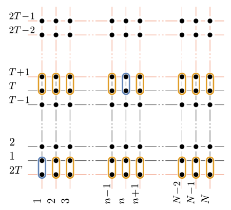
Figure 4: The figure illustrates eq. (11). The first and the n-th vertical line corresponds to the operators $\overline{W}_{\bar{\mathbf{q}}_{1}}$ and $W_{\mathbf{q}_{2}}$, respectively. The intermediate lines correspond to the operator $W$.

The dual representation has a natural extension to $l$-point correlator (48). Assuming that all points are ordered, $t_{l}>t_{l-1}>\dots>t_{1}$, $n_{l}>n_{l-1}>\dots>n_{1}$ we have

$$C_{1,\dots,l}=\operatorname{Tr}\big{(}W^{N+n_{1}-n_{l}-1}W_{1}W^{\Delta n_{1}}W_{2}W^{\Delta n_{2}}\dots W_{l}\big{)},$$ (41)

where $\Delta n_{i}=n_{i+1}-n_{i}-1$. Here $W_{1}=\overline{W}_{{\mathbf{q}}_{1}},W_{l}=W_{{\mathbf{q}}_{l}}$, and $W_{k}=W_{\scriptscriptstyle I}^{(k)}[\mathbf{q}_{k}]W_{\scriptscriptstyle K}$, for $1<k<l$ with

$$\langle\bm{s}|W_{\scriptscriptstyle I}^{k}[\mathbf{a}]|{\bm{s}^{\prime}}\rangle=\langle s_{k}|\mathbf{a}|s_{k+1}\rangle\delta(s_{1},s_{2T})\delta(s_{T},s_{T+1})\delta(\bm{s},{\bm{s}^{\prime}})e^{{\left(-i\sum_{t=1}^{T-1}f_{2}(s_{t+1},s_{t})+i\sum_{t=T+1}^{2T-1}f_{2}(s_{t},s_{t+1})\right)}}.$$ (42)

IX.2 Proof of Proposition 1

In this section we are going to prove eq. 18. which in the matrix form can be written as

$$\langle\bm{\eta}|W^{T}|\bm{\eta}^{\prime}\rangle\sim\prod_{t=1}^{T}\delta(\eta_{t}-\eta_{T-t+1})\delta(\eta^{\prime}_{t}-\eta^{\prime}_{T-t+1}).$$ (43)

In order to prove this relation it is instructive to write down the left hand side of (43) in the form of partition function

$$\langle\bm{\eta}|W^{T}|\bm{\eta}^{\prime}\rangle=\frac{1}{L^{NT}}\sum_{\{s_{n,t}\}}e^{i\left(\mathcal{F}_{1}(\{s_{n,t}\})+\mathcal{F}_{2}(\bm{\eta},\bm{\eta}^{\prime})\right)}\prod_{n=1}^{N}\delta(s_{n,T}-s_{n,T+1})\delta(s_{n,2T}-s_{n,1}),$$ (44)

where the sum is over $NT$ variables $s_{n,t}$ with

$$\mathcal{F}_{1}=\sum_{t=1}^{T}\sum_{n=1}^{N-1}f_{1}(s_{n,t},s_{n+1,t})-f_{1}(s_{n,t+T},s_{n+1,t+T})+f_{2}(s_{n,t},s_{n+1,t})-f_{2}(s_{n,t+T},s_{n+1,t+T}),$$ (45)

$$\mathcal{F}_{2}=\sum_{t=1}^{T}f_{1}(\eta_{t},s_{1,t})-f_{1}(\eta_{t+T},s_{1,t+T})+f_{1}(\eta^{\prime}_{t},s_{N,t})-f_{1}(\eta^{\prime}_{t+T},s_{N,t+T}).$$ (46)

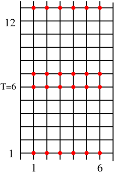
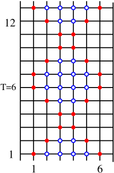
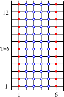
Figure 5: Two step elimination process of the summation variables in the partition function. At the left picture is illustrated the initial expression, where summation is ran over $N\cdot 2T$ variables $s_{n,t}$. Dots in red show the spins which are paired by the condition $s_{n,t}=s_{n,2T-t+1}$. At the first step all the variables $s_{n,t}$ within the light cone are summed up (eliminated). They are shown by the blue (empty) circles in the middle figure. At the second step the variables $s_{n,t}$ outside of the light cone are eliminated, as illustrated at the right figure.

The summation over the set of integers $s_{n,t}$ is performed then in two steps. At first all the variables within light cone are eliminated one by one as shown in fig. 5. Then at the second step the summation variables $s_{n,t}$ outside of the light cone are eliminated except the first and the last raw. This yields

$$\langle\bm{\eta}|W^{T}|\bm{\eta}^{\prime}\rangle\sim\frac{1}{L^{NT}}\sum_{\{s_{1,t},s_{N,t}\}}e^{i\mathcal{F}_{2}(\{s_{1,t},s_{N,t},\eta_{t},\eta_{t}^{\prime}\})}\prod_{t=1}^{N}\delta(s_{1,t}-s_{1,2T-t+1})\delta(s_{N,t}-s_{N,2T-t+1}),$$ (47)

which after taking the sum gives (43).

IX.3 $l$-point correlations between strictly local operators.

Let $Q(z_{i})=U_{\scriptscriptstyle N}^{-t_{i}}Q_{i}U_{\scriptscriptstyle N}^{t_{i}}$, $z_{i}=(n_{i},t_{i})$ be a set of local traceless operators supported at the ordered sites $z_{1},\dots,z_{l}$ of the spacial-temporal lattice i.e., $t_{l}>t_{l-1}>\dots>t_{1}$, $n_{l}>n_{l-1}>\dots>n_{1}$. We are going to show that their correlations,

$$C_{1,\dots,l}=L^{-N}\operatorname{Tr}\big{(}Q_{1}(z_{1})Q_{2}(z_{2})\dots Q_{l}(z_{l})\big{)},$$ (48)

vanish identically for $N>|t_{l}-t_{1}|+|n_{l}-n_{1}|$, under the condition that all operators $Q_{i}$ are isolated from each other, i.e. $|n_{i}-n_{i+1}|>1$ for all $i=1,\dots,l$. In the dual representation

$$C_{1,\dots,l}=\operatorname{Tr}\big{(}W^{N-n_{l}+n_{1}-1}W_{1}W^{\Delta n_{1}}W_{2}W^{\Delta n_{2}}\dots W_{l}\big{)},$$ (49)

where $\Delta n_{i}=n_{i+1}-n_{i}-1$. Here $W_{1}=\overline{W}_{{\mathbf{q}}_{1}},W_{l}=W_{{\mathbf{q}}_{l}}$, and $W_{k}$, $1<k<l$, defined by eq. (42), have dimensions $L^{2T}$, $T=t_{l}-t_{1}$. By applying Propositions 1, 2 we get $C_{1,\dots,l}=0$ for traceless operators.

For general operators $Q_{i}$ we can again use the decomposition (22). Under the condition that all operators are isolated and spatial temporal ordered, one has

$$\langle\prod_{i=1}^{l}Q_{i}(z_{i})\rangle=\prod_{i=1}^{l}\langle Q_{i}\rangle.$$ (50)

IX.4 Correlations between operators with two-point support

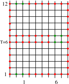
Figure 6: Elimination of the summation variables in the partition function representing 4-point correlator for $T=6$. At the left picture is illustrated the initial expression, where the sum runs over $(N+2)\cdot 2T$ variables $s_{n,t}$. Dots in red show the variables which are paired by the condition $s_{n,t}=s_{n,2T-t+1}$. At the right picture is shown partition function after elimination of $s_{n,t}$, shown by blue circles. The remaining sum along the light-cone edge can be represented in the form of the expectation value (52) of the $L^{2}\times L^{2}$ transfer operator $\mathbf{T}$.

Here we consider the two point correlator of pairs of operators:

$$C(n,T)=L^{-N}\operatorname{Tr}U^{T}\Sigma_{0}U^{-T}\Sigma_{n}$$ (51)

$$\Sigma_{0}=Q_{1}(0)Q_{2}(1),\qquad\Sigma_{n}=Q_{3}(n)Q_{4}(n+1)$$

at the cone light border $n=T$. It is instructive to represent $C_{T}=C(n=T,T)$ in the form of partition function. The initial expression is shown in a graphic form on the left hand side of fig.  6. The summation variables $s_{n,t}$ are excluded one by one up to reaching the stage illustrated by the right hand figure. Here the summation variables (shown in red and black) are located along one dimensional strip only, which reduces the whole problem to calculation of quasi-one dimensional partition function. Explicitly it can be cast into the form:

$$C_{T}=\langle\bar{\Phi}_{\mathbf{q}_{1}\mathbf{q}_{2}}|\mathbf{T}^{T-2}|\Phi_{\mathbf{q}_{3}\mathbf{q}_{4}}\rangle,$$ (52)

where the left $\bar{\Phi}_{\mathbf{q}_{1}\mathbf{q}_{2}}$ and the right $\Phi_{\mathbf{q}_{3}\mathbf{q}_{4}}$ vectors are defined as

$$\langle\nu\eta|\Phi_{\mathbf{q}_{3}\mathbf{q}_{4}}\rangle = \frac{1}{L^{3}}\sum_{a,\bar{a},b=1}^{L}e^{i(f_{1}(\eta,\bar{a})-f_{1}(\eta,a)+f_{2}(\bar{a},\nu)-f_{2}(a,\nu)-f_{1}(a,b)+f_{1}(\bar{a},b))}\langle a|\mathbf{q}_{3}|\bar{a}\rangle\langle b|\mathbf{q}_{4}|b\rangle,$$ (53)

$$\langle\bar{\Phi}_{{\mathbf{q}}_{1}{\mathbf{q}}_{2}}|\eta\nu\rangle = \frac{1}{L^{3}}\sum_{a,\bar{a},b=1}^{L}e^{i(f_{1}(a,\nu)-f_{1}(\bar{a},\nu)+f_{2}(\eta,a)-f_{2}(\eta,\bar{a})+f_{1}(b,a)-f_{1}(b,\bar{a}))}\langle a|u_{2}{\mathbf{q}}_{2}u^{\dagger}_{2}|\bar{a}\rangle\langle b|u_{2}{\mathbf{q}}_{1}u^{\dagger}_{2}|b\rangle,$$ (54)

and the transfer operator $\mathbf{T}$,

$$\langle\nu\eta|\mathbf{T}|\eta^{\prime}\nu^{\prime}\rangle=\frac{1}{L^{3}}\left|\sum_{s=1}^{L}e^{i(f_{1}(\eta,s)+f_{1}(s,\nu^{\prime})+f_{2}(\nu,s)+f_{2}(s,\eta^{\prime}))}\right|^{2},$$ (55)

acting on the small space $\mathcal{H}\otimes\mathcal{H}$.

It is easy to check that $\mathbf{T}$ is doubly stochastic operator i.e, satisfies

$$\sum_{\nu=1}^{L}\sum_{\eta=1}^{L}\langle\nu\eta|\mathbf{T}|\eta^{\prime}\nu^{\prime}\rangle=1.$$ (56)

This implies that the spectrum of $\mathbf{T}$ is contained within the unit disc with at least one eigenvalue equal to $1$ corresponding to uniform eigenvector.

IX.5 Application to DFTC model

By eq. (52) we have

$$C_{T}=\sum_{m=0}^{\lfloor L/2\rfloor}(\mathbf{t}_{m})^{T-2}\left(2-\delta_{m,0}-\delta_{m,\frac{L}{2}}\right)\mathrm{Re}[A_{m}(\mathbf{q}_{4})\langle\bar{\Phi}_{\mathbf{q}_{1}\mathbf{q}_{2}}|\Phi_{\mathbf{q}_{3}\mathbf{e}_{m}}\rangle],$$ (57)

for even $T$ and

$$C_{T}=\sum_{m=0}^{\lfloor L/2\rfloor}(\mathbf{t}_{m})^{T-2}\left(2-\delta_{m,0}-\delta_{m,\frac{L}{2}}\right)\mathrm{Re}[e^{-i\phi}A^{*}_{m}(\mathbf{q}_{4})\langle\bar{\Phi}_{\mathbf{q}_{1}\mathbf{q}_{2}}|\Phi_{\mathbf{q}_{3}\mathbf{e}_{m}}\rangle],$$ (58)

for odd $T$, where

$$A_{m}(\mathbf{q})=\frac{1}{L}\sum_{s=1}^{L}e^{i2\pi sm/L}\langle s|\mathbf{q}|s\rangle.$$

The scalar products $\langle\bar{\Phi}_{\mathbf{q}_{1}\mathbf{q}_{2}}|\Phi_{\mathbf{q}_{3}\mathbf{e}_{m}}\rangle$ can be easily evaluated by using eqs. (53, 54)

$$\langle\bar{\Phi}_{\mathbf{q}_{1}\mathbf{q}_{2}}|\Phi_{\mathbf{q}_{3}\mathbf{e}_{m}}\rangle=A_{m}(\mathbf{q}^{c}_{1})B^{(1)}_{m}(\mathbf{q}_{3})B^{(2)}_{m}(\mathbf{q}^{c}_{2}),\quad B^{(j)}_{m}(\mathbf{q})=\frac{1}{L}\sum_{s=1}^{L}e^{i(\mu_{j}(s)-\mu_{j}(s^{(m)}))}\langle s|\mathbf{q}|s^{(m)}\rangle,\quad j=1,2$$ (59)

with $s^{(m)}=1+(s+m-1)\!\!\mod L$, and $\mu_{1}(s)=-\lambda_{1}(s)-\lambda^{\prime}_{1}(s)-\lambda_{2}(s)$ and $\mu_{2}(s)=\lambda_{1}(s)+\lambda^{\prime}_{1}(s)+\lambda^{\prime}_{2}(s)$, respectively. Note that the constants $A_{m}(\mathbf{q}),B^{(j)}_{m}(\mathbf{q})$ can be also written in a more compact form as

$$A_{m}(\mathbf{q})=\frac{1}{L}\operatorname{Tr}\left(\Gamma^{m}_{0}\mathbf{q}\right),\qquad B^{(j)}_{m}(\mathbf{q})=\frac{1}{L}\operatorname{Tr}\left(\Gamma_{j}\mathbf{q}\Gamma_{j}^{\dagger}\,\mathbb{T}^{m}\right),$$ (60)

where $\mathbb{T}$ is the circular shift operator, $\mathbb{T}|s\rangle=|s^{(m)}\rangle$, and $\Gamma_{j},j=1,2,3$ are the diagonal matrices:

$$\Gamma_{0}=\mbox{diag}\{e^{i2\pi s/L}\}_{s=1}^{L},\qquad\Gamma_{j}=\mbox{diag}\{e^{i\mu_{j}(s)}\}_{s=1}^{L},\qquad j=1,2.$$ (61)

IX.6 Application to KIC model

The KIC model provides a minimal realisation of self-dual models with $L=2$. The KIC evolution is governed by the Hamiltonians:

$$H_{\scriptscriptstyle I}=\sum_{n=1}^{N}J\sigma_{n}^{z}\sigma_{n+1}^{z}+h\sigma_{n}^{z},\qquad H_{\scriptscriptstyle K}=b\sum_{n=1}^{N}\sigma_{n}^{x},$$ (62)

where $\sigma_{n}^{\alpha},\alpha=x,y,z$ are Pauli matrices. The dual case corresponds to $J=b=\pi/4$ with $h$ being arbitrary. The resulting evolutions $U_{\scriptscriptstyle K}$, $U_{\scriptscriptstyle I}$ take the form (5) with the functions

$$f_{1}=-\frac{\pi}{4}mn-\frac{h}{2}(m+n),\qquad f_{2}=\frac{\pi}{4}(mn-1),$$

$m,n=\pm 1$, defining the two unitary matrices $u_{1},u_{2}$:

$$u_{1}=\frac{1}{\sqrt{2}}\begin{pmatrix}e^{-i(\frac{\pi}{4}+h)}&e^{i\frac{\pi}{4}}\\ e^{i\frac{\pi}{4}}&e^{-i(\frac{\pi}{4}-h)}\end{pmatrix},\qquad u_{2}=\frac{1}{\sqrt{2}}\begin{pmatrix}1&-i\\ -i&1\end{pmatrix}.$$ (63)

Note that $u_{1},u_{2}$ can be expressed through the DFT matrix $F$ as:

$$u_{1}=\begin{pmatrix}e^{-\frac{ih}{2}}&0\\ 0&e^{\frac{i(\pi+h)}{2}}\end{pmatrix}F\begin{pmatrix}e^{-\frac{i(\pi+2h)}{4}}&0\\ 0&e^{\frac{i(\pi+2h)}{4}}\end{pmatrix},\quad u_{2}=\begin{pmatrix}1&0\\ 0&e^{-\frac{i\pi}{2}}\end{pmatrix}F\begin{pmatrix}1&0\\ 0&e^{-\frac{i\pi}{2}}\end{pmatrix},\quad F=\frac{1}{\sqrt{2}}\begin{pmatrix}1&1\\ 1&-1\end{pmatrix}.$$

This implies that KIC is just a particular case of the DFTC model for $L=2$ with the parameters

$$\Lambda_{1}=\mbox{diag}\{e^{-i{h}/{2}},e^{i(\pi+h)/2}\},\quad\Lambda^{\prime}_{1}=\mbox{diag}\{e^{-i(\pi+2h)/{4}},e^{i(\pi+2h)/4}\},\quad\Lambda_{2}=\Lambda^{\prime}_{2}=\mbox{diag}\{1,e^{-i\pi/2}\}.$$ (64)

For the KIC model both the transfer operator (55) and the vectors (53, 54) can be calculated explicitly. Inserting into eq. (55) the corresponding functions $f_{1},f_{2}$ yields:

$$\mathbf{T}=\frac{1}{2}\begin{pmatrix}a&b&b&a\\ b&a&a&b\\ b&a&a&b\\ a&b&b&a\end{pmatrix},$$ (65)

where $a=\cos^{2}h$, $b=\sin^{2}h$. The four eigenvalues of this matrix are $\{1,\cos 2h,0,0\}$ in agreement with the results of BeKoPr19-4 .

To evaluate correlators note that the operators $u_{2}{\mathbf{q}}_{1}u^{\dagger}_{2},\mathbf{q}_{4}$ contribute only diagonal elements into (53,54). In the case of KIC model this means that only the spin combinations, $\Sigma_{0}=\sigma^{y}_{0}\sigma^{j}_{1}$, $\Sigma_{n}=\sigma^{i}_{n}\sigma^{z}_{n+1}$ might have non-trivial correlations. The corresponding vectors are given by:

$$\Phi_{\sigma_{y},\sigma_{z}}=\bar{\Phi}_{\sigma_{y},\sigma_{z}}=\Phi_{0}\cos 2h,$$ (66)

$$\Phi_{\sigma_{x},\sigma_{z}}=\bar{\Phi}_{\sigma_{y},\sigma_{x}}=-\Phi_{0}\sin 2h,$$ (67)

with $\Phi_{0}=\frac{1}{2}(1,-1,-1,1)^{T}$ being the eigenvector of ${\mathbf{T}}$ for the eigenvalue $\cos 2h$. All other combinations of $x,y,z$ give rise to zero vectors. After inserting (65,66,67) into (52) we obtain

$$C_{T}=\mathcal{C}\cos^{T}2h,$$ (68)

where prefactors $\mathcal{C}=\mathcal{C}(\sigma_{0}^{i}\sigma_{1}^{j},\sigma_{n}^{k}\sigma_{n+1}^{m})$ are given by

$$\mathcal{C}(\sigma_{0}^{y}\sigma_{1}^{z},\sigma_{n}^{y}\sigma_{n+1}^{z})=1,\qquad\mathcal{C}(\sigma_{0}^{y}\sigma_{1}^{x},\sigma_{n}^{x}\sigma_{n+1}^{z})=\tan^{2}2h$$ (69)

$$\mathcal{C}(\sigma_{0}^{y}\sigma_{1}^{x},\sigma_{n}^{y}\sigma_{n+1}^{z})=\mathcal{C}(\sigma_{0}^{y}\sigma_{1}^{z},\sigma_{n}^{x}\sigma_{n+1}^{z})=-\tan 2h$$ (70)

while zeroes for all other spin combinations. The same result can be also obtained straightforwardly from the general result (57,57) on the DFTC model.

The correlator (68) decays exponentially for any value of $h$ except for the set of integrable points $h=\frac{1}{4}\pi k,k\in\mathbb{Z}$, where the subleading eigenvalue of $\mathbf{T}$ has absolute value one. In particular, for $h=0$ the correlator (31) vanishes everywhere except for the cone border, where it remains constant and does not decay (also for $N<T$). For $h=\pi/4$ the correlator vanishes everywhere except for revivals at $N=T$.

IX.7 Two-point correlator in non-dual KIC model

While the two point correlator of strictly local operators vanishes everywhere in the dual regime it stays finite as soon as $J-\pi/4=\Delta J\neq 0$. Below we evaluate

$$C_{x}^{x}(n=T,J)=\operatorname{Tr}\left(U_{J}^{-T}\sigma_{n}^{x}{U}_{J}^{T}\sigma_{1}^{x}\right),$$ (71)

to the leading order of $\Delta J$:

$$C_{x}^{x}(n=T,J)=C_{1}\Delta J+(C_{2}/2)(\Delta J)^{2}+O\left((\Delta J)^{4}\right).$$ (72)

As $C_{1}=0$, we need to evaluate

$$C_{2}=\frac{d^{2}}{dJ^{2}}\operatorname{Tr}\left(U_{J}^{-T}\sigma_{n}^{x}{U}_{J}^{T}\sigma_{1}^{x}\right)\Big{|}_{J=\pi/4}.$$ (73)

A straightforward calculation gives

$$C_{2}=2\sum_{k=0}^{m-1}\sum_{m=1}^{T-1}\operatorname{Tr}\left([H_{\scriptscriptstyle I}^{0}(k),\sigma_{1}^{x}][H_{\scriptscriptstyle I}^{0}(m)\sigma_{n}^{x}(T)]\right)+\sum_{m=1}^{T}\operatorname{Tr}\left([H_{\scriptscriptstyle I}^{0}(m),\sigma_{1}^{x}][H_{\scriptscriptstyle I}^{0}(m)\sigma_{n}^{x}(T)]\right),$$ (74)

where

$$\sigma_{n}^{x}(T)=U^{-T}\sigma_{n}^{x}U^{T},\qquad H_{\scriptscriptstyle I}^{0}(m)=U^{-m}\left(\sum_{n=1}^{N}\sigma_{n}^{z}\sigma_{n+1}^{z}\right)U^{m}.$$

For $n=T$ only the first term in the above sum provides the non-trivial contribution:

$$C_{2}=2\operatorname{Tr}\left([H_{\scriptscriptstyle I}^{0},\sigma_{1}^{x}][H_{\scriptscriptstyle I}^{0}(n-1),\sigma_{n}^{x}(n)]\right)=8\operatorname{Tr}\left(U^{-n}\sigma_{n}^{y}\sigma_{n+1}^{z}{U}^{n}\sigma_{0}^{y}\sigma_{1}^{z}\right)=8\cos^{n}2h.$$ (75)

References

- (1) T. Engl, J. Dujardin, A. Argüelles, P. Schlagheck, K. Richter, and J. D. Urbina, “Coherent backscattering in fock space: A signature of quantum many-body interference in interacting bosonic systems,” Phys. Rev. Lett., vol. 112, p. 140403, Apr 2014.
- (2) R. Dubertrand and S. Müller, “Spectral statistics of chaotic many-body systems,” New Journal of Physics, vol. 18, p. 033009, mar 2016.
- (3) P. Ponte, Z. Papić, F. Huveneers, and D. A. Abanin, “Many-body localization in periodically driven systems,” Phys. Rev. Lett., vol. 114, p. 140401, Apr 2015.
- (4) Y. Y. Atas and E. Bogomolny, “Spectral density of a one-dimensional quantum Ising model: Gaussian and multi-Gaussian approximations,” Journal of Physics A: Mathematical and Theoretical, vol. 47, p. 335201, aug 2014.
- (5) J. P. Keating, N. Linden, and H. J. Wells, “Spectra and Eigenstates of Spin Chain Hamiltonians,” Communications in Mathematical Physics, vol. 338, p. 81–102, Aug 2015.
- (6) S. Czischek, M. Gärttner, M. Oberthaler, M. Kastner, and T. Gasenzer, “Quenches near criticality of the quantum Ising chain—power and limitations of the discrete truncated Wigner approximation,” Quantum Science and Technology, vol. 4, p. 014006, oct 2018.
- (7) M. Schreiber, S. S. Hodgman, P. Bordia, H. P. Lüschen, M. H. Fischer, R. Vosk, E. Altman, U. Schneider, and I. Bloch, “Observation of many-body localization of interacting fermions in a quasirandom optical lattice,” Science, vol. 349, no. 6250, p. 842–845, 2015.
- (8) J. Simon, W. S. Bakr, R. Ma, M. E. Tai, P. M. Preiss, and M. Greiner, “Quantum simulation of antiferromagnetic spin chains in an optical lattice,” Nature, vol. 472, no. 7343, p. 307–312, 2011.
- (9) M. Akila, D. Waltner, B. Gutkin, and T. Guhr, “Particle-time duality in the kicked Ising spin chain,” J. Phys. A, vol. 49, p. 375101, 2016.
- (10) M. Akila, D. Waltner, B. Gutkin, P. Braun, and T. Guhr, “Semiclassical identification of periodic orbits in a quantum many-body system,” Phys. Rev. Lett., vol. 118, p. 164101, 2017.
- (11) M. Akila, B. Gutkin, P. Braun, D. Waltner, and T. Guhr, “Semiclassical prediction of large spectral fluctuations in interacting kicked spin chains,” Ann. Phys., vol. 389, pp. 250–282, 2018.
- (12) B. Gutkin and V. Osipov, “Classical foundations of many-particle quantum chaos,” Nonlinearity, vol. 29, pp. 325–356, 2016.
- (13) B. Gutkin, L. Han, R. Jafari, A. K. Saremi, and P. Cvitanović, “Linear encoding of the spatiotemporal cat map,” 2019. arXiv:1912.02940.
- (14) B. Bertini, P. Kos, and T. Prosen, “Exact spectral form factor in a minimal model of many-body quantum chaos,” Phys. Rev. Lett., vol. 121, p. 264101, 2018.
- (15) B. Bertini, P. Kos, and T. Prosen, “Entanglement spreading in a minimal model of maximal many-body quantum chaos,” Phys. Rev. X, vol. 9, p. 021033, 2019.
- (16) P. Braun, D. Waltner, M. Akila, B. Gutkin, and T. Guhr, “Transition from quantum chaos to localization in spin chains,” 2019. arXiv:1902.06265.
- (17) R. Pal and A. Lakshminarayan, “Entangling power of time-evolution operators in integrable and nonintegrable many-body systems,” Phys. Rev. B, vol. 98, p. 174304, Nov 2018.
- (18) B. Bertini, P. Kos, and T. Prosen, “Exact correlation functions for dual-unitary lattice models in dimensions,” Phys. Rev. Lett., vol. 123, p. 210601, Nov 2019.
- (19) S. Gopalakrishnan and A. Lamacraft, “Unitary circuits of finite depth and infinite width from quantum channels,” Phys. Rev. B, vol. 100, p. 064309, 2019.
- (20) B. Bertini, P. Kos, and T. Prosen, “Operator entanglement in local quantum circuits I: Maximally chaotic dual-unitary circuits,” 2019. arXiv:1909.07407.
- (21) J. Avan, V. Caudrelier, A. Doikou, and A. Kundu, “Lagrangian and hamiltonian structures in an integrable hierarchy and space-time duality,” Nuclear Physics B, vol. 902, pp. 415 – 439, 2016.
- (22) L. Piroli, B. Bertini, J. I. Cirac, and T. Prosen, “Exact dynamics in dual-unitary quantum circuits,” 2019. arXiv:1911.11175.
- (23) Z. Krajnik and T. Prosen, “Kardar-Parisi-Zhang physics in integrable rotationally symmetric dynamics on discrete space-time lattice,” 2019. arXiv:1909.03799.
- (24) T. Zhou and A. Nahum, “The entanglement membrane in chaotic many-body systems,” 2019. arXiv:1912.12311.
- (25) W. Tadej and K. Życzkowski, “A concise guide to complex hadamard matrices,” Open Systems & Information Dynamics, vol. 13, pp. 133–177, Jun 2006.
- (26) V. Oganesyan and D. A. Huse, “Localization of interacting fermions at high temperature,” Phys. Rev. B, vol. 75, p. 155111, Apr 2007.
- (27) Y. Y. Atas, E. Bogomolny, O. Giraud, and G. Roux, “Distribution of the ratio of consecutive level spacings in random matrix ensembles,” Phys. Rev. Lett., vol. 110, p. 084101, Feb 2013.
- (28) C. N. Yang and T. D. Lee, “Statistical theory of equations of state and phase transitions. i. theory of condensation,” Phys. Rev., vol. 87, pp. 404–409, Aug 1952.
- (29) T. D. Lee and C. N. Yang, “Statistical theory of equations of state and phase transitions. ii. lattice gas and ising model,” Phys. Rev., vol. 87, pp. 410–419, Aug 1952.
- (30) V. Matveev and R. Shrock, “On properties of the ising model for complex energy/temperature and magnetic field,” Journal of Physics A: Mathematical and Theoretical, vol. 41, p. 135002, mar 2008.
- (31) E. B. Bogomolny, B. Georgeot, M.-J. Giannoni, and C. Schmit, “Chaotic billiards generated by arithmetic groups,” Phys. Rev. Lett., vol. 69, pp. 1477–1480, Sep 1992.