General Partial Label Learning via Dual Bipartite Graph Autoencoder

Abstract

We formulate a practical yet challenging problem: General Partial Label Learning (GPLL). Compared to the traditional Partial Label Learning (PLL) problem, GPLL relaxes the supervision assumption from instance-level — a label set partially labels an instance — to group-level: 1) a label set partially labels a group of instances, where the within-group instance-label link annotations are missing, and 2) cross-group links are allowed — instances in a group may be partially linked to the label set from another group. Such ambiguous group-level supervision is more practical in real-world scenarios as additional annotation on the instance-level is no longer required, e.g., face-naming in videos where the group consists of faces in a frame, labeled by a name set in the corresponding caption. In this paper, we propose a novel graph convolutional network (GCN) called Dual Bipartite Graph Autoencoder (DB-GAE) to tackle the label ambiguity challenge of GPLL. First, we exploit the cross-group correlations to represent the instance groups as dual bipartite graphs: within-group and cross-group, which reciprocally complements each other to resolve the linking ambiguities. Second, we design a GCN autoencoder to encode and decode them, where the decodings are considered as the refined results. It is worth noting that DB-GAE is self-supervised and transductive, as it only uses the group-level supervision without a separate offline training stage. Extensive experiments on two real-world datasets demonstrate that DB-GAE significantly outperforms the best baseline over absolute 0.159 F1-score and 24.8% accuracy. We further offer analysis on various levels of label ambiguities.

Introduction

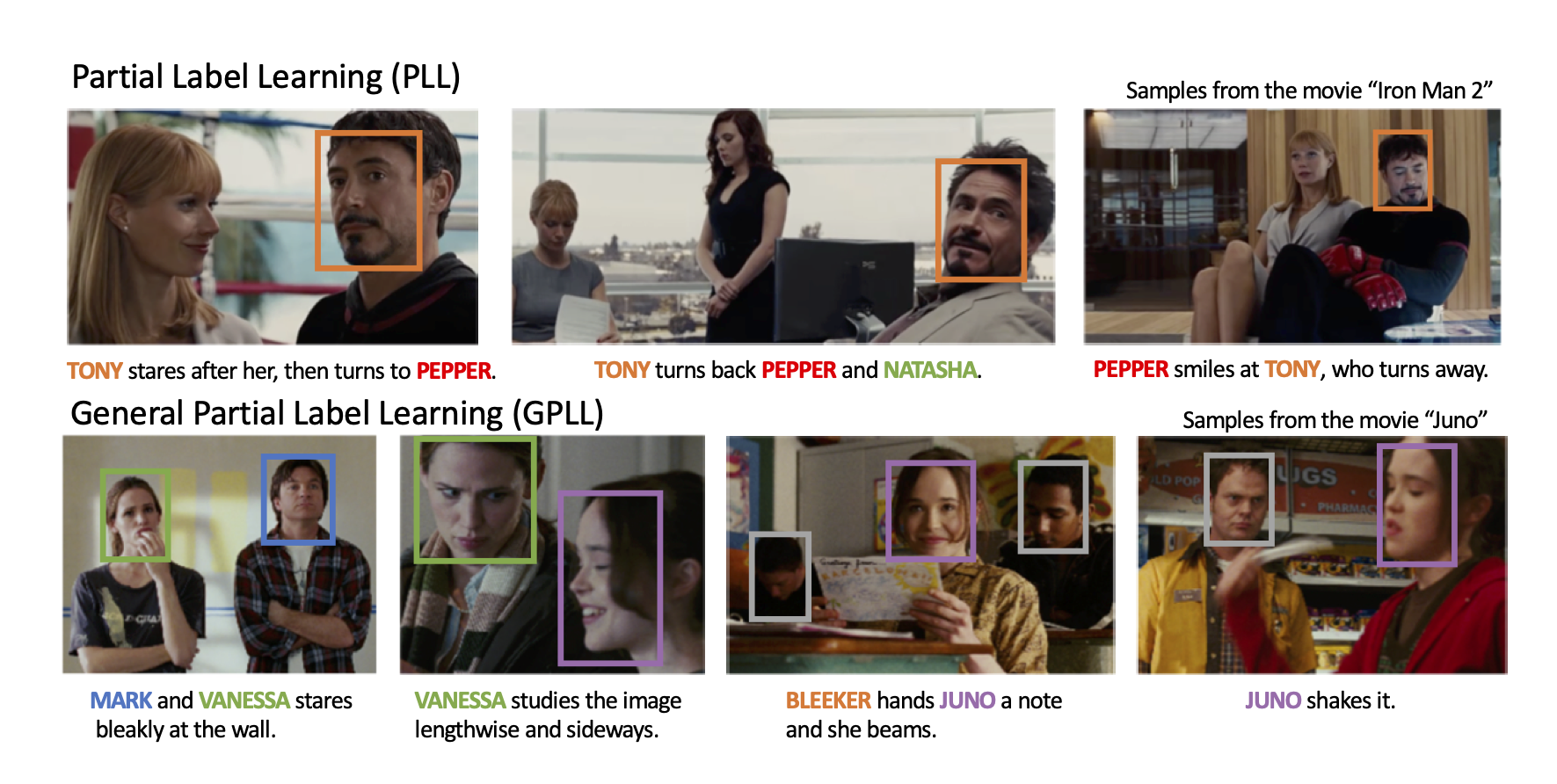
Figure 1: Top: Traditional PLL problem — each face is associated with one of the names in the caption. Bottom: The proposed GPLL problem addressed in this paper — there are general cases of faces without names or names without faces. See Figure 2 for illustrative formulation differences. Images are from MPII-MD  (?) and M-VAD  (?)

Labels are not always clean, complete, and unequivocal. As illustrated in Figure 1 (top), given a training instance , it corresponds to a candidate label set [,] where only one of them is correct. Learning from such ambiguous labels is known as Partial Label Learning (PLL) (?), which is a practical problem since it significantly reduces the human label effort compared to other one-to-one supervisions.

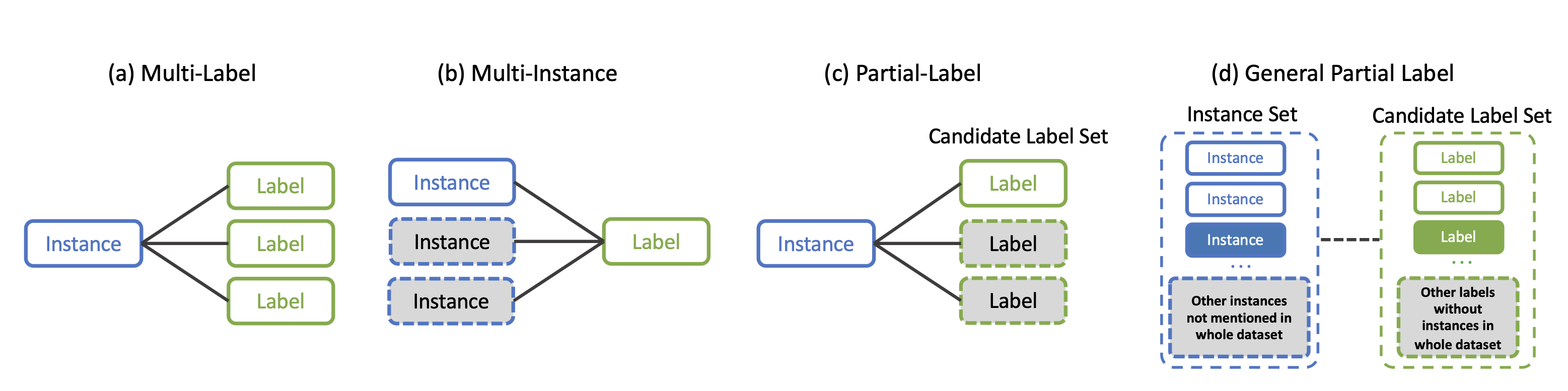
Figure 2: From (a) to (d), on the evolution of relaxing the supervision but bringing in more label ambiguity challenges. (a) Multi-Label (?): each instance is labeled with more than one labels. (b) Multi-Instance (?): at least one instance in a group belongs to the label. (c) Partial-Label (?): a candidate label set partially labels an instance, only one of them is correct. Note that the label set may vary from instance to instance. So far, the supervision is on instance-level. (d) General Partial Label Learning (our focus): group-level supervision. Instances or labels (blue or green shaded) may link to another group; there are also null instances and labels (grey shaded) with no links at all.

However, the assumption of PLL is still hardly feasible in large-scale scenarios: if we have millions of frames in videos or Web images, the instance-level label annotation of PLL will be prohibitively expensive. Figure 1 (bottom) shows several examples of the relaxation from instance-level to group-level: a group of instances and the candidate label set [,]. Compared to the tradition PLL, this is more complex and ambiguous: 1) within-group annotations are dropped, 2) cross-group links are allowed — appears in the candidate label set of another group [], and 3) there are some instances with $null$ label that is not in any label set. Such relaxed supervision is more appealing since it requires NO extra annotation on the instance-level. To this end, we propose a novel problem: General Partial Label Learning (GPLL), whose training annotation only comes from the inherent data pair (Figure 1 bottom), and thus is very challenging. Figure 2 illustrates some related problems with progressively relaxed supervisions.

A straightforward approach to GPLL is to consider some within-/cross-group heuristics such as : 1) Instances with similar features across groups likely belong to the same label. 2) Similar instances co-occur with the same label across groups implies that the label is likely assigned to those instances. 3) An instance cannot belong to multi-labels $\rightarrow$ , $\rightarrow$ , and distinct instances cannot be the same label within a group. However, these heuristics are too weak to address the extreme ambiguity. In fact, as we will show in Ablation Study, modeling such heuristics to construct the initial links only achieves 62.9% accuracy.

We believe that the key to solve GPLL is how to exploit the aforementioned cross-group correlations unsupervisedly to construct initial links and then refine them with stronger group contextual representations. To this end, we propose a novel graph convolutional network, called Dual Bipartite Graph Autoencoder (DB-GAE). As its name implies, DB-GAE explicitly learns richer within-group and cross-group representations which serve as a reciprocal complement to each other. The within-group representation resolves the ambiguity in a group, and the cross-group one renders additional global group context for further disambiguation. In particular, we first represent the initial links as the proposed within-group and cross-group bipartite graphs, and then use GCN (?) to encode and decode them to refine the dual links to obtain the results, where the reconstruction loss is only referenced to the within-group graph input as this is the only supervision we have in GPLL. Therefore, it is worth noting that DB-GAE is self-supervised and transductive, which is appealing as it requires NO additional training data and an offline training stage.

We compare the proposed DB-GAE to other baselines on both GPLL and PLL benchmarks. Our method outperforms the best baseline with absolute 0.158 F1-score and 24.7% accuracy. We also analyze the model performances on the varying levels of label ambiguity. The contributions are summarized as follows:

• We introduce the new learning problem of GPLL, which generalizes the existing PLL formulation to more realistic, challenging, and ambiguous annotation scenarios.

• We propose a novel graph neural networks called DB-GAE, which aims to disambiguate and predict instance-label links within and across groups.

• We set up a new benchmark for the proposed GPLL task. Experiments demonstrate that DB-GAE significantly outperforms over strong baselines.

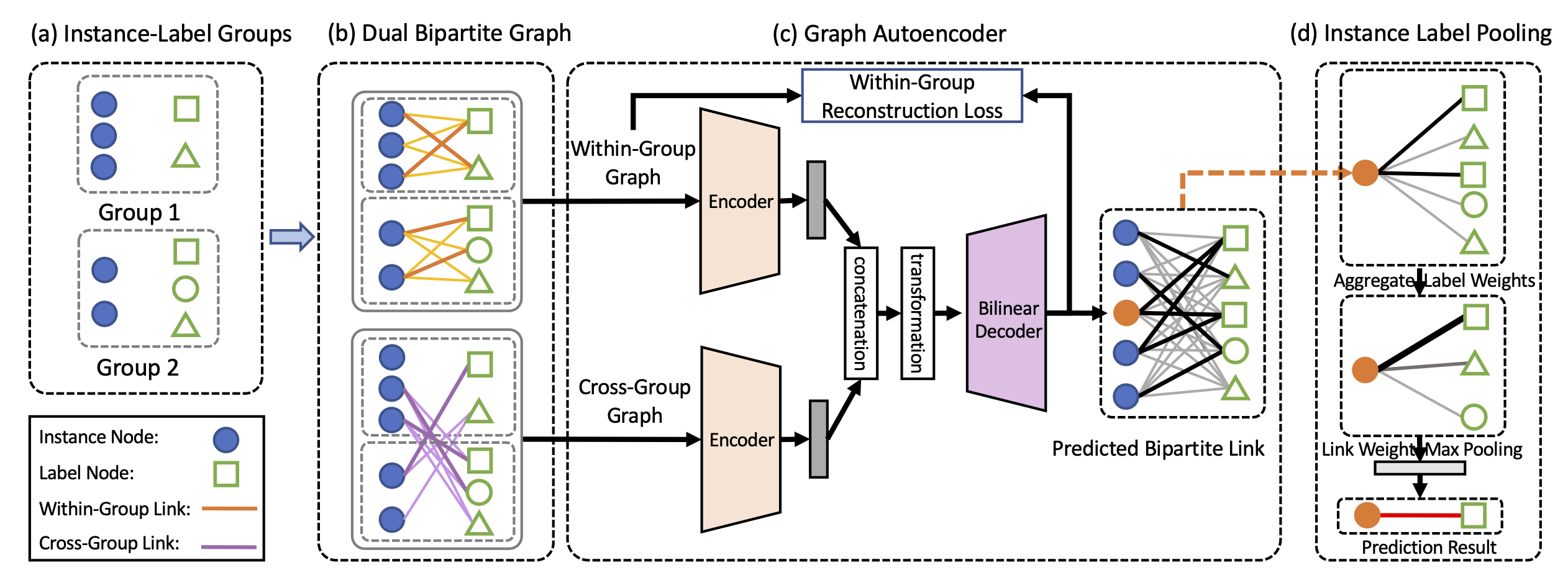
Figure 3: The framework of the proposed method can be demonstrated as four parts: (a) Problem Formulation with Instance-Label Groups. (b) Dual Bipartite Graph. (c) Graph Autoencoder. (d) Instance Label Pooling.

Related Work

Partial Label Learning (PLL) (?; ?; ?) also called superset label learning  (?) had been viewed as a weakly-supervised learning framework with implicit labeling information which assumes there is always exactly one ground-truth among the candidate label set. Therefore, one disambiguation strategy is building a certain parametric model and regarding ground-truth label as a latent variable. The model is iteratively refined by optimizing certain objectives, such as the maximum likelihood criterion (?; ?), or the maximum margin criterion (?). Another strategy assumes equal importance for all kinds of candidate labels and predicts label scores by averaging their modeling outputs  (?; ?; ?; ?; ?). Compared to the PLL problem, GPLL is much more challenging and needs to resolve group-level disambiguation, which is more general and practical for real-world scenarios.

Graph Neural Networks (GNNs) were introduced in (?; ?), and mainly focus on supervised node classification or link prediction problem based on convolutional graph networks (?; ?; ?; ?). More recently, graph autoencoder networks (?) were proposed to perform unsupervised link prediction, which we adopt for our label disambiguation problem. Unlike previous link prediction problems where the weights of observed links were given by the data. Our weights were initially estimated by clustering algorithms, which is the only information we have.

Problem Formulation

In GPLL setting, the data is provided in the form of $K$ groups $\mathcal{G}=\{g_{i}\}^{K}_{i=1}$. Each group $g_{i}$ is a collection of instances and a candidate label set where $g_{i}=\{\mathcal{X}^{(i)},\mathcal{L}^{(i)}\}$. $\mathcal{X}^{(i)}$ is the set of $M^{(i)}$ instances, $\mathcal{X}^{(i)}=\{x^{(i)}_{m}\}^{M^{(i)}}_{m=1}$, and $x^{(i)}_{m}$ is the instance feature where $x^{(i)}_{m}\in\mathbb{R}^{d}$. The associated candidate label set $\mathcal{L}^{(i)}$ is the set of $N^{(i)}$ labels, $\mathcal{L}^{(i)}=\{l^{(i)}_{n}\}^{N^{(i)}}_{n=1}$, where $l^{(i)}_{n}\in\mathcal{Y}$. The class set $\mathcal{Y}$ contains $(C+1)$ classes where $\mathcal{Y}=\{1,,...,C,null\}$, since some instances might be from background classes that never appear in the dataset labels. As shown in the GPLL examples in Introduction, the correct label for an instance in $\mathcal{X}^{(i)}$ may exist in its candidate label set $\mathcal{L}^{(i)}$ or even in another candidate label set $\mathcal{L}^{(j)}$ of another group, where $i\neq j$. The instance in $\mathcal{X}^{(i)}$ will have a $null$ label if its correct label doesn’t exist in any candidate label set $\mathcal{L}$ in $\mathcal{G}$. In a nutshell, the input of this problem is a set of groups which consist of instances and labels $\mathcal{G}=\{\mathcal{X}^{(i)},\mathcal{L}^{(i)}\}^{K}_{i=1}$. The output is the predicted label $l\in\mathcal{Y}$ for each instance $x\in\mathcal{X}$. In addition, we assume that some instances and labels repetitively co-occur across groups for the model to learn the association pattern. Moreover, the problem is naturally in a self-supervised and transductive scenario, i.e., there is no train/test split, and the data $\mathcal{G}$ is all we have for labeling the instances.

Approach

As shown in Figure 3, we describe our method for GPLL task and elaborate on each part with details: (b) In Dual Bipartite Graph, we take instances and labels as nodes and construct Within-Group or Cross-Group Link for two bipartite graphs with uncertain links. (c) We propose a Graph Autoencoder to learn the embedding representations of the bipartite graphs and iteratively refine the bipartite link weights. (d) In the final stage, we propose an Instance Label Pooling to predict the correct instance-label link for each instance.

Dual Bipartite Graph

Formally, we define our uncertain bipartite graph as $G=\{[\mathcal{X},\mathcal{L}],M\}$, $G$ is a weighted graph with instance nodes $\mathcal{X}$ and label nodes $\mathcal{L}$. $M$ denotes the uncertain links between instance $\mathcal{X}$ and label $\mathcal{L}$ with likelihood values. The likelihood of each link refers to whether a label is correct for an instance. We will construct the dual bipartite graph $M=[M^{within},M^{cross}]$ with complementary information. $M^{within}$ and $M^{cross}$ will be the edges of the Within-Group Graph and Cross-Group Graph.

Within-Group Graph Construction. As shown in Figure 3(b), we consider the second and third heuristics described in the third paragraph of the Introduction to estimate the link likelihood within a group to construct the Within-Group Graph. The within-group link weight initialization contains three steps: 1) Given a instance $x_{i}\in\mathcal{X}$ and label $l_{j}\in\mathcal{L}$, we represent the within-group link $q_{ij}$ by concatenating instance and label features to form a tuple $[x_{i};l_{j}]$. 2) We create all possible links within each of group between instances and labels and perform DBSCAN (?) to cluster the links by their link features. We choose the cluster size $c_{ij}$ for each link to describe the co-occurrence frequency of instance-label pairs. The number is the times that $x_{i}$ co-occurs with the label $l_{j}$ in the entire dataset, which assigned as the likelihood of $l_{j}$ being the correct label of $x_{i}$. 3) We will refine the likelihood by considering the contradictory relation of links within a group.We define the contradictory link for each link $q_{ij}$: the links with only one shared node (instance $x_{i}$ or label $l_{j}$) in the same group. We will refine the likelihood by dividing the total likelihood of the link $q_{ij}$ and its contradictory links. The within-group link weight is defined as follow:

$$w_{ij}=\frac{c_{ij}}{(\sum_{u\in N_{i}}c_{iu}+\sum_{v\in N_{j}}c_{vj})-c_{ij}}$$ (1)

where $N_{i}$ and $N_{j}$ are the neighbor nodes set for node $i$ and $j$. We acquire all the within-group link weights by calculating all the weights between the instances and labels within the same group and denote the weighted adjacency matrix as $M^{within}\in[0,1]^{U\times V}$ where $U$ is the number of instances in $\mathcal{X}$ and $V$ is the number of labels in $\mathcal{L}$.

Cross-Group Graph Construction. Given the within-group weights $M^{inner}$ and the first heuristic mentioned in the third paragraph of Introduction, we can initialize the cross-group link weight and construct Cross-Group Graph shown in Figure 3(b). Given an instance, we measure the l2-distance for instances and select similar instances by a certain threshold $d$ and define those nodes as homogeneous neighbor node. In addition, the homogeneous neighbors of each instance has their candidate labels, and we link the instance to these cross-group candidate labels as a cross-group link. The likelihood values of cross-group links were initialized in the previous step. We use such within-group link weight to be the likelihood between the instance and the label of its homogeneous node.

Graph Autoencoder

To predict the unknown likelihood of instance-label pairs for uncertain graph, we design a novel graph autoencoder architecture called DB-GAE. The model has the ability to 1) Encode the graph $G$ with heterogeneous within/cross-group links to a low-dimensional embedding space. 2) Dynamically update the instance-label relation while learning a new representation of the instance and label nodes. 3) Predict the link weights between instances and labels by reconstructing the observed links we initialize.

Graph Convolution Encoder. Given the node features $[\mathcal{X},\mathcal{L}]$ and the link weights $[M^{within},M^{cross}]$ initialized in the previous step, we aim to encode such information in node representation for further prediction. The graph convolution model incorporates the neighbor information by propagating the message to form a new representation of a node. We utilized this characteristic to use the link information during propagation to obtain a more representative embedding. For expressing the propagation of within-group links, a single hidden layer GCN is given by

$$\boldsymbol{H}^{i}=f(\boldsymbol{H}^{i-1},M^{within})$$ (2)

where $\boldsymbol{H}^{0}=[\mathcal{X},\mathcal{L}]$ and $f$ is a propagation rule. Each layer $\boldsymbol{H}^{i}$ corresponds to the instance and label feature matrix $[\mathcal{X},\mathcal{L}]$ and where each row is a feature representation of a node. This operation is similar to a filtering operation in the CNN  (?), and the features become increasingly more abstract at each consecutive layer. We aggregate the feature representation of each node by its associated neighbors. Moreover, the neighbors were weighted by the within-group weight $w_{ij}$ and transformed by applying the weights $W$ before propagation. To avoid the interference between within-group and cross-group link propagation, we have distinct propagation rules of dual bipartite GCNs for within-group links and cross-group links separately. The propagation rule for within-group and cross-group can be denoted as:

$$\mu_{j\rightarrow i}=w_{ij}Wl_{j}\quad\mu_{j^{\prime}\rightarrow i}=w_{ij^{\prime}}Wl_{j^{\prime}}$$ (3)

where the $w_{ij}$ and $w_{ij^{\prime}}$ are link weights computed from the previous section and $j^{\prime}$ is a cross-group label. $W$ is a learnable parameter. This operation is similar to the spectral rule propagation (?) where the propagation is normalized based on the degree of both $i$ and $j$. Instead, our propagation is normalized by the link weight of both $i$ and $j$. We aggregate incoming messages for each of instance from label nodes by accumulating all neighbors $N_{i}$ to represent the node, denoted as:

$$h_{i}^{within}=\sigma(\sum_{j\in N_{i}}\mu_{j\rightarrow i})\quad h_{i}^{cross}=\sigma(\sum_{j^{\prime}\in N_{i}}\mu_{j^{\prime}\rightarrow i})$$ (4)

$h_{i}^{within}$ is the hidden vector that represents the instance node $i$ by within-group and $h_{i}^{cross}$ is the hidden vector that represents the instance node $i$ by cross-group. To arrive at the final embedding of instance node $i$ and label node $j$, we apply the concatenate operation over the hidden vector updated from the within-group and cross-group. The model has a non-linear transformation to transform the concatenated representations for each node by dual path GCN to a unified embedding representation. After concatenation, the feature will feed into a dense layer to obtain the final representation, denoted as:

$$u_{i}=\sigma(W_{u}[h_{i}^{within};h_{i}^{cross};f_{i}])$$ (5)

$$v_{j}=\sigma(W_{v}[h_{j}^{within};h_{j}^{cross};n_{j}])$$ (6)

$\sigma(\cdot)$ denotes an ReLU activation function. $W_{u}$ and $W_{v}$ are learnable parameters. We use the transformation functions of $f_{i}=\sigma(W_{f}x_{i}+b)$ and $n_{j}=\sigma(W_{n}l_{j}+b)$ in our paper. The output of the encoder will be the updated representations $[\boldsymbol{U,V}]$ for the instances and labels.

Graph Attention for Within/Cross-Group Propagation. The graph convolution is based on the probability value of in the dual bipartite graph, which is fixed during the graph propagation process. Moreover, we want to continuously update the representations of nodes to predict the link weights by learning from links with uncertainty. Hence, dynamically adjust the propagation weight between instances and labels by considering the features itself is essential. To this end, we can employ some form of attention mechanism (?) which actively learn how to propagate the information to optimize our result. To perform the attention on nodes, attention coefficients can be calculated by:

$$e_{ij}=a(W_{a}x_{i},W_{a}l_{j})$$ (7)

It indicates the importance of label node $l_{j}$’s features to instance node $x_{i}$, and $W_{a}$ is its learnable weight matrix, and $a$ is a feed-forward network. We inject the graph structure into the mechanism by performing masked attention which means we compute $\alpha_{ij}$ for nodes $j\in N_{i}$, where $N_{i}$ is the neighbor nodes of node $i$ in the graph. To make coefficients easily comparable across different nodes, we normalize them across all choices of $j$ using the softmax function:

$$\alpha_{ij}=\frac{exp(e_{ij})}{\sum_{k\in N_{i}}exp(e_{ik})}$$ (8)

We learn two kinds of link information by graph attention, including the within-group link weight and cross-group link weight. Therefore, the propagation rule in Equation 3 can be extended to:

$$\mu_{j\rightarrow i}=\alpha_{ij}w_{ij}Wl_{j}\quad\mu_{j^{\prime}\rightarrow i}=\alpha_{ij^{\prime}}w_{ij^{\prime}}Wl_{j^{\prime}}$$ (9)

where $\alpha$ is the context vector which represents the normalized contribution of label $j$ to instance $i$. After aggregating the information though the neighbors by summation and apply averaging on the $K$ transformation attention by multi-head attention (?), the Equation 4 becomes:

$$h^{within}_{i}=\sigma(\frac{1}{K}\sum_{k=1}^{K}\ \sum_{j\in N_{i}}\mu^{k}_{j\rightarrow i})$$ (10)

$$h^{cross}_{i}=\sigma(\frac{1}{K}\sum_{k=1}^{K}\ \sum_{j^{\prime}\in N_{i}}\mu^{k}_{j^{\prime}\rightarrow i})$$ (11)

Bi-linear Decoder for Link Resolution. To predict the link values between instances and labels, we decode the updated embedding that contains the within-group, cross group, and feature information. In addition, we can use Bi-linear decoder model (?) to reconstruct links of the bipartite graph by considering the node feature similarity. The reconstruction model is $M=\sigma(\boldsymbol{U}^{T}\boldsymbol{V})$, and likelihood between instance $i$ and label $j$ is $\hat{M}_{ij}$. The learning objective is to reconstruct the weights of the observed links (estimated from the within-group initialization) and predict the weights of unobserved links (cross-group link). The score function of the decoder is:

$$p(\hat{M}_{ij}=r)=\frac{e^{u^{T}_{i}Q_{r}v_{j}}}{\Sigma_{s\in R}e^{u^{T}_{i}Q_{s}v_{j}}},$$ (12)

where $Q_{r}$ is the trainable parameter matrix of shape $E\times E$, and $E$ is the dimension of hidden representations. $r$ is weighting scale from 0 to 1 which represents the likelihood of the link. The predicted rating is computed as:

$$\hat{M}_{ij}=g(u_{i},v_{j})=\mathbb{E}_{p(\hat{M}_{ij}=r)}[r]=\sum_{r\in R}rp(\hat{M}_{ij}=r)$$ (13)

Within Group Reconstruction Loss. To optimize the proposed graph inference networks, we follow the loss function defined in (?) to minimize the reconstruction loss by negative log likelihood of the predicted likelihood:

$$\mathcal{L}=-\sum_{i,j;\Omega_{ij}=1}\sum_{r=1}^{R}I[r=M^{within}_{ij}]\log p(\hat{M}_{ij}=r),$$ (14)

where the matrix $\Omega\in{0,1}$ is a mask for unobserved links in the within-group matrix $M^{within}$. We optimize over the observed links to predict the likelihood of the matrix $\hat{M}$ which contains observed links and unobserved links.

Link Prediction by Instance Label Pooling

To infer the label of each instance, we use the predicted link weight $\hat{M}_{ij}$ generated by DB-GAE. As shown in Figure3(d), given an instance, we aggregate all the weights of the links it connects by different classes. For within-group link weight, we directly use the predicted link weight. For cross-group link weight, we multiply the predicted link weight with the cosine similarity of the instance $i$’s feature and its homogeneous neighbor’s feature. That is because the link weight should be lower if the feature similarity is low. The weight of a class $o$ being the label of instance $i$ is calculated by:

$$W_{o}^{i}=\sum_{j\in o;\Omega_{ij}=1}\sigma(\hat{M}_{ij})+\sum_{j\in o;\Omega^{\prime}_{ij^{\prime}}=1}\sigma(\hat{M}_{ij^{\prime}}\frac{f_{i}\cdot f_{i^{\prime}}}{||f_{i}||||f_{i^{\prime}}||})$$ (15)

where the $\sigma$ represents a ReLU over a sigmoid function. $\Omega^{\prime}\in{0,1}$ is a mask for unobserved links in the cross group matrix $M^{cross}$. We aggregate the link weight by the same class and pool the class with the maximum weighted score $p_{i}=argmax_{o\in\mathcal{Y}}(W^{i}_{o})$ as the predicted label of instance $x_{i}$. If the score is equal to 0, it means there is no prediction, we predict it as a $null$.

General Partial Label Learning Datasets

We evaluate the performance of our model for the automatic face naming problem on two real-world datasets: MPII-MD (?) and M-VAD (?). MPII-MD dataset in GPLL setting, which contains only group-level supervision with cross group labels and $null$ labels. The M-VAD dataset is constructed for PLL setting, which has less ambiguity but larger-scale data.

MPII-MD: MPII Movie Description Dataset. The MPII-MD dataset consists of face images and ambiguous labels automatically extracted using the screenplays provided in 13 movies with 806 different faces and 181 possible names from 558 image-caption pairs. We select the frames from the data with detectable faces and corresponding captions. The percentage of the faces with a $null$ label in the dataset are 21%.

M-VAD: Montreal Video Annotation Dataset. In M-VAD Names dataset contains fully annotated faces in images with names in the captions from 55 movies. It consists of 222,58 detected faces and 591 possible names from 17,533 image-caption pairs.

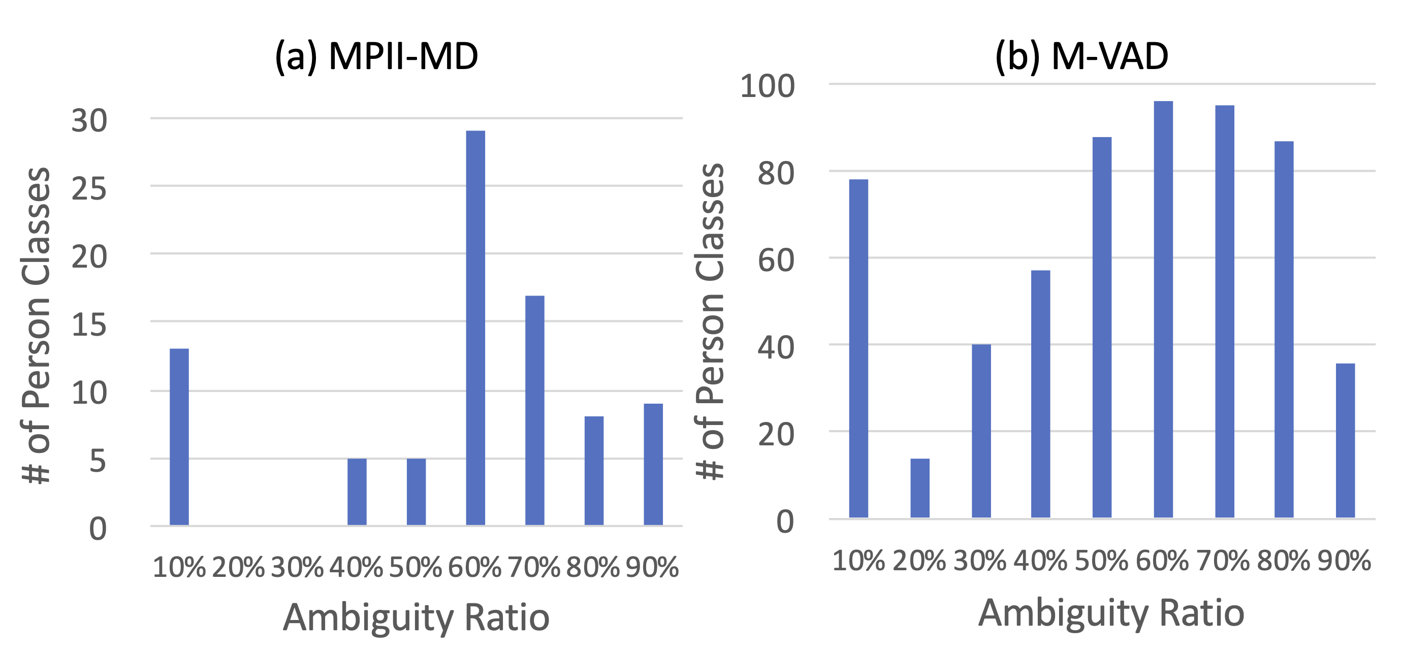
Figure 4: Data Distribution over Ambiguity Ratio

Data Distribution over Ambiguity Ratio. To explore the data difficulty of the datasets, we define ambiguity ratio and show the histogram over different levels of ambiguity, as shown in Figure 4. The metric refers to a fraction of all possible instance-label links that are incorrect, the ambiguity ratio of a label with class $c\in\mathcal{Y}$ is defined by:

$$\mathcal{R}_{o}=1-\frac{\sum_{i=1}^{K}|s^{(i)}_{t}|}{\sum_{i=1}^{K}|s^{(i)}_{t}|+|s^{(i)}_{f}|}$$ (16)

where $i$ is the group index. $s_{t}^{(i)}$ is the set of correct instance-label links in the group $g^{(i)}$ with class $o$. $s_{f}^{(i)}$ is the set of wrong links in group $g^{(i)}$ which connect to instance node or label node with class $o$.

Table 1: Performance Comparison on MPII-MD and M-VAD

	MPII-MD		M-VAD
Method	F1-score	Accuracy	Accuracy
Pair Clustering	0.539	45.0 %	78.2 %
Cluster Voting	0.558	46.5 %	78.9 %
SURE	0.605	48.7 %	85.7 %
IPAL	0.608	48.3 %	86.1 %
PL-LEAF	0.610	48.6 %	86.3 %
PL-AGGD	0.598	47.6 %	86.5 %
Our method	0.768	76.5 %	90.3 %

Baselines

Cluster Voting (?): For each instance, the method selects candidate labels from the same cluster. The correct label is determined by majority voting over all the candidates. To cluster faces by visual features for face naming datasets, we apply DBSCAN (with $\epsilon=1,n=2$).

Pair Clustering (?): As in the Within-Group Graph Construction, we perform pair clustering to estimate the likelihood of a link. Given an instance, we find its link with the largest cluster size and pick its label as the prediction, We also perform DBSCAN (with $\epsilon=1,n=2$) for pair clustering.

IPAL (?): IPAL is an instance-based PLL model and disambiguates candidate labels by an iterative label propagation procedure.

PL-LEAF (?): PL-LEAF is a feature-aware approach which learns the manifold structure of feature space and performs regularized multi-output regression over the generated labeling confidences.

SURE (?): SURE proposes a unified formulation with the maximum infinity norm regularization to train the desired model and perform pseudo-labeling jointly.

PL-AGGD (?): PL-AGGD proposes a unified framework which jointly optimizes the ground-truth labeling confidences, similarity graph, and model parameters to achieve generalization performance.

Experimental Setup

For all runs, we use pre-trained FaceNet (?) to extract the visual embedding for detected faces with 512 dimensions from the images and apply a threshold $d=1$ suggested in the paper (?) for $l_{2}$ distance to determine two faces are the same person. We encode names using one-hot vectors. In DB-GAE, we use the Adam optimizer (?) with a learning rate of 0.001. The layer sizes of graph convolution (with ReLU) is 1000 and 100 for the dense layer. We run 1000 epochs on both datasets with the runtime of 10min on MPII-MD dataset and 5hr 10min on the M-VAD dataset on CPU. Since M-VAD dataset has sufficient training data, we perform 10-fold cross-validation on the partial label learning method with 9:1 train/test split. For our method, we only use the same testing data (10% data) because our method does not require additional training data. More details of the model architecture, parameter list, and analysis of the time complexity of the model will be included in the arXiv version.

Methods Performance Comparison

From Table 1, our proposed method outperforms the baselines in both datasets with a significant margin by 0.158 absolute improvements of F1-score for GPLL dataset and 3.8% absolute improvement of accuracy in PLL dataset. In the experimental results on MPII-MD dataset, the best baseline reach about 0.61 on F1-score and 49% on accuracy, and proposed model can achieve the best performance with over 0.76 on F1-score and 73% on accuracy. The significant improvements show that our model is powerful enough to deal with generalized ambiguity, and the baseline methods will fail to disambiguate distractors. As shown in the results on M-VAD dataset, PLL methods performed much better when using sufficient training data for PLL setting. Our model is able to achieve the best performance among the methods with only one-tenth of data in the transductive setting. This result shows its ability to resolve the extreme ambiguity caused by data sparsity.

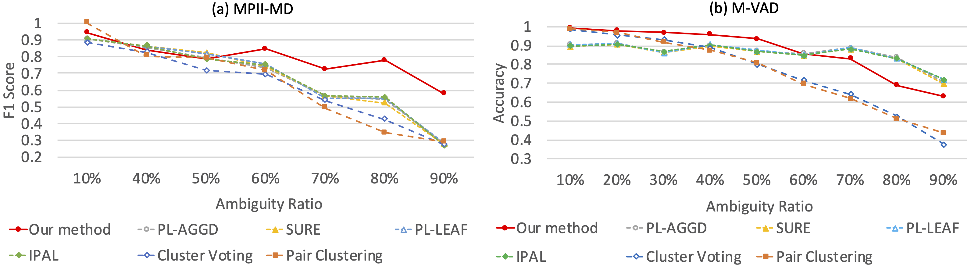
Figure 5: F1-score and accuracy curves versus ambiguity ratios on MPII-MD and M-VAD.

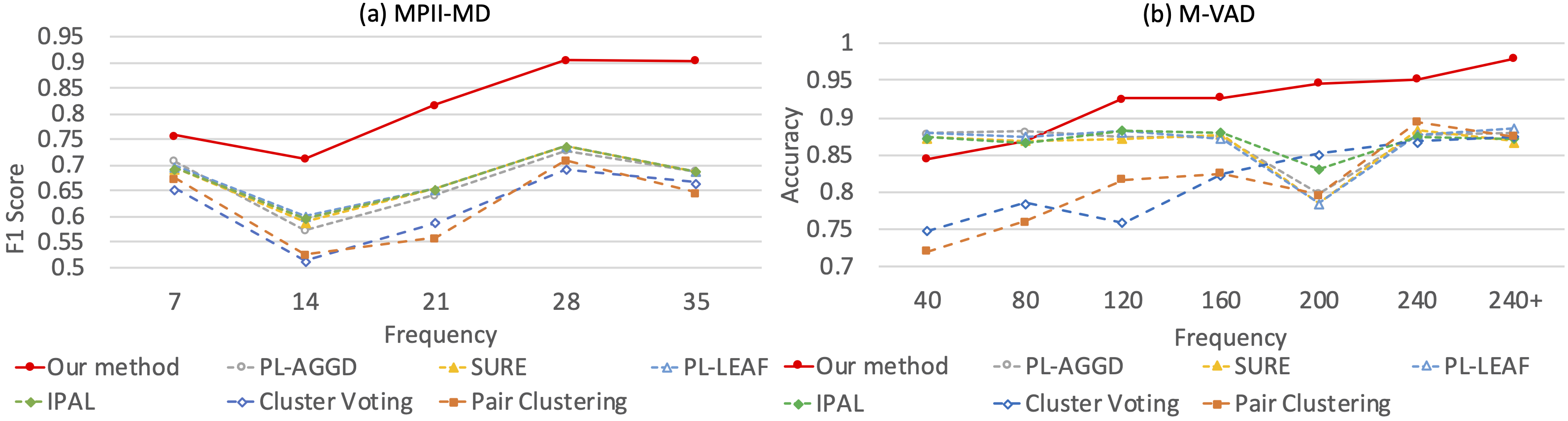
Figure 6: F1-score and accuracy curves versus ground-truth frequency on MPII-MD and M-VAD.

Condition Controlled Experiments

In addition to overall performance results, we show the comparison with baselines for different levels of data difficulty.

The effect of ambiguity ratio on performance. In the Figure 5(a), the baselines can reach comparable performances with the proposed model when the ambiguity is not severe (ambiguity ratio $<$ 0.4). Their performances will drop a lot when they meet high levels of data ambiguity (ambiguity ratio $>$ 0.4). In less ambiguity dataset (PLL setting) Figure 5(b), we can see that the proposed method is comparable with the state-of-the-art PPL method without addtional training data.

The effect of ground-truth frequency on performance. The ground-truth frequency is the number of face-name pairs with the same class co-occur in the same group throughout the dataset. In Figure 6 (a), we can see that our model performs better than other methods in general. Almost all of the methods exhibit a slight drop in the ground-truth frequency of $14$, because the average ambiguity ratio at frequency interval is higher than the middle ambiguity ratio of frequency $7$. In Figure 6(b), the approach performs better than other methods. The accuracy of the model will continually increase even beyond 95% if the correct face-name co-occur frequently enough.

Table 2: Ablation Study of Proposed Method DB-GAE

	MPII-MD		M-VAD
Method	F1-score	Accuracy	Accuracy
DB-GAE	0.768	76.5%	90.3%
w/o Graph Autoencoder	0.614	62.9%	81.6%
w/o Dual Bipartite Graph	0.724	68.4 %	88.3 %
w/o Cross-Group Link	0.730	73.9 %	89.2 %
w/o Graph Attention	0.743	76.4 %	87.3 %

Ablation Study

To reveal the contribution of each component, we test the performance of DB-GAE by removing different parts: Graph Autoencoder, Dual Bipartite Graph Architecture (apply GAE and set all weights for instance label links to be averaged (?; ?)), Cross-Group Link, and Graph Attention. The comparison results of ablation study are shown in the Table 2, we can see that the Graph Autoencoder contributes the most of performance improvement. The GAE (w/o Dual Bipartite Graph Architecture) encounters an accuracy drop in the MPII-MD dataset because it is unable to deal with null distractors since the weights fed into the GAE are all links with a high likelihood. The consideration of Cross-Group Link will help the model to deal with the group-level ambiguity. The F1-score of DB-GAE (w/o Cross-Group Link) drops obviously on MPII-MD. The improvement of DB-GAE over DB-GAE (w/o Graph Attention) verifies our hypothesis that graph attention can help to capture a better representation of the graph structure.

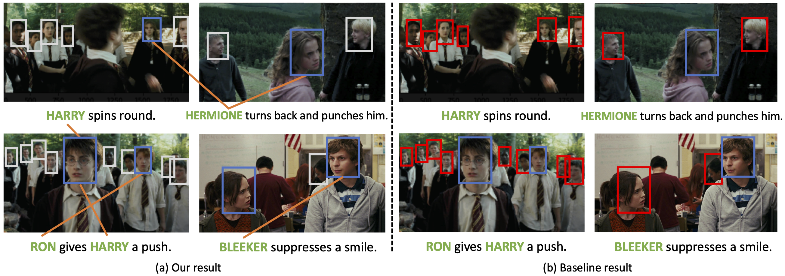
Figure 7: Qualitative examples from MPII-MD dataset. The blue/grey box represents the correct prediction of a name/null label. Red box represents the wrong prediction. The orange line visualize the predicted link between face and name.

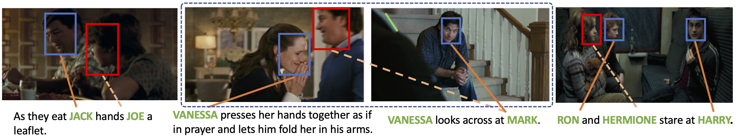
Figure 8: Failure cases from MPII-MD dataset. The dashed line represents the ground-truth link between face and name which the model misses.

Qualitative Results

As shown in Figure 7, compared to the best baseline: PL-LEAF in our MPII-MD experiment, our model can correctly predict the $null$ labels and cross-group labels even when the number of distractors is large within a group. Also, the performance for within-group label prediction is also better since the model incorporates cross-group knowledge to resolve the within-group ambiguity.

Failure Cases

From Figure 8, we can conclude that 1) The visual recognition rate may affect the within-group linking performance. In the first example, didn’t link to , which was limited by the feature representation. 2) Also, it will affect the cross-group linking due to the failure of finding similar faces. should link to the name to find its correct label but the model can’t find as similar faces. 3) The current model is based on correlation and thus lacks reasoning ability, for example, we humans may rule out other faces and predict the correct link, but our method fails. For example, when predicting , since we know and were linked, we can infer is more likely to be .

Conclusions

We introduced the General Partial Label Learning (GPLL) problem, which is more realistic and general than the traditional PLL. The proposed approach DB-GAE was designed to tackle the challenges of GPLL by disambiguating the within-/cross-group instance-label links with richer contextual graph representations. We contributed two GPLL benchmarks on automatic face naming tasks. We found that DB-GAE outperformed the best baseline with absolute 0.159 F1-score and 24.8% accuracy. Further analysis shows the robustness of DB-GAE in generalized ambiguity scenarios and the effect of various ambiguity levels. Moving forward, we are going to frame more tasks into GPLL such as cross-domain co-reference resolution in NLP, and push the envelope of DB-GAE in other fields.

References

- [Berg, Kipf, and Welling 2017] Berg, R. v. d.; Kipf, T. N.; and Welling, M. 2017. Graph convolutional matrix completion. arXiv preprint arXiv:1706.02263.
- [Cour, Sapp, and Taskar 2011] Cour, T.; Sapp, B.; and Taskar, B. 2011. Learning from partial labels. Journal of Machine Learning Research 12(May):1501–1536.
- [Defferrard, Bresson, and Vandergheynst 2016] Defferrard, M.; Bresson, X.; and Vandergheynst, P. 2016. Convolutional neural networks on graphs with fast localized spectral filtering. In Advances in neural information processing systems, 3844–3852.
- [Feng and An 2019] Feng, L., and An, B. 2019. Partial label learning with self-guided retraining. arXiv preprint arXiv:1902.03045.
- [Gong et al. 2017] Gong, C.; Liu, T.; Tang, Y.; Yang, J.; Yang, J.; and Tao, D. 2017. A regularization approach for instance-based superset label learning. IEEE transactions on cybernetics 48(3):967–978.
- [Gori, Monfardini, and Scarselli 2005] Gori, M.; Monfardini, G.; and Scarselli, F. 2005. A new model for learning in graph domains. In Proceeding of 2005 IEEE International Joint Conference on Neural Networks, 2005., volume 2, 729–734. IEEE.
- [Huang, Gao, and Zhou 2018] Huang, S.-J.; Gao, W.; and Zhou, Z.-H. 2018. Fast multi-instance multi-label learning. IEEE transactions on pattern analysis and machine intelligence.
- [Hüllermeier and Beringer 2006] Hüllermeier, E., and Beringer, J. 2006. Learning from ambiguously labeled examples. Intelligent Data Analysis 10(5):419–439.
- [Kingma and Ba 2014] Kingma, D. P., and Ba, J. 2014. Adam: A method for stochastic optimization. arXiv preprint arXiv:1412.6980.
- [Kipf and Welling 2016a] Kipf, T. N., and Welling, M. 2016a. Semi-supervised classification with graph convolutional networks. arXiv preprint arXiv:1609.02907.
- [Kipf and Welling 2016b] Kipf, T. N., and Welling, M. 2016b. Variational graph auto-encoders. arXiv preprint arXiv:1611.07308.
- [Kiros, Salakhutdinov, and Zemel 2014] Kiros, R.; Salakhutdinov, R.; and Zemel, R. S. 2014. Unifying visual-semantic embeddings with multimodal neural language models. arXiv preprint arXiv:1411.2539.
- [Kupfer and Zorn 2019] Kupfer, A., and Zorn, J. 2019. Valuable information in early sales proxies: The use of google search ranks in portfolio optimization. Journal of Forecasting 38(1):1–10.
- [LeCun, Bengio, and others 1995] LeCun, Y.; Bengio, Y.; et al. 1995. Convolutional networks for images, speech, and time series. The handbook of brain theory and neural networks 3361(10):1995.
- [Liu and Dietterich 2014] Liu, L., and Dietterich, T. 2014. Learnability of the superset label learning problem. In International Conference on Machine Learning, 1629–1637.
- [Nguyen and Caruana 2008] Nguyen, N., and Caruana, R. 2008. Classification with partial labels. In Proceedings of the 14th ACM SIGKDD international conference on Knowledge discovery and data mining, 551–559. ACM.
- [Pini et al. 2019] Pini, S.; Cornia, M.; Bolelli, F.; Baraldi, L.; and Cucchiara, R. 2019. M-vad names: a dataset for video captioning with naming. Multimedia Tools and Applications 78(10):14007–14027.
- [Rohrbach et al. 2017] Rohrbach, A.; Rohrbach, M.; Tang, S.; Oh, S. J.; and Schiele, B. 2017. Generating descriptions with grounded and co-referenced people. In 30th IEEE Conference on Computer Vision and Pattern Recognition (CVPR 2017).
- [Sander et al. 1998] Sander, J.; Ester, M.; Kriegel, H.-P.; and Xu, X. 1998. Density-based clustering in spatial databases: The algorithm gdbscan and its applications. Data mining and knowledge discovery 2(2):169–194.
- [Scarselli et al. 2008] Scarselli, F.; Gori, M.; Tsoi, A. C.; Hagenbuchner, M.; and Monfardini, G. 2008. The graph neural network model. IEEE Transactions on Neural Networks 20(1):61–80.
- [Schroff, Kalenichenko, and Philbin 2015] Schroff, F.; Kalenichenko, D.; and Philbin, J. 2015. Facenet: A unified embedding for face recognition and clustering. In Proceedings of the IEEE conference on computer vision and pattern recognition, 815–823.
- [Tang and Zhang 2017] Tang, C.-Z., and Zhang, M.-L. 2017. Confidence-rated discriminative partial label learning. In Thirty-First AAAI Conference on Artificial Intelligence.
- [Veličković et al. 2017] Veličković, P.; Cucurull, G.; Casanova, A.; Romero, A.; Lio, P.; and Bengio, Y. 2017. Graph attention networks. arXiv preprint arXiv:1710.10903.
- [Wang, Li, and Zhang 2019] Wang, D.-B.; Li, L.; and Zhang, M.-L. 2019. Adaptive graph guided disambiguation for partial label learning. In Proceedings of the 25th ACM SIGKDD International Conference on Knowledge Discovery & Data Mining, 83–91. ACM.
- [Wu and Zhang 2018] Wu, X., and Zhang, M.-L. 2018. Towards enabling binary decomposition for partial label learning. In IJCAI, 2868–2874.
- [Wu et al. 2015] Wu, J.; Yu, Y.; Huang, C.; and Yu, K. 2015. Deep multiple instance learning for image classification and auto-annotation. In Proceedings of the IEEE Conference on Computer Vision and Pattern Recognition, 3460–3469.
- [Xie and Huang 2018] Xie, M.-K., and Huang, S.-J. 2018. Partial multi-label learning. In Thirty-Second AAAI Conference on Artificial Intelligence.
- [Xu, Lv, and Geng 2019] Xu, N.; Lv, J.; and Geng, X. 2019. Partial label learning via label enhancement. In AAAI Conference on Artificial Intelligence.
- [Yu and Zhang 2016] Yu, F., and Zhang, M.-L. 2016. Maximum margin partial label learning. In Asian Conference on Machine Learning, 96–111.
- [Zhang and Chen 2018] Zhang, M., and Chen, Y. 2018. Link prediction based on graph neural networks. In Advances in Neural Information Processing Systems, 5165–5175.
- [Zhang and Yu 2015] Zhang, M.-L., and Yu, F. 2015. Solving the partial label learning problem: An instance-based approach. In Twenty-Fourth International Joint Conference on Artificial Intelligence.
- [Zhang, Zhou, and Liu 2016] Zhang, M.-L.; Zhou, B.-B.; and Liu, X.-Y. 2016. Partial label learning via feature-aware disambiguation. In Proceedings of the 22nd ACM SIGKDD International Conference on Knowledge Discovery and Data Mining, 1335–1344. ACM.
- [Zitnik and Leskovec 2017] Zitnik, M., and Leskovec, J. 2017. Predicting multicellular function through multi-layer tissue networks. Bioinformatics 33(14):i190–i198.