One-Shot Coordination of First and Last Mode Transportation

Abstract

In this paper, we consider coordinated control of feeder vehicles for first and last mode transportation. The model is macroscopic with volumes of demands and supplies along with flows of vehicles. We propose a one-shot problem for transportation of demand to or from a hub within a fixed time window, assuming the knowledge of the demand and supply configurations. We present a unified optimization framework that is applicable for both operator profit maximization and social welfare maximization. The latter goal is useful for applications such as disaster response. The decision variables in the optimization problem are routing and allocations of the vehicles for different services.

With K.K.T. analysis we propose an offline method for reducing the problem size. Further, we also analyze the problem of maximizing profits by optimally locating the supply for a given total supply and present a closed form expression of the maximum profits that can be earned over all supply configurations for a given demand configuration. We also show an equivalence between optimal supply location in the first mode problem and the last mode problem. We present a model for pricing based on the cost and travel time of the best alternate transportation and present necessary conditions for the feeder service to be viable. We illustrate the results through simulations and also compare the proposed model with a traditional vehicle routing problem. Through simulations, we also compare with the microscopic version of the problem with the decision variables being integers. We demonstrate that the route reduction algorithm proposed for the macroscopic formulation is still useful for computing nearly optimal solutions to the microscopic problem with much improved computational efficiency.

I Introduction

This paper explores the idea of a coordinated and demand responsive feeder service with a single origin (destination) and multi destination (origin) setup, over a hard single time-window. This problem occurs in scenarios such as evacuation and distribution of relief materials in response to disasters [2] and transportation for one-time events with a large foot-fall. Furthermore, this scenario has potential applications in multi-modal transportation systems where the main mode follows a schedule and needs to be coordinated with first and last modes to achieve a coordinated system. This potential application is seen in many cases like peak-hour single destination para-transit [3], freight transportation [4], express courier systems [5] etc.

Literature Review

In the context of routing of transportation services, the vehicle routing problem (V.R.P.) [6, 7, 8, 9, 10] assumes a depot from where one or more vehicles are routed via locations where one or more types of entities are picked up at their origin(s) and dropped off at their destination(s). There are also many variations to the basic V.R.P. like capacitated [8], multiple origin and destination [7], multiple time window [9, 7] or simultaneous pick-up and delivery [6] etc. Sharing some similarities with V.R.P. are the ride sharing problem [11, 12, 13, 14] and dial-a-ride problem [15, 16, 17]. In these problems, the aim is to match vehicles with the passengers while maximizing operator’s profits in some time windows. Recently, there has also been a growing interest in routing problems with awareness of the demand and the fleet. For example,  [18, 19] explore the problem of optimally dispatching taxis based on the location of the taxis and customer requests.

While many routing problems deal with discrete vehicles and discrete entities to be transported, macroscopic models that deal with flows of vehicles and volumes of demand and supply are also common. Though less realistic than discrete models, they allow for computationally easier solutions and greater scope for analysis and higher order planning. In the context of demand anticipative mobility, [20, 21, 22, 23, 24] aim to match demand and supply by routing autonomous vehicle flows and maximize throughput in the network through a steady-state design of the load-balancing and routing flow rates. Much of the literature on fleet routing is in the context of uni-modal or single hop transportation services. Though multi-modal transportation has been extensively studied, dynamic, demand and supply aware first and last mode service is not sufficiently studied [25].

There have been multiple studies on humanitarian aid planning. Evacuation and distribution of relief material in disaster management scenarios form the prime focus of such studies [26, 27, 28, 29]. Most of these studies focus on determining the location of the ware-houses and safe-houses given the forecasts. [30] proposes a multi-depot location-routing problem (MDLRP). The MDLRP considers network failure with multiple use of vehicles, and a standard relief time. [31] analyzes a last-mile delivery problem to gain insights into the underlying route structures and provide observations on routing aspects that are necessary for planning out disaster relief operations. The results are in the context of three scenarios: time minimization, demand maximization and service comparability. [32] proposes a multi-criterion last-mile routing problem, while [33] considers a capacitated routing problem which minimizes the maximum response time for relief to reach the affected regions. In [34], a time-windowed V.R.P. with a single depot is proposed for the purpose of humanitarian aid distribution.

Contributions

In this paper, we consider the first-mode or feed-in problem and the last-mode or feed-out problem, wherein all the demand has a common destination and origin, respectively. The following are the main contributions of this paper.

• Model: We present a macroscopic network flow model for the one-shot feed-in and feed-out problems. We call it “one-shot” since there is a single hard time window within which the transportation has to occur. Given the demand and supply configuration on a network, the optimization problem determines optimal routing of the vehicles and servicing of the demand. We also consider the combined problem of optimal supply location and routing. The proposed model includes both maximization of monetary profit and maximization of serviced demand or social welfare as special cases, depending on the choice of the parameters.

• Analysis and algorithm: We carry out a rigorous mathematical analysis of the optimization problem, based on which we propose an offline algorithm to reduce the problem size by pruning “non-profitable” routes and decision variables. We also analyze the feed-in and feed-out settings, following which we establish an equivalence between the optimal supply location problems in the two settings. We also present an analysis of the maximum possible profits.

• Viability analysis: We propose a priority-based pricing model that is general enough to be applicable for monetary profit maximization as well as social welfare maximization. We carry out mathematical analysis on the parameters to come up with necessary conditions for the viability of the feeder service and for routes with multiple trips to a hub node to be chosen in an optimal solution. Such analysis is useful for higher level planning.

• Simulations: We present a collection of simulations on multiple graphs that validate our analytical results. These simulation results include a realistic scenario of pre-positioning of relief material anticipating the devastation caused by a cyclone. We construct the graph and various other parameters in this simulation based on data from Odisha, a state in India that is prone to severe cyclones.

• Comparisons with microscopic problem: Through simulations, we also compare the macroscopic problem with the microscopic problem, wherein the demands, supplies and service pick-ups are all integers. We show that the macroscopic problem gives very good bounds on the optimal objective value for the microscopic problem. Moreover, the solution to the microscopic problem on the reduced route set, obtained from the proposed macroscopic analysis, is shown to be only slightly suboptimal compared to the solution of the microscopic problem on the original complete route set. The computational effort required to solve the microscopic problem on the reduced route set is significantly lesser compared to the effort required to solve the microscopic problem on the complete route set. Thus, the analysis on the macroscopic problem, and the resulting route reduction algorithm is very useful even for solving the more realistic microscopic problem.

On the modeling front, demand anticipative mobility problem in [20, 21, 22, 23, 24] though is for a macroscopic network flow model, it is concerned with designing steady state flows whereas we consider routing in a fixed hard time window. Similarly, ride sharing and taxi dispatch do not address fixed horizon planning necessary for single events, such as in disaster relief. Compared to the problems on disaster relief [30, 31, 32, 33, 34], we present a unified model that is applicable for both disaster response as well as non-humanitarian applications such as transportation for large public events. Our model can also incorporate priorities for demand at different nodes, depending on say the local severity of a disaster.

Compared to the V.R.P. literature in general, including the papers on disaster relief, we start with a macroscopic formulation and carry out rigorous mathematical analysis on the optimal solutions. The resulting route reduction algorithm and the demonstration of its computational efficiency in solving even the microscopic problem is unique, to the best of our knowledge. Similarly, the kind of viability analysis that we do is typically missing in the V.R.P. and network flow literature.

In the preliminary version [1] of this paper, we considered only the feed-in problem and supply location problem. Here, we additionally provide results for the feed-out problem and introduce a model for carrying out the analysis on the viability of the feeder service. Moreover, here we also provide the proofs missing in [1]. We also have an expanded simulation section where we compare the macroscopic and microscopic versions of the problem. Furthermore, we present a realistic application of planning the relief distribution post a cyclone.

Organization

The rest of the paper is organized as follows - we set up the one-shot problem in Section II. In Section III we describe the properties of its optimal solutions and the off-line route-set reduction method. We present the priority-based pricing model in Section IV. In Section V, we discuss the supply location problem and analyze maximum possible profits with a given total supply for a given demand configuration. We also show the equivalence with the supply optimized feed-out in this section. We present the simulation results in Section VI and provide concluding remarks in Section VII. We present the proofs of all but the main theorems in appendices.

Notation

We use ${\mathbb{Z}}$, ${\mathbb{N}}$ and ${\mathbb{N}}_{0}$ for the set of integers, natural numbers and ${\mathbb{N}}\cup\{0\}$, respectively. We use $[a,b]_{\mathbb{Z}}$ and $(a,b]_{\mathbb{Z}}$ to denote $[a,b]\operatorname{\cap}{\mathbb{Z}}$ and $(a,b]\operatorname{\cap}{\mathbb{Z}}$, respectively.

II Problem Setup

In this section, we setup the coordinated first and last mode transportation problem using a macroscopic formulation. Since this is a network-flow problem, we first present a graph model, and then define the route sets used for optimization. Finally, we present the optimization model.

II-A Network Setup

We assume that the operator wants to provide service in a region of interest, which we model as a graph $G:=(V,E)$, where $V$ is the set of nodes and $E$ is the set of edges between the nodes. Here, each node $l\in V$ represents an area within the region of interest. For both the feed-in and feed-out problems we have a special node, which we call as the hub, denoted by $H$. In the case of a feed-in problem we have a demand flow from the areas of the region directed to the hub $H$, while the opposite happens for the feed-out problem. Thus, in both these problems, we assume that for each node $l$ there is a demand $d_{l}\geq 0$ that needs to be serviced. This is either spatially distributed in the region for the feed-in problem, or is concentrated at the hub $H$ for the feed-out problem. Furthermore, we assume that the operator has a supply of $S_{l}\geq 0$ stationed at each node $l$.

If there exists a direct connection from a node $l\in V$ to a node $k\in V$, then we have a directed edge $(l,k)\in E$. Thus the edge-set, $E$, represents the set of all direct connections within the service region. Each edge has two weights $\rho_{lk}$ and $t_{lk}$, which represent the per-unit flow travel cost and travel time, respectively. We assume that the flows in our model do not affect the congestion and thereby we assume that $\rho_{lk},t_{lk}$ are not affected by the flows we define later on.

We have the following assumptions for the supply configuration for both the problems.

1. For the feed-in problem, we assume that $\{S_{l}\}_{l\in V}$ is not necessarily optimized to service the demand.

2. The demand configuration $\{d_{l}\}_{l\in V}$ is fixed. Also, $d_{l}>0$ for each node $l\neq H$ with $d_{H}=0$, in both problems.

3. 1 unit demand is serviced by 1 unit supply.

Assumption (A1), reflects a situation where the operator does not have enough time to move the supply to demand-specific optimal locations. These situations can arise specially in cases of emergencies, where the situation demands immediate actions from the operator. As an example, consider an emergency evacuation procedure in case of an impending natural disaster. In (A2), we make the assumption that for the nodes $l\neq H$ for which $d_{l}=0$ purely for ease of exposition and there is no loss of generality and does not affect the analysis in any significant way. The assumption that $d_{H}=0$ is justified because the time and cost are ‘close’ to zero for travelling within the node $H$. Assumption (A3) can be justified by the fact that a unit of demand and a unit of supply can refer to entities of different scales. As an example a unit demand can be 100 parcels in a courier service whereas a unit supply can be a single truck.

II-B Feasible Route Sets

We define a route $r:=(V_{r},E_{r})$ as a walk in the graph $G$. For a route $r$, $V_{r}$ is the sequence of nodes along the route, with $V_{r}(j)$ being the $j^{\text{th}}$ node on the route $r$, whereas $E_{r}(j)$ is the $j^{\text{th}}$ edge on the route $r$. Therefore,

$$V_{r}:[1,n_{r}]_{\mathbb{Z}}\rightarrow V,\ \text{s.t. }(V_{r}(j),V_{r}(j+1))\in E,$$ (1)

$$E_{r}:[1,n_{r}-1]_{\mathbb{Z}}\rightarrow E,\ \text{s.t. }E_{r}(j)=(V_{r}(j),V_{r}(j+1)),$$ (2)

where $n_{r}$ is the number of nodes (possibly repeated) on the route $r$. We label the origin and the destination node of the route $r$ as $o_{r}\in V$ and $D_{r}\in V$, respectively. That is $o_{r}=V_{r}(1)$ and $D_{r}=V_{r}(n_{r})$. We also define $\displaystyle t_{r}:=\sum_{(l,k)\in E_{r}}t_{lk}$ as the route travel time.

We partition each route into legs, which are sub-routes that either originate and/or terminate at the hub $H$. We denote the $i^{\text{th}}$ leg of route $r$ by $r^{i}=(V_{r}^{i},E_{r}^{i})$ with $V_{r}^{i}$ and $E_{r}^{i}$ defined in the same manner as $V_{r}$ and $E_{r}$ respectively. We classify all legs into two types. A circular leg is one that originates and terminates at the hub $H$, while a simple leg is one in which exactly one of the origin, $o_{r}$, or the destination, $D_{r}$, is the hub. We identify the number of legs in a route $r$ by $\theta_{r}\in{\mathbb{N}}$. If $\theta_{r}=1$ then we say $r$ is a simple route. We define a cycle in a leg of a route as any sub-sequence of nodes in $V_{r}^{i}$ which starts and ends at the same node. Considering routes with multiple legs is particularly useful when the supply is not capable of meeting the demand in one go, in which case feeders can service the demand with multiple stops at the hub $H$.

The operator has an objective of completing the trips of the feeder vehicles within a hard time window of length $T$. Thus, we need to identify the routes that are feasible for each specific problem under consideration. We present here the feasible route sets for the one-shot feed-in and the one-shot feed-out problems. In the feed-in problem, the hub $H$ is the sink of all the demand flows. Thus, a route $r$ is feasible in the feed-in problem if its destination is $D_{r}=H$ and travel time $t_{r}\leq T$. We define the feasible feed-in route set $\mathbf{R}_{I}$ as

$$\mathbf{R}_{I}:=\left\{r\ |\ D_{r}=H,\ t_{r}\leq T\right\}.$$ (3)

Note that there exists a feasible route that passes through a node $l$ if and only if there is a feasible route $r$ with $o_{r}=l$. In general, there may be nodes through which no feasible route passes and can be removed from $G$ without loss of generality.

For the feed-out problem the source of all demand is $H$. Therefore for a route $r$ to be feasible for the feed-out problem it should pass through the hub. Thus, the feasible feed-out route set $\mathbf{R}_{O}$ is

$$\mathbf{R}_{O} :=\mathbf{\hat{R}}\cup\{r|o_{r}\neq H,\ t_{r}\leq T,\theta_{r}\geq 2\},$$ (4)

$$\mathbf{\hat{R}} :=\{r|\ o_{r}=H,\ t_{r}\leq T\}.$$ (5)

Here, $\mathbf{\hat{R}}$ denotes the set of all routes that originate from the hub $H$ and have a route travel time less than or equal to $T$. Thus, in the feed-out problem, we may have multi-origin multi-destination routing. Since we want to consider both feed-in and feed-out problems in a unified framework, we use the $\mathbf{R}$ as a general notation for $\mathbf{R}_{I}$ or $\mathbf{R}_{O}$ whenever the discussion is not particular to only one of the problems. Finally, we define $\sigma(l,k,\mathbf{R})$ as the set of all simple routes $r\in\mathbf{R}$ that originate at node $l$ and terminate at $k$. Thus,

$$\sigma(l,k,\mathbf{R}):=\{r\in\mathbf{R}\ |\ o_{r}=l,\ D_{r}=k,\ \theta_{r}=1\}.$$ (6)

II-C Decision Variables and Constraints

We now introduce the decision variables and the constraints of the problem. For each $r\in\mathbf{R}$, $f_{r}$ represents the volume of feeders taking a route $r$. Note that the route set $\mathbf{R}$ is an exhaustive set of all feasible routes given the time window $T$. Therefore, if a route $r\in\mathbf{R}$ makes multiple visits to the Hub $H$ then the route set $\mathbf{R}$ also contains a route corresponding to every subroute of $r$ as well as each route formed by retaining the first leg of route $r$ and permuting its secondary legs. Thus, we assume that all the feeders in the flow $f_{r}$ traverse the full route $r$. We let a service tuple $(r,i,l)$ denote a service on node $l$ in the $i^{\text{th}}$ leg of route $r$. We let $f_{r}^{i}(l)$ denote the volume of demand the operator serves on $(r,i,l)$. We call $f_{r}^{i}(l)$ service allocation in short. In the feed-in problem, $f_{r}^{i}(l)$ is the demand that is picked up at $(r,i,l)$ while in the feed-out problem it is the demand that is dropped off at $(r,i,l)$. We let $F_{l}$ be the total demand served on a node $l$. We say a service $(r,i,l)$ is infeasible if no demand can be serviced at node $l$ on leg $i$ of route $r$. Even if a route $r\in\mathbf{R}$ there may be some service tuples $(r,i,l)$ on the route $r$ that may not be feasible. For example, consider a route not originating from $H$ in the feed-out problem. The first leg does not have any feasible services as demand can be picked-up only after the vehicles first reach $H$. Thus, we let $\mathbf{W}(\mathbf{R})$ be the set of feasible service tuples given a route set $\mathbf{R}$.

$$f_{r}^{i}(l)=0,\quad\forall(r,i,l)\notin\ \mathbf{W}(\mathbf{R}).$$ (7)

This implies that no service is possible on $(r,i,l)$ and thus all such tuples are not considered as decision variables.

We now present the constraints on the decision variables, which are as follows

$$F_{l}:=\sum_{r|l\in V_{r}}\sum_{i|l\in V_{r}^{i}}f_{r}^{i}(l)\leq d_{l},\quad\ \forall l\in V$$ (8a)

$$\sum_{l\in V_{r}^{i}}f_{r}^{i}(l)\leq f_{r},\quad\forall\ i\in[1,\theta_{r}]_{\mathbb{Z}},\ \forall r\in\mathbf{R}$$ (8b)

$$\sum_{r|o_{r}=l}f_{r}\leq S_{l},\quad\forall\ l\in V.$$ (8c)

Constraint (8a) ensures that the total demand served at each node $l$ is at most the total demand at the node. Constraint (8b) is the leg allocation constraint, which ensures that the sum of all allocations in a leg $i$ on a route $r$ is at most $f_{r}$, the feeder volume on that route, while (8c) is the supply constraint, which ensures that the sum of feeder volumes on all routes originating from node $l$, is at most the supply $S_{l}$. Note that the flow conservation constraint is automatically satisfied as volumes on each route are defined separately. Hence we do not need to consider the constraint explicitly.

II-D Optimization Model

Next we give a model for the revenues and the cost to the operator and then we summarize the overall optimization problem from the operator’s point of view. We let $p_{r}^{i}(l)$ denote the price charged per-unit allocation for service $(r,i,l)$. In general the prices $p_{r}^{i}(l)$ are dependent on many possible factors like service-times, demands etc. However, we initially assume that the prices are independent of the optimization variables $f_{r}^{i}(l)$ and $f_{r}$ as well as demand and supply variables $d_{l}$ and $S_{l}$. In Section IV, we discuss the details of the pricing model and how it may be adapted for different applications. Since the prices are known, the revenue over all services is

$$\sum_{(r,i,l)}p_{r}^{i}(l)f_{r}^{i}(l).$$

We consider two different types of costs incurred by the service-provider. First, we let the travel cost for the volume of vehicles that take the route $r$ be $c_{r}f_{r}$, which is the product of travel cost per-unit flow and the volume of vehicles that go on route $r$. The cost per-unit flow, $c_{r}>0$, on a route $r$ is

$$c_{r} :=\sum_{(l,k)\in E_{r}}\rho_{lk}=\sum_{i=1}^{\theta_{r}}\sum_{(l,k)\in E_{r}^{i}}\rho_{lk}=:\sum_{i=1}^{\theta_{r}}c_{r}^{i},$$

where $c_{r}^{i}>0$ denotes the per-unit traversal cost on the $i^{\text{th}}$ leg of route $r$. Second, we consider the operational costs (which may include incentives or commissions to the drivers and maintenance costs). We assume the operational cost is $k_{l}$ units for every unit of allocation on a node $l$. The value of $k_{l}$ can be positive or negative depending on the problem.

For each of the feed-in and feed-out problems with $f_{r}$ and $f_{r}^{i}(l)$ as decision variables, we let the general one-shot operator profit maximization problem be

$$\max_{f_{r},f_{r}^{i}(l)}J:=\sum_{(r,i,l)\in\mathbf{W}(\mathbf{R})}\beta_{r}^{i}(l)f_{r}^{i}(l)-\sum_{r\in\mathbf{R}}f_{r}c_{r}$$ (9)

$$\text{s.t. }\eqref{eq:constraints},\ f_{r},\ f_{r}^{i}(l)\geq 0,\ \forall(r,i,l)\in\mathbf{W}(\mathbf{R}),$$

where, $$\mathbf{R}=\mathbf{R}_{I},\text{ for feed-in problem }$$

$$\mathbf{R}=\mathbf{R}_{O},\text{ for feed-out problem },$$

and where $\beta_{r}^{i}(l)$ is the per-unit operator income for the service $(r,i,l)$, which we define as

$$\beta_{r}^{i}(l):=p_{r}^{i}(l)-k_{l}.$$ (10)

Remark II.1.

(Operational costs and profits). A positive value of $k_{l}$ is useful when the operator wants to reduce the incentives to the drivers or other maintenance costs. A negative value of $k_{l}$ models situations when the operator seeks to incentivize greater servicing of the demand or when the goal is to maximize social welfare rather than monetary profits. This latter case is useful in applications such as evacuation during natural disasters, wherein the operator needs to evacuate as many people as possible, which implies that the value $\sum_{l}(d_{l}-F_{l})$ should be as low as possible. This is possible with $k_{l}<0$. Thus, we use the word profit to mean either the monetary profit or social profit or welfare. $\bullet$

Thus, starting with the formulation (9) we solve three problems in this paper. First we present an offline method for reducing the size of the linear program, and thereby the computational complexity. Then, we consider the feed-in supply optimization problem, which extends (9) by considering the supply configuration as an optimization variable in the feed-in problem. Using this, we calculate the maximum profits for a given demand configuration. We then show that a supply optimized feed-out is equivalent to feed-in supply-optimization problem. Finally, we present a simple model for generating the parameters $\beta_{r}^{i}(l)$ suitable for two major scenarios. In the first scenario, the operator wants to maximize monetary profits. The second scenario prioritizes the demand serviced over monetary costs. Thus, in the latter scenario, the objective is to maximize a measure of social welfare.

III Properties of Optimal Solutions and Off-line Route Elimination

In this section, we discuss some properties of the optimal solutions of the problem (9). With these properties we reduce the size of the problem by eliminating routes in a given feasible route set, $\mathbf{R}$, that would never be used in an optimal solution irrespective of the demand and supply configurations.

III-A Properties of Optimal Solutions

We first present necessary conditions for a route to have non-zero allocations in an optimal solution of one-shot operator profit maximization problem (9). We derive these necessary conditions from the K.K.T. conditions for (9).

Proposition III.1.

(Necessary conditions for a route to be used in an optimal solution). Let the route-set $\mathbf{R}$ be either $\mathbf{R}_{I}$ (feed-in) or $\mathbf{R}_{O}$ (feed-out). In an optimal solution of the general one-shot problem (9), if $f_{r}^{*}>0$ for $r\in\mathbf{R}$ then the following necessarily hold.

1. $f_{r}^{i}(l)^{*}>0$ for some $i\in[1,\theta_{r}]_{\mathbb{Z}}$ and $l\in V_{r}^{i}$. Further, for each $(r,i,l)$, if $f_{r}^{i}(l)^{*}>0$ then $\beta_{r}^{i}(l)\geq 0$.

2. For a circular leg $i$ in $r$, the total service allocation is equal to the feeder volume on that route, $f_{r}$, that is,

   $$\sum_{l\in V_{r}^{i}}f_{r}^{i}(l)^{*}=f_{r}^{*},\quad\forall i\text{ such that }o_{r}^{i}=D_{r}^{i}=H.$$ (11)

3. The route $r$ as a whole does not make a loss, that is,

   $$\sum_{i=1}^{\theta_{r}}\sum_{l\in V_{r}^{i}}f_{r}^{i}(l)^{*}\beta_{r}^{i}(l)\geq f_{r}^{*}c_{r}.$$

4. For each $i\in[2,\theta_{r}]_{\mathbb{Z}}$ and for $i=1$ if leg $1$ of route $r$ is circular, there must exist an $l\in V_{r}^{i}$ such that $f_{r}^{i}(l)^{*}>0$ and $\beta_{r}^{i}(l)\geq c_{r}^{i}$.

5. If $r$ is a simple route ($\theta_{r}=1$) then there must exist atleast one $l\in V_{r}$ such that $f_{r}^{1}(l)^{*}>0$ and $\displaystyle\beta_{r}^{1}(l)\geq c_{r}$. ∎

Proposition III.1, which we prove in Appendix -A1, states that irrespective of the supply and demand configurations, if a route is used in an optimal solution then the following must hold for that route.

• There is a positive service allocation that returns non-negative operator income.

• For feeders moving in a circular leg, the optimal solution does not have an under-utilized feeder flow as it incurs a cost without earning any revenue.

• The route, as a whole, does not make a loss.

• Every secondary leg and the primary leg, if it is circular, of the route does not make a loss, that is, operator income from service allocations in such legs is no less than the per-unit traversal cost of the leg itself.

• If the route is simple then it must have at least one node with non-negative per-unit operator income.

Using Proposition III.1, we formulate an off-line route reduction method in the next subsection.

III-B Offline Route Elimination

This subsection presents the reduced route set for the feeding problem (9) for a given route set $\mathbf{R}$, which may be equal to either $\mathbf{R}_{I}$ or $\mathbf{R}_{O}$. In general, the feasible route-set $\mathbf{R}$ grows rapidly with the time window $T$. As a result, the problem size also grows accordingly. Thus, in what follows, we obtain a reduced route-set that is formed by pruning out routes and the corresponding optimization variables that would have a zero allocation in every optimal solution under every possible supply and demand configurations. We obtain this by application of the individual properties in Proposition III.1, after eliminating the dependence on $f_{r}$ and $f_{r}^{i}(l)$. We first define the reduced route set $\mathcal{R}(\mathbf{R})$, and then show that every route $r$ such that $f_{r}^{*}>0$ in some optimal solution for some supply and demand configuration to the feeding problem (9) belongs to $\mathcal{R}(\mathbf{R})$. We define

$$\mathcal{R}(\mathbf{R}) :=\mathbf{R}_{1}\cup\mathbf{R}_{2}$$ (12a)

$$\mathbf{R}_{1} :=\left\{r\in\mathbf{R}\ |\ \theta_{r}=1,w_{r}^{1}\geq 0\right\}$$ (12b)

$$\mathbf{R}_{2} :=\{r\in\mathbf{R}\ |\ \theta_{r}>1,\sum_{i=1}^{\theta_{r}}w_{r}^{i}\geq 0,\ w_{r}^{i}\geq 0,\forall i>1\},$$ (12c)

where

$$w_{r}^{i}:=\max_{l\in V_{r}^{i}}\{\max\{\beta_{r}^{i}(l),0\}\}-c_{r}^{i}.$$

Here, $w_{r}^{i}$ represents the maximum profits that can be earned per unit service allocation in a leg $i$ of route $r$. Thus a leg of a route is profitable on its own only if $w_{r}^{i}\geq 0$. Therefore, $\mathcal{R}(\mathbf{R})$ is the set of routes that are profitable. Intuitively one expects that only the profitable routes to be used in any optimal solution. In the following theorem we prove this intuition formally.

Theorem III.2.

(Optimal solutions to the feed-in problem use only the routes from the reduced route set). For the optimization problem (9), every optimal solution for every demand and supply configuration is guaranteed to have $f_{r}^{*}=0$ and consequently $f_{r}^{i}(l)^{*}=0$ over all legs $i$ of $r$, $\forall\ r\notin\mathcal{R}(\mathbf{R})$ .

Proof.

We prove this result by contradiction - hence let there exist an optimal solution such that $f_{r}^{*}>0$ for some $r\notin\mathcal{R}(\mathbf{R})$. If $\theta_{r}=1$, then it satisfies Proposition III.1(e) and as a consequence $\exists l\in V_{r}^{1}$ s.t. $\beta_{r}^{1}(l)\geq c_{r}=c_{r}^{1}$, which implies $w_{r}^{1}\geq 0$. Therefore $r\in\mathbf{R}_{1}$. Now, if $\theta_{r}>1$, then $r$ satisfies Proposition III.1(d). Hence

$$w_{r}^{i}=\max_{l\in V_{r}^{i}}\{\max\{\beta_{r}^{i}(l),0\}\}-c_{r}^{i}\geq 0,\quad\forall i>1.$$

Further, $r$ must also satisfy Propositions III.1(a) and III.1(c), that is,

$$f_{r}^{*}c_{r} \leq\sum_{i=1}^{\theta_{r}}f_{r}^{i}(l)^{*}\beta_{r}^{i}(l)\leq\sum_{i=1}^{\theta_{r}}\sum_{l\in V_{r}^{i}}\max\{\beta_{r}^{i}(l),0\}f_{r}^{i}(l)^{*}$$

$$\leq\sum_{i=1}^{\theta_{r}}\max_{l\in V_{r}^{i}}\{\max\{\beta_{r}^{i}(l)\},0\}f_{r}^{*},$$

where we have used the fact that $f_{r}^{i}(l)^{*}>0$ only if $\beta_{r}^{i}(l)\geq 0$ for the second inequality and the third inequality follows from (8b). Hence, $r$ must satisfy $\sum_{i=1}^{\theta_{r}}w_{r}^{i}\geq 0$ which implies $r\in\mathbf{R}_{2}$. Therefore, in either case, $r\in\mathbf{R}_{1}\cup\mathbf{R}_{2}=\mathcal{R}(\mathbf{R})$. This is a contradiction. ∎

In the proof we don’t explicitly check Proposition III.1(a) for the route but one can verify that $\forall\ r\in\mathcal{R}(\mathbf{R})$ there exists $\beta_{r}^{i}(l)\geq 0$ where $f_{r}^{i}(l)^{*}>0$ is possible for some supply and demand configuration. Thus, replacing $\mathbf{R}$ with $\mathcal{R}(\mathbf{R})$ in Problem (9) causes no approximation or loss of any optimal solutions.

IV Priority-Based Pricing Model

In this section, we propose a simple pricing model for the one-shot problems based on the travel times and costs. This model helps in further analysis of the one-shot model, like calculating maximum profits presented in next section. We first present a general pricing model and explore the question of viability of the feeder service. Then, we specialize the general pricing model for two cases - for maximization of serviced demand and for maximization of operator profits. The former case is applicable in scenarios like evacuation or relief supply at the time of disasters. The latter case is applicable for large sporting and other public events as well as for one-shot courier service.

IV-A General Pricing Model

We utilize the concept of value of time (V.o.T.), which associates a monetary cost to the travel times. In particular, we let $\alpha$ be the monetary value of unit time. Then, the perceived cost is $M+\alpha\tau$ for a transportation service that takes $\tau$ units of time and charges a monetary price $M$. For each node $l\in V$, we let $g_{l}:=\alpha\eta_{l}+\zeta_{l}$ be the perceived cost for the best alternate transport, which has a travel time $\eta_{l}$ and has a price of $\zeta_{l}$. For the service $(r,i,l)$ to be viable, the perceived cost of the feeder service should be less than or equal to perceived cost for the best alternate transportation at node $l$, that is

$$p_{r}^{i}(l)+\alpha t_{r}^{i}(l)\leq\zeta_{l}+\alpha\eta_{l}=:g_{l},$$

where $t_{r}^{i}(l)$ is the service time for the service tuple $(r,i,l)$. This represents the duration of service including the waiting time and the actual travel time for the service tuple $(r,i,l)$.

Referring to Remark II.1, note that since the motivation of the operator is to maximize profits, either social or monetary, the value of $p_{r}^{i}(l)$ for any service $(r,i,l)$ has to be as high as possible. Thus, the optimal prices for the service $(r,i,l)$ is

$$p_{r}^{i}(l)^{*}=\zeta_{l}+\alpha\eta_{l}-\alpha t_{r}^{i}(l)=g_{l}-\alpha t_{r}^{i}(l).$$ (13)

The next challenge is modelling of $g_{l}$, the perceived costs of the best alternate transportation. We discuss this next, following which we explore the question of economic viability of the feeder service.

IV-A1 Modelling the Perceived Costs of the Best Alternate Transportation

In order to systematically generate $g_{l}$ for each node $l\in V$, we first assume that the best alternate transport available in the region costs $bc_{r}$ and takes time $t_{r}$ along the route $r\in\mathbf{R}$. The cost-factor $b\geq 0$ signifies the cost to a passenger of the best alternate transportation relative to the feeder service. For simplicity, we assume it to be the same through out the service area. We do this purely to simplify the notation and to carry out some analysis regarding the economic viability of the feeder service. The rest of the model and analysis in the paper can easily handle more complicated perceived costs for the best alternate transport.

First, we let

$$r(O,D,b)^{*}\in\operatorname*{argmin}_{r\in\sigma(O,D,\mathbf{R})}\{\alpha t_{r}+bc_{r}\}$$ (14)

where $r(O,D,b)^{*}$ is a route that the best alternate transport uses between a given origin node $O$ and the destination node $D$. Note that $\mathbf{R}=\mathbf{R}_{I}$ or $\mathbf{R}_{O}$ depending on the problem and we are interested in setting one of $O$ or $D$ to the hub node $H$ and the other to $l$, a node of interest. However, in order to avoid cumbersome notation, we use the shortened notation of $r(l,b)^{*}$ as defined in Table I.

Shorthand Notation	Complete Notation for Given $\mathbf{R}$
	$\mathbf{R}_{I}$	$\mathbf{R}_{O}$
(Origin,Destination) = $(O,D)$	$(l,H)$	$(H,l)$
$r(l,b)^{*}$	$r(l,H,b)^{*}$	$r(H,l,b)^{*}$
$c_{r(l,b)^{*}}$	$c_{r(l,H,b)^{*}}$	$c_{r(H,l,b)^{*}}$
$t_{r(l,b)^{*}}$	$t_{r(l,H,b)^{*}}$	$t_{r(H,l,b)^{*}}$

TABLE I: Shorthand notations of route parameters for $\mathbf{R}=\mathbf{R}_{I}$ or $\mathbf{R}_{O}$

With this notation, we define the perceived cost of the best alternate transport between nodes $l$ and $H$ given the route set $\mathbf{R}$ as

$$g_{l}(b) :=\alpha\eta_{l}+\zeta_{l},\quad\eta_{l}=t_{r(l,b)^{*}},\quad\zeta_{l}=bc_{r(l,b)^{*}}.$$ (15)

Here, $\eta_{l}$, $\zeta_{l}$ and $g_{l}(b)$ are the travel time, cost and the perceived cost of the best alternate transport between $l$ to node $H$ with $(O,D)$ defined as per Table I based on $\mathbf{R}$.

Remark IV.1.

(Effect of the cost-factor on best alternate transportation). For a fixed $T$ and given $\mathbf{R}=\mathbf{R}_{I}$ or $\mathbf{R}_{O}$, as there are finitely many routes, the perceived cost $g_{l}(b)$ is a piecewise-linear, increasing, concave function of $b$ for each node $l\in V$. Further, at $b$, the slope of $g_{l}(b)$ is equal to $c_{r(l,b)^{*}}$ and the $g$ intercept is $t_{r(l,b)^{*}}$. Thus, $\eta_{l}$ and $\zeta_{l}$ are also unique for each $b$ except where the slope of $g_{l}(b)$ changes. For $b=0$ and $b=\infty$, the routes $r(l,b)^{*}$ are the fastest and cheapest, respectively. For any $b$, $r(l,b)^{*}$ is such that $t_{r(l,b)^{*}}\geq t_{r(l,0)^{*}}$ and $c_{r(l,b)^{*}}\geq c_{r(l,\infty)^{*}}$. $\bullet$

IV-A2 Viability of Feeder Service

We first present conditions on the value of $b$ for the reduced route set $\mathcal{R}(\mathbf{R})$ to be non-empty and as a result for the feeder service to be viable. An important factor for determining viability is the operational cost/revenue $k_{l}$. As stated earlier, $k_{l}$ represents the cost that operator pays as commissions or represents the incentive/subsidy for serving the node $l$. Thus, next we discuss the viability of service depending on the sign of $k_{l}$.

Lemma IV.2.

(Conditions on $b$ for viability of feeder service). The reduced route set $\mathcal{R}(\mathbf{R})$ is non-empty if and only if $g_{l}(b)\geq g_{l}(1)+k_{l}$, $l\in V$, where $g_{l}(b)$ is given by (15). Further,

1. If $k_{l}>0$ $\forall l\in V$ then $\mathcal{R}(\mathbf{R})$ is non-empty only if $b>1$.

2. If $k_{l}<0$, for all $l\neq H$ and $b=1$, then $\mathcal{R}(\mathbf{R})\neq\emptyset$.

We present the proof in Appendix -B1. Next, we present necessary conditions for the viability of multi-service routes. These are routes with multiple services over different legs, viability of which helps service more demand with lesser supply.

Proposition IV.3.

(Necessary value of $b$ for multi-service viability). Consider the graph $G$, the route set $\mathbf{R}\in\{\mathbf{R}_{I},\mathbf{R}_{O}\}$ and the corresponding $(O,D)$ defined in Table I. Suppose $k_{H}>0$ and let $c^{*}(p,q)$ be the cheapest travel cost from $p$ to $q$ for route set $\mathbf{R}$. Suppose that $\exists(r,i_{1},l_{1})\in\mathbf{W}(\mathbf{R})$ and $\exists(r,i_{2},l_{2})\in\mathbf{W}(\mathbf{R})$ for a route $r\in\mathcal{R}(\mathbf{R})$, two distinct legs, $i_{1},i_{2}\in[1,\theta_{r}]_{\mathbb{Z}}$ and $l_{1},l_{2}\in V_{r}$, where $\mathbf{W}(\mathbf{R})$ is defined as per (7). Then,

1. $g_{l}(b)\geq g_{l}(1)+c^{*}(D,O)+k_{l}$, for some $l\in V$, $l\neq H$

2. $\displaystyle b\geq\hat{b}_{l}^{*}$ for some $l\in V$, $l\neq H$, where $\displaystyle\hat{b}_{l}^{*}:=\left(\frac{k_{l}+c^{*}(D,O)+\alpha(t_{r(l,1)^{*}}-t_{r(l,\infty)^{*}})+c_{r(l,1)^{*}}}{c_{r(l,0)^{*}}}\right)$

3. If $k_{l}\geq 0$ for all $l\in V$ then $\exists l\in V$, $l\neq H$ such that $\displaystyle b\geq b_{l}^{*}$, where $b_{l}^{*}:=\left(1+\frac{k_{l}+c^{*}(D,O)+\alpha(t_{r(l,1)^{*}}-t_{r(l,\infty)^{*}})}{c_{r(l,1)^{*}}}\right)$.

Also, $b$ calculated by (a) is greater than $\hat{b}_{l}^{*}$. Also, $b_{l}^{*}\geq\hat{b}_{l}^{*}$.

The proof is given in Appendix -B2. Note that the assumption that $k_{H}>0$ causes no loss of generality in our problem. This is because in both the feed-in and feed-out problems, we never have demand that wants to go from $H$ to $H$. So, we can choose $k_{H}>0$, without affecting any optimization variables.

With Proposition (IV.3), given the graph $G$, the value of time $\alpha$ and the value of $b$, the operator can evaluate multi-service viability of the feeder service. Also, given a node $l$, Proposition IV.3(a) can be interpreted as a necessary condition for viability of a single depot V.R.P. service. Note that we give three necessary conditions in Proposition IV.3. The bound in claim (a) requires the computation of $g_{l}(b)$ for each $b$. In comparison, condition (b) is a computationally simpler relation but provides a bound lower than the one in condition (a). Condition (c) provides a stricter bound than condition (b) under the assumption that $k_{l}>0$ for all $l\in V$.

Remark IV.4.

(Reduced route set reaches a constant as the destination time $T$ is increased). There exists a time $T^{*}$ such that for all $T\geq T^{*}$, the set $\mathcal{R}(\mathbf{R})$ is the same. This is because even though the set $\mathbf{R}$ includes more and more routes as $T$ increases, for a route to be in $\mathcal{R}(\mathbf{R})$, the service times $t_{r}^{i}(l)$ cannot exceed a certain value while satisfying $\beta_{r}^{i}(l)\geq 0$. Furthermore, even for services with lower service times, higher costs would render longer routes unprofitable. Thus $\mathcal{R}(\mathbf{R})$ do not have such routes. This is particularly useful as the set $\mathbf{R}$ and problem (9) keeps growing with $T$, whereas the size of (9) with $\mathcal{R}(\mathbf{R})$ instead of $\mathbf{R}$ does not grow for $T\geq T^{*}$. $\bullet$

IV-B Pricing Models for Different Scenarios

We next demonstrate the generality of our model and explain the interpretations of $\beta_{r}^{i}(l)$, $t_{r}^{i}(l)$, $k_{l}$ and thereby the objective of (9) for two broad scenarios.

IV-B1 Demand Maximization

In the first scenario, the operator aims to maximize the social welfare by maximizing the demand that is serviced. This case is applicable in disaster management scenarios, where the goal is to maximize the evacuation (feed-in) or relief efforts (feed-out). Thus in this scenario, one could let the service time $t_{r}^{i}(l)$ for $(r,i,l)$ be the drop-off time with respect to a suitable reference initial time. In other words, the service time can include both the time to wait for the feeders to pick-up as well as the travel time from node $l$ to the drop-off location on leg $i$ of route $r$.

Next, $k_{l}$ in this scenario can represent a sense of priority with which a region $l$ must be serviced. Referring to Remark II.1, we thus let $k_{l}$’s to be negative. For example, regions with greater danger of loss of life could have a more negative value of $k_{l}$. Alternatively, $k_{l}$ could also represent monetary incentives or subsidies that the operator would receive from, say the government, for servicing the region $l$. The “operator income” $\beta_{r}^{i}(l)$ in this scenario may represent the “social revenues” rather than monetary income for a service $(r,i,l)$. Alternatively, $\beta_{r}^{i}(l)$ could also represent monetary income if $k_{l}$ represents monetary incentives or subsidies that are given to the operator.

Thus in this scenario, the objective of (9) is to maximize social welfare in a cost efficient and coordinated manner. Furthermore, Lemma IV.2 and Proposition IV.3 provide conditions when relief efforts are not viable either due to lack of time before the disaster or due to the costs.

IV-B2 Profit Maximization

In this scenario, the operator seeks to maximize the monetary profits. Thus, $t_{r}^{i}(l)$ may or may not include wait times depending on the specific instance of the problem. The parameter $k_{l}$ could be the fixed costs that the operator needs to pay for all the expenses such as maintenance of the fleet, commissions to the drivers etc. In this scenario, it is also possible that a region $l$ may pay incentives for availing service from the operator. Therefore, $k_{l}$ can potentially be negative though in general it is positive for this scenario. The objective in (9) therefore represents the monetary profits. This scenario is applicable for coordinated transportation services in the context of less frequent events like long distance courier services, where holding at the main airport hub is costly and parcels need to arrive and depart just in time; or large social gatherings or sporting events.

V Feed-in Supply Optimization Problem and Equivalence to One-Shot Feed-out

Until the previous section, we discussed the one-shot feeding problem, given a supply and demand configuration. However, an operator may also be interested in determining the best possible supply configuration for a demand configuration so that profits or social welfare are maximized. In the scenarios where evacuation or relief efforts in the context of a disaster are the goal, predictive models of the impact of a disaster may be available. This information could be used to pre-position the service vehicles well before the evacuation or relief distribution begins. In this section, we first discuss the problem of supply optimization for feed-in. Then, we discuss supply optimization for feed-out and show its “equivalence” to supply optimized feed-in under mild assumptions.

We assume that the demand configuration and the total available supply $s$ are given. We let the supply at the nodes $\{S_{l}\}_{l\in V}$ also be optimization variables. Then, feed-in supply optimization problem can be stated as

$$\max_{S_{l},f_{r},f_{r}^{i}(l)}\bar{J}:=\sum_{(r,i,l)}\beta_{r}^{i}(l)f_{r}^{i}(l)-\sum_{r\in\mathbf{R}_{I}}f_{r}c_{r}$$

$$\text{s.t. }\eqref{eq:constraints},\ \sum_{l\in V}S_{l}\leq s,\ \forall\ l\in V_{r}$$

$$f_{r},\ f_{r}^{i}(l),\ S_{l}\geq 0,\ \forall r\in\mathbf{R}_{I},\ \forall i\in[1,\theta_{r}]_{\mathbb{Z}},\ \forall l\in V_{r}.$$ (16)

For analysing the maximum profit as a function of the total supply $s$, we make the following assumptions.

1. For each node $l$ in the graph $\exists\ r\in\mathbf{R}_{I}$ s.t. $o_{r}=l$, $\theta_{r}=1$ and $\beta_{r}^{1}(l)-c_{r}^{1}\geq 0$.

Note that there is no loss of generality in Assumption (A4). We elaborate on this point in the sequel.

V-A General Properties of Feed-in Supply Optimization

In the following proposition, we give some properties of the optimal solutions of the feed-in supply optimization problem (16). From the result, we can also reason that there is no loss of generality in the Assumption (A4). We present the proof of the result in Appendix -C1.

Proposition V.1.

(Properties of optimal supply configurations and allocations). In every optimal solution to the problem (16), the following hold:

1. If $f_{r}^{*}>0$ then $r\in\mathcal{R}(\mathbf{R}_{I})$

2. For each $r\in\mathcal{R}(\mathbf{R}_{I})$, $f_{r}^{1}(o_{r})^{*}=f_{r}^{*}$. Consequently,

   $$\sum_{l\in V_{r}^{i}}f_{r}^{i}(l)^{*}=f_{r}^{*},\quad\forall i\in[1,\theta_{r}]_{\mathbb{Z}},\quad\forall r\in\mathcal{R}(\mathbf{R}_{I}),$$ (17)

   and no route originating from $H$ is used.

3. For a route $r\in\mathcal{R}(\mathbf{R}_{I})$ if $f_{r}^{*}>0$ then $\beta_{r}^{1}(o_{r})\geq c_{r}^{1}$. Consequently, $\forall i\in[1,\theta_{r}]_{\mathbb{Z}}$, $\exists\ l\in V_{r}^{i}$ such that $f_{r}^{i}(l)^{*}>0$. Moreover, for $(r,i,l)$, $f_{r}^{i}(l)^{*}>0$ only if $\beta_{r}^{i}(l)\geq c_{r}^{i}$.

4. If a node $l$ does not satisfy the property in (A4) then $f_{r}^{i}(l)^{*}=0$ for all $(r,i,l)$ that serve the node $l$.

5. A route $r$ with a cycle in the first leg is not used, that is $f_{r}^{*}=0$.

6. If $\displaystyle s\leq\sum_{l\in V}d_{l}$ and (A4) holds then $\displaystyle\sum_{r|o_{r}=l}f_{r}^{*}=S_{l}\leq d_{l},\ \forall l\in V$. ∎

From Proposition V.1 we see that there is no loss of generality in the Assumption (A4). This is because if for a node $l$, $d_{l}=0$ then, by Proposition V.1(b), all routes $r$ originating at $l$ have zero flow ($f_{r}=0$) in every optimal solution. Similarly, Proposition V.1(d) says that in every optimal solution there is no allocation on nodes that violate Assumptions (A4). With Proposition V.1(d) one can eliminate the nodes that do not follow assumption (A4). Also, as a consequence of Propositions V.1(b) and  V.1(c), one can eliminate the route flow variables $f_{r}$ and remove routes without a profitable pickup at their origins. With Proposition V.1(e) we can eliminate every route with a cycle in the first leg. Thus we construct the reduced route set for (16), $\mathbf{R}^{-}$, as

$$\mathbf{R}^{-}:=\{r\in\mathcal{R}(\mathbf{R}_{I})|o_{r}\neq H,\beta_{r}^{1}(o_{r})\geq c_{r}^{1},\text{ no cycles in }r^{1}\}.$$ (18)

Further, using Proposition (V.1) and (17), we can solve (16) with equality in the constraints of (8b) and (8c). Thus, we can reduce (16) to an optimization problem over decision variables $f_{r}^{i}(l)$, the allocations, and $S_{l}$, the supply at a node. This elimination of the variables $f_{r}$ leads to a significant reduction in the number of optimization variables, specifically equal to the number of routes in $\mathbf{R}^{-}$. As a result, we can express the supply optimization problem as

$$\max_{S_{l},\ f_{r}^{i}(l)}\bar{J}=\sum_{(r,i,l)\in\mathbf{W}(\mathbf{R}^{-})}(\beta_{r}^{i}(l)-c_{r}^{i})f_{r}^{i}(l)$$ (19)

$$\text{s.t. }\ F_{l}\leq d_{l},\ \sum_{l\in V_{r}^{i}}f_{r}^{i}(l)=f_{r},\ \sum_{r|o_{r}=l}f_{r}=S_{l},\ \sum_{l\in V}S_{l}\leq s,$$

$$f_{r}^{i}(l),\ S_{l}\geq 0,\ \forall(r,i,l)\in\mathbf{W}(\mathbf{R}^{-}).$$

This is a simpler problem to solve for a sequence of values of $s$ than (16). Also, as we show in the next subsection, this formulation makes the feed-out problem computationally simpler.

V-A1 Absolute Maximum Profits

With the objective (19), we can also analyze the absolute maximum profits an operator can earn, over all supply configurations, for a given demand configuration. Quantification of the absolute maximum profits is useful for determining profitability of the service from the operator’s perspective. To arrive at the value of absolute maximum profits, denoted by $J_{\max}$ from here on, we assume (without loss of generality) that supply is sufficient, i.e. $s\geq\sum_{l}d_{l}$. We denote the set of simple routes with the maximum rate of profits for a pickup at $l$ by $\mathcal{S}(l)$. Formally,

$$\mathcal{S}(l):=\operatorname*{argmax}_{r\in\sigma(l,H,\mathbf{R}_{I})\cap\mathbf{R}^{-}}\{\beta_{r}^{1}(l)-c_{r}\}.$$ (20)

Lemma V.2.

For each node $l\in V$, $\beta_{r}^{1}(l)-c_{r}>\beta_{\bar{r}}^{i}(l)-c_{\bar{r}}^{i}$ for all $r\in\mathcal{S}(l)$, $\bar{r}\notin\mathcal{S}(l)$ and $i\in[1,\theta_{\bar{r}}]_{\mathbb{Z}}$. Further, $\forall r\in\mathcal{S}(l)$ the perceived cost $(\alpha t_{r}+c_{r})$ is the least from node $l$. ∎

The lemma is proved in Appendix -C2. This lemma implies that the pickups in the simple routes with maximum rate of profits are always more profitable than those of any other route. Next, we state the properties of optimal solutions of (19) for sufficient supply.

Theorem V.3.

(Properties of optimizers under sufficient supply). If Assumption (A4) holds then the following hold.

1. If $s\geq\sum d_{l}$ then $f_{r}^{*}=0$, $\forall r\notin\mathcal{S}(o_{r})$ . Further, for each $l\in V\setminus\{H\}$, $\displaystyle F_{l}^{*}=\sum_{r\in\mathcal{S}(l)}f_{r}^{*}=d_{l}$ and $S_{l}^{*}\geq d_{l}$.

2. For any total supply $s$, the set of supply configurations defined in (21) always contains an optimal configuration.

   $$\left\{\{S_{l}\}\Big{|}\sum_{l\in V}S_{l}=s,\ S_{H}=\max\{0,s-\sum_{l\neq H}d_{l}\}\right\}$$ (21)

3. The maximum profits over all supply configurations is

   $$J_{max}=\sum_{l\in V}d_{l}\max_{r\in\mathcal{S}(l)}\{\beta_{r}^{1}(l)-c_{r}^{1}\}.$$ (22)

Proof.

(a): As $s\geq\sum_{l}d_{l}$, consider a solution where, $\displaystyle\sum_{r\in\mathcal{S}(l)}f_{r}^{1}(l)=d_{l}$, $f_{r}^{i}(l)=0$ for all $r\notin\mathcal{S}(l)$ for each $l\in V$, and $\displaystyle S_{l}=\sum_{r\in\mathcal{S}(l)}f_{r}^{1}(l)$, $\forall\ l\neq H$, and $\displaystyle S_{H}=s-\sum_{l}d_{l}$. One can verify that such a solution is feasible under Assumption (A4). From Lemma V.2, we know that $\beta_{r}^{1}(l)-c_{r}>\beta_{q}^{i}(l)-c_{q}^{i}$ for all $r\in\mathcal{S}(l)$ and $q\notin\mathcal{S}(l)$. Then the structure of the objective function (19) implies that this solution is optimal.

(b): Part (b) follows from arguments given above and Proposition V.1(f).

(c): Given part (a), we now see that the maximum profits must satisfy (22), in which the term indexed by $l$ corresponds to the profits from node $l$. ∎

This theorem gives the absolute maximum profits for a given demand configuration over all supply configurations. The value of $J_{\max}$ is easily computable with knowledge of maximum rates of profit for simple routes and demand configuration.

V-B Supply Optimized Feed-out

In this subsection, we explore supply optimized feed-out problem. We denote the variables and parameters of this problem with a hat. Thus $\hat{f}_{r}$, $\hat{f}_{r}^{i}(l)$ and $\hat{\beta}_{r}^{i}(l)$ $\hat{S}_{l}$ represent flow, allocations and operator income respectively. Thus with demand configuration $\{\hat{d}_{l}\}$, and optimization variables $\hat{f}_{r}$, $\hat{f}_{r}^{i}(l)$, total allocation $\hat{F}_{l}$ and supply configuration $\{\hat{S}_{l}\}$, the problem is

$$\max_{\hat{f}_{r},\hat{f}_{r}^{i}(l),S_{l}}J:=\sum_{(r,i,l)\in\mathbf{W}(\mathbf{R}_{O})}\hat{\beta}_{r}^{i}(l)\hat{f}_{r}^{i}(l)-\sum_{r\in\mathbf{R}_{O}}\hat{f}_{r}c_{r}$$ (23)

$$\text{s.t. }\eqref{eq:constraints},\quad\sum_{l}\hat{S}_{l}\leq s,\quad\hat{S}_{l}\geq 0,\ \forall l\in V$$

$$\quad\hat{f}_{r},\ \hat{f}_{r}^{i}(l)\geq 0,\forall(r,i,l)\in\mathbf{W}(\mathbf{R}_{O}).$$

It is trivial to note that the optimal supply configuration in the case of feed-out is to concentrate the supply at the hub $H$. Thus, we assume that $\hat{S}_{H}=s$, for total supply $s$. Furthermore, all the optimal routes lie in $\mathbf{\hat{R}}$ (see (5)). With this assumption we show that for the supply optimized feed-out problem, an equivalent feed-in supply optimization problem exists with the same optimization value and related optimizers. Thus, for the feed-out problem, we assume a graph $\hat{G}=(\hat{V},\hat{E})$ and construct a solution given through the following conditions.

1. For the feed-out problem we assume that $\{\hat{S}_{l}\}$ is such that $\hat{S}_{H}=s$ and $\hat{S}_{l}=0$.

2. Let the graph $G:=(V,E)$ be such that $V:=\hat{V}$, edge $(k,l)\in E$ iff $(l,k)\in\hat{E}$ and $(\rho_{kl},t_{kl})=(\hat{\rho}_{lk},\hat{t}_{lk})$ $\forall(l,k)\in\hat{E}$. Also, we assume $T=\hat{T}$.

3. The supply configuration for (16) is chosen from the supply set (21). Also, spatial demand configurations are same, i.e. $\{\hat{d}_{l}\}=\{d_{l}\}$.

Condition (C1) requires the supply to be concentrated at $H$, which as we stated earlier is optimal for the feed-out problem. Condition (C2) represents a “reversed” graph for the feed-out problem with same parameters. Similarly, Condition (C3) “reverses” the demand. Next, we give a mapping between the route set $\mathbf{R}_{I}$ and $\mathbf{\hat{R}}$.

Remark V.4.

(Equivalent Route-Sets). Given a route $r$ on graph $\hat{G}$, let $\phi_{\hat{G}G}(r):=\bar{r}$, a route in $G$ (defined by (C2)) where $\theta_{r}=\theta_{\bar{r}}$, $V_{r}(i)=V_{\bar{r}}(n_{\bar{r}}-i+1)$ and $E_{\bar{r}}(n_{\bar{r}}-i)=(V_{r}(i+1),V_{r}(i))$. Then, $\forall r\in\mathbf{\hat{R}}$, $\exists\phi_{\hat{G}G}(r)=\bar{r}\in\mathbf{R}_{I}$ with $c_{r}=c_{\bar{r}}$ and every service tuple $(r,i,l)$ of $r$ mapping to $(\bar{r},\theta_{r}-i+1,l)$. $\bullet$

We can now show that $\hat{\beta}_{r}^{i}(l)$ and $\beta_{\bar{r}}^{\theta_{r}-i+1}(l)$ are the same under Condition (C2).

Lemma V.5.

For the feed-out problem and the corresponding feed-in problem, $\hat{\beta}_{r}^{i}(l)=\beta_{\bar{r}}^{\theta_{r}-i+1}(l)$, where $\bar{r}=\phi_{\hat{G}G}(r)$.∎

The proof of this Lemma is given in Appendix -C3. Next we show equivalence of the two problems.

Theorem V.6.

(Equivalence of the feed-out problem and the feed-in supply optimization problem). Under Assumption (A4), the feed-out problem defined by route set $\mathbf{\hat{R}}$ with supply concentrated at the Hub can be represented by an equivalent feed-in supply optimization problem (16) (which can be constructed as in Conditions (C1)- (C3)) with $\hat{J}^{*}(s)=\bar{J}^{*}(s)$, $\forall s\geq 0$. Further, for all optimal solutions

1. $\hat{f}_{r}^{i}(l)^{*}=f_{\bar{r}}^{\theta_{r}-i+1}(l)^{*}$, $\forall(r,i,l)$ and $\bar{r}=\phi_{\hat{G}G}(r)$,

2. $\hat{f}_{r}^{*}=f_{\bar{r}}^{*}$, $\bar{r}=\phi_{\hat{G}G}(r)$, $\hat{F}_{l}^{*}=F_{l}^{*}$, $\forall\ l\in V$.

Proof.

Each pair of $r\in\mathbf{\hat{R}}$ and $\phi_{\hat{G}G}(r)=\bar{r}\in\mathbf{R}_{I}$ satisfy the relationship given in Remark V.4. Using Lemma V.5, we see that $\hat{\beta}_{r}^{i}(l)=\beta_{\bar{r}}^{\theta_{r}-i+1}(l)$ and given $T=\hat{T}$ we conclude that the cost functions are equivalent, i.e. $\bar{J}\equiv\hat{J}$ under the assumption $\hat{f}_{r}^{i}(l)=f_{\bar{r}}^{\theta_{r}-i+1}(l)$. Hence, it is sufficient to prove equivalence of the constraints in both problems.

Leg Constraints: In both problems given flows $\hat{f}_{r}$ and $f_{\bar{r}}$ the constraint for leg $i$ and route $r$ in feed-out problem and the constraint for leg $\theta_{r}-i+1$ and route $\bar{r}$ for the feed-in supply optimization (see (19)) are equivalent.

Demand Constraints: Constraint $F_{l}\leq d_{l}$ are equivalent under the assumption that $d_{l}=\hat{d}_{l}$.

Supply Constraints: To show this equivalence, we let $\{\hat{S}_{l}\}_{l}$ be the supply configuration at the end of feed-out. We know that for any route $r$, the flow terminates at $D_{r}$. Therefore, the final supply located at any node $l$ is $\displaystyle\hat{S}_{l}=\sum_{r|D_{r}=l}\hat{f}_{r}$. Therefore, Constraint (8c) for feed-out can be rewritten as

$$\sum_{r}\hat{f}_{r}=\sum_{l}\sum_{r|D_{r}=l}\hat{f}_{r}=\sum_{l}\hat{S}_{l}\leq s,$$

which implies, $\hat{S}_{l}=\sum_{r|D_{r}=l}\hat{f}_{r},\text{ and}\quad\sum_{l}\hat{S}_{l}\leq s$. Furthermore, one can see that $\sum_{r}f_{r}=\max\{\sum d_{l},s\}$ which implies that all the supply reaches $H$ in feed-in problem. Now, with the assumption that supply configuration for feed-in is chosen from the set (21), one can see that constraint (8c) along with $\sum_{l\in V}S_{l}\leq s$ are equivalent to ones stated above as consequences of Proposition V.1(f) for $s\leq\sum_{l}d_{l}$ and Theorem V.3(a) with Lemma V.3(b) for $s\geq\sum_{l}d_{l}$. ∎

Theorem V.6 establishes the equivalence of the feed-out problem on the graph $\hat{G}$ to the supply optimization problem on the graph $G$, formed using (C2). Thus, one may solve either problem and obtain a solution to the feed-out problem. More importantly, all the properties and results of supply optimization problem apply for the supply optimized feed-out problem, though in a “reversed” manner.

VI Simulations

Since the general operator feeding problem (9) is a linear program, we utilized CVXpy [35] for modelling the problem. We also performed simulations for a microscopic formulation of the problem (9), with integer constraints on the optimization variables. We performed these microscopic simulations using Gurobi [36] and ECOS optimizers. We performed all the simulations on a 3.7 GHz i7-7${}^{\text{th}}$ generation machine with 32 GB of RAM. We present simulation results for several graphs that include test graphs and a graph constructed from real world data. With these simulation results, we illustrate various aspects of our analytical results and comparisons with solutions of the problem in a microscopic formulation.

VI-A Numerical Illustration of Analytical Results

VI-A1 Test Graphs Utilized for Simulation

We have utilized the two test graphs in Figure 1 for numerical illustration of our analytical results. The graph in Figure 1(a) has undirected or bidirected edges and edge weights (travel time and travel cost). Some highway networks (such as in semi-urban or rural areas) and railway networks are of this nature. The graph in Figure 1(b) has directed arcs while the travel times and costs depend on the direction of the arc between each pair of nodes. Such conditions are common for transportation networks in cities.

(a)

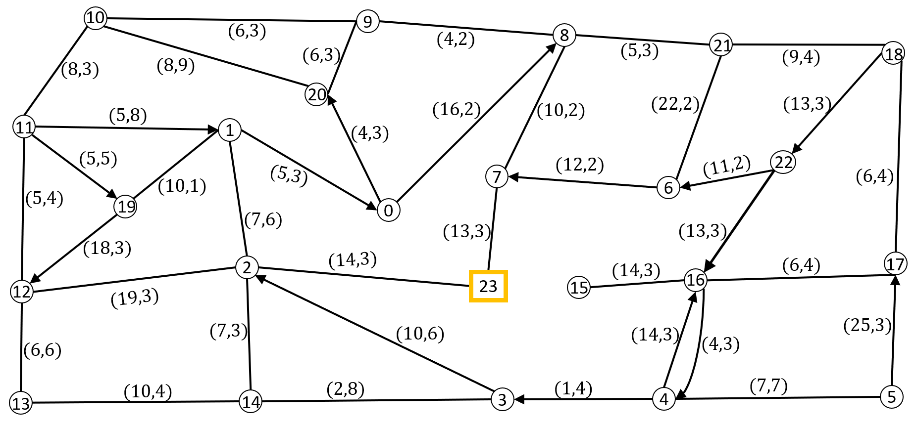
(b)

Figure 1: Test graphs for simulations. (a) Graph I and (b) Graph II. Numbers in the circles represent node index, an arrow between nodes $l$ and $k$ indicates a directed arc from $l$ to $k$ and a line without an arrow between nodes $l$ and $k$ indicates a bi-directional edge. The tuple $(a,b)$ on the arc $(l,k)$ represents $(\rho_{lk},t_{lk})$ and the Hub node $H$ is marked in square.

VI-A2 Variation of Route Set

Here, we consider the feed-in problem for the two graphs in Figure 1, that is $\mathbf{R}=\mathbf{R}_{I}$, and study the variation in $\mathcal{R}(\mathbf{R}_{I})$ as a function of the time-window, $T$ and the cost factor, $b$. Given $T$, we utilize a brute force method to enumerate all the routes in a graph. Furthermore, with $b$ and $T$, we utilize (15) and a V.o.T. of $\alpha=0.5$ to generate the best alternate transportation time and cost, $\eta_{l}$, $\zeta_{l}$ respectively, for each node $l$. Then, we use (13) to generate prices for each service tuple $(r,i,l)$.

Figure 2 shows the variation of the number of routes in $\mathbf{R}_{I}$ and $\mathcal{R}(\mathbf{R}_{I})$ as a function of $T$ for Graph I and Graph II. We see an exponentially increasing trend for the number of routes in all cases. However, as discussed in Remark IV.4, one can observe that the reduced route sets saturate eventually for large enough $T$. Moreover, the value of $T$ at which this saturation occurs increases with $b$. Finally, even prior to saturation, we see that there is a significant reduction in the route set compared to the original route set.

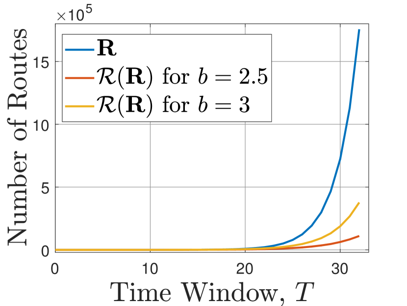
(a)

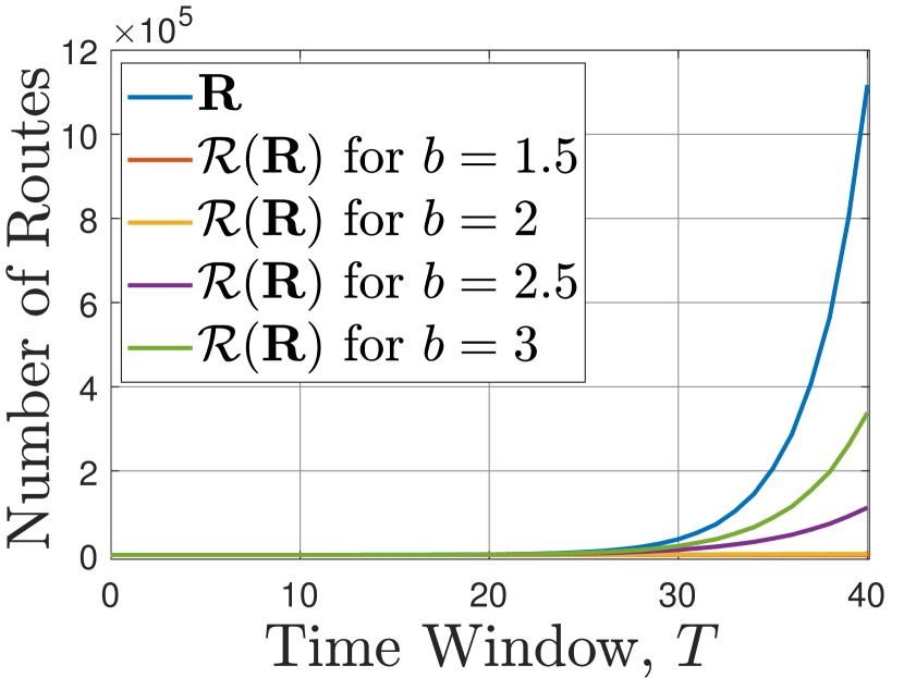
(b)

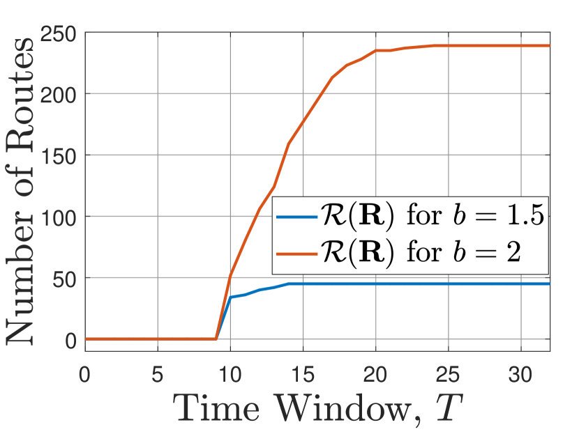
(c)

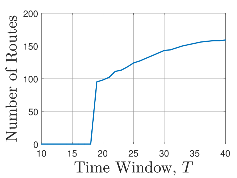
(d)

Figure 2: (a), (b): Variation of number of routes in $\mathbf{R}=\mathbf{R}_{I}$ and $\mathcal{R}(\mathbf{R}_{I})$ as a function of $T$ for Graph I and Graph II, respectively. (c), (d): Saturation observed in $\mathcal{R}(\mathbf{R}_{I})$ with $b=1.5,2$ for Graph I and with $b=1.5$ for Graph II.

Figure 3 shows the number of routes in $\mathcal{R}(\mathbf{R}_{I})$ as a function of $b$ (with a step size of 0.01) for the graphs in Figure 1.

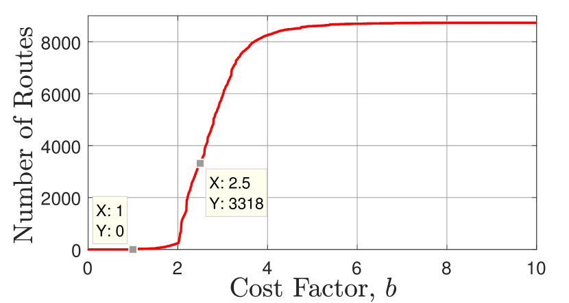
(a)

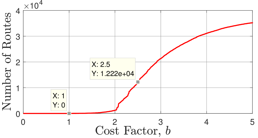
(b)

Figure 3: Variation of number of routes in $\mathcal{R}(\mathbf{R}_{I})$ versus $b$ for $\alpha=0.5$. Note that number of routes is 0 till $b=1$. (a): For Graph I and $T=20$. (b): For Graph II and $T=30$.

We note that the first route with origin as $H$ and the first multi-legged route in $\mathcal{R}(\mathbf{R}_{I})$ occur at $b=1.71$. Proposition IV.3(a), IV.3(b) and IV.3(c) give necessary lower bounds on $b$ for the existence of multi-legged routes in $\mathcal{R}(\mathbf{R}_{I})$ as $1.7027$, $1.411$ and $1.692$, respectively. As one can see, $\hat{b}_{l}^{*}$ gives a more conservative bound compared to $b_{l}^{*}$. In each case, the origin of the multi-legged route is the node $l=0$. In Figure 3, we also see that there is a significant increase in the number of routes around $b=2.1$. This can be explained by the fact that $b_{l}^{*}\in(2,2.1)$ for 5 nodes.

VI-A3 Feed-In and Comparison with Single-Depot Routing Problem for Graph II

In the rest of this subsection, we present results for Graph II. We set $b=2.5$ and $T=30$, for which $\mathcal{R}(\mathbf{R}_{I})$ has 12219 routes and 45050 optimization variables. We also note that all nodes satisfy Assumptions (A2) and (A4). We simulated the feed-in problem for a fixed demand profile with $d_{l}$, for each $l\in V$, drawn uniformly from $[0,250]_{\mathbb{Z}}$. The total demand was $\sum_{l}d_{l}=2468$. Figure 4 shows the simulation results. We utilized Proposition V.1 to generate the route set $\mathbf{R}_{I}^{-}$ which had 6265 routes and the resulting number of optimization variables was 12695. In Figure 4(a), maximum profits for given total supply (marked in red line) is from Proposition V.1. The maximum profits as a function of total supply $s$ converge to the absolute maximum profits, $J_{\max}=105033.5$ (given by Theorem V.3). We also simulated an equivalent macroscopic V.R.P., with all supply at $H$, i.e. $S_{H}=s$, $S_{l}=0$, $\forall l\neq H$. We observe in Figure 4(a) that the profits earned in this latter case are far lower, compared to that of any randomly chosen supply configurations. This is explained by two factors - insufficient time-window and cost-factor. Given $T=30$, 4 nodes do not have $r\in\mathbf{R}_{I}$ such that $o_{r}=H$ and $l\in V_{r}$. Also given $b=2.5$, only 16 of the 23 nodes satisfy Proposition (IV.3(a)), implying at-least 7 nodes do not have $r\in\mathcal{R}(\mathbf{R}_{I})$ with $o_{r}=H$ and $l\in V_{r}$. The necessary value of $b$ is $3.06$ for all nodes to satisfy Proposition IV.3(a).

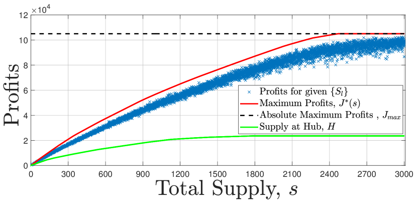
(a)

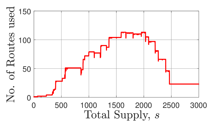
(b)

Figure 4: Simulation results for feed-in problem. (a): The red curve is the maximum profits as a function of total supply. The green curve is the maximum profits, with all supply at $H$, as a function of total supply $s$. The blue scatter points are for different supply configurations, with different supplies $s$. (b): Number of routes utilized for obtaining maximum profits in (a).

In Figure 4(b), we also see the number of routes used to generate maximum profits generally increases with $s$ though after a point the number of routes used starts to reduce. We imposed the added restriction that the supply configuration is chosen from the set (21) to compare with the equivalent feed-out problem.

VI-A4 Equivalence of Feed-Out and Feed-In Supply Optimization

We use the directed graph in Figure 1(b) and the construction in Steps (C1)-(C3) to generate a feed-out problem from the feed-in supply optimization problem. Using route set $\mathbf{\hat{R}}^{-}$, we generate the optimal profits for the same instances of total supply as before and compared it with the maximum profits for the feed-in supply optimization. The absolute error is in the range of $10^{-4}$ while the maximum relative error is $5.66\times 10^{-6}$, which is within numerical tolerance given the solver precision is $10^{-8}$ and the number of variables are 12695. This verifies the equivalence of the two problems.

VI-B Microscopic Implementation

In real life, the demands and supplies are indivisible entities, specifically integers. Thus in this section, we implement the microscopic optimization and compare it with the macroscopic optimization. Specifically, in this subsection, we assume that for each node $l$, $\tilde{d}_{l}\in{\mathbb{N}}_{0}$ and $\tilde{S}_{l}\in{\mathbb{N}}_{0}$ are the total passengers and the number of vehicles, respectively. For simplicity, we assume all the vehicles have the same capacity of $N$. In the macroscopic problem, as we assumed that a unit demand can be serviced by a unit of supply, in this subsection we assume that 1 unit of demand and supply are $N$ passengers and 1 vehicle, respectively. With this interpretation, we redefine problem (9) with integer constraints. We let $\tilde{f}_{r}^{i}(l)$ be the number of people serviced on $(r,i,l)$ and $\tilde{f}_{r}$ be the number of vehicles taking route $r$. We also assume that the operator can choose the supply configuration as in Section V. To incorporate that aspect, we assume that the operator has a total supply of $s$ at its disposal. Then the constraints discussed in (8) and (16) are modified to

$$\tilde{F}_{l}:=\sum_{(r,i)}\tilde{f}_{r}^{i}(l) \leq\tilde{d}_{l},\quad\sum_{l\in V_{r}^{i}}\tilde{f}_{r}^{i}(l)\leq N\tilde{f}_{r},\quad\sum_{r\in\mathbf{R}|o_{r}=l}\tilde{f}_{r} \leq\tilde{S}_{l},\quad\sum_{l\in V}\tilde{S}_{l}\leq s,$$ (24)

along with the integer constraints on all optimization variables.

In (10), we assumed that $\beta_{r}^{i}(l)$ is the operator income per unit demand on the service $(r,i,l)$. Therefore, the operator income per an individual passenger on the service $(r,i,l)$ is $\beta_{r}^{i}(l)/N$. Given this, the operator income from the service $(r,i,l)$ is $\tilde{f}_{r}^{i}(l)\beta_{r}^{i}(l)/N$. Further, the travelling cost incurred on route $r$ is $\tilde{f}_{r}c_{r}$. Therefore, the microscopic operator profit maximization problem is

$$\max_{\tilde{f}_{r}^{i}(l),\tilde{f}_{r},\tilde{S}_{l}}J =\sum_{(r,i,l)\in\mathbf{W}(\mathbf{R})}\tilde{f}_{r}^{i}(l)\beta_{r}^{i}(l)/N-\sum_{r\in\mathbf{R}}\tilde{f}_{r}c_{r}$$

s.t. $$\ \ \eqref{eq:discrete-constrs},\quad\tilde{f}_{r}^{i}(l),\tilde{f}_{r},\tilde{S}_{l},\tilde{F}_{l}\in{\mathbb{N}}_{0}.$$ (25)

The corresponding macroscopic problem is the same as (16). We first compare the difference in the optimal values of (25) with $\mathbf{R}=\mathbf{R}_{I}$ and $\mathbf{R}=\mathcal{R}(\mathbf{R}_{I})$ with simulations. We call these the complete micro problem and the reduced micro problem, respectively. We first show that the reduced route set is also effective for microscopic solutions. We simulated for five different vehicle capacities: 2, 4, 5, 6 and 10. Note that with integer constraints, the problem for the graphs in Figure 1 becomes rather large. Hence, for these set of simulations, we have chosen a 12 node directed graph with a time window of $T=25$ and $b=2,\ 2.5\ \&\ 3$. For $\mathbf{R}=\mathbf{R}_{I}$, the number of routes was $11694$ and the number of variables was 21127. On the other hand, the problem with $\mathbf{R}=\mathcal{R}(\mathbf{R}_{I})$ has $75$ routes and $103$ variables for $b=2$, $265$ routes and $510$ variables for $b=2.5$, and $1116$ routes and $2103$ variables for $b=3$. Gurobi required $\approx 0.35$ to $0.5$ GB of memory for the reduced micro problems (for all $b$) while it required $\approx 5$ GB of memory for the complete micro problems. The 12-node graph data is given in the supplementary material.

From Figure 5(a), we observe that the computation time ratios between the complete micro problem and the reduced micro problem for different capacities is about $25$ to $40$ times with $b=2$, $8$ to $15$ times with $b=2.5$ and $2$ to $3$ times for $b=3$. Also, from Figure 5(b) we observe that for most simulations, the optimal values returned by the complete and reduced micro problems are very similar. Only in about $4\%$ of the cases the value of the complete micro problem was higher and even then only by about $10^{-4}$ times relative to the objective value of the reduced micro problem. Since, Gurobi sometimes doesn’t converge and returns erroneous values due to lower values of MIP Gap and numerical sensitivity [36], the MIP Gap was set to 0.001 to economize on time while ensuring reliability of results.

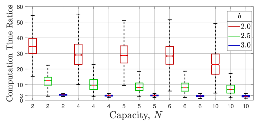
(a)

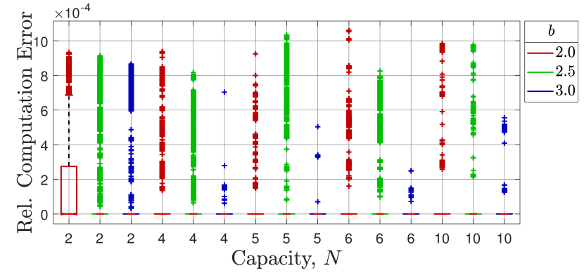
(b)

Figure 5: (a) Ratio of computation time for the complete micro problem to the computation time for the reduced micro problem for different $b$’s, and (b) Relative error of objective values between optimal solutions for the complete micro problem and the reduced micro problem on a 12 node graph for different values of $b$ and different capacities. The red, green and blue boxes represent $b=2,2.5,\text{ and }3$ respectively.

Next, we compare the macroscopic problem and the complete microscopic problem for the graphs in Figure 1. We again set time windows of $T=20$ for Graph I and $T=30$ for Graph II and $b=2.5$ and $\alpha=0.5$ for both the graphs. We chose 10 different demand configurations randomly for both the graphs in Figure 1.

Since the complete microscopic problem is very demanding in terms of both the computation time and memory requirements, we do the comparison in an indirect manner. Notice that the macroscopic problem is a relaxation of both the complete and reduced micro problems. Hence, the solutions to the macroscopic problem and the reduced micro problem provide an upper and lower bound, respectively, on the optimal objective value for the complete micro problem. Thus, by comparing these bounds, we can also indirectly compare the solutions to the macroscopic problem and the complete micro problem.

In general it is expected that with higher values of capacity $N$, the optimal values of the solutions will be far-off from the solutions obtained from (9) and the supply optimization problem proposed in Section V. Thus, for a successful implementation, the relaxation needs to find optimal solutions which are “close” to the integer optimal.

We first note the actual range of computation times of the reduced micro problem in Figure 6. We observe that the computation times generally tend to increase with $N$. This is because more branch and bound iterations are necessary to arrive at the integer optimal solution. Next, in Figure 7, we notice that the relative difference between the optimal values of reduced micro problem and the macroscopic problem is quite small, with a median of the order of $10^{-3}$. This is a reasonably small value considering the number of variables, the order of the optimal objective value and the computation power utilized for computing these solutions. Recall that the solutions to the macroscopic problem and the reduced micro problem provide upper and lower bounds, respectively, on the optimal objective value in the complete micro problem. Therefore, the relative difference between the complete micro problem and the macroscopic problem is smaller than the errors in Figure 7. Thus, the macroscopic problem is a reasonably good approximation of the reduced micro problem and thereby the complete micro problem as well. We also observed that when the demand is an integer multiple of the supply, there exists an integer solution. Furthermore, the solution was calculated in times similar to the macroscopic problem. We suspect that this behaviour is because of the fact that a unit of supply can pick-up a unit demand at one location itself and thereby no inter-node mode-sharing is required.

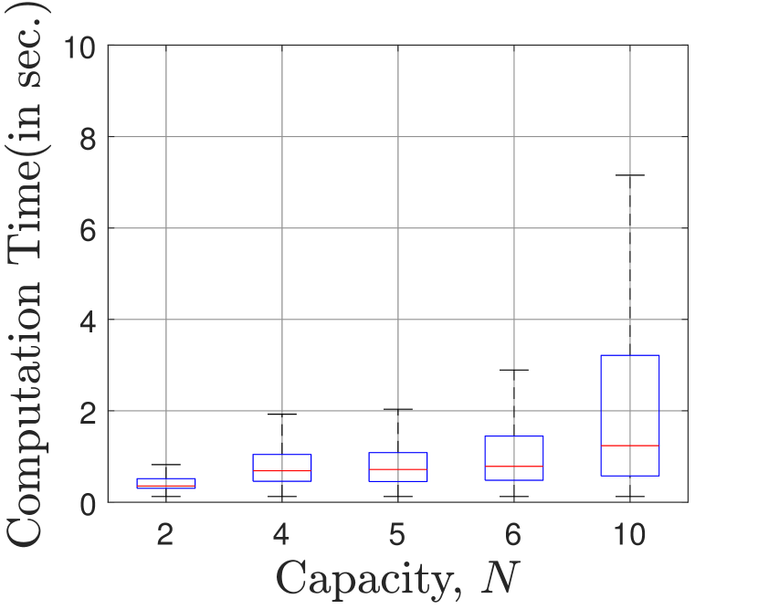
(a)

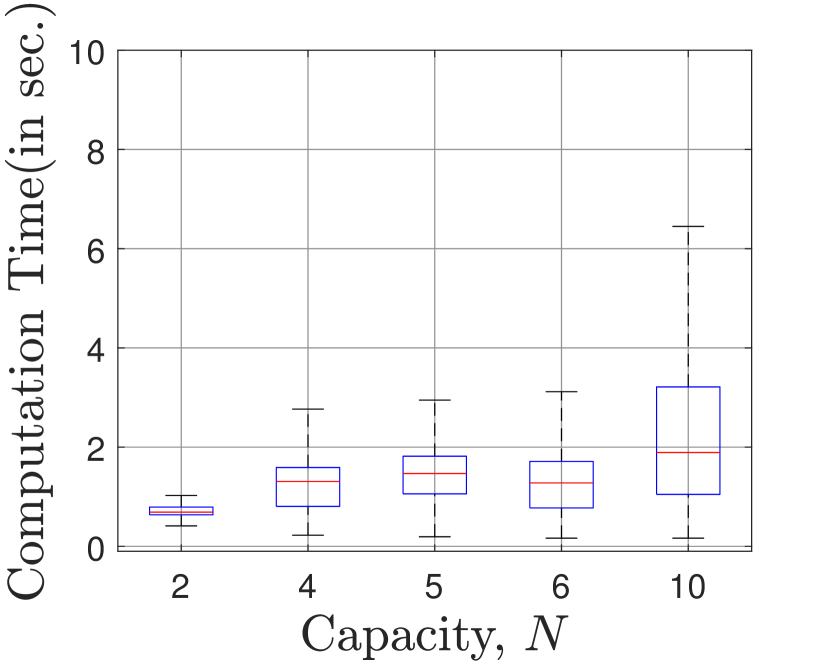
(b)

Figure 6: Computation times of optimal solutions of reduced micro problem for Graph I and II in (a) and (b), respectively.

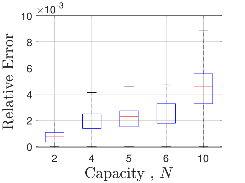
(a)

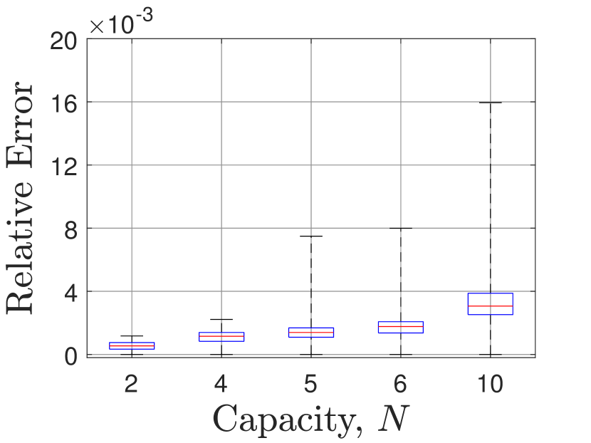
(b)

Figure 7: Relative errors between the optimal objective values of macroscopic and reduced micro problems for Graphs I and II in (a) and (b), respectively.

VI-C Pre-positioning of Relief Material for Disaster Response

As we discussed in Remark II.1 and in Section IV-B, our model can be used even in the context of routing and planning for disaster response, where the objective is not to maximize monetary profits but to maximize social welfare. In this subsection, we consider the problem of planning the routing of relief supplies post a natural disaster, such as a cyclone. The states on the eastern coast of India - West Bengal, Odisha and Andhra Pradesh - face devastating cyclones quite frequently. The scale of the disaster response is massive and often millions of people are evacuated [37, 38, 39]. Post-cyclone relief efforts are also on an equally massive scale. The most vulnerable areas generally tend to be low-lying and near the coast.

For the illustrative example here, we chose 12 coastal districts in the state of Odisha that have been severely affected in recent cyclones. The setup is as follows. The nodes in the graph are the districts and the links between the nodes are the major highways between the district headquarters. We chose the hub node as Bhubaneshwar, the capital city of the state of Odisha. We chose the link costs and travel times proportional to the distance, which we created using the Google My Maps tool. We present the map and the constructed network in Figure 8. Though the links are marked bi-directional, there are some minor asymmetries. We present the link data in the supplementary material. We look at the problem of transporting of relief material from the hub node to the remaining nodes.

We chose the demand configuration as follows. We assume that the number of affected people is 2% of the total population of each district. Furthermore, we assume that a unit demand refers to relief material for 400 people. We round off the demands to the nearest multiple of 5 and we added 10 extra units as a buffer. We assume that loading of trucks takes 2 hours. We assume that initially, all the supply of trucks is stationed at the hub node. Thus, for multi-legged routes we add a wait time of 2 hours per leg. The main goal here is to maximize the demand met while reducing transportation costs.

With this setup, we present two sets of simulation results. In the first set of simulations, for each node $l$ we chose the value of $k_{l}$ randomly in $[-5,-1]_{\mathbb{Z}}$. With these settings, we varied the total supply $s$ and the length of the time window $T$. We show the results on the demand met in Figure 9(a). As can be seen, the obvious trend is that for a fixed $T$ more demand can be met given greater supply. Similarly, for each fixed total supply $s$, longer time-windows mean more demand is met.

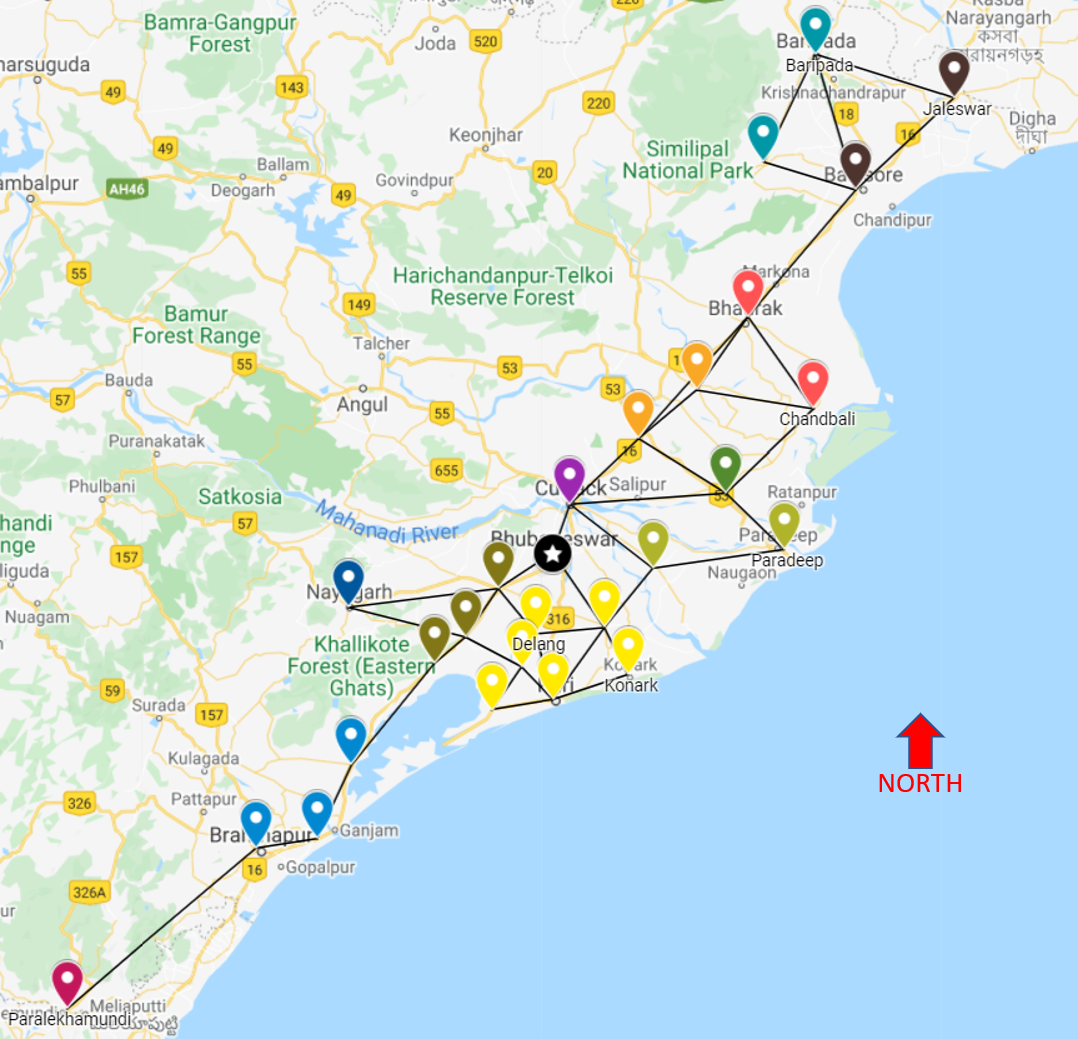
Figure 8: Map of the graph utilized for Odisha. This map was created with Google My Maps tool. Markers of same colour represent places in same district. The Hub (Bhubaneswar) is marked with a black star.

In the second set of simulations, we fix the window time $T=12$ and fix the values of $k_{l}$ to the same value for all nodes $l$. Figure 9(b) shows the simulation results for different values of supply $s$ and different values of $k_{l}$. For each fixed supply, as we increase the magnitude of $k_{l}$ more demand is met. Thus, in general, $k_{l}$ can be made proportional to the severity of the cyclone in a given region/node $l$ to divert the supplies accordingly.

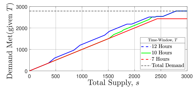
(a)

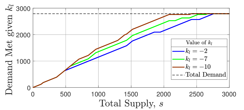
(b)

Figure 9: Simulation results for the Odisha supply prepositioning model. (a): Demand met given different window times $T$. (b): Demand met given window time, $T=12$ hours and different values of $k_{l}$.

VII Conclusions

In this paper, we proposed a problem of one-shot coordination of first mode or last mode transportation service, wherein an operator seeks to maximize its profits or social welfare with routing and allocation, for transporting a known demand to or from a common destination on a network in a given fixed time window. We posed the problem in a macroscopic setting where we considered all supplies and demands as volumes. Using K.K.T. analysis we were able to design an offline (supply and demand independent) method that reduces the complexity of the online (after supply and demand are revealed) optimization. Then, we considered the feed-in supply optimization problem, analyzed its properties and computed the absolute maximum profits that the operator can earn over all possible supply configurations for a given demand configuration. We showed an equivalence between the feed-in supply optimization problem and the one-shot feed-out problem, wherein the operator needs to drop-off people to their destinations from a common origin within a fixed time window. This allows us to directly apply the results and algorithms developed for the feed-in problem. We presented a pricing model and derived necessary conditions for the feeder service to be viable. Finally, we presented several simulation results to illustrate our analytical results. Through simulations, we also demonstrated that the route reduction algorithm that we proposed for the macroscopic formulation is still useful for efficiently computing the solutions to the microscopic formulation, in which the decision variables are all integers. We also explored a realistic scenario of disaster response.

Future work includes improvements in the route reduction algorithm, perhaps making it also dependent on the demand and supply configurations, a more rigorous study of the macroscopic formulation and the route reduction algorithm as a computationally efficient solution method for the microscopic formulation; extension to a multiple time window problem, load balancing of the supply in accordance with the anticipated demand using the insights from the feed-in supply optimization problem, extension to the scenario with uncertainty about supply and demand and finally an integrated coordination of multiple modes of transportation.

VIII Acknowledgements

We wish to thank Dr. Tarun Rambha of Department of Civil Engineering at the Indian Institute of Science (IISc), Bengaluru for his valuable comments and suggestions.

-A Proofs of Results on General One-Shot Feeding Problem

-A1 Proof of Proposition III.1

We first introduce the Lagrangian $\mathcal{L}$ for the problem (9),

$$\mathcal{L}=J+\sum_{l\in V}\mu_{l}(\sum_{r,i}f_{r}^{i}(l)-d_{l})+\sum_{r,i}\lambda_{r}^{i}(\sum_{l\in V_{r}^{i}}f_{r}^{i}(l)-f_{r})+\sum_{l\in V}\gamma_{l}(\sum_{r|o_{r}=l}f_{r}-S_{l})-\sum_{r}\delta_{r}f_{r}-\sum_{r,l,i}\delta_{r}^{i}(l)f_{r}^{i}(l),$$ (26)

where $\mu_{l},\lambda_{r}^{i},\gamma_{l},\delta_{r},\delta_{r}^{i}(l)\leq 0$ are the KKT multipliers. The stationarity and complementary slackness conditions are

$$\frac{\partial\mathcal{L}}{\partial f_{r}^{i}(l)}=\beta_{r}^{i}(l)+\mu_{l}+\lambda_{r}^{i}-\delta_{r}^{i}(l)=0$$ (27a)

$$\frac{\partial\mathcal{L}}{\partial f_{r}}=-c_{r}-\sum_{i}\lambda_{r}^{i}+\gamma_{o_{r}}-\delta_{r}=0$$ (27b)

$$\mu_{l}(\sum_{r,i}f_{r}^{i}(l)-d_{l})=0,\quad\lambda_{r}^{i}(\sum_{l\in V_{r}^{i}}f_{r}^{i}(l)-f_{r})=0$$ (27c)

$$\gamma_{l}(\sum_{r|o_{r}=l}f_{r}-S_{l})=0,\quad\delta_{r}^{i}(l)f_{r}^{i}(l)=0,\quad\delta_{r}f_{r}=0.$$ (27d)

(a): In an optimal solution, if $f_{r}^{*}>0$ then $\delta_{r}^{*}=0$. Further as $\gamma_{o_{r}}^{*}\leq 0$ and $c_{r}>0$, we can use (27b) to obtain

$$\sum_{i=1}^{\theta_{r}}{\lambda_{r}^{i}}^{*}=-c_{r}+\gamma_{o_{r}}^{*}<0.$$ (28)

Thus, we see from (27c) that $\displaystyle\sum_{l\in V_{r}^{i}}f_{r}^{i}(l)^{*}=f_{r}^{*}$ for at least one leg $i$ in the route $r$. Hence we must have $f_{r}^{i}(l)^{*}>0$ for some $i\in[1,\theta_{r}]_{\mathbb{Z}}$ and $l\in V_{r}^{i}$. Now, if $f_{r}^{i}(l)^{*}>0$ then $\delta_{r}^{i}(l)=0$. Hence condition (27a) implies

$$\beta_{r}^{i}(l)=-{\lambda_{r}^{i}}^{*}-\mu_{l}^{*}\geq-{\lambda_{r}^{i}}^{*}\geq 0,\text{ if }f_{r}^{i}(l)^{*}>0.$$ (29)

(b): We prove this by contradiction. Let us assume that there exists some optimal solution such that (11) does not hold for a circular leg $i$ of some $r\in\mathbf{R}$. Then, $\delta:=f_{r}^{*}-\sum f_{r}^{i}(l)^{*}>0$ units of flow costs $\delta c_{r}^{i}$ while earning no revenue.

Now consider a route $\bar{r}$ that follows the same sequence of nodes as $r$ but without the $i^{\text{th}}$ leg of $r$. We can construct another feasible solution with $f_{r}=f_{r}^{*}-\delta$ and $f_{\bar{r}}=f_{\bar{r}}^{*}+\delta$ with all the other flows and allocations remaining the same. Now leg $i$ of route $r$ in this solution satisfies (11). Such a solution is feasible and does not lose $\delta c_{r}^{i}$ while earning same revenue. Thus, this solution earns more profit than the optimal solution, which is a contradiction.

(c): Notice that $f_{r}^{i}(l)^{*}\beta_{r}^{i}(l)\geq-f_{r}^{i}(l)^{*}{\lambda_{r}^{i}}^{*}$ for each $(r,i,l)$, since if $f_{r}^{i}(l)=0$ then the inequality holds trivially and if $f_{r}^{i}(l)>0$ then the condition (29) holds, which implies

$$\sum_{i=1}^{\theta_{r}}\sum_{l\in V_{r}^{i}}f_{r}^{i}(l)^{*}\beta_{r}^{i}(l) \geq-\sum_{i=1}^{\theta_{r}}\sum_{l\in V_{r}^{i}}f_{r}^{i}(l)^{*}{\lambda_{r}^{i}}^{*}.$$

Now, using part (b), we obtain

$$\sum_{i=1}^{\theta_{r}}\sum_{l\in V_{r}^{i}}f_{r}^{i}(l)^{*}\beta_{r}^{i}(l)\geq-\sum_{l\in V_{r}^{1}}f_{r}^{1}(l)^{*}{\lambda_{r}^{1}}^{*}-f_{r}^{*}\sum_{i=2}^{\theta_{r}}{\lambda_{r}^{i}}^{*}.$$

From the K.K.T. conditions, we either have ${\lambda_{r}^{1}}^{*}=0$ or $\sum_{l\in V_{r}^{1}}f_{r}^{1}(l)^{*}=f_{r}^{*}$. In either case, we have

$$\sum_{i=1}^{\theta_{r}}\sum_{l\in V_{r}^{i}}f_{r}^{i}(l)^{*}\beta_{r}^{i}(l)\geq-f_{r}^{*}\sum_{i=1}^{\theta_{r}}{\lambda_{r}^{i}}^{*}\geq f_{r}^{*}c_{r},$$

where the second inequality follows from (28).

(d): Now due to Part (c), if $f_{r}^{*}>0$ then $\forall$ $i>1$, $\exists$ $l\in V_{r}^{i}$ such that $f_{r}^{i}(l)^{*}>0$. In any feasible solution, for $i>1$, if $\beta_{r}^{i}(l)<c_{r}^{i}$ and $f_{r}^{i}(l)>0$ then we can construct another feasible solution in which $f_{r}^{i}(l)=0$ keeping all other node allocation variables unchanged. The value of the objective is strictly more with such a new solution. Thus, $\beta_{r}^{i}(l)\geq c_{r}^{i}$ if $f_{r}^{i}(l)^{*}>0$ for $i>1$ in an optimal solution of Problem (9). If $i=1$ and leg $1$ of route $r$ is circular then according to a similar argument as above, we must again have at least one $l\in V_{r}^{1}$ such that $f_{r}^{1}(l)^{*}>0$ and for each such $l$, $\beta_{r}^{1}(l)\geq c_{r}^{1}$.

(e): In part (c), by setting $\theta_{r}=1$, we get

$$\sum_{l\in V_{r}^{1}}f_{r}^{1}(l)^{*}\beta_{r}^{1}(l)\geq f_{r}^{*}c_{r}.$$

Similarly, setting $\theta_{r}=1$ in (28) gives us $\lambda_{r}^{1}\leq-c_{r}<0$, which along with (27c) means that in any optimal solution, constraint (8b) is a strict equality for single legged routes. Therefore, we have $\sum_{l\in V_{r}^{1}}(\beta_{r}^{1}(l)-c_{r})f_{r}^{1}(l)^{*}\geq 0$. Now, part (e) follows in the same way as part (d). ∎

-B Proofs of Results on Best Transportation Parameters

-B1 Proof of Lemma IV.2

Consider an arbitrary node $l\in V$ and a service tuple $(r,i,l)$ such that $l\in V_{r}^{i}$. Then, from (13) and (10) notice that

$$\beta_{r}^{i}(l)-c_{r}^{i} =g_{l}(b)-\alpha t_{r}^{i}(l)-c_{r}^{i}-k_{l}\leq g_{l}(b)-g_{l}(1)-k_{l}$$

where $g_{l}(b)$ is as defined in (15). The inequality follows from the fact that a leg is also single legged route and therefore $g_{l}(1)$ lower bounds $\alpha t_{r}^{i}(l)-c_{r}^{i}$. Thus it is easy to see that $\beta_{r}^{i}(l)-c_{r}^{i}\geq 0$ and hence $\mathcal{R}(\mathbf{R})\neq\emptyset$ only if $g_{l}(b)\geq g_{l}(1)+k_{l}$. Now, we show that if $\exists l\in V$ such that $g_{l}(b)\geq g_{l}(1)+k_{l}$, then $\mathcal{R}(\mathbf{R})\neq\emptyset$. We show that $r(l,1)^{*}\in\mathcal{R}(\mathbf{R})$ for this case. Thus, considering $q=r(l,1)^{*}$, as per Table I, we have

$$\beta_{q}^{1}(l)-c_{q}^{1}=g_{l}(b)-\alpha t_{q}^{1}(l)-k_{l}-c_{q}^{1}=g_{l}(b)-(\alpha t_{q}+c_{q}+k_{l})=g_{l}(b)-(g_{l}(1)+k_{l})\geq 0.$$

Thus, $q\in\mathbf{R}_{1}$ which implies $\mathcal{R}(\mathbf{R})\neq\emptyset$, if $g_{l}(b)\geq g_{l}(1)+k_{l}$.

Now, we know from Remark IV.1 that $g_{l}(b)$ is an increasing function of $b$. Thus, for $k_{l}\geq 0$, $b\geq 1$ is necessary to ensure $\mathcal{R}(\mathbf{R})\neq\emptyset$. Again, for $k_{l}<0$ for some $l\neq H$, and $b=1$, $g_{l}(b)-g_{l}(1)-k_{l}\geq 0$, following the discussion above. ∎

-B2 Proof of Proposition IV.3

Consider a route $r\in\mathcal{R}(\mathbf{R})$ with two distinct legs with feasible services. Note that such a route, has atleast one leg, $i$ with $o_{r}^{i}=D_{r}^{i}=H$. Also, route $r\in\mathbf{R}_{2}$ (see (12c)) as $\theta_{r}\geq 2$. Now, let $\bar{r}$ be the route that is same as leg $i$ of route $r$. Thus, $o_{\bar{r}}=D_{\bar{r}}=H$, $\theta_{\bar{r}}=1$ and $w_{\bar{r}}^{1}\geq 0$, which implies $\bar{r}\in\mathcal{R}(\mathbf{R})$ as $\bar{r}\in\mathbf{R}_{1}$ (see (12b)). Hence, from (13) and (10), $\displaystyle w_{\bar{r}}^{1}=\max_{l\in V_{\bar{r}}^{1}}\{\beta_{\bar{r}}^{1}(l)-c_{\bar{r}}\}\geq 0$ implies

$$g_{l}(b)\geq\alpha t_{\bar{r}}^{1}(l)+c_{\bar{r}}+k_{l},\text{ for some }l\in V_{\bar{r}},\ l\neq H,$$ (30)

where we have used the fact that $g_{H}(b)=0$ for all $b\geq 0$ and $k_{H}>0$, which imply that $l\neq H$. Now, note that for

$$\alpha t_{\bar{r}}^{1}(l)+c_{\bar{r}} =\alpha t_{\bar{r}}^{1}(l)+c_{\bar{r}}(H,l)+c_{\bar{r}}(l,H)$$

$$\geq\begin{cases}g_{l}(1)+c^{*}(H,l),&\text{ if }\mathbf{R}=\mathbf{R}_{I}\\ g_{l}(1)+c^{*}(l,H),&\text{ if }\mathbf{R}=\mathbf{R}_{O}\end{cases}$$

$$=g_{l}(1)+c^{*}(D,O)$$

where we have split the route cost $c_{\bar{r}}$ into $c_{\bar{r}}(H,l)$, the cost to go from $H$ to $l$ on route $\bar{r}$, and $c_{\bar{r}}(l,H)$, the cost to go back from $l$ to $H$. Therefore, from (30), $g_{l}(b)\geq g_{l}(1)+c^{*}(D,O)+k_{l}$, thus proving claim (a).

Now using (15), we get $g_{l}(b)=\alpha t_{r(l,b)^{*}}+bc_{r(l,b)^{*}}$ and $g_{l}(1)=\alpha t_{r(l,1)^{*}}+c_{r(l,1)^{*}}$. Therefore, claim (b) is true.

Next, from Lemma IV.2, we know that if $k_{l}>0$ for all $l\in V$ then $\mathcal{R}(\mathbf{R})$ is non-empty only if $b>1$. Then, notice from (14) and (15) that $c_{r(l,0)^{*}}\geq c_{r(l,1)^{*}}\geq c_{r(l,b)^{*}}$ and $t_{r(l,b)^{*}}\leq t_{r(l,\infty)^{*}}$. Using these facts we obtain claim (c). Finally, as $c_{r(l,b)^{*}}$ is a non-increasing function of $b$ we conclude that $b_{l}^{*}\geq\hat{b}_{l}^{*}$. ∎

-C Proofs of Results on Feed-in Supply Optimization

-C1 Proof of Proposition V.1

Part (a) is true because Theorem III.2 applies for every possible supply configuration. We prove the remaining parts by contradiction.

(b): Let us assume there exists an optimal solution, which we denote using a superscript $*$, in which $f_{r}^{*}>0$ for a route $r\in\mathcal{R}(\mathbf{R}_{I})$ such that $f_{r}^{1}(o_{r})^{*}<f_{r}^{*}$. Then, there are the following two cases. (i) $f_{r}^{1}(o_{r})^{*}>0$ and $f_{r}^{i}(l)^{*}=0$ for all other legs and nodes $(i,l)$ on route $r$; and (ii) there is a pair $(i_{1},l_{1})\in[1,\theta_{r}]_{\mathbb{Z}}\times V_{r}$ with $(i_{1},l_{1})\neq(1,o_{r})$ and $f_{r}^{i_{1}}(l_{1})^{*}>0$. Note that Proposition III.1(b) implies that scenario (i) may occur only if the route is simple ($\theta_{r}=1$).

(i) In this case, clearly the original solution cannot be optimal because $f_{r}^{*}-f_{r}^{1}(o_{r})^{*}$ volume of vehicles simply traverse the route without serving any demand, thus incurring a non-zero cost while earning nothing.

(ii) Without loss of generality let $(i,l_{1})$ be the leg, node pair other than $(1,o_{r})$ that first appears in the sequence given by the route $r$ such that $f_{r}^{i}(l_{1})^{*}>0$. Then consider the route $\bar{r}$, which is the sub-route of $r$ formed by excluding all nodes in $r$ that occur prior to $(i,l_{1})$ so that $o_{\bar{r}}=l_{1}$. Thus, for each leg and node pair $(j,m)$ of the route $\bar{r}$ there is a unique leg and node pair $(k,l)$ of route $r$ such that $(j-i+1,m)=(k,l)$ and moreover they appear in the same order. Now consider a solution $f_{r}=f_{r}^{1}(o_{r})=f_{r}^{1}(o_{r})^{*}$ and $f_{\bar{r}}=f_{\bar{r}}^{*}+(f_{r}^{*}-f_{r}^{1}(o_{r})^{*})$ and such that $f_{\bar{r}}^{j}(m)+f_{r}^{k}(l)=f_{\bar{r}}^{j}(m)^{*}+f_{r}^{k}(l)^{*}$ for every $m\in V_{\bar{r}}^{i}$ and for each leg $j$ of route $\bar{r}$. This solution is feasible and earns higher profits than the original solution as the flow $(f_{r}^{*}-f_{r}^{1}(o_{r})^{*})$ does not have to traverse the sequence of nodes from $(1,o_{r})$ to $(i,l_{1})$ and the node allocations are unchanged. This again contradicts the assumption that the original solution is optimal. Thus, for each $r\in\mathcal{R}(\mathbf{R}_{I})$, $f_{r}^{1}(o_{r})^{*}=f_{r}^{*}$. As a consequence of this fact and Proposition III.1(b), we also have (17). Also, $d_{H}=0$ implies $f_{r}^{*}=0$, $\forall r$ s.t. $o_{r}=H$.

(c): Assume an optimal solution with $f_{r}^{*}>0$, for a $r\in\mathcal{R}(\mathbf{R}_{I})$ with $\beta_{r}^{1}(o_{r})<c_{r}^{1}$. Using (b), we know $f_{r}^{1}(o_{r})^{*}=f_{r}^{*}>0$. However, one could set $f_{r}^{1}(o_{r})^{*}=0$ and move the supply on $o_{r}$ as in part (b). Then, the so constructed solution would again earn higher profits, which contradicts the assumption that the original solution is optimal. Consequently, with Proposition III.1(d), $\exists\ l\in V_{r}^{i},\ s.t.\ f_{r}^{i}(l)^{*}>0,\ \beta_{r}^{i}(l)\geq c_{r}^{i},\forall i\in[1,\theta_{r}]_{\mathbb{Z}}$ .

(d): Suppose that a node $l$ violates the property in  (A4) and yet $f_{r}^{i}(l)^{*}>0$ for some route $r$ and a leg $i$. Then by part (c) we must have $\beta_{r}^{i}(l)-c_{r}^{i}\geq 0$. Now, given the service tuple $(r,i,l)$, consider a simple route $q$, which is the sub-route of route $r$ from the last visit to node $l$ in leg $i$ to $H$ in that leg. As a result, $o_{q}=l$ and $q\in\mathbf{R}_{I}$. Now, notice that

$$\beta_{q}^{1}(l)-c_{q}^{1}\geq\beta_{r}^{i}(l)-c_{r}^{i}\geq 0,$$

since $q$ is a sub-route of the leg $i$ of route $r$. This contradicts the assumption that $l$ violates the property in (A4).

(e): One can construct another route $q$ from $r$ by avoiding the cycle. Again, moving the supply to this route (in a manner similar to the previous parts) earns more profits.

(f): In the scenario $s\leq\sum_{l}d_{l}$, the key observation is that the full demand cannot be served by simple routes. Thus, if $\displaystyle\sum_{r|o_{r}=l}f_{r}^{*}<S_{l}$ for some node $l\in V$ then there is some unused supply. Such redundant supply could potentially be used to serve more demand either at node $l$ or moved to a different node $\bar{l}$ to meet the demand there with simple routes. Assumption (A4) implies that there exist simple routes to which if the redundant supply is reallocated then the profits are higher. This contradicts the assumption that the original solution is optimal. Thus, in every optimal solution, we have

$$S_{l}=\displaystyle\sum_{r|o_{r}=l}f_{r}^{*}\leq F_{l}^{*}\leq d_{l},\quad\forall l\in V,$$

where the second inequality is just one of the constraints in the optimization problem. ∎

-C2 Proof of Lemma V.2

By the definition of $\mathcal{S}(l)$ in (20), $\beta_{r}^{1}(l)-c_{r}>\beta_{q}^{1}(l)-c_{q}$, $\forall\ r\in\mathcal{S}(l)$ and $\forall q\in(\sigma(l)\setminus\mathcal{S}(l))$. Every other route $\bar{r}$ either originates from a different location or has multiple legs and in each case the leg/route cost is higher and the operator incomes are lower. Therefore, $\exists q\in(\sigma(l)\setminus\mathcal{S}(l))$ for which $\beta_{q}^{1}(l)-c_{q}>\beta_{\bar{r}}^{i}(l)-c_{\bar{r}}^{i}$. Hence, $\beta_{r}^{1}(l)-c_{r}>\beta_{\bar{r}}^{i}(l)-c_{\bar{r}}^{i}$ for all $r\in\mathcal{S}(l)$ and $\bar{r}\notin\mathcal{S}(l)$. Further, for $\forall r\in\mathcal{S}(l)$ and $\forall q\in(\sigma(l)\setminus\mathcal{S}(l))$, the perceived costs satisfy

$$(\alpha t_{r}+c_{r})-(\alpha t_{q}+c_{q})=(\alpha t_{r}+c_{r}-g_{l}+1)-(\alpha t_{q}+c_{q}-g_{l}+1)=-(\beta_{r}^{1}(l)-c_{r})+(\beta_{q}^{1}(l)-c_{q})<0,$$ (31)

where we have used (13) and (10) and the fact that $o_{z}=l$ for all $z\in\sigma(l)$, which implies that the route traversal time $t_{z}=t_{z}^{1}(l)$. This proves the result. ∎

-C3 Proof of Lemma V.5

As for both the problems, the time window, best travel cost and the best travel time are same, it therefore suffices to show that $t_{\bar{r}}^{\theta_{r}-i+1}(l)=\hat{t}_{r}^{i}(l)$. Note that the $i^{\text{th}}$ leg of $r$ is same as the $(\theta_{r}-i+1)^{\text{th}}$ leg of $\bar{r}$ in reverse. Also, $T-t_{\bar{r}}^{\theta_{r}-i+1}(l)$ is the last possible pick-up time along $(\bar{r},\theta_{r}-i+1,l)$, based on the observations of (13) which implies that $T-t_{\bar{r}}^{\theta_{r}-i+1}(l)$ is the first possible drop-off time for the reverse route $r$ along the service tuple $(r,i,l)$. ∎

References

- [1] S. Goswami and P. Tallapragada, “One-shot coordination of feeder vehicles for multi-modal transportation,” in European Control Conference, Naples, Italy, 2019, pp. 1714–1719.
- [2] V. Campos, R. Bandeira, and A. Bandeira, “A method for evacuation route planning in disaster situations,” Procedia-Social and Behavioral Sciences, vol. 54, pp. 503–512, 2012.
- [3] R. Lave and R. R. Mathias, “State of the art of paratransit,” Transportation in the New Millennium, vol. 478, pp. 1–7, 2000.
- [4] M. SteadieSeifi, N. Dellaert, W. Nuijten, T. V. Woensel, and R. Raoufi, “Multimodal freight transportation planning: A literature review,” European journal of operational research, vol. 233, no. 1, pp. 1–15, 2014.
- [5] C. Barnhart, N. Krishnan, D. Kim, and K. Ware, “Network design for express shipment delivery,” Computational Optimization and Applications, vol. 21, no. 3, pp. 239–262, 2002.
- [6] H. Min, “The multiple vehicle routing problem with simultaneous delivery and pick-up points,” Transportation Research Part A: General, vol. 23, no. 5, pp. 377–386, 1989.
- [7] P. Toth and D. Vigo, The vehicle routing problem. SIAM, 2002.
- [8] F. Ferrucci, Pro-active Dynamic Vehicle Routing: Real-time Control and Request-forecasting Approaches to Improve Customer Service. Springer Science & Business Media, 2013.
- [9] M. W. Ulmer, Approximate Dynamic Programming for Dynamic Vehicle Routing, 1st ed. Springer International Publishing, 2017.
- [10] T. Vidal, G. Laporte, and P. Matl, “A concise guide to existing and emerging vehicle routing problem variants,” European Journal of Operational Research, 2019.
- [11] N. Agatz, A. Erera, M. Savelsbergh, and X. Wang, “Optimization for dynamic ride-sharing: A review,” European Journal of Operational Research, vol. 223, no. 2, pp. 295–303, 2012.
- [12] J. Alonso-Mora, S. Samaranayake, A. Wallar, E. Frazzoli, and D. Rus, “On-demand high-capacity ride-sharing via dynamic trip-vehicle assignment,” Proceedings of the National Academy of Sciences, vol. 114, no. 3, pp. 462–467, 2017.
- [13] F. Vincent, S. Purwanti, A. Redi, C. Lu, S. Suprayogi, and P. Jewpanya, “Simulated annealing heuristic for the general share-a-ride problem,” Engineering Optimization, vol. 50, no. 7, pp. 1178–1197, 2018.
- [14] C. Tao and C. Chen, “Heuristic algorithms for the dynamic taxipooling problem based on intelligent transportation system technologies,” in 4th International conference on fuzzy systems and knowledge. IEEE, 2007, pp. 590–595.
- [15] J. Cordeau and G. Laporte, “The dial-a-ride problem: models and algorithms,” Annals of operations research, vol. 153, no. 1, pp. 29–46, 2007.
- [16] S. Ho, W. Szeto, Y. Kuo, J. Leung, M. Petering, and T. Tou, “A survey of dial-a-ride problems: Literature review and recent developments,” Transportation Research Part B: Methodological, 2018.
- [17] B. Li, D. Krushinsky, H. Reijers, and T. V. Woensel, “The share-a-ride problem with stochastic travel times and stochastic delivery locations,” Transportation Research Part C: Emerging Technologies, vol. 67, pp. 95–108, 2016.
- [18] K. Seow, N. Dang, and D. Lee, “A collaborative multiagent taxi-dispatch system,” IEEE Transactions on Automation Science and Engineering, vol. 7, no. 3, pp. 607–616, 2010.
- [19] F. Miao, S. Han, S. Lin, J. Stankovic, D. Zhang, S. Munir, H. Huang, T. He, and G. Pappas, “Taxi dispatch with real-time sensing data in metropolitan areas: A receding horizon control approach,” IEEE Transactions on Automation Sciences and Engineering, vol. 13, no. 2, pp. 463–478, 2016.
- [20] F. Rossi, R. Zhang, Y. Hindy, and M. Pavone, “Routing autonomous vehicles in congested transportation networks: structural properties and coordination algorithms,” Autonomous Robots, pp. 1–16, 2017.
- [21] M. Salazar, F. Rossi, M. Schiffer, C. Onder, and M. Pavone, “On the interaction between autonomous mobility-on-demand and public transportation systems,” arXiv preprint arXiv:1804.11278, 2018.
- [22] M. Pavone, S. Smith, E. Frazzoli, and D. Rus, “Robotic load balancing for mobility-on-demand systems,” International Journal of Robotics Research, vol. 31, no. 7, pp. 839–854, 2012.
- [23] R. Zhang and M. Pavone, “Control of robotic mobility-on-demand systems: a queueing-theoretical perspective,” The International Journal of Robotics Research, vol. 35, no. 1-3, pp. 186–203, 2016.
- [24] A. Vakayil, W. Gruel, and S. Samaranayake, “Integrating shared-vehicle mobility-on-demand systems with public transit,” in 96th Annual Meeting of Transportation Research Board. T.R.B., 2017.
- [25] S. Shaheen and N. Chan, “Mobility and the sharing economy: Potential to facilitate the first-and last-mile public transit connections,” Built Environment, vol. 42, no. 4, pp. 573–588, 2016.
- [26] A. M. Caunhye, X. Nie, and S. Pokharel, “Optimization models in emergency logistics: A literature review,” Socio-economic planning sciences, vol. 46, no. 1, pp. 4–13, 2012.
- [27] G. Galindo and R. Batta, “Review of recent developments in or/ms research in disaster operations management,” European Journal of Operational Research, vol. 230, no. 2, pp. 201–211, 2013.
- [28] M. S. Habib, Y. H. Lee, and M. S. Memon, “Mathematical models in humanitarian supply chain management: A systematic literature review,” Mathematical Problems in Engineering, vol. 2016, 2016.
- [29] M. Sabbaghtorkan, R. Batta, and Q. He, “Prepositioning of assets and supplies in disaster operations management: Review and research gap identification,” European Journal of Operational Research, vol. 284, no. 1, pp. 1–19, 2020.
- [30] M. Ahmadi, A. Seifi, and B. Tootooni, “A humanitarian logistics model for disaster relief operation considering network failure and standard relief time: A case study on san francisco district,” Transportation Research Part E: Logistics and Transportation Review, vol. 75, pp. 145–163, 2015.
- [31] M. Huang, K. Smilowitz, and B. Balcik, “Models for relief routing: Equity, efficiency and efficacy,” Transportation research part E: logistics and transportation review, vol. 48, no. 1, pp. 2–18, 2012.
- [32] J. M. Ferrer, F. J. Martín-Campo, M. T. Ortuño, A. J. Pedraza-Martínez, G. Tirado, and B. Vitoriano, “Multi-criteria optimization for last mile distribution of disaster relief aid: Test cases and applications,” European Journal of Operational Research, vol. 269, no. 2, pp. 501–515, 2018.
- [33] A. M. Campbell, D. Vandenbussche, and W. Hermann, “Routing for relief efforts,” Transportation Science, vol. 42, no. 2, pp. 127–145, 2008.
- [34] R. Liu and Z. Jiang, “A hybrid large-neighborhood search algorithm for the cumulative capacitated vehicle routing problem with time-window constraints,” Applied Soft Computing, vol. 80, pp. 18–30, 2019.
- [35] S. Diamond and S. Boyd, “CVXPY: A Python-embedded modeling language for convex optimization,” Journal of Machine Learning Research, vol. 17, no. 83, pp. 1–5, 2016.
- [36] L. Gurobi Optimization, “Gurobi optimizer reference manual,” 2021. [Online]. Available: http://www.gurobi.com
- [37] B. S. Correspondent, “India cyclone fani evacuation efforts hailed a success,” BBC, 4 May, 2019. [Online]. Available: https://www.bbc.com/news/world-asia-48160096
- [38] L. Lear, “Amphan: India and bangladesh evacuate millions ahead of super cyclone,” BBC, 19 May, 2020. [Online]. Available: https://www.bbc.com/news/world-asia-india-52718826
- [39] J. Slater and N. Masih, “Cyclone amphan batters india and bangladesh, leaving at least 14 dead,” The Washington Post, 20 May, 2020. [Online]. Available: https://wapo.st/2TPKkC3