On Kostant’s weight $q$-multiplicity formula for $\mathfrak{sl}_{4}(\mathbb{C})$

Abstract.

The $q$-analog of Kostant’s weight multiplicity formula is an alternating sum over a finite group, known as the Weyl group, whose terms involve the $q$-analog of Kostant’s partition function. This formula, when evaluated at $q=1$, gives the multiplicity of a weight in a highest weight representation of a simple Lie algebra. In this paper, we consider the Lie algebra $\mathfrak{sl}_{4}(\mathbb{C})$ and give closed formulas for the $q$-analog of Kostant’s weight multiplicity. This formula depends on the following two sets of results. First, we present closed formulas for the $q$-analog of Kostant’s partition function by counting restricted colored integer partitions. These formulas, when evaluated at $q=1$, recover results of De Loera and Sturmfels. Second, we describe and enumerate the Weyl alternation sets, which consist of the elements of the Weyl group that contribute nontrivially to Kostant’s weight multiplicity formula. From this, we introduce Weyl alternation diagrams on the root lattice of $\mathfrak{sl}_{4}(\mathbb{C})$, which are associated to the Weyl alternation sets. This work answers a question posed in 2019 by Harris, Loving, Ramirez, Rennie, Rojas Kirby, Torres Davila, and Ulysse.

1. Introduction

Let $\mathfrak{g}$ be a simple Lie algebra of rank $r$ and $\mathfrak{h}$ be a Cartan subalgebra of $\mathfrak{g}$. We let $\Phi$ denote the set of roots corresponding to $(\mathfrak{g},\mathfrak{h})$, $\Phi^{+}\subset\Phi$ denote a set of positive roots, and $\Delta\subset\Phi^{+}$ denote a set of simple roots. Throughout, we let $\alpha_{1},\alpha_{2},\ldots,\alpha_{r}$ denote the simple roots, $\varpi_{1},\varpi_{2},\ldots,\varpi_{r}$ denote the fundamental weights, $P(\mathfrak{g}):=\{c_{1}\varpi_{1}+\cdots+c_{r}\varpi_{r}:c_{1},\ldots,c_{r}\in\mathbb{Z}\}$ denote the set of integral weights, and $P_{+}(\mathfrak{g}):=\{c_{1}\varpi_{1}+\cdots+c_{r}\varpi_{r}:c_{1},\ldots,c_{r}\in\mathbb{N}\}$ denote the set of dominant integral weights. The theorem of the highest weight asserts that every dominant integral weight $\lambda\in P_{+}(\mathfrak{g})$ is the highest weight of an irreducible finite-dimensional representation of $\mathfrak{g}$, which we denote by $L(\lambda)$. For general references on Lie theory, see [8, 25].

In this paper, we consider the $q$-analog of Kostant’s weight multiplicity formula defined by Lusztig, which is defined in [24] as follows:

(1) $$m_{q}(\lambda,\mu)=\sum_{\sigma\in W}(-1)^{\ell(\sigma)}\wp_{q}(\sigma(\lambda+\rho)-(\mu+\rho)).$$

Here $\rho$ is equal to half the sum of the positive roots, $W$ is the Weyl group associated to $(\mathfrak{g},\mathfrak{h})$ (which is generated by reflections orthogonal to the simple roots), $\ell(\sigma)$ denotes the length of $\sigma\in W$ (which is the minimum nonnegative integer $k$ such that $\sigma$ is a product of $k$ reflections), and $\wp_{q}$ denotes the $q$-analog of Kostant’s partition function defined on $\xi\in\mathfrak{h}^{*}$ by $\wp_{q}(\xi)=\sum c_{i}q^{i}$ with $c_{i}$ representing the number of ways to write the weight $\xi$ as a sum of $i$ positive roots. In this way, $\wp_{q}(\xi)|_{q=1}=\wp(\xi)$ is Kostant’s partition function, which counts number of ways of expressing the weight $\xi$ as a nonnegative integral sum of positive roots. Thus, $m_{q}(\lambda,\mu)|_{q=1}$ gives the multiplicity of a weight $\mu$ in a highest weight representation $L(\lambda)$ of $\mathfrak{g}$. For a detailed account of weight multiplicity computations, we point the reader to [10].

A main challenge in using (1) for computations is that formulas for the partition function, $\wp_{q}$, do not exist in much generality. Moreover, for a Lie algebra of rank $r$, the number of terms appearing in this sum is factorial in the rank. Thus, many have worked to determine closed formulas for the partition function and its $q$-analog, including low rank examples [7, 15, 18, 19] and for specific families of inputs [9, 11, 12]. Other work was motivated by the observation that in practice, many terms appearing in computations involving Kostant’s weight multiplicity formula are zero [3]. Hence, it is of interest to determine the Weyl group elements whose associated term contributes nontrivially to the sum. More precisely, the Weyl alternation set is

$$\mathcal{A}(\lambda,\mu):=\{\sigma\in W:\wp(\sigma(\lambda+\rho)-(\mu+\rho))>0\}.$$

Weyl alternation sets have been studied in the following cases: $\lambda$ and $\mu$ are pairs of weights such that $m(\lambda,\mu)=1$, see [20]; $\lambda$ is the highest root of a Lie algebra and $\mu$ is either zero or a positive root, see [9, 13, 14]; and $\lambda$ is the sum of the simple roots of a classical Lie algebra and $\mu$ is either zero or a positive root, see [2]. In the last two cases, the cardinality of the Weyl alternation set follows a recurrence relation with constant coefficients. For the Lie algebras of type $A$ and $C$ these recurrence relations define the Fibonacci numbers or (multiples) of the Lucas numbers.

Some interesting geometric behavior is also exhibited by these Weyl alternation sets. For example, Harris, Lescinsky, and Mabie provided some fundamental weight lattice patterns, called “Weyl alternation diagrams”, describing the Weyl alternation sets for the Lie algebra $\mathfrak{sl}_{3}(\mathbb{C})$ [16]. This work was extended to all rank two Lie algebras in [17]. Figure 1 provides visualizations for the Weyl alternation sets $\mathcal{A}(\lambda,\mu)$, for a fixed weight $\mu$, of the exceptional Lie algebra of type $G_{2}$ (as presented in [17]). In these figures, each color-coded region represents a set of weights $\lambda$ which have the same Weyl alternation set. Note that the interior uncolored region is called the empty region, since these are weights $\lambda$ for which $\mathcal{A}(\lambda,\mu)=\emptyset$, and these regions are completely determined by $\mu$.

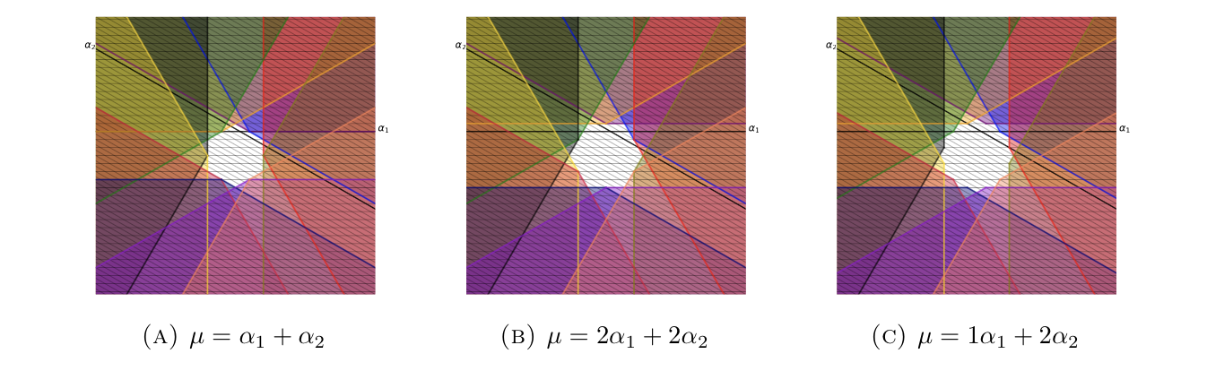
Figure 1. Weyl alternation diagrams of $\mathfrak{g}_{2}$ with a specified $\mu$.

In the present work, we consider the Lie algebra $\mathfrak{sl}_{4}(\mathbb{C})$ and we

1. give closed formulas for the $q$-analog of Kostant’s partition function for any weight $\xi$,

2. compute the Weyl alternation sets for every pair of integral weights $(\lambda,\mu)$,

3. illustrate the Weyl alternation diagrams when $\mu=0$ and $\lambda=a_{1}\alpha_{1}+a_{2}\alpha_{2}+a_{3}\alpha_{3}$ with $a_{1},a_{2},a_{3}\in\mathbb{N}$, as well as describe the empty region for a variety of weights $\mu$,

4. use (1) and (2) to give a closed formula for the $q$-analog of Kostant’s weight multiplicity formula for $\mathfrak{sl}_{4}(\mathbb{C})$, and

5. provide code for all of the above mentioned results, which can be found in the GitHub repository at https://github.com/melendezd/Weight-Multiplicities.

1.1. Statements of main results and some specializations

Throughout, we let $\alpha_{1}$, $\alpha_{2}$, and $\alpha_{3}$ denote the simple roots, and $\varpi_{1}$, $\varpi_{2}$, and $\varpi_{3}$ denote the fundamental weights of $\mathfrak{sl}_{4}(\mathbb{C})$. Harris, Rahmoeller, Schneider, and Simpson gave the following formula for the $q$-analog of Kostant’s partition function for the Lie algebra $\mathfrak{sl}_{4}(\mathbb{C})$.

Proposition 1 (Proposition 5.1 in [20]).

If $m,n,k\in\mathbb{N}$, then

$$\wp_{q}(m\alpha_{1}+n\alpha_{2}+k\alpha_{3})=\sum_{f=0}^{\min(m,n,k)}\;\sum_{d=0}^{\min(m-f,n-f)}\;\sum_{e=0}^{\min(n-d-f,k-f)}q^{m+n+k-2f-d-e}.$$

The formula in Proposition 1 can be readily implemented in a computer program. However, as $m,n,$ and $k$ grow, the runtime for this algorithm grows rapidly. This motivates our first result.

Theorem 1.

Let $m,n,k\in\mathbb{N}:=\{0,1,2,\ldots\}$ and $\xi=m\alpha_{1}+n\alpha_{2}+k\alpha_{3}$.

1. If $m,k\geq n$, then $\wp_{q}(\xi)=\sum_{i=m+k-n}^{m+n+k}(L+1)(L+(t\bmod 2)+1)q^{i}$ where $L=\min\left\{\left\lfloor\frac{t}{2}\right\rfloor,n-\left\lceil\frac{t}{2}\right\rceil\right\}$ and $t=m+n+k-i$.

2. If $m\geq n\geq k$, then $\wp_{q}(\xi)=\sum_{i=m}^{m+n+k}c_{i}q^{i}$ where

   $$c_{i}=\begin{cases}\frac{(L+1)(2k-2F_{2}+L+2)}{2}&\mbox{if}\ J<0\\ \frac{(L+1)(L+2)-F_{2}(F_{2}+1)-k(k-1)}{2}+F_{2}k+kL-F_{2}L+(k-F_{2})(t\bmod 2)&\mbox{if}\ 0\leq J\leq L\\ (L+1)(L+(t\bmod 2)+1)&\mbox{if}\ J>L\end{cases}$$

   with $t=m+n+k-i$, $F_{2}=\min\left\{\left\lfloor\frac{t}{2}\right\rfloor,k\right\}$, $J=k-F_{2}-(t\bmod 2)$, $F_{1}=\max\{t-n,0\}$, and $L=F_{2}-F_{1}$.

3. If $k\geq n\geq m$, then $\wp_{q}(\xi)=\sum_{i=k}^{m+n+k}c_{i}q^{i}$ where

   $$c_{i}=\begin{cases}\frac{(L+1)(2m-2F_{2}+L+2)}{2}&\mbox{if}\ J<0\\ \frac{(L+1)(L+2)-F_{2}(F_{2}+1)-m(m-1)}{2}+F_{2}m+mL-F_{2}L+(m-F_{2})(t\bmod 2)&\mbox{if}\ 0\leq J\leq L\\ (L+1)(L+(t\bmod 2)+1)&\mbox{if}\ J>L\end{cases}$$

   with $t=m+n+k-i$, $F_{2}=\min\left\{\left\lfloor\frac{t}{2}\right\rfloor,m\right\}$, $J=m-F_{2}-(t\bmod 2)$, $F_{1}=\max\{t-n,0\}$, and $L=F_{2}-F_{1}$.

4. If $n\geq m\geq k$, then $\wp_{q}(\xi)=\sum_{i=n}^{m+n+k}c_{i}q^{i}$ where $c_{i}=S_{1}-S_{2}+F_{2}-F_{1}+1$ and

   $$S_{1} =\begin{cases}(t-F_{2})(F_{2}+1)&\mbox{if}\ t-m<0\\ \frac{(t-m)(t-m+1)+F_{1}(F_{1}-1)-2F_{2}(F_{2}+1)+2m(t-m-F_{1}+1)+2t(F_{2}-t+m)}{2}&\mbox{if}\ 0\leq t-m\leq F_{2}\end{cases}$$

   $$S_{2} =\begin{cases}(t-k)(t-k-F_{1}+1)-\frac{(t-k)(t-k+1)-F_{1}(F_{1}-1)}{2}&\mbox{if}\ 0\leq t-k\leq F_{2}\\ (t-k)(F_{2}-F_{1}+1)-\frac{F_{2}(F_{2}+1)-F_{1}(F_{1}-1)}{2}&\mbox{if}\ t-k>F_{2}\\ 0&\mbox{if}\ t-k<0\end{cases}$$

   with $t=m+n+k-i$, $F_{1}=\max\{0,t-\min\{m+k,n\}\}$, and $F_{2}=\min\left\{\left\lfloor\frac{t}{2}\right\rfloor,k\right\}$.

5. If $n\geq k\geq m$, then $\wp_{q}(\xi)=\sum_{i=n}^{m+n+k}c_{i}q^{i}$ where $c_{i}=S_{1}-S_{2}+F_{2}-F_{1}+1$ and

   $$S_{1} =\begin{cases}(t-F_{2})(F_{2}+1)&\mbox{if}\ t-k<0\\ \frac{(t-k)(t-k+1)+F_{1}(F_{1}-1)-2F_{2}(F_{2}+1)+2k(t-k-F_{1}+1)+2t(F_{2}-t+k)}{2}&\mbox{if}\ 0\leq t-k\leq F_{2}\end{cases}$$

   $$S_{2} =\begin{cases}(t-m)(t-m-F_{1}+1)-\frac{(t-m)(t-m+1)-F_{1}(F_{1}-1)}{2}&\mbox{if}\ 0\leq t-m\leq F_{2}\\ (t-m)(F_{2}-F_{1}+1)-\frac{F_{2}(F_{2}+1)-F_{1}(F_{1}-1)}{2}&\mbox{if}\ t-m>F_{2}\\ 0&\mbox{if}\ t-m<0\end{cases}$$

   with $t=m+n+k-i$, $F_{1}=\max\{0,t-\min\{m+k,n\}\}$, and $F_{2}=\min\left\{\left\lfloor\frac{t}{2}\right\rfloor,m\right\}$.

Our proof of Theorem 1 counts restricted integer partitions with parts of multiple colors, thereby giving interesting connections between these types of partitions and vector partitions. Moreover, as mentioned above, we note that the runtime for computing $\wp_{q}(m\alpha_{1}+n\alpha_{2}+k\alpha_{3})$ for $60\leq m,n,k<70$ was $359$ms on average using an algorithm based on Proposition 1, while the same computations took less than $2$ms on average using the closed formulas in Theorem 1. In general, the runtime of an algorithm to compute each coefficient of $\wp_{q}(\xi)$ based on Proposition 1 grows at least linearly with $\wp(\xi)$, while the runtime of an algorithm using Theorem 1 remains constant. We also remark that evaluating the formulas in Theorem 1 at $q=1$ recovers formulas of De Loera and Sturmfels [7, Section 5], which we present below.

Corollary 1.

Let $m,n,k\in\mathbb{N}$ and $\xi=m\alpha_{1}+n\alpha_{2}+k\alpha_{3}$.

1. If $m,k\geq n$, then $\wp(\xi)=\frac{(n+1)(n+2)(n+3)}{6}$.

2. If $m\geq n\geq k$, then $\wp(\xi)=\frac{(k+1)(k+2)(k+3(n-k)+3)}{6}$.

3. If $k\geq n\geq m$, then $\wp(\xi)=\frac{(m+1)(m+2)(m+3(n-m)+3)}{6}$.

4. If $n\geq m\geq k$ and $n\geq m+k$, then $\wp(\xi)=\frac{(k+1)(k+2)(3m-k+3)}{6}$.

5. If $n\geq k\geq m$ and $n\geq m+k$, then $\wp(\xi)=\frac{(m+1)(m+2)(3k-m+3)}{6}$.

6. If $n\geq m\geq k$ and $m+k\geq n$, then

   $$\wp(\xi)=\frac{-2k^{3}-(m-n)^{2}(3+m-n)+3k^{2}(n-1)+2(3+2m+n)+k(5-3m^{2}-3(n-2)n+m(3+6n))}{6}.$$

7. If $n\geq k\geq m$ and $m+k\geq n$, then

   $$\wp(\xi)=\frac{-2m^{3}-(k-n)^{2}(3+k-n)+3m^{2}(n-1)+2(3+2k+n)+m(5-3k^{2}-3(n-2)n+k(3+6n))}{6}.$$

We note that the formula in [7, Item 4 (above Theorem 6.1 on page 14)] is missing a factor of $1/6$, which we correct in Corollary 1 parts (4) and (5). We also remark that in Corollary 1 there are 7 cases, while there are only 5 in Theorem 1. This is because part (5) in Theorem 1 encompasses cases (5) and (7) in Corollary 1, and part (4) in Theorem 1 encompasses cases (4) and (6) in Corollary 1.

Our second main result, Theorem 2 in Section 4, describes the Weyl alternation sets $\mathcal{A}(\lambda,\mu)$ for any pair of integral weights $\lambda$ and $\mu$. This result establishes that there are a total of 195 distinct Weyl alternation sets and that the maximum cardinality among all Weyl alternation sets is $6$. Given the length of Theorem 2 we defer its statement until Section 4. To illustrate Theorem 2, we consider $\lambda$ in the nonnegative octant of the root lattice of $\mathfrak{sl}_{4}(\mathbb{C})$ and obtain the following result.

Corollary 2.

If $\mu=0$ and $\lambda=(2x-y)\varpi_{1}+(2y-x-z)\varpi_{2}+(2z-y)\varpi_{3}$ with $x,y,z,2x-y,2y-x-z,2z-y\in\mathbb{N}$, then $\lambda$ is in the nonnegative integral root lattice $\mathbb{N}\alpha_{1}\oplus\mathbb{N}\alpha_{2}\oplus\mathbb{N}\alpha_{3}$ and

1. $\mathcal{A}_{1}:=\mathcal{A}(\lambda,0)=\{1\}$ if $\lambda=0$,

2. $\mathcal{A}_{2}:=\mathcal{A}(\lambda,0)=\{1,s_{2}\}$ if $x+z-y-1\in\mathbb{N}$, $-1<x-y<2$, and $-1<z-y<2$,

3. $\mathcal{A}_{3}:=\mathcal{A}(\lambda,0)=\{1,s_{2},s_{3}\}$ if $x+z-y-1,y-z-1\in\mathbb{N}$ , $x-y-2\notin\mathbb{N}$, and $-1<x-y<2$,

4. $\mathcal{A}_{4}:=\mathcal{A}(\lambda,0)=\{1,s_{1},s_{2}\}$ if $y-x-1,x+z-y-1\in\mathbb{N}$, $z-x-2\notin\mathbb{N}$, and $-1<z-y<2$,

5. $\mathcal{A}_{5}:=\mathcal{A}(\lambda,0)=\{1,s_{2},s_{3},s_{2}s_{3}\}$ if $x-z-2,x+z-y-1,y-z-1\in\mathbb{N}$, and $-1<x-y<2$,

6. $\mathcal{A}_{6}:=\mathcal{A}(\lambda,0)=\{1,s_{1},s_{3},s_{3}s_{1}\}$ if $y-x-1,y-z-1\in\mathbb{N}$, $z+z-y-1\notin\mathbb{N}$, and $-2<x-z<2$,

7. $\mathcal{A}_{7}:=\mathcal{A}(\lambda,0)=\{1,s_{1},s_{2},s_{2}s_{1}\}$ if $y-x-1,z-x-2,x+z-y-1\in\mathbb{N}$, and $-1<z-y<2$,

8. $\mathcal{A}_{8}:=\mathcal{A}(\lambda,0)=\{1,s_{1},s_{2},s_{3},s_{3}s_{1}\}$ if $x+z-y-1,y-x-1,y-z-1\in\mathbb{N}$, and $-2<x-z<2$,

9. $\mathcal{A}_{9}:=\mathcal{A}(\lambda,0)=\{1,s_{1},s_{2},s_{3},s_{2}s_{3},s_{3}s_{1}\}$ if $x+z-y-1,y-x-1,x-z-2,y-z-1\in\mathbb{N}$,

10. $\mathcal{A}_{10}:=\mathcal{A}(\lambda,0)=\{1,s_{1},s_{2},s_{3},s_{2}s_{1},s_{3}s_{1}\}$ if $x+z-y-1,y-x-1,z-x-2,y-z-1\in\mathbb{N}$,

11. $\mathcal{A}_{11}:=\mathcal{A}(\lambda,0)=\{1,s_{2},s_{3},s_{2}s_{3},s_{3}s_{2},s_{2}s_{3}s_{2}\}$ if $x+z-y-1,x-z-2,x-y-2,y-z-1\in\mathbb{N}$,

12. $\mathcal{A}_{12}:=\mathcal{A}(\lambda,0)=\{1,s_{1},s_{2},s_{1}s_{2},s_{2}s_{1},s_{1}s_{2}s_{1}\}$ if $x+z-y-1,z-y-2,y-z-1,z-x-1\in\mathbb{N}$,

13. $\mathcal{A}(\lambda,0)=\emptyset$, otherwise.

In Figure 2, we illustrate the 12 nonempty Weyl alternation sets given by Corollary 2. In these figures, the axes are the nonnegative real span of the simple roots $\alpha_{1}$ (in red), $\alpha_{2}$ (in green), and $\alpha_{3}$ (in blue). For each $1\leq i\leq 12$, the colored vertices within each particular subfigure depict the a set of weights whose Weyl alternation set is indicated in the caption.

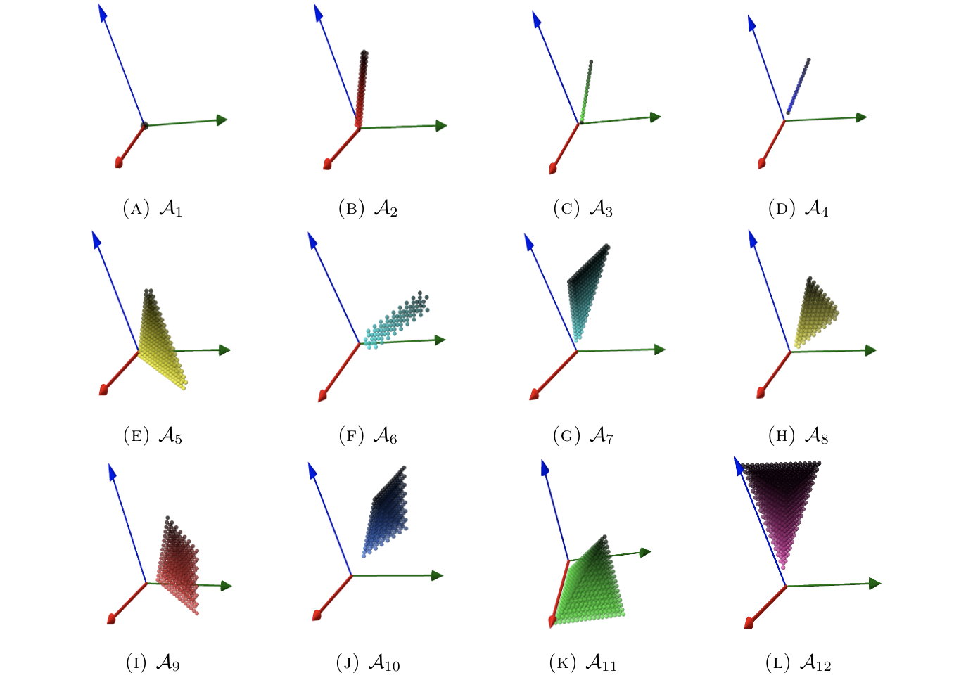
Figure 2. The Weyl alternation diagrams of Corollary 2.

In Figure 3, we illustrate some of the possible behavior of the central empty region for the Lie algebra $\mathfrak{sl}_{4}(\mathbb{C})$. For a fixed $\mu=c_{1}\alpha_{1}+c_{2}\alpha_{2}+c_{3}\alpha_{3}$, with $c_{1},c_{2},c_{3}\in\mathbb{N}$, the colored vertices in Figure 3 denote the weights $\lambda=m\varpi_{1}+n\varpi_{2}+k\varpi_{2}$, with $m,n,k\in\mathbb{Z}$, for which $\mathcal{A}(\lambda,\mu)=\emptyset$. Such regions are completely described by Theorem 2. Thus, Theorem 2 answers [17, Question 5.1], by giving the Weyl alternation diagrams of $\mathfrak{sl}_{4}(\mathbb{C})$ along with a description of how the empty region diagrams change as the weight $\mu$ changes.

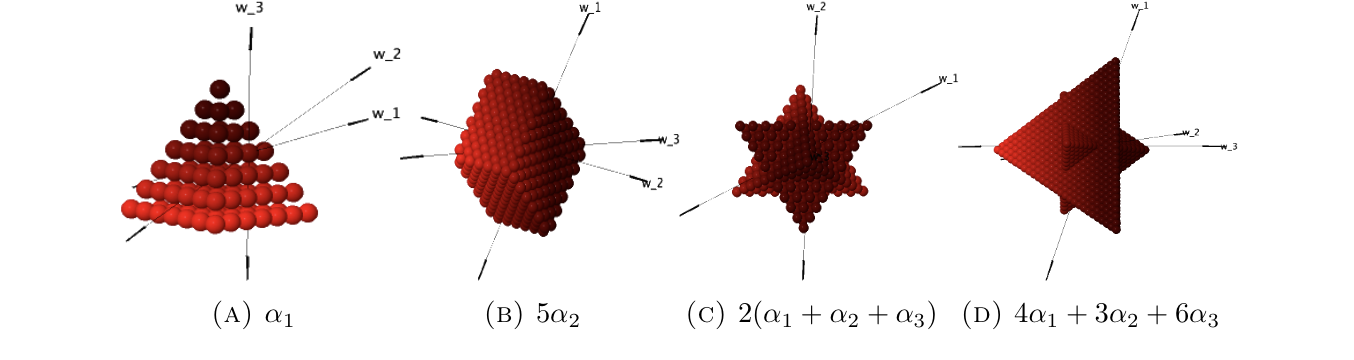
Figure 3. Various empty regions associated to $\mathfrak{sl}_{4}(\mathbb{C})$ with a fixed weight $\mu$.

Our last main result presents a closed formula for the $q$-analog of Kostant’s weight multiplicity formula for the Lie algebra $\mathfrak{sl}_{4}(\mathbb{C})$ for dominant integral weight $\lambda$ and $\mu$. This restriction is motivated by the fact that the weights which lie on the nonnegative octant of the fundamental weight lattice are in correspondence with the finite-dimensional irreducible representations of $\mathfrak{sl}_{4}(\mathbb{C})$. Theorem 3 utilizes the closed formulas for the $q$-analog of Kostant’s partition function given by Theorem 1 and the Weyl alternation sets $\mathcal{A}(\lambda,\mu)$ given by Theorem 2.

Theorem 3.

Let $\lambda=m\varpi_{1}+n\varpi_{2}+k\varpi_{3}$ and $\mu=c_{1}\varpi_{1}+c_{2}\varpi_{2}+c_{3}\varpi_{3}$ with $m,n,k,c_{1},c_{2},c_{3}\in\mathbb{N}$. If $x=\frac{3m+2n+k-3c_{1}-2c_{2}-c_{3}}{4}$, $y=\frac{m+2n+k-c_{1}-2c_{2}-c_{3}}{2}$, and $z=\frac{m+2n+3k-c_{1}-2c_{2}-3c_{3}}{4}$, then

$$m_{q}(\lambda,\mu)=\begin{cases}Z_{1}-Z_{11}-Z_{3}+Z_{5}+Z_{10}-Z_{7}&P_{1},Q_{1},R_{1},Q_{6},R_{4},Q_{5},R_{3}\in\mathbb{N}\ \text{and}\ P_{4},P_{3}\notin\mathbb{N}\\ Z_{1}-Z_{6}-Z_{3}+Z_{4}+Z_{8}-Z_{2}&P_{1},Q_{1},R_{1},P_{4},Q_{6},P_{3},Q_{4}\in\mathbb{N}\ \text{and}\ R_{4},R_{3}\notin\mathbb{N}\\ Z_{1}-Z_{6}-Z_{11}-Z_{3}+Z_{8}+Z_{9}&P_{1},Q_{1},R_{1},P_{4},R_{4},Q_{6},Q_{4}\in\mathbb{N}\ \text{and}\ P_{3},Q_{5},R_{3}\notin\mathbb{N}\\ Z_{1}-Z_{6}-Z_{11}-Z_{3}+Z_{9}+Z_{5}&P_{1},Q_{1},R_{1},P_{4},Q_{6},R_{4},Q_{5}\in\mathbb{N}\ \text{and}\ P_{3},Q_{4},R_{3}\notin\mathbb{N}\\ Z_{1}-Z_{6}-Z_{11}-Z_{3}+Z_{9}&P_{1},Q_{1},R_{1},P_{4},Q_{6},R_{4}\in\mathbb{N}\ \text{and}\ P_{3},Q_{4},Q_{5},R_{3}\notin\mathbb{N}\\ Z_{1}-Z_{11}-Z_{3}+Z_{5}&P_{1},Q_{1},R_{1},Q_{6},R_{4},Q_{5}\in\mathbb{N}\ \text{and}\ P_{4},P_{3},R_{3}\notin\mathbb{N}\\ Z_{1}-Z_{6}-Z_{3}+Z_{9}&P_{1},Q_{1},R_{1},P_{4},R_{4}\in\mathbb{N}\ \text{and}\ Q_{6},Q_{4},Q_{5}\notin\mathbb{N}\\ Z_{1}-Z_{6}-Z_{11}+Z_{8}&P_{1},Q_{1},R_{1},P_{4},Q_{6},Q_{4}\in\mathbb{N}\ \text{and}\ R_{4},P_{3},R_{3}\notin\mathbb{N}\\ Z_{1}-Z_{11}-Z_{3}&P_{1},Q_{1},R_{1},Q_{6},R_{4}\in\mathbb{N}\ \text{and}\ P_{4},P_{3},Q_{5},R_{3}\notin\mathbb{N}\\ Z_{1}-Z_{6}-Z_{11}&P_{1},Q_{1},R_{1},P_{4},Q_{6}\in\mathbb{N}\ \text{and}\ R_{4},P_{3},Q_{4},R_{3}\notin\mathbb{N}\\ Z_{1}-Z_{3}&P_{1},Q_{1},R_{1},R_{4}\in\mathbb{N}\ \text{and}\ Q_{6},P_{4},Q_{5}\notin\mathbb{N}\ \text{and}\ (P_{3}\notin\mathbb{N}\ \text{or}\ Q_{4}\notin\mathbb{N})\\ Z_{1}-Z_{11}&P_{1},Q_{1},R_{1},Q_{6}\in\mathbb{N}\ \text{and}\ P_{4},R_{4},R_{3},P_{3}\notin\mathbb{N}\\ Z_{1}-Z_{6}&P_{1},Q_{1},R_{1},P_{4}\in\mathbb{N}\ \text{and}\ Q_{6},R_{4},Q_{4}\notin\mathbb{N}\ \text{and}\ (Q_{5}\notin\mathbb{N}\ \text{or}\ R_{3}\notin\mathbb{N})\\ Z_{1}&P_{1},Q_{1},R_{1}\in\mathbb{N}\ \text{and}\ R_{4},P_{4},Q_{6}\notin\mathbb{N}\ \text{and}\ (P_{3}\notin\mathbb{N}\ \text{or}\ Q_{4}\notin\mathbb{N})\\ &\text{and}\ (Q_{5}\notin\mathbb{N}\ \text{or}\ R_{3}\notin\mathbb{N})\\ 0&\textnormal{otherwise,}\end{cases}$$

where

$$Z_{1}= \wp_{q}(1(\lambda+\rho)-(\rho+\mu))=\wp_{q}(P_{1}\alpha_{1}+Q_{1}\alpha_{2}+R_{1}\alpha_{3})$$

$$Z_{2}= \wp_{q}(s_{1}s_{2}s_{1}(\lambda+\rho)-(\rho+\mu))=\wp_{q}(P_{3}\alpha_{1}+Q_{4}\alpha_{2}+R_{1}\alpha_{3})$$

$$Z_{3}= \wp_{q}(s_{3}(\lambda+\rho)-(\rho+\mu))=\wp_{q}(P_{1}\alpha_{1}+Q_{1}\alpha_{2}+R_{4}\alpha_{3})$$

$$Z_{4}= \wp_{q}(s_{1}s_{2}(\lambda+\rho)-(\rho+\mu))=\wp_{q}(P_{3}\alpha_{1}+Q_{6}\alpha_{2}+R_{1}\alpha_{3})$$

$$Z_{5}= \wp_{q}(s_{2}s_{3}(\lambda+\rho)-(\rho+\mu))=\wp_{q}(P_{1}\alpha_{1}+Q_{5}\alpha_{2}+R_{4}\alpha_{3})$$

$$Z_{6}= \wp_{q}(s_{1}(\lambda+\rho)-(\rho+\mu))=\wp_{q}(P_{4}\alpha_{1}+Q_{1}\alpha_{2}+R_{1}\alpha_{3})$$

$$Z_{7}= \wp_{q}(s_{2}s_{3}s_{2}(\lambda+\rho)-(\rho+\mu))=\wp_{q}(P_{1}\alpha_{1}+Q_{5}\alpha_{2}+R_{3}\alpha_{3})$$

$$Z_{8}= \wp_{q}(s_{2}s_{1}(\lambda+\rho)-(\rho+\mu))=\wp_{q}(P_{4}\alpha_{1}+Q_{4}\alpha_{2}+R_{1}\alpha_{3})$$

$$Z_{9}= \wp_{q}(s_{3}s_{1}(\lambda+\rho)-(\rho+\mu))=\wp_{q}(P_{4}\alpha_{1}+Q_{1}\alpha_{2}+R_{4}\alpha_{3})$$

$$Z_{10}= \wp_{q}(s_{3}s_{2}(\lambda+\rho)-(\rho+\mu))=\wp_{q}(P_{1}\alpha_{1}+Q_{6}\alpha_{2}+R_{3}\alpha_{3})$$

$$Z_{11}= \wp_{q}(s_{2}(\lambda+\rho)-(\rho+\mu))=\wp_{q}(P_{1}\alpha_{1}+Q_{6}\alpha_{2}+R_{1}\alpha_{3})$$

and $P_{1}=x$, $P_{3}=-c_{1}-c_{2}-y+z-2$, $P_{4}=-c_{1}-x+y-1$, $Q_{1}=y$, $Q_{4}=-c_{1}-c_{2}-x+z-2$, $Q_{5}=-c_{2}-c_{3}+x-z-2$, $Q_{6}=-c_{2}+x-y+z-1$, $R_{1}=z$, $R_{3}=-c_{2}-c_{3}+x-y-2$, and $R_{4}=-c_{3}+y-z-1$.

For each $1\leq i\leq 11$, the formula for $Z_{i}$ given in Theorem 3 is obtained by an application of Theorem 1, see Appendix B for the details of this. By evaluating $q=1$ in Theorem 3 we give a formula for the multiplicity of the weight $\mu$ in the highest weight representation $L(\lambda)$ of $\mathfrak{sl}_{4}(\mathbb{C})$, with highest dominant integral weight $\lambda$.

Outline of the Paper

The remainder of the manuscript is organized as follows. Section 2 provides all of the necessary background on the Lie algebra $\mathfrak{sl}_{4}(\mathbb{C})$ in order to make our approach precise. Section 3 establishes Theorem 1 using a combinatorial approach related to integer paritions. Section 4 presents all of the results associated to the Weyl alternation sets and Weyl alternation diagrams. Section 5 establishes Theorem 3. We end with Section 6 where we provide a few directions for future research. In particular, we ask about further connections between Kostant’s partition function and restricted colored integer partitions.

2. Background

In this section we provide definitions needed to make our approach precise throughout the following sections. We follow the notation used in [8].

The Lie algebra $\mathfrak{sl}_{4}(\mathbb{C})$ consists of traceless $4\times 4$ complex-valued matrices. We will consider the Cartan subalgebra, $\mathfrak{h}$ of $\mathfrak{sl}_{4}(\mathbb{C})$, consisting of the diagonal matrices of $\mathfrak{sl}_{4}(\mathbb{C})$. For $i=1,2,3$ let $\alpha_{i}=e_{i}-e_{i+1}$, where $e_{1},e_{2},e_{3},e_{4}$ denote the standard basis vectors of $\mathbb{R}^{4}$. Then the set $\Delta=\{\alpha_{1},\alpha_{2},\alpha_{3}\}$ is a set of simple roots and $\Phi^{+}=\{\alpha_{1},\alpha_{2},\alpha_{3},\alpha_{1}+\alpha_{2},\alpha_{2}+\alpha_{3},\alpha_{1}+\alpha_{2}+\alpha_{3}\}$ is the corresponding set of positive roots of $\mathfrak{sl}_{4}(\mathbb{C})$. Figure 4 gives a geometry-preserving projection of the root system of $\mathfrak{sl}_{4}(\mathbb{C})$ into $\mathbb{R}^{3}$. The fundamental weights of $\mathfrak{sl}_{4}(\mathbb{C})$ are

(2) $$\varpi_{1} =\frac{1}{4}(3\alpha_{1}+2\alpha_{2}+\alpha_{3}),\qquad\varpi_{2}=\frac{1}{2}(\alpha_{1}+2\alpha_{2}+\alpha_{3}),\qquad\varpi_{3}=\frac{1}{4}(\alpha_{1}+2\alpha_{2}+3\alpha_{3}).$$

Hence, $\rho=\frac{1}{2}\sum_{\alpha\in\Phi^{+}}\alpha=\varpi_{1}+\varpi_{2}+\varpi_{3}=\frac{1}{2}(3\alpha_{1}+4\alpha_{2}+3\alpha_{3})$.

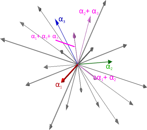
Figure 4. Root system of $\mathfrak{sl}_{4}(\mathbb{C})$.

The Weyl group of $\mathfrak{sl}_{4}(\mathbb{C})$ is isomorphic to the symmetric group $\mathfrak{S}_{4}$ and its generators are $s_{1}$, $s_{2}$, and $s_{3}$ which act as reflections across hyperplanes orthogonal to the simple roots $\alpha_{1},\alpha_{2},\alpha_{3}$, respectively. In particular for $1\leq i\leq 3$ we have that

$$s_{i}(\alpha_{j})=\begin{cases}-\alpha_{j}&\mbox{if $i=j$}\\ \alpha_{i}+\alpha_{j}&\mbox{if $|i-j|=1$}\\ \alpha_{j}&\mbox{if $|i-j|>1$}\end{cases}\qquad\mbox{and}\qquad s_{i}(\varpi_{j})=\begin{cases}\varpi_{j}&\mbox{if $i\neq j$}\\ \varpi_{j}-\alpha_{j}&\mbox{if $i=j$}.\end{cases}$$

We conclude this section with the following result which will be important when computing Weyl alternation sets in Section 4.

Lemma 1.

Let $\lambda=m\varpi_{1}+n\varpi_{2}+k\varpi_{3}$, with $m,n,k\in\mathbb{Z}$. Then $\lambda=c_{1}{\alpha_{1}}+c_{2}\alpha_{2}+c_{3}\alpha_{3}$, for some $c_{1},c_{2},c_{3}\in\mathbb{Z}$ if and only if $m=2x-y,n=2y-z-x$ and $k=2z-y$ where $x,y,z\in\mathbb{Z}.$

Proof.

First, we prove the forward direction. Let $\lambda=m\varpi_{1}+n\varpi_{2}+k\varpi_{3}$, with $m,n,k\in\mathbb{Z}.$ By (2) we write $\lambda$ as

$$\lambda =\frac{m}{4}(3\alpha_{1}+2\alpha_{2}+\alpha_{3})+\frac{n}{2}(\alpha_{1}+2\alpha_{2}+\alpha_{3})+\frac{k}{4}(\alpha_{1}+2\alpha_{2}+3\alpha_{3})$$

$$=\Big{(}\frac{3m+2n+k}{4}\Big{)}\alpha_{1}+\Big{(}\frac{2m+4n+2k}{4}\Big{)}\alpha_{2}+\Big{(}\frac{m+2n+3k}{4}\Big{)}\alpha_{3}.$$

In order for $\lambda=c_{1}{\alpha_{1}}+c_{2}\alpha_{2}+c_{3}\alpha_{3}$ for some $c_{1},c_{2},c_{3}\in\mathbb{Z}$, it must be that

(3) $$3m+2n+k =4x$$

(4) $$2m+4n+2k =4y$$

(5) $$m+2n+3k =4z$$

for some $x,y,z\in\mathbb{Z}.$ Then, from (3), we know $k=4x-3m-2n$, and so substituting into (4) and simplifying yields $m=2x-y$. Similarly, solving for $m$ in (5) shows $m=4z-2n-3k$. Substituting this into equation (4) and simplifying yields $k=2z-y$. Lastly, substituting $m=2x-y$ and $k=2z-y$ into (3) establishes that $n=2y-x-z$, as desired.

To prove the backwards direction, let $\lambda=m\omega_{1}+n\omega_{2}+k\omega_{3}$ and assume

(6) $$m =2x-y$$

(7) $$n =2y-z-x$$

(8) $$k =2z-y$$

where $x,y,z\in\mathbb{Z}$, By (2) we can write $\lambda$ in terms of the simple roots as

(9) $$\lambda =\Big{(}\frac{3m+2n+k}{4}\Big{)}\alpha_{1}+\Big{(}\frac{2m+4n+2k}{4}\Big{)}\alpha_{2}+\Big{(}\frac{m+2n+3k}{4}\Big{)}\alpha_{3}.$$

Substituting (6), (7), and (8) into (9), gives $\lambda=x\alpha_{1}+y\alpha_{2}+z\alpha_{3}$, which completes the proof. ∎

3. Formulas for the $q$-analog of Kostant’s partition function

In this section we establish Theorem 1, which generalizes the formulas of De Loera and Sturmfels for the Kostant’s partition function of $\mathfrak{sl}_{4}(\mathbb{C})$ to its $q$-analog [7]. Our general strategy is to reduce the problem of counting partitions of a weight with a fixed number of parts to the problem of counting restricted partitions of an integer with parts drawn from a multiset of natural numbers. We begin with the following definition.

Definition 1.

Let $t\in\mathbb{N}$, and let $\mathcal{M}$ be a multiset with elements from $\mathbb{N}$. Then an $\mathcal{M}$-partition of $t$ is a sequence of natural numbers $(a_{m})_{m\in\mathcal{M}}$ such that $\sum_{m\in\mathcal{M}}m\cdot a_{m}=t$.

When working with elements of a multiset we associate a “color” to elements with multiplicity greater than one so that we may distinguish them. For more on colored partitions, restricted colored partitions, and their properties, see [4, 5, 21, 22]. The following example illustrates Definition 1 in the case when $\mathcal{M}=\{1,1,2\}$.

Example 1.

For ease of distinguishing between the multiple $1$’s we let $\mathcal{M}$ be the multiset $\mathcal{M}=\{{\color[rgb]{1,0,0}1_{r}},{\color[rgb]{0,0,1}1_{b}},2\}$. Then the distinct $\mathcal{M}$-partitions of $4$ are ${\color[rgb]{1,0,0}1_{r}}+{\color[rgb]{1,0,0}1_{r}}+2$, ${\color[rgb]{1,0,0}1_{r}}+{\color[rgb]{0,0,1}1_{b}}+2$, ${\color[rgb]{0,0,1}1_{b}}+{\color[rgb]{0,0,1}1_{b}}+2$, ${\color[rgb]{1,0,0}1_{r}}+{\color[rgb]{1,0,0}1_{r}}+{\color[rgb]{1,0,0}1_{r}}+{\color[rgb]{1,0,0}1_{r}}$, ${\color[rgb]{0,0,1}1_{b}}+{\color[rgb]{1,0,0}1_{r}}+{\color[rgb]{1,0,0}1_{r}}+{\color[rgb]{1,0,0}1_{r}}$, ${\color[rgb]{0,0,1}1_{b}}+{\color[rgb]{0,0,1}1_{b}}+{\color[rgb]{1,0,0}1_{r}}+{\color[rgb]{1,0,0}1_{r}}$, ${\color[rgb]{0,0,1}1_{b}}+{\color[rgb]{0,0,1}1_{b}}+{\color[rgb]{0,0,1}1_{b}}+{\color[rgb]{1,0,0}1_{r}}$, ${\color[rgb]{0,0,1}1_{b}}+{\color[rgb]{0,0,1}1_{b}}+{\color[rgb]{0,0,1}1_{b}}+{\color[rgb]{0,0,1}1_{b}}$, and $2+2$.

Next, we establish a bijection between vector partitions with a fixed number of parts and restricted colored integer partitions, a result which will be central to the remainder of this paper.

Proposition 2.

Let $m,n,k,i\in\mathbb{N}$, and let $\xi=m\alpha_{1}+n\alpha_{2}+k\alpha_{3}$. Then the number of ways to express $\xi$ as a sum of exactly $i$ positive roots is equal to the number of $\{{\color[rgb]{1,0,0}1_{r}},{\color[rgb]{0,0,1}1_{b}},2\}$-partitions $d\cdot{\color[rgb]{1,0,0}1_{r}}+e\cdot{\color[rgb]{0,0,1}1_{b}}+f\cdot 2$ of $t:=m+n+k-i$ that satisfy

1. $d+f\leq m$,

2. $d+e+f\leq n$, and

3. $e+f\leq k$.

Proof.

Let $X$ denote the set of partitions of $\xi$ using positive roots, where $(a,b,c,d,e,f)$ corresponds to the partition $\xi=a\alpha_{1}+b\alpha_{2}+c\alpha_{3}+d(\alpha_{1}+\alpha_{2})+e(\alpha_{2}+\alpha_{3})+f(\alpha_{1}+\alpha_{2}+\alpha_{3})$. Let $Y$ denote the set of $\{{\color[rgb]{1,0,0}1_{r}},{\color[rgb]{0,0,1}1_{b}},2\}$-partitions of $t$ satisfying (i)-(iii), where the tuple $(d,e,f)$ corresponds to the partition $t=d\cdot{\color[rgb]{1,0,0}1_{r}}+e\cdot{\color[rgb]{0,0,1}1_{b}}+f\cdot 2$. We define a function $F:X\to Y$ which is given by $(a,b,c,d,e,f)\mapsto(d,e,f)$.

To prove that $F$ is well-defined, let $p=(a,b,c,d,e,f)$ be a partition of $\xi$. Then the image of this partition under $F$ is the partition $d\cdot{\color[rgb]{1,0,0}1_{r}}+e\cdot{\color[rgb]{0,0,1}1_{b}}+f\cdot 2$. First, note that we can expand and combine terms to find that $a\alpha_{1}+b\alpha_{2}+c\alpha_{3}+d(\alpha_{1}+\alpha_{2})+e(\alpha_{2}+\alpha_{3})+f(\alpha_{1}+\alpha_{2}+\alpha_{3})\\ =\ (a+d+f)\alpha_{1}+(b+d+e+f)\alpha_{2}+(c+e+f)\alpha_{3}$.

Comparing the coefficients of $\xi=m\alpha_{1}+n\alpha_{2}+k\alpha_{3}$ with the coefficients above, it follows that

$$a=m-d-f,\qquad b=n-d-e-f,\qquad c=k-e-f,$$

and so our partition is actually $(m-d-f,n-d-e-f,k-e-f,d,e,f)$. The number of parts in $p$ is $a+b+c+d+e+f=m+n+k-d-e-2f$. Hence, as defined above, we have that $t=d+e+2f$, and so $F(p)=(d,e,f)$ is indeed a $\{{\color[rgb]{1,0,0}1_{r}},{\color[rgb]{0,0,1}1_{b}},2\}$-partition of $t$.

Since $p\in X$, we have by definition that each of its components are nonnegative integers. Thus, $a,b,c\geq 0$ imply

$$d+f\leq m,\qquad d+e+f\leq n\\ \qquad e+f\leq k.$$

Thus, $(d,e,f)$ satisfies (i)-(iii) and is also a $\{{\color[rgb]{1,0,0}1_{r}},{\color[rgb]{0,0,1}1_{b}},2\}$ partition of $t$ and so is in $Y$.

Next to show that $F$ is a bijection, consider $G:Y\to X$ given by

$$(d,e,f)\mapsto(m-d-f,n-d-e-f,k-e-f,d,e,f).$$

A similar argument to the one above will show that $G$ is well defined and it is straightforward to check that $G$ is the inverse of $F$. It follows that $F$ is a bijection, and so $|X|=|Y|$, as desired. ∎

In the following subsections, we give closed formulas for $\wp_{q}(m\alpha_{1}+n\alpha_{2}+k\alpha_{3})$ in terms of $m$, $n$, and $k$ based on the following conditions:

1. $m,k\geq n$,

2. $m\geq n\geq k$,

3. $k\geq n\geq m$,

4. $n\geq m\geq k$, and

5. $n\geq k\geq m$.

As is standard, whenever a lower index of a sum is larger than the upper index, the sum is zero.

In Subsections 3.1-3.3, we apply Proposition 2 to determine closed formulas for $\wp_{q}$ in cases (1), (2), and (4). In each case, we determine the minimum number of parts that a partition of $\xi=m\alpha_{1}+n\alpha_{2}+k\alpha_{3}$ may have, giving us the lowest and highest powers of $q$ in $\wp_{q}(\xi)$. In general, note that the partition of the vector $m\alpha_{1}+n\alpha_{2}+k\alpha_{3}$ with the maximum number of parts is the partition $(m,n,k,0,0,0)$, which has $m+n+k$ parts.
In Subsection 3.4, we then exploit a symmetry in the root system for $\mathfrak{sl}_{4}(\mathbb{C})$ to find closed formulas for cases (3) and (5) using the closed formulas from cases (2) and (4), respectively.

3.1. Proof of Theorem 1, Part (1)

Lemma 2.

Let $m,n,k,t\in\mathbb{N}$ be such that $m,k\geq n$. The number of $\{{\color[rgb]{1,0,0}1_{r}},{\color[rgb]{0,0,1}1_{b}},2\}$-partitions of $t$ of the form $d\cdot{\color[rgb]{1,0,0}1_{r}}+e\cdot{\color[rgb]{0,0,1}1_{b}}+f\cdot 2$ with $d,e,f\in\mathbb{N}$ that satisfy

1. $d+f\leq m$,

2. $d+e+f\leq n$, and

3. $e+f\leq k$

is equal to

(10) $$\sum_{f=F_{1}}^{F_{2}}\sum_{d=D_{1}}^{D_{2}}1,$$

where $D_{1}=0,D_{2}=t-2f,F_{1}=\max\{0,t-n\},$ and $F_{2}=\left\lfloor\frac{t}{2}\right\rfloor.$

Proof.

We wish to show that if $d,e,f\in\mathbb{N}$ are such that $d+e+2f=t$, then (i)-(iii) hold if, and only if $D_{1}\leq d\leq D_{2}$ and $F_{1}\leq f\leq F_{2}$.

We begin by proving the converse direction. Assume $D_{1}\leq d\leq D_{2}$ and $F_{1}\leq f\leq F_{2}$.

For the inequality in (ii), note that since $f\geq F_{1}\geq t-n$, we get $t-n\leq f$. Then, by substituting $t=d+e+2f$, we get the desired inequality, $d+e+f\leq n$. Using this result, the fact that $m,k\geq n$, and $e,d\geq 0$ the other two inequalities follow. To obtain the inequality in (i), we have $d\leq n-e-f\leq n-f$, so $d+f\leq n\leq m$. To obtain the inequality in (iii), observe that $d+e+f\leq n$ implies $e\leq n-d-f\leq n-f$. Thus, $e+f\leq n\leq k$.

We now prove the forward direction. Assume (i)-(iii) hold.

We first show that $D_{1}\leq d\leq D_{2}$. Observe that $d\in\mathbb{N}$ and so $D_{1}=0\leq d.$ Now, from $t=d+e+2f,$ we have that $d=t-e-2f\leq t-2f=D_{2}$. Therefore, $D_{1}\leq d\leq D_{2}$.

We next show that $F_{1}\leq f\leq F_{2}$. Since $d+e+f\leq n$ and $t=d+e+2f$, we have $t-f=d+e+2f-f=d+e+f\leq n$, which implies that $t-n\leq f$. Furthermore, $f\in\mathbb{N}$ means that $0\leq f$. Therefore, $F_{1}=\max\{0,t-n\}\leq f$. Now, by definition, we have that $2f=t-d-e\leq t$. Since $f\in\mathbb{N}$, we have that $f\leq\left\lfloor\frac{t}{2}\right\rfloor=F_{2}$. Hence, $F_{1}\leq f\leq F_{2}.$

We have proved that if $d,e,f\in\mathbb{N}$ such that $d+e+2f=t,$ then (i)-(iii) hold if, and only if $D_{1}\leq d\leq D_{2}$ and $F_{1}\leq f\leq F_{2}$. Since $e$ is determined by $d$ and $f,$ it then follows that the number of $\{{\color[rgb]{1,0,0}1_{r}},{\color[rgb]{0,0,1}1_{b}},2\}$-partitions of $t$ satisfying (i)-(iii) is the sum in (10). ∎

We now establish part (1) of Theorem 1, which we restate below for ease of reference.

Proposition 3.

If $m,n,k\in\mathbb{N}$ satisfy $m,k\geq n$, then

$$\wp_{q}(m\alpha_{1}+n\alpha_{2}+k\alpha_{3})=\sum_{i=m+k-n}^{m+n+k}(L+1)(L+(t\bmod 2)+1)q^{i},$$

where $L=\min\left\{\left\lfloor\frac{t}{2}\right\rfloor,n-\left\lceil\frac{t}{2}\right\rceil\right\}$ and $t=m+n+k-i$.

Proof.

First, note that the maximum number of parts among all partitions of $\xi$ is $m+n+k$. To find the minimum number of parts among all partitions of $\xi$, we note that in a partition of $\xi$, we can use $\alpha_{1}+\alpha_{2}+\alpha_{3}$ at most $n$ times since $m,k\geq n$. Afterwards, we cannot use $\alpha_{1}+\alpha_{2}$ nor $\alpha_{2}+\alpha_{3}$ since $n(\alpha_{1}+\alpha_{2}+\alpha_{3})$ already contains the term $n\alpha_{2}$. Thus, we obtain a partition

$$\xi=(m-n)\alpha_{1}+(k-n)\alpha_{3}+n(\alpha_{1}+\alpha_{2}+\alpha_{3}),$$

with the minimum number of parts: $(m-n)+(k-n)+n=m+k-n$.

By Proposition 2, we know that for $i\in\mathbb{N}$, the number of vector partitions of $\xi$ with $i$ parts is equal to the number of $\{{\color[rgb]{1,0,0}1_{r}},{\color[rgb]{0,0,1}1_{b}},2\}$-partitions of $t=m+n+k-i$ that satisfy (i)-(iii). Lemma 2 then tells us that the number of such partitions of $t$ is

$$\sum_{f=\max\{0,t-n\}}^{\left\lfloor\frac{t}{2}\right\rfloor}\sum_{d=0}^{t-2f}1.$$

Thus, the number of partitions of $\xi$ using exactly $i$ positive roots is

$$\sum_{f=\max\{0,t-n\}}^{\left\lfloor\frac{t}{2}\right\rfloor}\sum_{d=0}^{t-2f}1 =\sum_{f=\max\{0,t-n\}}^{\left\lfloor\frac{t}{2}\right\rfloor}(t-2f+1).$$

Reindexing using $j=\left\lfloor\frac{t}{2}\right\rfloor-f$ and letting $L=\left\lfloor\frac{t}{2}\right\rfloor-\max\{0,t-n\}$, this sum becomes

$$\sum_{j=0}^{L}\left[t-2\left(\left\lfloor\frac{t}{2}\right\rfloor-j\right)+1\right] =\sum_{j=0}^{L}(2j+(t\bmod 2)+1)=(L+1)(L+(t\bmod 2)+1).$$

Finally, we simplify $L$:

$$L =\left\lfloor\frac{t}{2}\right\rfloor-\max\{0,t-n\}=\min\left\{\left\lfloor\frac{t}{2}\right\rfloor,n-\left(t-\left\lfloor\frac{t}{2}\right\rfloor\right)\right\}=\min\left\{\left\lfloor\frac{t}{2}\right\rfloor,n-\left\lceil\frac{t}{2}\right\rceil\right\}.\qed$$

This completes the proof part (1) Theorem 1, where $m,k\geq n$. We now move on to part (2) of Theorem 1, where $m\geq n\geq k$.

3.2. Proof of Theorem 1, Part (2)

Lemma 3.

Let $m,n,k,t\in\mathbb{N}$ be such that $m\geq n\geq k$. Then the number of $\{{\color[rgb]{1,0,0}1_{r}},{\color[rgb]{0,0,1}1_{b}},2\}$-partitions of $t$ of the form $d\cdot{\color[rgb]{1,0,0}1_{r}}+e\cdot{\color[rgb]{0,0,1}1_{b}}+f\cdot 2$ with $d,e,f\in\mathbb{N}$ that satisfy the conditions

1. $d+f\leq m$,

2. $d+e+f\leq n$, and

3. $e+f\leq k$

is equal to

(11) $$\sum_{f=F_{1}}^{F_{2}}\;\sum_{e=E_{1}}^{E_{2}}1,$$

where $E_{1}=0$, $E_{2}=\min\{k-f,t-2f\}$, $F_{1}=\max\{0,t-n\}$, and $F_{2}=\min\left\{\left\lfloor\frac{t}{2}\right\rfloor,k\right\}$.

Proof.

We wish to show that if $t=d+e+2f$, then $E_{1}\leq e\leq E_{2}$ and $F_{1}\leq f\leq F_{2}$ if, and only if $d$, $e$, and $f$ satisfy (i), (ii), and (iii).

In the forward direction, we assume $E_{1}\leq e\leq E_{2}$ and $F_{1}\leq f\leq F_{2}$. Note that by definition, $e+f\leq E_{2}+f\leq(k-f)+f=k$, and so (iii) is satisfied. Next, observe that since $d=t-e-2f$, we have $d+e+f\leq(t-e-2f)+e+f=t-f\leq t-F_{1}\leq t-(t-n)=n$, so (ii) is satisfied. Finally, with (ii), we see that $d+f\leq d+e+f\leq n\leq m$. Hence, we get the inequality in (i).

Conversely, assume the inequalities in (i), (ii), and (iii) hold. Then $f\geq 0$, since $f\in\mathbb{N}$. Furthermore, $t-n=d+e+2f-n=d+e+f-n+f\leq n-n+f=f$. Therefore, $F_{1}\leq f$.

Next, we note that since $t=d+e+2f$, then $f=\frac{t-d-e}{2}\leq\frac{t}{2}$, from which it follows that $f\leq\left\lfloor\frac{t}{2}\right\rfloor$. Furthermore, we observe from (iii) that $e+f\leq k$, yielding $f\leq k-e\leq k$. Hence, $f\leq F_{2}$. Altogether, this shows that $F_{1}\leq f\leq F_{2}$.

Continuing on, we observe that $e\in\mathbb{N}$ implies $E_{1}=0\leq e.$ By assuming (iii), we note that this implies that $e\leq k-f$. Additionally, since $t=d+e+2f$, we have that $e=t-d-2f\leq t-2f$, which gives $e\leq E_{2}$. Altogether, this shows $E_{1}\leq e\leq E_{2}$.

To summarize, we have proved that $d\cdot{\color[rgb]{1,0,0}1_{r}}+e\cdot{\color[rgb]{0,0,1}1_{b}}+f\cdot 2$ is a partition of $t$ satisfying (i), (ii) and (iii) if, and only if $F_{1}\leq f\leq F_{2}$ and $D_{1}\leq d\leq D_{2}$. Since $d$ is determined by $e$ and $f$, it then follows that the number of such partitions of $t$ is the sum in (11). ∎

We now establish part (2) of Theorem 1, which we restate below for ease of reference.

Proposition 4.

If $m,n,k\in\mathbb{N}$ satisfy $m\geq n\geq k$, then $\wp_{q}(m\alpha_{1}+n\alpha_{2}+k\alpha_{3})=\sum_{i=m}^{m+n+k}c_{i}q^{i},$ where

with $t=m+n+k-i$, $F_{2}=\min\left\{\left\lfloor\frac{t}{2}\right\rfloor,k\right\}$, $J=k-F_{2}-(t\bmod 2)$, $F_{1}=\max\{t-n,0\}$, and $L=F_{2}-F_{1}$.

Proof.

First, we note that the maximum number of parts in a partition of $\xi$ is $m+n+k$. To find the minimum number of parts among the partitions of $\xi$, first observe that we can use $(\alpha_{1}+\alpha_{2}+\alpha_{3})$ a maximum of $k$ times since $k\leq m,n$. Assuming our partition has $k$ $(\alpha_{1}+\alpha_{2}+\alpha_{3})$’s, we can use a maximum of $n-k$ $(\alpha_{1}+\alpha_{2})$’s, from which point we complete the partition with $(m-n)$ $\alpha_{1}$’s. Thus, we obtain a partition

$$\xi=(m-n)\alpha_{1}+(n-k)(\alpha_{1}+\alpha_{2})+k(\alpha_{1}+\alpha_{2}+\alpha_{3}),$$

with the minimum number of parts: $(m-n)+(n-k)+k=m$.

By Proposition 2 we have that $c_{i}$ equals the number of $\{{\color[rgb]{1,0,0}1_{r}},{\color[rgb]{0,0,1}1_{b}},2\}$-partitions of $t$ satisfying

1. $d+f\leq m$,

2. $d+e+f\leq n$, and

3. $e+f\leq k$.

Lemma 11 then tells us that the number of such partitions is

$$\sum_{f=F_{1}}^{F_{2}}\sum_{e=0}^{\min\{k-f,t-2f\}}1 =\sum_{f=F_{1}}^{F_{2}}[\min\{k-f,t-2f\}+1].$$

Reindexing by $j=F_{2}-f$, our sum then becomes

$$\sum_{j=0}^{L}[\min\{k-(F_{2}-j),t-2(F_{2}-j)\}+1],$$

which we claim is equal to

(12) $$\sum_{j=0}^{L}[\min\{k-(F_{2}-j),2j+(t\bmod 2)\}+1],$$

where $L=F_{2}-F_{1}$.

To justify this, recall that $F_{2}=\min\left\{\left\lfloor\frac{t}{2}\right\rfloor,k\right\}$. If $k\leq\left\lfloor\frac{t}{2}\right\rfloor$, then $F_{2}=k$, in which case we have

$$t-f\geq t-k\geq t-\left\lfloor\frac{t}{2}\right\rfloor\geq\left\lfloor\frac{t}{2}\right\rfloor\geq k.$$

Thus, $t-2f\geq k-f$.

When $F_{2}=k$, we also have $j=F_{2}-f=k-f$, and so

$$\min\{k-F_{2}+j,2j+t\bmod{2}\} =\min\{k-k+k-f,2(k-f)+(t\bmod{2})\}$$

$$=\min\{k-f,2(k-f)+(t\bmod{2})\}.$$

Note here that $k-f\leq 2(k-f)+(t\bmod{2})$. Therefore, $\min\{k-f,2(k-f)+(t\bmod{2})\}=k-f$. Thus, when $k\leq\left\lfloor\frac{t}{2}\right\rfloor$, we have

$$\min\{k-f,t-2f\}=k-f=k-(F_{2}-j)=\min\{k-(F_{2}-j),2j+(t\bmod 2)\}.$$

On the other hand, when $k\geq\left\lfloor\frac{t}{2}\right\rfloor$, we have $F_{2}=\left\lfloor\frac{t}{2}\right\rfloor$, and so

$$t-2f=t-2(F_{2}-j)=t-2F_{2}+2j=t-2\left\lfloor\frac{t}{2}\right\rfloor+2j=2j+(t\bmod 2).$$

Thus, in general, we have $\min\{k-f,t-2f\}=\min\{k-(F_{2}-j),2j+(t\bmod 2)\}$, and so our sum is indeed as in (12).

Observe that in (12), we have a sum of a minimum of two expressions linear in our index $j$. Let $J$ be the $j$ value for which these functions meet. To find $J$, we equate the expressions $2J+(t\bmod 2)=k-F_{2}+J$. Solving for $J$, we find that $J=k-F_{2}-(t\bmod 2)$.

Since $2j+(t\bmod 2)$ increases more quickly with respect to $j$ than $k-F_{2}+j$ does, it follows that $2j+(t\bmod 2)\leq k-F_{2}-(t\bmod 2)$ when $j\leq J$ and $2j+(t\bmod 2)>k-F_{2}-(t\bmod 2)$ when $j>J$. We then evaluate the sum in (12) in three different cases depending on $J$.

Case 1 ($J<0$): If $J<0$, then we have $j>J$ for all $j\in\{0,1,\dots,L\}$, in which case $k-F_{2}+j<2j+(t\bmod 2)$. Thus, we get

$$\sum_{j=0}^{L}\left[\min{(2j+(t\bmod 2),k-F_{2}+j)}+1\right]=\sum_{j=0}^{L}(k-F_{2}+j+1)=\dfrac{(L+1)(2k-2F_{2}+L+2)}{2},$$

after rearranging and simplifying the terms in the second sum.

Case 2 ($0\leq J\leq L$): If $0\leq J\leq L$, then we must separate the sum (12) into two sums, one indexed by $j\leq J$, and the other indexed by $j>J$. Doing this and further simplifying, we obtain

$$\sum_{j=0}^{L}[\min\{2j+(t\bmod 2),k-F_{2}+j\}+1]= \sum_{j=0}^{J}(2j+(t\bmod 2))+\sum_{J+1}^{L}(k-F_{2}+j)+\sum_{j=0}^{L}1$$

$$=(t\bmod 2)(J+1)+(k-F_{2})(L-(J+1)+1)+\frac{L(L+1)}{2}+\frac{J(J+1)}{2}+(L+1),$$

where we obtain the last equality by rearranging and simplifying the second sum. Now, by substituting in the value for $J=k-F_{2}-(t\bmod 2)$, combining terms and using the fact that $(t\bmod 2)^{2}=t\bmod 2$, we then obtain the closed formula

$$\frac{(L+1)(L+2)-F_{2}(F_{2}+1)-k(k-1)}{2}+F_{2}k+kL-F_{2}L+(k-F_{2})(t\bmod 2).$$

Case 3 ($J>L$): Since $j\leq L<J$, we have that $2j+(t\bmod 2)<k-F_{2}+j$, and so

$$\sum_{j=0}^{L}\left[\min{(2j+(t\bmod 2),k-F_{2}+j)}+1\right] =\sum_{j=0}^{L}[2j+(t\bmod 2)+1]=(L+1)(L+(t\bmod 2)+1),$$

after rearranging and simplifying the second sum.

Therefore, in all three of these cases, we have the desired result. ∎

3.3. Proof of Theorem 1, Part (4)

Lemma 4.

Let $m,n,k,t\in\mathbb{N}$ be such that $n\geq m\geq k$. Then the number of $\{{\color[rgb]{1,0,0}1_{r}},{\color[rgb]{0,0,1}1_{b}},2\}$-partitions $d\cdot{\color[rgb]{1,0,0}1_{r}}+e\cdot{\color[rgb]{0,0,1}1_{b}}+f\cdot 2$ of $t$ that satisfy the conditions

1. $d+f\leq m$,

2. $d+e+f\leq n$, and

3. $e+f\leq k$

is equal to

(13) $$\sum_{f=F_{1}}^{F_{2}}\;\sum_{d=D_{1}}^{D_{2}}1$$

where $D_{1}=\max\{0,t-k-f\},D_{2}=\min\{t-2f,m-f\},F_{1}=\max\{0,t-\min\{m+k,n\}\},\mbox{ and }F_{2}=\min\left\{\left\lfloor\frac{t}{2}\right\rfloor,k\right\}$.

Proof.

We wish to show that when $d+e+2f=t$, the conditions (i), (ii), and (iii) are satisfied if and only if $F_{1}\leq f\leq F_{2}$ and $D_{1}\leq d\leq D_{2}$.

First, let $m,n,k,t,d,e,f\in\mathbb{N}$ and assume $d+e+2f=t$, $F_{1}\leq f\leq F_{2}$, and $D_{1}\leq d\leq D_{2}$.
For condition (iii), observe that $e=t-2f-d$ and $D_{1}\leq d$. This implies

$$e+f\leq t-2f-d+f\leq t-D_{1}-f\leq k.$$

For (ii), first assume $m+k\leq n$. Then, using the fact that $d\leq D_{2}\leq m-f$ and that $e\leq k$ (from (iii)), we have

$$d+e+f\leq D_{2}+e+f\leq m+e\leq m+k\leq n.$$

On the other hand, if we assume $m+k\geq n$, then

$$F_{1} =\max\{0,t-\min\{m+k,n\}\}=\max\{0,t-n\}.$$

In this case, since $t=d+e+2f$ and $t-n\leq F_{1}\leq f$, we have

$$d+e+f=t-f\leq t-(t-n)=n.$$

Thus, in either case, (ii) is satisfied. Now for condition (i), note that because $d\leq D_{2}$ we have

$$d+f\leq D_{2}+f\leq m.$$

Therefore, if $F_{1}\leq f\leq F_{2}$ and $D_{1}\leq d\leq D_{2},$ then conditions (i), (ii), and (iii) hold as desired.

Conversely, assume the inequalities (i), (ii), and (iii) hold. We first show that $F_{1}\leq f\leq F_{2}$. Assume $d,e,f\in\mathbb{N}.$ Then, since $f\in\mathbb{N}$, we have $f\geq 0$. In the case where $n\leq m+k$, we have $F_{1}=\max\{t-n,0\}$. Together with condition (ii) and since $t=d+e+2f$, we see that

$$f\leq n-d-e=n-d-t+d+2f=n-t+2f.$$

Thus, $t-n\leq f$. Then $f\geq\max\{t-n,0\}=F_{1}$ and so $F_{1}\leq f$. Next, we note that $t=d+e+2f$ implies $2f=t-d-e\leq t$. Thus, $f\leq\frac{t}{2}$, and so $f\leq\left\lfloor\frac{t}{2}\right\rfloor$ since $f\in\mathbb{N}$. Observe also that condition (iii) implies that $f\leq k-e\leq k$. Therefore, since $f\leq k$ and $f\leq\left\lfloor\frac{t}{2}\right\rfloor$, we have that $f\leq\min\left\{\left\lfloor\frac{t}{2}\right\rfloor,k\right\}=F_{2}$. Hence, we have shown $F_{1}\leq f\leq F_{2}$, where $F_{1}=\max\{0,t-\min\{m+k,n\}\}$ and $F_{2}=\min\left\{\left\lfloor\frac{t}{2}\right\rfloor,k\right\}$.

We now wish to show that $D_{1}\leq d\leq D_{2}.$ Since $d\in\mathbb{N},$ we have $0\leq d$. Condition (iii) together with $t=d+e+2f$ implies $k\geq e+f=(t-2f-d)+f$. Therefore, $t-k-f\leq d$. Combining this, we see that $d\geq 0$ and $d\geq t-k-f$, whereby $d\geq\max\{0,t-k-f\}=D_{1}$. Next, rewriting condition (i), we have $d\leq m-f$. In addition, $d\leq d+e=(t-2f-e)+e=t-2f$, since $t=d+e+2f$. Therefore, $d\leq\min\{t-2f,m-f\}=D_{2}$. Combining both results, we see that $D_{1}\leq d\leq D_{2}$. We have proved that $F_{1}\leq f\leq F_{2}$ and $D_{1}\leq d\leq D_{2}$ as desired.

To summarize, we have shown that $d\cdot{\color[rgb]{1,0,0}1_{r}}+e\cdot{\color[rgb]{0,0,1}1_{b}}+f\cdot 2=t$ is a partition of $t$ satisfying conditions (i), (ii), and (iii) if, and only if $F_{1}\leq f\leq F_{2}$ and $D_{1}\leq d\leq D_{2}$. Since $e$ is determined by $d$ and $f$, it then follows that the number of such partitions of $t$ is given in the sum in (13). ∎

We now establish part (4) of Theorem 1, which we restate below for ease of reference.

Proposition 5.

If $m,n,k\in\mathbb{N}$ satisfy $n\geq m\geq k$, then $\wp_{q}(m\alpha_{1}+n\alpha_{2}+k\alpha_{3})=\sum_{i=n}^{m+n+k}c_{i}q^{i}$, where $c_{i}=S_{1}-S_{2}+F_{2}-F_{1}+1$,

$$S_{1} =\begin{cases}(t-F_{2})(F_{2}+1)&\mbox{if}\ t-m<0\\ \frac{(t-m)(t-m+1)+F_{1}(F_{1}-1)-2F_{2}(F_{2}+1)+2m(t-m-F_{1}+1)+2t(F_{2}-t+m)}{2}&\mbox{if}\ 0\leq t-m\leq F_{2},\end{cases}$$

$$S_{2} =\begin{cases}(t-k)(t-k-F_{1}+1)-\frac{(t-k)(t-k+1)-F_{1}(F_{1}-1)}{2}&\mbox{if}\ 0\leq t-k\leq F_{2}\\ (t-k)(F_{2}-F_{1}+1)-\frac{F_{2}(F_{2}+1)-F_{1}(F_{1}-1)}{2}&\mbox{if}\ t-k>F_{2}\\ 0&\mbox{if}\ t-k<0\end{cases}$$

with $t=m+n+k-i,F_{1}=\max\{0,t-\min\{m+k,n\}\},\text{ and }F_{2}=\min\left\{\left\lfloor\frac{t}{2}\right\rfloor,k\right\}$.

Proof.

We begin by noting that the maximum number of parts in a partition of $\xi$ is $m+n+k$.

To find the minimum number of parts among the partitions of $\xi$, first observe that we can use $(\alpha_{1}+\alpha_{2}+\alpha_{3})$ a maximum of $k$ times, since $k\leq m,n$. We can then use $(\alpha_{1}+\alpha_{2})$ a maximum of $m-k$ times. Finally, we complete a partition of $\xi$ with $(n-m)$ $\alpha_{1}$’s, obtaining a partition

$$\xi=(n-m)\alpha_{1}+(m-k)(\alpha_{1}+\alpha_{2})+k(\alpha_{1}+\alpha_{2}+\alpha_{3})$$

with the minimum number of parts: $(n-m)+(m-k)+k=n$.

Proposition 2 and Lemma 13 give us the following closed formula for $c_{i}$, where $t=m+n+k-i$ and

$$c_{i} =\sum_{f=F_{1}}^{F_{2}}\sum_{d=\max\{0,t-k-f\}}^{\min\{t-2f,m-f\}}1 =F_{2}-F_{1}+1+\sum_{f=F_{1}}^{F_{2}}\min\{t-2f,m-f\}-\sum_{f=F_{1}}^{F_{2}}\max\{0,t-k-f\}.$$

Let

$$S_{1}=\sum_{f=F_{1}}^{F_{2}}\min\{t-2f,m-f\},\quad S_{2}=\sum_{f=F_{1}}^{F_{2}}\max\{0,t-k-f\}.$$

First, we consider $S_{1}$, starting with the case where $t-m<0$. Note that if $m+k\leq n$, then $F_{1}=\max\{0,t-\min\{m+k,n\}\}=\max\{0,t-(m+k)\}=0,$ since $t\leq m+k$. Furthermore, when $n\leq m+k$, we have $F_{1}=\max\{0,t-\min\{m+k,n\}\}=\max\{0,t-n)\}=0,$ since in this case $t\leq m\leq n$. Thus, $F_{1}=0$. Note that $t-2f<m-f$ if and only if $f>t-m$. It then follows that when $t-m<0$, we have

$$S_{1}=\sum_{f=0}^{F_{2}}(t-2f)=t(F_{2}+1)-\frac{2F_{2}(F_{2}+1)}{2}=(t-F_{2})(F_{2}+1).$$

Next, when $0\leq t-m\leq F_{2}$, we have

$${S_{1}=\sum_{f=F_{1}}^{t-m}(m-f)+\sum_{f=t-m+1}^{F_{2}}(t-2f)} =\frac{(t-m)(t-m+1)}{2}+m(t-m-F_{1}+1)+\frac{F_{1}(F_{1}-1)}{2}$$

$$\qquad\qquad\qquad+t(F_{2}-t+m)-F_{2}(F_{2}+1).$$

Finally, recall that $F_{2}=\min\{\left\lfloor\frac{t}{2}\right\rfloor,k\}$, and note that $t\leq m+k$, and so $t-m\leq k$. Additionally, note that $2m=m+m\geq m+k\geq t,$ and so $m\geq\left\lceil\frac{t}{2}\right\rceil$, giving us $t-m\leq\left\lfloor\frac{t}{2}\right\rfloor$. Therefore, we have $t-m\leq\min\left\{\left\lfloor\frac{t}{2}\right\rfloor,k\right\}=F_{2}$. Thus, we do not need to consider the case $t-m>F_{2}$.

Next we consider $S_{2}$. Note that $0>t-k-f$ when $t-k<f$, and $t-k-f>0$ when $t-k>f$. It then follows that when $t-k<0$, we have $S_{2}=\sum_{f=F_{1}}^{F_{2}}0=0$. In addition, when $0\leq t-k\leq F_{2}$, we have

$$S_{2}=\sum_{f=F_{1}}^{t-k}t-k-f+\sum_{f=F_{1}}^{F_{2}}0=(t-k)(t-k-F_{1}+1)-\frac{(t-k)(t-k+1)}{2}+\frac{F_{1}(F_{1}-1)}{2}.$$

Finally, when $t-k>F_{2}$, we have

$$S_{2}=\sum_{f=F_{1}}^{F_{2}}(t-k-f) =(t-k)(F_{2}-F_{1}+1)-\dfrac{F_{2}(F_{2}+1)-F_{1}(F_{1}-1)}{2}.$$

Thus the result holds. ∎

3.4. Remaining Cases

In this section, we exploit the symmetry of the root system to give closed formulas for the $q$-analog of Kostant’s partition function in the rest of the cases provided in [7].

Proposition 6.

If $m,n,k\in\mathbb{N}$, then $\wp_{q}(m\alpha_{1}+n\alpha_{2}+k\alpha_{3})=\wp_{q}(k\alpha_{1}+n\alpha_{2}+m\alpha_{3}).$

Proof.

Suppose we have a partition of $m\alpha_{1}+n\alpha_{2}+k\alpha_{3}$ with $i$ parts:

$$a\alpha_{1}+b\alpha_{2}+c\alpha_{3}+d(\alpha_{1}+\alpha_{2})+e(\alpha_{2}+\alpha_{3})+f(\alpha_{1}+\alpha_{2}+\alpha_{3})=m\alpha_{1}+n\alpha_{2}+k\alpha_{3}.$$

We identify these partitions of $m\alpha_{1}+n\alpha_{2}+k\alpha_{3}$ with tuples $(a,b,c,d,e,f)\in\mathbb{N}^{6}$ such that

1. $a+d+f=m$,

2. $b+d+e+f=n$,

3. $c+e+f=k$, and

4. $a+b+c+d+e+f=i$.

Call this set of $6$-tuples $\mathcal{P}_{i}(m,n,k)$. We then define a function $f_{mnk}:\mathcal{P}_{i}(m,n,k)\to\mathcal{P}_{i}(k,n,m)$ given by $(a,b,c,d,e,f)\mapsto(c,b,a,e,d,f).$ First we wish to show that $f$ is well-defined. Let $(a,b,c,d,e,f)\in\mathcal{P}_{i}(m,n,k)$. Then note that

1. $c+e+f=k$,

2. $b+e+d+f=n$,

3. $a+d+f=m$, and

4. $a+b+c+d+e+f=i$.

Thus, we have that $(c,b,a,e,d,f)\in\mathcal{P}_{i}(k,n,m)$, and so $f_{mnk}:\mathcal{P}_{i}(m,n,k)\to\mathcal{P}_{i}(k,n,m)$ is well-defined for all $m,n,k\in\mathbb{N}$.

Note, then, that for all $m,n,k\in\mathbb{N}$, we have

$$f_{knm}(f_{mnk}(a,b,c,d,e,f)) =f_{knm}(c,b,a,e,d,f)=(a,b,c,d,e,f).$$

It follows that $f_{mnk}\circ f_{knm}$ is the identity as well, so $f_{knm}=f_{mnk}^{-1}$. Thus, $f_{mnk}$ is a bijection, and so $|\mathcal{P}_{i}(m,n,k)|=|\mathcal{P}_{i}(k,n,m)|$. Since $m,n,k,$ and $i$ were arbitrary, and $\wp_{q}(m\alpha_{1}+n\alpha_{2}+k\alpha_{3})=\sum_{i\in\mathbb{N}}|\mathcal{P}_{i}(m,n,k)|q^{i},$ then we have $\wp_{q}(m\alpha_{1}+n\alpha_{2}+k\alpha_{3})=\wp_{q}(k\alpha_{1}+n\alpha_{2}+m\alpha_{3})$, as desired. ∎

Proposition 6 immediately gives us the closed formulas in Theorem 1 parts (3) and (5). We now state and prove these two results explicitly.

Corollary 3.

If $m,n,k\in\mathbb{N}$ satisfy $k\geq n\geq m$, then $\wp_{q}(m\alpha_{2}+n\alpha_{2}+k\alpha_{3})=\sum_{i=k}^{m+n+k}c_{i}q^{i}$, where

with $t=m+n+k-i$, $F_{2}=\min\left\{\left\lfloor\frac{t}{2}\right\rfloor,m\right\}$, $J=m-F_{2}-(t\bmod 2),$ $F_{1}=\max\{t-n,0\}$, and $L=F_{2}-F_{1}$.

Proof.

Proposition 6 tells us that the number of partitions of $m\alpha_{1}+n\alpha_{2}+k\alpha_{3}$ with $i$ parts equals the number of partitions of $k\alpha_{1}+n\alpha_{2}+m\alpha_{3}$ with $i$ parts. Since $k\geq n\geq m$, Proposition 4 then gives us the closed formula for the number of such partitions, as shown in the statement above. ∎

Corollary 4.

If $m,n,k\in\mathbb{N}$ satisfy $n\geq k\geq m$, then $\wp_{q}(m\alpha_{1}+n\alpha_{2}+k\alpha_{3})=\sum_{i=n}^{m+n+k}c_{i}q^{i}$, where $c_{i}=S_{1}-S_{2}+F_{2}-F_{1}+1$,

$$S_{1} =\begin{cases}(t-F_{2})(F_{2}+1)&\mbox{if}\ t-k<0\\ \frac{(t-k)(t-k+1)+F_{1}(F_{1}-1)-2F_{2}(F_{2}+1)+2k(t-k-F_{1}+1)+2t(F_{2}-t+k)}{2}&\mbox{if}\ 0\leq t-k\leq F_{2},\end{cases}$$

$$S_{2} =\begin{cases}(t-m)(t-m-F_{1}+1)-\frac{(t-m)(t-m+1)-F_{1}(F_{1}-1)}{2}&\mbox{if}\ 0\leq t-m\leq F_{2}\\ (t-m)(F_{2}-F_{1}+1)-\frac{F_{2}(F_{2}+1)-F_{1}(F_{1}-1)}{2}&\mbox{if}\ t-m>F_{2}\\ 0&\mbox{if}\ t-m<0,\end{cases}$$

with $t=m+n+k-i$, $F_{1}=\max\{0,t-\min\{m+k,n\}\}$, and $F_{2}=\min\left\{\left\lfloor\frac{t}{2}\right\rfloor,m\right\}$.

Proof.

Proposition 6 tells us that the number of partitions of $m\alpha_{1}+n\alpha_{2}+k\alpha_{3}$ with $i$ parts equals the number of partitions of $k\alpha_{1}+n\alpha_{2}+m\alpha_{3}$ with $i$ parts. Since $n\geq k\geq m$, Proposition 5 then gives us the closed formula for the number of such partitions, as shown in the statement above. ∎

This establishes all parts of Theorem 1. Next, in Section 4, we compute the Weyl alternation sets for $\mathfrak{sl}_{4}(\mathbb{C})$. Then, in Section 5, we utilize these results along with Theorem 1 to provide a closed formula for the $q$-analog of Kostant’s weight multiplicity formula for the Lie algebra $\mathfrak{sl}_{4}(\mathbb{C})$.

4. Weyl alternation sets and diagrams of $\mathfrak{sl}_{4}(\mathbb{C})$

We begin by recalling that the theorem of the highest weight asserts that every nonnegative integral linear combination of the fundamental weights (i.e. every dominant weight) of a semisimple Lie algebra $\mathfrak{g}$ is the highest weight of an irreducible finite-dimensional representation of $\mathfrak{g}$ [8, Chapter 3]. Thus, the nonnegative octant of the fundamental weight lattice is the only portion of this lattice that is significant in the representation theory of Lie algebras. However, our work on Weyl alternation sets considers weights on all of the fundamental weight lattice since interesting symmetries arise in the geometry of the associated Weyl alternation diagrams.

4.1. Weyl alternation sets

Throughout we let $\lambda=m\varpi_{1}+n\varpi_{2}+k\varpi_{3}$ with $m,n,k\in\mathbb{Z}$ and $\mu=c_{1}\varpi_{1}+c_{2}\varpi_{2}+c_{3}\varpi_{3}$ with $c_{1},c_{2},c_{3}\in\mathbb{Z}$. In order to compute the Weyl alternation sets $\mathcal{A}(\lambda,\mu)$ we need to determine when $\wp(\sigma(\lambda+\rho)-(\mu+\rho))>0$ for a fixed $\sigma\in W$. This is equivalent to determining when $\sigma(\lambda+\rho)-(\mu+\rho)$ can be expressed as a nonnegative integral sum of simple roots.

As an example, consider the case when $\sigma=1$, the identity element of $W$. In this case, note

(14) $$1(\lambda+\rho)-(\rho+\mu)= \left(\frac{3m+2n+k-3c_{1}-2c_{2}-c_{3}}{4}\right)\alpha_{1}+\left(\frac{m+2n+k-c_{1}-2c_{2}-c_{3}}{2}\right)\alpha_{2}$$

$$\qquad\qquad\qquad\qquad+\left(\frac{m+2n+3k-c_{1}-2c_{2}-3c_{3}}{4}\right)\alpha_{3}.$$

Hence, $1\in\mathcal{A}(\lambda,\mu)$ if and only if the coefficients of $\alpha_{1}$, $\alpha_{2}$, and $\alpha_{3}$ in (14) are nonnegative integers. We first deal with the fact that these coefficients must be integers, a condition which we henceforth refer to as the integrality condition. We later focus on the restriction that these coefficients are nonnegative, which we henceforth refer to as the nonnegativity condition. Let $b_{1},b_{2},b_{3}$ represent the coefficients of $\alpha_{1},\alpha_{2},\alpha_{3}$ in (14), respectively. In order for $b_{1}$, $b_{2}$, and $b_{3}$ to be integers there must exist $x,y,z\in\mathbb{N}$ such that

$$3m+2n+k-3c_{1}-2c_{2}-c_{3} =4x,$$

$$m+2n+k-c_{1}-2c_{2}-c_{3} =2y,$$

$$m+2n+3k-c_{1}-2c_{2}-3c_{3} =4z.$$

Since $c_{1}$, $c_{2}$, and $c_{3}$ are fixed, we obtain the following system of linear equations in the variables $m$, $n$, and $k$:

$$3m+2n+k =4x+3c_{1}+2c_{2}+c_{3}$$

$$m+2n+k =2y+c_{1}+2c_{2}+c_{3}$$

$$m+2n+3k =4z+c_{1}+2c_{2}+3c_{3}$$

with solution

(15) $$m =2x-y+c_{1}$$

$$n =-x+2y-z+c_{2}$$

$$k =-y+2z+c_{3}.$$

Substituting (15) into (14) yields

(16) $$1(\lambda-\rho)-(\rho+\mu)=x\alpha_{1}+y\alpha_{2}+z\alpha_{3}.$$

Thus the set of all lattice points in (14) as $m,n,k\in\mathbb{Z}$ vary equals the set of all lattice points in (16) as $x,y,z\in\mathbb{Z}$ vary.

Next, we consider a similar process for the case $\sigma=s_{1}$ and find that

(17) $$s_{1}(\lambda+\rho)-(\rho+\mu) =\left(\frac{-m+2n+k-3c_{1}-2c_{2}-c_{3}}{4}-1\right)\alpha_{1}+\left(\frac{m+2n+k-c_{1}-2c_{2}-c_{3}}{2}\right)\alpha_{2}$$

$$\qquad\qquad\qquad\qquad+\left(\frac{m+2n+3k-c_{1}-2c_{2}-3c_{3}}{4}\right)\alpha_{3}$$

has corresponding system

$$-m+2n+k =4x^{\prime}+3c_{1}+2c_{2}+c_{3}$$

$$m+2n+k =2y^{\prime}+c_{1}+2c_{2}+c_{3}$$

$$m+2n+3k =4z^{\prime}+c_{1}+2c_{2}+3c_{3}$$

with $x^{\prime},y^{\prime},z^{\prime}\in\mathbb{Z}$, which has solution

(18) $$m =-2x^{\prime}+y^{\prime}-c_{1}$$

$$n =x^{\prime}+y^{\prime}-z^{\prime}+c_{1}+c_{2}$$

$$k =-y^{\prime}+2z^{\prime}+c_{3}.$$

Substituting (18) into (17) yields

(19) $$s_{1}(\lambda+\rho)-(\rho+\mu) =(x^{\prime}-1)\alpha_{1}+y^{\prime}\alpha_{2}+z^{\prime}\alpha_{3}.$$

Repeating this process in the case $\sigma=s_{2}$, we find that

(20) $$s_{2}(\lambda+\rho)-(\rho+\mu) =\left(\frac{3m+2n+k-3c_{1}-2c_{2}-c_{1}}{4}\right)\alpha_{1}+\left(\frac{m+k-c_{1}-2c_{2}-c_{3}}{2}-1\right)\alpha_{2}$$

$$\qquad\qquad\qquad\qquad+\left(\frac{m+2n+3k-c_{1}-2c_{2}-3c_{3}}{4}\right)\alpha_{3}$$

has corresponding system

$$3m+2n+k =4x^{\prime\prime}+3c_{1}+2c_{2}+c_{3}$$

$$m+k =2y^{\prime\prime}+c_{1}+2c_{2}+c_{3}$$

$$m+2n+3k =4z^{\prime\prime}+c_{1}+2c_{2}+3c_{3}$$

with $x^{\prime\prime},y^{\prime\prime},z^{\prime\prime}\in\mathbb{Z}$, which has solution

(21) $$m =x^{\prime\prime}+y^{\prime\prime}-z^{\prime\prime}+c_{1}+c_{2}$$

$$n =x^{\prime\prime}-2y^{\prime\prime}+z^{\prime\prime}-c_{2}$$

$$k =-x^{\prime\prime}+y^{\prime\prime}+z^{\prime\prime}+c_{2}+c_{3}.$$

Substituting (21) into (20) yields

(22) $$s_{2}(\lambda+\rho)-(\rho+\mu) =x^{\prime\prime}\alpha_{1}+(y^{\prime\prime}-1)\alpha_{2}+z^{\prime\prime}\alpha_{3}.$$

Repeating the process one final time in the case $\sigma=s_{3}$, we find that

(23) $$s_{3}(\lambda+\rho)-(\rho+\mu) =\left(\frac{3m+2n+k-3c_{1}-2c_{2}-c_{3}}{4}\right)\alpha_{1}+\left(\frac{m+2n+k-c_{1}-2c_{2}-c_{3}}{2}\right)\alpha_{2}$$

$$\qquad\qquad\qquad\qquad+\left(\frac{m+2n-k-c_{1}-2c_{2}-3c_{3}}{4}-1\right)\alpha_{3}$$

has corresponding system

$$3m+2n+k =4x^{\prime\prime\prime}+3c_{1}+2c_{2}+c_{3}$$

$$m+2n+k =2y^{\prime\prime\prime}+c_{1}+2c_{2}+c_{3}$$

$$m+2n-k =4z^{\prime\prime\prime}+c_{1}+2c_{2}+3c_{3}$$

with $x^{\prime\prime\prime},y^{\prime\prime\prime},z^{\prime\prime\prime}\in\mathbb{Z}$, which has solution

(24) $$m =2x^{\prime\prime\prime}-y^{\prime\prime\prime}+c_{1}$$

$$n =-x^{\prime\prime\prime}+y^{\prime\prime\prime}+z^{\prime\prime\prime}+c_{2}+c_{3}$$

$$k =y^{\prime\prime\prime}-2z^{\prime\prime\prime}-c_{3}.$$

Substituting (24) into (23) yields

(25) $$s_{3}(\lambda+\rho)-(\rho+\mu) =x^{\prime\prime\prime}\alpha_{1}+y^{\prime\prime\prime}\alpha_{2}+(z^{\prime\prime\prime}-1)\alpha_{3}.$$

Each of the substitutions made allowed us to express $\sigma(\lambda+\rho)-\rho-\mu$ as an integral sum of simple roots, provided $\sigma=1,s_{1},s_{2},$ or $s_{3}$. However, it turns out that substituting (15) into (17), (20), and (23) yields

(26) $$s_{1}(\lambda+\rho)-(\rho+\mu) =(-x+y-c_{1}-1)\alpha_{1}+y\alpha_{2}+z\alpha_{3}$$

(27) $$s_{2}(\lambda+\rho)-(\rho+\mu) =x\alpha_{1}+(-c_{2}+x-y+z-1)\alpha_{2}+z\alpha_{3}$$

(28) $$s_{3}(\lambda+\rho)-(\rho+\mu) =x\alpha_{1}+y\alpha_{2}+(-c_{3}+y-z-1)\alpha_{3}.$$

Thus, this single substitution ensures that the coefficients of $\alpha_{1},\alpha_{2},\alpha_{3}$ in the above equations are integers whenever $x,y,z\in\mathbb{Z}$. In light of this it is natural to ask if these substitutions always preserve the set of lattice points in $\sigma(\lambda+\rho)-(\rho+\mu)$. As it turns out, the answer is yes. We prove this next and henceforth we use the substitution for $\sigma=1$ as given in (15).

Proposition 7.

Let $m,n,k,c_{1},c_{2},c_{3}\in\mathbb{Z}$. The lattices obtained by letting $x,y,z\in\mathbb{Z}$ vary in (26), (27), and (28) equal the integer lattices obtained by letting $m,n,k\in\mathbb{Z}$ vary in (19), (22), and (25), respectively.

Proof.

The set of lattice points of the form in (17) equals the set of points $(x^{\prime}-1)\alpha_{1}+y^{\prime}\alpha_{2}+z^{\prime}\alpha_{3}$ for $x^{\prime},y^{\prime},z^{\prime}\in\mathbb{Z}$. Now, notice if $x^{\prime}=-x+y-c_{1}$, $y^{\prime}=y$, and $z^{\prime}=z$, then $(x^{\prime}-1)\alpha_{1}+y^{\prime}\alpha_{2}+z^{\prime}\alpha_{3}=(-x+y-c_{1}-1)\alpha_{1}+y\alpha_{2}+z\alpha_{3}.$ Hence, lattice points of the form in (26) can be written in the form given in (19). Conversely, if $x=-x^{\prime}+y-c_{1}$, $y=y^{\prime}$, and $z=z^{\prime}$, then $(-x+y-c_{1}-1)\alpha_{1}+y\alpha_{2}+z\alpha_{3}=(x^{\prime}-1)\alpha_{1}+y^{\prime}\alpha_{2}+z^{\prime}\alpha_{3}.$ Thus, (19) and (26) give the same lattice.

The set of lattice points of the form in (20) equals the set of points $x^{\prime\prime}\alpha_{1}+(y^{\prime\prime}-1)\alpha_{2}+z^{\prime\prime}\alpha_{3}$ for $x^{\prime\prime},y^{\prime\prime},z^{\prime\prime}\in\mathbb{Z}$. If $x^{\prime\prime}=x$, $y^{\prime\prime}=-c_{2}+x-y+z$, and $z^{\prime\prime}=z$, then $x^{\prime\prime}\alpha_{1}+(y^{\prime\prime}-1)\alpha_{2}+z^{\prime\prime}\alpha_{3}=x\alpha_{1}+(-c_{2}+x-y+z-1)\alpha_{2}+z\alpha_{3}.$ Hence, lattice points of the form in (27) can be written in the form (22). Conversely, if $x=x^{\prime\prime}$, $y=-c_{2}+x-y^{\prime\prime}+z$, and $z=z^{\prime\prime}$, then $x\alpha_{1}+(-c_{2}+x-y+z-1)\alpha_{2}+z\alpha_{3}=x^{\prime\prime}\alpha_{1}+(y^{\prime\prime}-1)\alpha_{2}+z^{\prime\prime}\alpha_{3}.$ Thus, (22) and (27) give the same lattice.

The set of lattice points of the form in (23) equals the set of points $x^{\prime\prime\prime}\alpha_{1}+y^{\prime\prime\prime}\alpha_{2}+(z^{\prime\prime\prime}-1)\alpha_{3}$ for $x^{\prime\prime\prime},y^{\prime\prime\prime},z^{\prime\prime\prime}\in\mathbb{Z}$. If $x^{\prime\prime\prime}=x$, $y^{\prime\prime\prime}=y$, and $z^{\prime\prime\prime}=-c_{1}+y-z$, then $x^{\prime\prime\prime}\alpha_{1}+y^{\prime\prime\prime}\alpha_{2}+(z^{\prime\prime\prime}-1)\alpha_{3}=x\alpha_{1}+y\alpha_{2}+(-c_{3}+y-z-1)\alpha_{3}.$ Hence, lattice points of the form (28) can be written in the form (25). Conversely, if $x=x^{\prime\prime\prime}$, $y=y^{\prime\prime\prime}$, and $z=-c_{1}+y-z^{\prime\prime\prime}$, then $x\alpha_{1}+y\alpha_{2}+(-c_{3}+y-z-1)\alpha_{3}=x^{\prime\prime\prime}\alpha_{1}+y^{\prime\prime\prime}\alpha_{2}+(z^{\prime\prime\prime}-1)\alpha_{3}.$ Thus, (28) and (25) give the same lattice. ∎

Proposition 7 and the substitution from Lemma 1 allow us reduce our work to describing the Weyl alternation sets in the case where $\lambda$ is in the root lattice and $\mu$ is in the nonnegative octant of the root lattice.

Theorem 2.

Let $\lambda=(2x-y+c_{1})\varpi_{1}+(2y-x-z+c_{2})\varpi_{2}+(2z-y+c_{3})\varpi_{3}$ and fix $\mu=c_{1}\varpi_{1}+c_{2}\varpi_{2}+c_{3}\varpi_{3}$ with $x,y,z\in\mathbb{Z}$ and $c_{1},c_{2},c_{3}\in\mathbb{N}$. Then there are 195 distinct Weyl alternation sets $\mathcal{A}(\lambda,\mu)$ and these are listed explicitly in Appendix A.

Proof.

Let $\lambda=(2x-y+c_{1})\varpi_{1}+(2y-x-z+c_{2})\varpi_{2}+(2z-y+c_{3})\varpi_{3}$ for some $x,y,z\in\mathbb{Z}$ and a fixed $\mu=c_{1}\varpi_{1}+c_{2}\varpi_{2}+c_{3}\varpi_{3}$ with $c_{1},c_{2},c_{3}\in\mathbb{N}$. Direct computations show that $\sigma(\lambda+\rho)-\rho-\mu$ can be written as a sum of simple roots for each $\sigma\in W$ as is given in Table 1. From these computations and the definition of a Weyl alternation set, it follows that

$$1\in\mathcal{A}(\lambda,\mu)\iff x\geq 0,y\geq 0,\ \text{and}\ z\geq 0$$

$$s_{1}\in\mathcal{A}(\lambda,\mu)\iff (-c_{1}-x+y-1)\geq 0,y\geq 0,\ \text{and}\ z\geq 0$$

$$s_{2}\in\mathcal{A}(\lambda,\mu)\iff x\geq 0,(-c_{2}+x-y+z-1)\geq 0,\ \text{and}\ z\geq 0$$

$$s_{3}\in\mathcal{A}(\lambda,\mu)\iff x\geq 0,y\geq 0,\ \text{and}\ (-c_{3}+y-z-1)\geq 0$$

$$s_{1}s_{2}\in\mathcal{A}(\lambda,\mu)\iff (-c_{1}-c_{2}-y+z-2)\geq 0,(-c_{2}+x-y+z-1)\geq 0,\ \text{and}\ z\geq 0$$

$$s_{2}s_{1}\in\mathcal{A}(\lambda,\mu)\iff (-c_{1}-x+y-1)\geq 0,(-c_{1}-c_{2}-x+z-2)\geq 0,\ \text{and}\ z\geq 0$$

$$s_{2}s_{3}\in\mathcal{A}(\lambda,\mu)\iff x\geq 0,(-c_{2}-c_{3}+x-z-2)\geq 0,\ \text{and}\ (-c_{3}+y-z-1)\geq 0$$

$$s_{3}s_{1}\in\mathcal{A}(\lambda,\mu)\iff (-c_{1}-x+y-1)\geq 0,y\geq 0,\ \text{and}\ (-c_{3}+y-z-1)\geq 0$$

$$s_{3}s_{2}\in\mathcal{A}(\lambda,\mu)\iff x\geq 0,(-c_{2}+x-y+z-1)\geq 0,\ \text{and}\ (-c_{2}-c_{3}+x-y-2)\geq 0$$

$$s_{1}s_{2}s_{1}\in\mathcal{A}(\lambda,\mu)\iff (-c_{1}-c_{2}-y+z-2)\geq 0,(-c_{1}-c_{2}-x+z-2)\geq 0,\ \text{and}\ z\geq 0$$

$$s_{1}s_{2}s_{3}\in\mathcal{A}(\lambda,\mu)\iff (-c_{1}-c_{2}-c_{3}-z-3)\geq 0,(-c_{2}-c_{3}+x-z-2)\geq 0,\ \text{and}\$$

$$(-c_{3}+y-z-1)\geq 0$$

$$s_{2}s_{3}s_{1}\in\mathcal{A}(\lambda,\mu)\iff (-c_{1}-x+y-1)\geq 0,(-c_{1}-c_{2}-c_{3}-x+y-z-3)\geq 0,\ \text{and}\$$

$$(-c_{3}+y-z-1)\geq 0$$

$$s_{2}s_{3}s_{2}\in\mathcal{A}(\lambda,\mu)\iff x\geq 0,(-c_{2}-c_{3}+x-z-2)\geq 0,\ \text{and}\ (-c_{2}-c_{3}+x-y-2)\geq 0$$

$$s_{3}s_{1}s_{2}\in\mathcal{A}(\lambda,\mu)\iff (-c_{1}-c_{2}-y+z-2)\geq 0,(-c_{2}+x-y+z-1)\geq 0,\ \text{and}\$$

$$(-c_{2}-c_{3}+x-y-2)\geq 0$$

$$s_{3}s_{2}s_{1}\in\mathcal{A}(\lambda,\mu)\iff (-c_{1}-x+y-1)\geq 0,(-c_{1}-c_{2}-x+z-2)\geq 0,\ \text{and}\$$

$$(-c_{1}-c_{2}-c_{3}-x-3)\geq 0$$

$$s_{1}s_{2}s_{3}s_{1}\in\mathcal{A}(\lambda,\mu)\iff (-c_{1}-c_{2}-c_{3}-z-3)\geq 0,(-c_{1}-c_{2}-c_{3}-x+y-z-3)\geq 0,\ \text{and}\$$

$$(-c_{3}+y-z-1)\geq 0$$

$$s_{1}s_{2}s_{3}s_{2}\in\mathcal{A}(\lambda,\mu)\iff (-c_{1}-c_{2}-c_{3}-z-3)\geq 0,(-c_{2}-c_{3}+x-z-2)\geq 0,\ \text{and}\$$

$$(-c_{2}-c_{3}+x-y-2)\geq 0$$

$$s_{2}s_{3}s_{1}s_{2}\in\mathcal{A}(\lambda,\mu)\iff (-c_{1}-c_{2}-y+z-2)\geq 0,(-c_{1}-2c_{2}-c_{3}-y-4)\geq 0,\ \text{and}\$$

$$(-c_{2}-c_{3}+x-y-2)\geq 0$$

$$s_{2}s_{3}s_{2}s_{1}\in\mathcal{A}(\lambda,\mu)\iff (-c_{1}-x+y-1)\geq 0,(-c_{1}-c_{2}-c_{3}-x+y-z-3)\geq 0,\ \text{and}\$$

$$(-c_{1}-c_{2}-c_{3}-x-3)\geq 0$$

$$s_{3}s_{1}s_{2}s_{1}\in\mathcal{A}(\lambda,\mu)\iff (-c_{1}-c_{2}-y+z-2)\geq 0,(-c_{1}-c_{2}-x+z-2)\geq 0,\ \text{and}\$$

$$(-c_{1}-c_{2}-c_{3}-x-3)\geq 0$$

$$s_{1}s_{2}s_{3}s_{1}s_{2}\in\mathcal{A}(\lambda,\mu)\iff (-c_{1}-c_{2}-c_{3}-z-3)\geq 0,(-c_{1}-2c_{2}-c_{3}-y-4)\geq 0,\ \text{and}\$$

$$(-c_{2}-c_{3}+x-y-2)\geq 0$$

$$s_{1}s_{2}s_{3}s_{2}s_{1}\in\mathcal{A}(\lambda,\mu)\iff (-c_{1}-c_{2}-c_{3}-z-3)\geq 0,(-c_{1}-c_{2}-c_{3}-x+y-z-3)\geq 0,\ \text{and}\$$

$$(-c_{1}-c_{2}-c_{3}-x-3)\geq 0$$

$$s_{2}s_{3}s_{1}s_{2}s_{1}\in\mathcal{A}(\lambda,\mu)\iff (-c_{1}-c_{2}-y+z-2)\geq 0,(-c_{1}-2c_{2}-c_{3}-y-4)\geq 0,\ \text{and}\$$

$$(-c_{1}-c_{2}-c_{3}-x-3)\geq 0$$

$$s_{1}s_{2}s_{3}s_{1}s_{2}s_{1}\in\mathcal{A}(\lambda,\mu)\iff (-c_{1}-c_{2}-c_{3}-z-3)\geq 0,(-c_{1}-2c_{2}-c_{3}-y-4)\geq 0,\ \text{and}\$$

$$(-c_{1}-c_{2}-c_{3}-x-3)\geq 0.$$

Intersecting these solutions sets on the lattice $\mathbb{Z}{\alpha_{1}}\oplus\mathbb{Z}{\alpha_{2}}\oplus\mathbb{Z}{\alpha_{3}}$ produces the desired results.

$\sigma\in W$	$\sigma(\lambda+\rho)-\rho-\mu$	$\sigma\in W$	$\sigma(\lambda+\rho)-\rho-\mu$	$\sigma\in W$	$\sigma(\lambda+\rho)-\rho-\mu$
1	$(P_{1},Q_{1},R_{1})$	$s_{1}$	$(P_{4},Q_{1},R_{1})$	$s_{2}$	$(P_{1},Q_{6},R_{1})$
$s_{3}$	$(P_{1},Q_{1},R_{4})$	$s_{1}s_{2}$	$(P_{3},Q_{6},R_{1})$	$s_{2}s_{1}$	$(P_{4},Q_{4},R_{1})$
$s_{2}s_{3}$	$(P_{1},Q_{5},R_{4})$	$s_{3}s_{1}$	$(P_{4},Q_{1},R_{4})$	$s_{3}s_{2}$	$(P_{1},Q_{6},R_{3})$
$s_{1}s_{2}s_{1}$	$(P_{3},Q_{4},R_{1})$	$s_{1}s_{2}s_{3}$	$(P_{2},Q_{5},R_{4})$	$s_{2}s_{3}s_{1}$	$(P_{4},Q_{3},R_{4})$
$s_{2}s_{3}s_{2}$	$(P_{1},Q_{5},R_{3})$	$s_{3}s_{1}s_{2}$	$(P_{3},Q_{6},R_{3})$	$s_{3}s_{2}s_{1}$	$(P_{4},Q_{4},R_{2})$
$s_{1}s_{2}s_{3}s_{1}$	$(P_{2},Q_{3},R_{4})$	$s_{1}s_{2}s_{3}s_{2}$	$(P_{2},Q_{5},R_{3})$	$s_{2}s_{3}s_{1}s_{2}$	$(P_{3},Q_{2},R_{3})$
$s_{2}s_{3}s_{2}s_{1}$	$(P_{4},Q_{3},R_{2})$	$s_{3}s_{1}s_{2}s_{1}$	$(P_{3},Q_{4},R_{2})$	$s_{1}s_{2}s_{3}s_{1}s_{2}$	$(P_{2},Q_{2},R_{3})$
$s_{1}s_{2}s_{3}s_{2}s_{1}$	$(P_{2},Q_{3},R_{2})$	$s_{2}s_{3}s_{1}s_{2}s_{1}$	$(P_{3},Q_{2},R_{2})$	$s_{1}s_{2}s_{3}s_{1}s_{2}s_{1}$	$(P_{2},Q_{2},R_{2})$

$P_{1}=x$	$P_{2}=-c_{1}-c_{2}-c_{3}-z-3$	$P_{3}=-c_{1}-c_{2}-y+z-2$
$P_{4}=-c_{1}-x+y-1$	$Q_{1}=y$	$Q_{2}=-c_{1}-2c_{2}-c_{3}-y-4$
$Q_{3}=-c_{1}-c_{2}-c_{3}-x+y-z-3$	$Q_{4}=-c_{1}-c_{2}-x+z-2$	$Q_{5}=-c_{2}-c_{3}+x-z-2$
$Q_{6}=-c_{2}+x-y+z-1$	$R_{1}=z$	$R_{2}=-c_{1}-c_{2}-c_{3}-x-3$
$R_{3}=-c_{2}-c_{3}+x-y-2$	$R_{4}=-c_{3}+y-z-1$

Table 1. Notation for $\sigma(\lambda+\rho)-\rho-\mu$ as a sum of simple roots for each $\sigma\in W$, where $(X,Y,Z):=X\alpha_{1}+Y\alpha_{2}+Z\alpha_{3}$.

∎

Theorem 2 states that there are 195 distinct Weyl alternation sets, which can be attained as $\lambda$ varies within the root lattice. In the next section, we give examples which realize each of these sets when $\mu=0$.

Table 2. Solution regions for inequalities determined by each Weyl group element in the case that $\mu=0$.

4.2. Weyl alternation diagrams

The proof of Theorem 2 provides inequalities which describe when certain elements of the Weyl group are in the Weyl alternation set $\mathcal{A}(\lambda,\mu)$. Each Weyl group element provides 3 inequalities, whose solution set cuts out a cone of the lattice $\mathbb{Z}\varpi_{1}\oplus\mathbb{Z}\varpi_{2}\oplus\mathbb{Z}\varpi_{3}$. Table 2 illustrates these regions in the root lattice for each element in $W$ and when $\mu=0$.

We note that as $\mu$ varies within the nonnegative octant of the root lattice, the diagrams in Table 2 translate but their geometry remains the same. Moreover, for any fixed $\mu$, by intersecting the associated solution regions we can create the associated $\mu$ Weyl alternation diagram.

As is evident, Weyl alternation diagrams are best analyzed when one has the ability to rotate an image and view it from a multitude of angles, we provide code which allows a user to input a weight $\mu$ and whose output is the set of Weyl alternation diagrams associated to each of the Weyl alternation sets determined by $\mu$. The code, along with instructions on how to use it, are found in the GitHub repository at https://github.com/melendezd/Weight-Multiplicities. However, here we present a set of 2-dimensional diagrams containing the same information for the case when $\mu=0$.

Example 2.

To illustrate the $\mu=0$ Weyl alternation diagrams, we fix an integer $z_{0}$ (satisfying $-5\leq z_{0}\leq 5$), and give a Weyl alternation diagram on the integral lattice spanned by $w_{1}$ and $w_{2}$ at height $z_{0}$. That is, we consider the set of weights $\lambda=x\varpi_{1}+y\varpi_{2}+z_{0}\varpi_{3}$ with $x,y\in Z$ satisfying $-25\leq x,y\leq 25$, and we color all lattice points with the same color when they share a Weyl alternation set $\mathcal{A}(\lambda,0)$. This produces the diagrams in Figure 5.

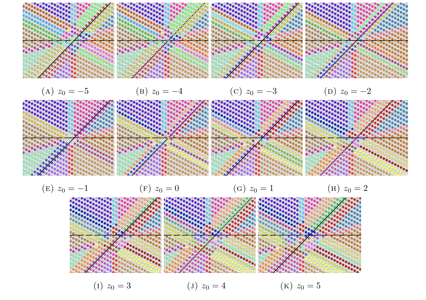
Figure 5. The $\mu=0$ Weyl alternation diagrams for $\mathfrak{sl}_{4}(\mathbb{C})$. The horizontal axis is the real span of $\varpi_{1}$, while the other is the real span of $\varpi_{2}$. The key for these diagram is given in Appendix A.

Another set of diagrams associated to Weyl alternation sets are known as empty regions. We recall that for a fixed $\mu$ in the root lattice, the empty region consists of the set of weights $\lambda$ on the root lattice for which $\mathcal{A}(\lambda,\mu)=\emptyset$. In the following examples, we fix $\mu$ in the root lattice, color red every weight $\lambda$ in the root lattice for which $\mathcal{A}(\lambda,\mu)=0$, and give a geometric description and visualization of the empty region. Note that at times we increase the size of the vertices to better illustrate the behavior of the empty region.

1. : $\mu=n\alpha_{1}$. This empty region is in the shape of a tetrahedron. Additionally, the tetrahedron increases in size as the coefficient of $\alpha_{1}$ increases.

   

2. : $\mu=n\alpha_{2}$. This empty region takes the form of a cube. As before, the cube increases in size as the coefficient of $\alpha_{2}$ increases.

   

3. : $\mu=n\alpha_{3}$. This empty region forms a tetrahedron but with a different orientation than when $\mu=n\alpha_{1}$. As before, the tetrahedron increases in size as the coefficient of $\alpha_{3}$ increases.

   

4. : $\mu=n\alpha_{1}+n\alpha_{2}$. Once again the empty region is a tetrahedron, but we observe that each face shows a set of points near their center. As $n$ increases, so does size of the region.

   

5. : $\mu=n\alpha_{2}+n\alpha_{3}$. The empty region is a tetrahedron with a few points coming out of it. However, the orientation and the size is different from Case 4. As the coefficients for $\alpha_{2},\alpha_{3}$ increase, the shape gets bigger.

   

6. : $\mu=n\alpha_{1}+n\alpha_{3}$. The empty region is a stellated octahedron, being formed by two tetrahedrons. As before, the size of the region grows as $n$ grows.

   

7. : $\mu=n\alpha_{1}+n\alpha_{2}+n\alpha_{3}$. The empty region is a stellated octahedron, being formed by two tetrahedrons. Note that as $n$ grows, so does the size of the region.

   

8. : $\mu=m\alpha_{1}+n\alpha_{2}+k\alpha_{3}$. Here, note that we let $m,n,$ and $k$ be of different parity. When $m,k$ are odd and $n$ is even, the empty region is a tetrahedron. However, if $n$ is odd and $m,k$ are even, we get a stellated octahedron, with one tetrahedron smaller than the other. These shapes seem to be consistently determined by the parity of $m,n,k$ as described. Again, as the coefficients $m,n,k$ grow, so does the size of the region.

   

5. The $q$-analog of Kostant’s weight multiplicity formula

In this section we use Theorem 1 and Theorem 2 to give a formula for the $q$-multiplicity of a weight $\mu$ in $L(\lambda)$, a highest weight irreducible representation of $\mathfrak{sl}_{4}(\mathbb{C})$ with highest weight $\lambda$. We begin by letting $\lambda=m\varpi_{1}+n\varpi_{2}+k\varpi_{3}$ and $\mu=c_{1}\varpi_{1}+c_{2}\varpi_{2}+c_{3}\varpi_{3}$, with $m,n,k,c_{1},c_{2},c_{3}\in\mathbb{N}$, and we set the notation for the rest of the section as given in Table 1.

Theorem 3.

Let $\lambda=m\varpi_{1}+n\varpi_{2}+k\varpi_{3}$ and $\mu=c_{1}\varpi_{1}+c_{2}\varpi_{2}+c_{3}\varpi_{3}$, with $m,n,k,c_{1},c_{2},c_{3}\in\mathbb{N}$. If $x=\frac{3m+2n+k-3c_{1}-2c_{2}-c_{3}}{4}$, $y=\frac{m+2n+k-c_{1}-2c_{2}-c_{3}}{2}$, and $z=\frac{m+2n+3k-c_{1}-2c_{2}-3c_{3}}{4}$, then

$$m_{q}(\lambda,\mu)=\begin{cases}Z_{1}-Z_{11}-Z_{3}+Z_{5}+Z_{10}-Z_{7}&P_{1},Q_{1},R_{1},Q_{6},R_{4},Q_{5},R_{3}\in\mathbb{N}\ \text{and}\ P_{4},P_{3}\notin\mathbb{N}\\ Z_{1}-Z_{6}-Z_{3}+Z_{4}+Z_{8}-Z_{2}&P_{1},Q_{1},R_{1},P_{4},Q_{6},P_{3},Q_{4}\in\mathbb{N}\ \text{and}\ R_{4},R_{3}\notin\mathbb{N}\\ Z_{1}-Z_{6}-Z_{11}-Z_{3}+Z_{8}+Z_{9}&P_{1},Q_{1},R_{1},P_{4},R_{4},Q_{6},Q_{4}\in\mathbb{N}\ \text{and}\ P_{3},Q_{5},R_{3}\notin\mathbb{N}\\ Z_{1}-Z_{6}-Z_{11}-Z_{3}+Z_{9}+Z_{5}&P_{1},Q_{1},R_{1},P_{4},Q_{6},R_{4},Q_{5}\in\mathbb{N}\ \text{and}\ P_{3},Q_{4},R_{3}\notin\mathbb{N}\\ Z_{1}-Z_{6}-Z_{11}-Z_{3}+Z_{9}&P_{1},Q_{1},R_{1},P_{4},Q_{6},R_{4}\in\mathbb{N}\ \text{and}\ P_{3},Q_{4},Q_{5},R_{3}\notin\mathbb{N}\\ Z_{1}-Z_{11}-Z_{3}+Z_{5}&P_{1},Q_{1},R_{1},Q_{6},R_{4},Q_{5}\in\mathbb{N}\ \text{and}\ P_{4},P_{3},R_{3}\notin\mathbb{N}\\ Z_{1}-Z_{6}-Z_{3}+Z_{9}&P_{1},Q_{1},R_{1},P_{4},R_{4}\in\mathbb{N}\ \text{and}\ Q_{6},Q_{4},Q_{5}\notin\mathbb{N}\\ Z_{1}-Z_{6}-Z_{11}+Z_{8}&P_{1},Q_{1},R_{1},P_{4},Q_{6},Q_{4}\in\mathbb{N}\ \text{and}\ R_{4},P_{3},R_{3}\notin\mathbb{N}\\ Z_{1}-Z_{11}-Z_{3}&P_{1},Q_{1},R_{1},Q_{6},R_{4}\in\mathbb{N}\ \text{and}\ P_{4},P_{3},Q_{5},R_{3}\notin\mathbb{N}\\ Z_{1}-Z_{6}-Z_{11}&P_{1},Q_{1},R_{1},P_{4},Q_{6}\in\mathbb{N}\ \text{and}\ R_{4},P_{3},Q_{4},R_{3}\notin\mathbb{N}\\ Z_{1}-Z_{3}&P_{1},Q_{1},R_{1},R_{4}\in\mathbb{N}\ \text{and}\ Q_{6},P_{4},Q_{5}\notin\mathbb{N}\ \text{and}\ (P_{3}\notin\mathbb{N}\ \text{or}\ Q_{4}\notin\mathbb{N})\\ Z_{1}-Z_{11}&P_{1},Q_{1},R_{1},Q_{6}\in\mathbb{N}\ \text{and}\ P_{4},R_{4},R_{3},P_{3}\notin\mathbb{N}\\ Z_{1}-Z_{6}&P_{1},Q_{1},R_{1},P_{4}\in\mathbb{N}\ \text{and}\ Q_{6},R_{4},Q_{4}\notin\mathbb{N}\ \text{and}\ (Q_{5}\notin\mathbb{N}\ \text{or}\ R_{3}\notin\mathbb{N})\\ Z_{1}&P_{1},Q_{1},R_{1}\in\mathbb{N}\ \text{and}\ R_{4},P_{4},Q_{6}\notin\mathbb{N}\ \text{and}\ (P_{3}\notin\mathbb{N}\ \text{or}\ Q_{4}\notin\mathbb{N})\\ &\text{and}\ (Q_{5}\notin\mathbb{N}\ \text{or}\ R_{3}\notin\mathbb{N})\\ 0&\textnormal{otherwise,}\end{cases}$$

where $Z_{1},\dots,Z_{11}$ are defined as in Appendix B.

Proof.

Since $m,n,k,c_{1},c_{2},c_{3}\in\mathbb{N}$, we have $P_{2}$, $Q_{2}$, $R_{2}$ are less than zero by inspection, and a straightforward substitution shows that $Q_{3}=-2m-2k-2c_{1}-4c_{2}-2c_{3}-3<0$. Consequently, $\wp(\sigma(\lambda+\mu)-(\rho+\mu))=0$ for all

$$\sigma\in W_{0}:=\left\{\begin{matrix}s_{2}s_{3}s_{1},s_{3}s_{2}s_{1},s_{2}s_{3}s_{2}s_{1},s_{3}s_{1}s_{2}s_{1},s_{2}s_{3}s_{1}s_{2},s_{2}s_{3}s_{1}s_{2}s_{1},\\ s_{1}s_{2}s_{3},s_{1}s_{2}s_{3}s_{2},s_{1}s_{2}s_{3}s_{1},s_{1}s_{2}s_{3}s_{2}s_{1},s_{1}s_{2}s_{3}s_{1}s_{2},s_{1}s_{2}s_{3}s_{1}s_{2}s_{1}\end{matrix}\right\}.$$

Thus, the only possible Weyl group elements contributing nontrivially to $m_{q}(\lambda,\mu)$ are those in $W\setminus W_{0}$. Table 1 presents our notation for writing $\sigma(\lambda+\rho)-\rho-\mu$ as a nonnegative integral sum of simple roots for all $\sigma\in W$ and in particular for $\sigma\in W\setminus W_{0}$.

Consider the case $\sigma=s_{3}s_{1}s_{2}$. Note that

$$P_{3}=\frac{-m-2n+k-3c_{1}-2c_{2}-c_{3}}{4}-2\qquad\mbox{and}\qquad R_{3}=\frac{m-2n-k-c_{1}-2c_{2}-3c_{3}}{4}-2.$$

In order for us to have $\wp_{q}(s_{3}s_{1}s_{2}(\lambda+\rho)-(\rho+\mu))>0$, we must have in particular that $P_{3}\geq 0$ and $R_{3}\geq 0$. As a result, we have that

$$k \geq 8+m+2n+3c_{1}+2c_{2}+c_{3}\text{ and }k\leq-8+m-2n-c_{1}-2c_{2}-3c_{3}.$$

It then follows that

$$8+m+2n+3c_{1}+2c_{2}+c_{3}\leq-8+m-2n-c_{1}-2c_{2}-3c_{3},$$

which implies $0\geq 16+4n+4c_{1}+4c_{2}+4c_{3}$. Since $n,c_{1},c_{1},c_{3}\geq 0$, this is a contradiction, and thus $\wp_{q}(s_{3}s_{1}s_{2}(\lambda+\rho)-(\rho+\mu))=0$ for all $\lambda,\mu$ in the nonnegative octant of the fundamental weight lattice.

Hence, the only remaining elements of the Weyl group for which it is a possibility that $\wp_{q}(\sigma(\lambda+\rho)-(\rho+\mu))>0$ are those in Table 3.

$\sigma$	$\xi=\sigma(\lambda+\rho)-(\rho+\mu)$	$\wp_{q}(\xi)$
1	$P_{1}\alpha_{1}+Q_{1}\alpha_{2}+R_{1}\alpha_{3}$	$Z_{1}$
$s_{1}s_{2}s_{1}$	$P_{3}\alpha_{1}+Q_{4}\alpha_{2}+R_{1}\alpha_{3}$	$Z_{2}$
$s_{3}$	$P_{1}\alpha_{1}+Q_{1}\alpha_{2}+R_{4}\alpha_{3}$	$Z_{3}$
$s_{1}s_{2}$	$P_{3}\alpha_{1}+Q_{6}\alpha_{2}+R_{1}\alpha_{3}$	$Z_{4}$
$s_{2}s_{3}$	$P_{1}\alpha_{1}+Q_{5}\alpha_{2}+R_{4}\alpha_{3}$	$Z_{5}$
$s_{1}$	$P_{4}\alpha_{1}+Q_{1}\alpha_{2}+R_{1}\alpha_{3}$	$Z_{6}$
$s_{2}s_{3}s_{2}$	$P_{1}\alpha_{1}+Q_{5}\alpha_{2}+R_{3}\alpha_{3}$	$Z_{7}$
$s_{2}s_{1}$	$P_{4}\alpha_{1}+Q_{4}\alpha_{2}+R_{1}\alpha_{3}$	$Z_{8}$
$s_{3}s_{1}$	$P_{4}\alpha_{1}+Q_{1}\alpha_{2}+R_{4}\alpha_{3}$	$Z_{9}$
$s_{3}s_{2}$	$P_{1}\alpha_{1}+Q_{6}\alpha_{2}+R_{3}\alpha_{3}$	$Z_{10}$
$s_{2}$	$P_{1}\alpha_{1}+Q_{6}\alpha_{2}+R_{1}\alpha_{3}$	$Z_{11}$

$P_{1}=x$

$P_{3}=-c_{1}-c_{2}-y+z-2$

$P_{4}=-c_{1}-x+y-1$

$Q_{1}=y$

$Q_{4}=-c_{1}-c_{2}-x+z-2$

$Q_{5}=-c_{2}-c_{3}+x-z-2$

$Q_{6}=-c_{2}+x-y+z-1$

$R_{1}=z$

$R_{3}=-c_{2}-c_{3}+x-y-2$

$R_{4}=-c_{3}+y-z-1$

Table 3. Notation for $\sigma(\lambda+\rho)-\rho-\mu$ when $\sigma\in W\setminus(W_{0}\cup\{s_{3}s_{1}s_{2}\})$.

For each of the elements in Table 3 we have that

$$1\in\mathcal{A}(\lambda,\mu) \Longleftrightarrow P_{1},Q_{1},R_{1}\in\mathbb{N},$$

$$s_{1}\in\mathcal{A}(\lambda,\mu) \Longleftrightarrow P_{4},Q_{1},R_{1}\in\mathbb{N},$$

$$s_{2}\in\mathcal{A}(\lambda,\mu) \Longleftrightarrow P_{1},Q_{6},R_{1}\in\mathbb{N},$$

$$s_{3}\in\mathcal{A}(\lambda,\mu) \Longleftrightarrow P_{1},Q_{1},R_{4}\in\mathbb{N},$$

$$s_{1}s_{2}\in\mathcal{A}(\lambda,\mu) \Longleftrightarrow P_{3},Q_{6},R_{1}\in\mathbb{N},$$

$$s_{2}s_{1}\in\mathcal{A}(\lambda,\mu) \Longleftrightarrow P_{4},Q_{4},R_{1}\in\mathbb{N},$$

$$s_{3}s_{1}\in\mathcal{A}(\lambda,\mu) \Longleftrightarrow P_{4},Q_{1},R_{4}\in\mathbb{N},$$

$$s_{2}s_{3}\in\mathcal{A}(\lambda,\mu) \Longleftrightarrow P_{1},Q_{5},R_{4}\in\mathbb{N},$$

$$s_{3}s_{2}\in\mathcal{A}(\lambda,\mu) \Longleftrightarrow P_{1},Q_{6},R_{3}\in\mathbb{N},$$

$$s_{1}s_{2}s_{1}\in\mathcal{A}(\lambda,\mu) \Longleftrightarrow P_{3},Q_{4},R_{1}\in\mathbb{N},$$

$$s_{2}s_{3}s_{2}\in\mathcal{A}(\lambda,\mu) \Longleftrightarrow P_{1},Q_{5},R_{3}\in\mathbb{N}.$$

Intersecting these inequalities and applying the integrality conditions from Section 4.1, we find that our Weyl alternation set for $\lambda$ and $\mu$ are

$$\mathcal{A}(\lambda,\mu)=\begin{cases}{\{1\}}&R_{1},P_{1},Q_{1}\in\mathbb{N}\text{ and }Q_{6},R_{4},P_{4}\notin\mathbb{N}\text{ and}\\ &(Q_{5}\notin\mathbb{N}\text{ or }R_{3}\notin\mathbb{N})\text{ and }(P_{3}\notin\mathbb{N}\text{ or }Q_{4}\notin\mathbb{N})\\ {\{1,s_{2}\}}&R_{1},Q_{6},P_{1},Q_{1}\in\mathbb{N}\text{ and }P_{3},R_{4},R_{3},P_{4}\notin\mathbb{N}\\ {\{1,s_{3}\}}&R_{1},P_{1},R_{4},Q_{1}\in\mathbb{N}\text{ and }Q_{6},Q_{5},P_{4}\notin\mathbb{N}\text{ and }\\ &(P_{3}\notin\mathbb{N}\text{ or }Q_{4}\notin\mathbb{N})\\ {\{1,s_{1}\}}&R_{1},P_{1},Q_{1},P_{4}\in\mathbb{N}\text{ and }Q_{6},Q_{4},R_{4}\notin\mathbb{N}\text{ and }\\ &(Q_{5}\notin\mathbb{N}\text{ or }R_{3}\notin\mathbb{N})\\ {\{1,s_{3},s_{2}\}}&{R_{1},Q_{6},P_{1},R_{4},Q_{1}\in\mathbb{N}\text{ and }P_{3},Q_{5},R_{3},P_{4}\notin\mathbb{N}}\\ {\{1,s_{2},s_{1}\}}&{R_{1},Q_{6},P_{1},Q_{1},P_{4}\in\mathbb{N}\text{ and }P_{3},Q_{4},R_{4},R_{3}\notin\mathbb{N}}\\ {\{1,s_{3},s_{2}s_{3},s_{2}\}}&{R_{1},Q_{5},Q_{1},R_{4},Q_{6},P_{1}\in\mathbb{N}\text{ and }P_{3},R_{3},P_{4}\notin\mathbb{N}}\\ {\{s_{1},s_{3}s_{1},s_{3},1\}}&{R_{1},P_{1},R_{4},Q_{1},P_{4}\in\mathbb{N}\text{ and }Q_{6},Q_{5},Q_{4}\notin\mathbb{N}}\\ {\{s_{1},s_{2},1,s_{2}s_{1}\}}&{R_{1},Q_{1},P_{4},Q_{6},P_{1},Q_{4}\in\mathbb{N}\text{ and }P_{3},R_{4},R_{3}\notin\mathbb{N}}\\ {\{s_{1},s_{3}s_{1},s_{3},s_{2},1\}}&{R_{1},Q_{1},P_{4},R_{4},Q_{6},P_{1}\in\mathbb{N}\text{ and }P_{3},Q_{5},Q_{4},R_{3}\notin\mathbb{N}}\\ {\{1,s_{3},s_{2}s_{3},s_{2},s_{3}s_{1},s_{1}\}}&{R_{1},Q_{5},Q_{1},P_{4},R_{4},Q_{6},P_{1}\in\mathbb{N}\text{ and }P_{3},Q_{4},R_{3}\notin\mathbb{N}}\\ {\{1,s_{3}s_{1},s_{2}s_{1},s_{3},s_{2},s_{1}\}}&{R_{1},Q_{1},P_{4},R_{4},Q_{6},P_{1},Q_{4}\in\mathbb{N}\text{ and }P_{3},Q_{5},R_{3}\notin\mathbb{N}}\\ {\{1,s_{2}s_{3},s_{3},s_{2},s_{2}s_{3}s_{2},s_{3}s_{2}\}}&{R_{1},Q_{5},Q_{1},R_{3},R_{4},Q_{6},P_{1}\in\mathbb{N}\text{ and }P_{3},P_{4}\notin\mathbb{N}}\\ {\{1,s_{1}s_{2}s_{1},s_{2}s_{1},s_{2},s_{1},s_{1}s_{2}\}}&{R_{1},Q_{1},P_{4},P_{3},Q_{6},P_{1},Q_{4}\in\mathbb{N}\text{ and }R_{4},R_{3}\notin\mathbb{N}}.\\ \end{cases}$$

The result now follows from applying Theorem 1 to evaluate the associated $q$-analog of Kostant’s partition function for each element in the associated Weyl alternation set. In Appendix B to describe concretely each of the polynomials $Z_{1},\ldots,Z_{11}$. ∎

We end this section by applying Theorem 3 to compute a few $q$-weight multiplicities.

Example 3.

Let $\lambda=\alpha_{1}+\alpha_{2}+\alpha_{3}$ and $\mu=0$. Hence $m=1,n=0,k=1$, and $c_{1}=c_{2}=c_{3}=0$, from which we obtain $x=y=z=1$, and, hence, $\lambda=\omega_{1}+\omega_{3}.$ This means that $P_{1}=Q_{1}=R_{1}=1$, $P_{3}=-2$, $P_{4}=-1$, $Q_{5}=-2$, $Q_{6}=-2$, $R_{4}=-1.$ Since, $P_{1},Q_{1},R_{1}\in\mathbb{N}$ and $P_{3},P_{4},Q_{5},Q_{6},R_{4}\notin\mathbb{N},$ then by Theorem 3 we have that

$$m_{q}(\varpi_{1}+\varpi_{3},0) =Z_{1}=\wp_{q}(P_{1}\alpha_{1}+Q_{1}\alpha_{2}+R_{1}\alpha_{3})=\wp_{q}(\alpha_{1}+\alpha_{2}+\alpha_{3}).$$

Applying the formula for $Z_{1}$ in Appendix B we find that $t=2,L=0,1\leq i\leq 3.$ Using our closed formula in Theorem 1, part (1) gives us the final result

$$m_{q}(\varpi_{1}+\varpi_{3},0) =q^{1}+q^{2}+q^{3}.$$

Evaluating at $q=1$ yields $m(\varpi_{1}+\varpi_{3},0)=1+1+1=3$. We recall, that when $\lambda$ is the highest root, $m(\lambda,0)$ is the multiplicity of the zero-weight in the adjoint representation of $\mathfrak{sl}_{4}(\mathbb{C})$. This equals the rank of $\mathfrak{sl}_{4}(\mathbb{C})$ which is indeed 3.

Example 4.

Let $\lambda=\varpi_{1}+2\varpi_{2}+3\varpi_{3}$ and $\mu=\varpi_{1}+\varpi_{2}+\varpi_{3}$. Hence $m=1,n=2,k=3$, and $c_{1}=c_{2}=c_{3}=1$, from which we obtain $x=1,y=2,z=2$, and, hence, $P_{1}=1$, $Q_{1}=2$, $R_{1}=2$, $R_{4}=-2$, $P_{4}=-1$, $Q_{6}=-1$, $P_{3}=-4$, $Q_{5}=-5.$ Since $P_{1},Q_{1},R_{1}\in\mathbb{N}$ and $R_{4},P_{4},Q_{6},P_{3},Q_{5}\notin\mathbb{N}$, then by Theorem 3 we have that

$$m_{q}(\varpi_{1}+2\varpi_{2}+3\varpi_{3},\varpi_{1}+\varpi_{2}+\varpi_{3}) =Z_{1}=\wp_{q}(P_{1}\alpha_{1}+Q_{1}\alpha_{2}+R_{1}\alpha_{3})=\wp_{q}(\alpha_{1}+2\alpha_{2}+2\alpha_{3}).$$

Applying the formula for $Z_{1}$ in Appendix B we find that $t=3$, $F_{1}=1$, $F_{2}=1$, $L=0$, and $J=-1$. Then, since $J<0$, we find that the coefficient of $q^{2}$ is $c_{2}=1$. Applying our closed formula in a similar fashion in the case where $i=2,3,4,5$ gives us the final result

$$m_{q}(\varpi_{1}+2\varpi_{2}+3\varpi_{3},\varpi_{1}+\varpi_{2}+\varpi_{3}) =q^{2}+3q^{3}+2q^{4}+q^{5}.$$

Evaluating at $q=1$ yields $m(\varpi_{1}+2\varpi_{2}+3\varpi_{3},\varpi_{1}+\varpi_{2}+\varpi_{3})=1+3+2+1=7.$

Example 5.

Let $\lambda=\varpi_{1}+3\varpi_{2}$ and $\mu=\varpi_{1}+\varpi_{2}$. Hence, $P_{1}=1$, $Q_{1}=2$, $R_{1}=1$, $R_{4}=0$, $Q_{6}=-2$, $P_{4}=-1$, $Q_{5}=-3$, $P_{3}=-5.$ Note that $P_{1},Q_{1},R_{1},R_{4}\in\mathbb{N}$ and $Q_{6},P_{4},Q_{5},P_{3}\notin\mathbb{N}$. Thus, by Theorem 3, we have that

$$m_{q}(\varpi_{1}+3\varpi_{2},\varpi_{1}+\varpi_{2}) =Z_{1}-Z_{3}=\wp_{q}(\alpha_{1}+2\alpha_{2}+\alpha_{3})-\wp_{q}(\alpha_{1}+2\alpha_{2}).$$

Applying the formula for $Z_{1}$ and $Z_{3}$ in Appendix B we find that $m_{q}(\varpi_{1}+3\varpi_{2},\varpi_{1}+\varpi_{2})=q^{2}+q^{3}+q^{4}.$ Evaluating this polynomial at $q=1$ yields $m(\varpi_{1}+3\varpi_{2},\varpi_{1}+\varpi_{2})=1+1+1=3.$

6. Future Work

As we showed in Section 3, for $i\in\mathbb{N}$ the set of partitions of weights as sums of exactly $i$ positive roots of the Lie algebra $\mathfrak{sl}_{4}(\mathbb{C})$ are in bijection with certain subsets of $\{{\color[rgb]{1,0,0}1_{r}},{\color[rgb]{0,0,1}1_{b}},2\}$-partitions of $i$. We believe that is just one occurrence of such a bijection. Hence we pose the following.

Problem 1.

Characterize sets of restricted colored integer partitions that are in bijection with partitions of weights as sums of a certain number of positive roots of a Lie algebra.

An answer to this question would elucidate and strengthen the initial connection we have made between restricted colored integer partitions and the representation theory of Lie algebras. A connection which was asked about by Corteel and Lovejoy in [4].

Appendix A Theorem 2: Weyl alternation sets of $\mathfrak{sl}_{4}(\mathbb{C})$

Table 4 provides the reduced expression of $\sigma(\lambda+\rho)-\rho-\mu$ after the substitutions for the integrality condition in Lemma 1 are applied.

$\sigma\in W$	$\sigma(\lambda+\rho)-\rho-\mu$
1	$P_{1}\alpha_{1}+Q_{1}\alpha_{2}+R_{1}\alpha_{3}$
$s_{1}$	$P_{4}\alpha_{1}+Q_{1}\alpha_{2}+R_{1}\alpha_{3}$
$s_{2}$	$P_{1}\alpha_{1}+Q_{6}\alpha_{2}+R_{1}\alpha_{3}$
$s_{3}$	$P_{1}\alpha_{1}+Q_{1}\alpha_{2}+R_{4}\alpha_{3}$
$s_{1}s_{2}$	$P_{3}\alpha_{1}+Q_{6}\alpha_{2}+R_{1}\alpha_{3}$
$s_{2}s_{1}$	$P_{4}\alpha_{1}+Q_{4}\alpha_{2}+R_{1}\alpha_{3}$
$s_{2}s_{3}$	$P_{1}\alpha_{1}+Q_{5}\alpha_{2}+R_{4}\alpha_{3}$
$s_{3}s_{1}$	$P_{4}\alpha_{1}+Q_{1}\alpha_{2}+R_{4}\alpha_{3}$
$s_{3}s_{2}$	$P_{1}\alpha_{1}+Q_{6}\alpha_{2}+R_{3}\alpha_{3}$
$s_{1}s_{2}s_{1}$	$P_{3}\alpha_{1}+Q_{4}\alpha_{2}+R_{1}\alpha_{3}$
$s_{1}s_{2}s_{3}$	$P_{2}\alpha_{1}+Q_{5}\alpha_{2}+R_{4}\alpha_{3}$
$s_{2}s_{3}s_{1}$	$P_{4}\alpha_{1}+Q_{3}\alpha_{2}+R_{4}\alpha_{3}$
$s_{2}s_{3}s_{2}$	$P_{1}\alpha_{1}+Q_{5}\alpha_{2}+R_{3}\alpha_{3}$
$s_{3}s_{1}s_{2}$	$P_{3}\alpha_{1}+Q_{6}\alpha_{2}+R_{3}\alpha_{3}$
$s_{3}s_{2}s_{1}$	$P_{4}\alpha_{1}+Q_{4}\alpha_{2}+R_{2}\alpha_{3}$
$s_{1}s_{2}s_{3}s_{1}$	$P_{2}\alpha_{1}+Q_{3}\alpha_{2}+R_{4}\alpha_{3}$
$s_{1}s_{2}s_{3}s_{2}$	$P_{2}\alpha_{1}+Q_{5}\alpha_{2}+R_{3}\alpha_{3}$
$s_{2}s_{3}s_{1}s_{2}$	$P_{3}\alpha_{1}+Q_{2}\alpha_{2}+R_{3}\alpha_{3}$
$s_{2}s_{3}s_{2}s_{1}$	$P_{4}\alpha_{1}+Q_{3}\alpha_{2}+R_{2}\alpha_{3}$
$s_{3}s_{1}s_{2}s_{1}$	$P_{3}\alpha_{1}+Q_{4}\alpha_{2}+R_{2}\alpha_{3}$
$s_{1}s_{2}s_{3}s_{1}s_{2}$	$P_{2}\alpha_{1}+Q_{2}\alpha_{2}+R_{3}\alpha_{3}$
$s_{1}s_{2}s_{3}s_{2}s_{1}$	$P_{2}\alpha_{1}+Q_{3}\alpha_{2}+R_{2}\alpha_{3}$
$s_{2}s_{3}s_{1}s_{2}s_{1}$	$P_{3}\alpha_{1}+Q_{2}\alpha_{2}+R_{2}\alpha_{3}$
$s_{1}s_{2}s_{3}s_{1}s_{2}s_{1}$	$P_{2}\alpha_{1}+Q_{2}\alpha_{2}+R_{2}\alpha_{3}$

$P_{1}=x$

$P_{2}=-c_{1}-c_{2}-c_{3}-z-3$

$P_{3}=-c_{1}-c_{2}-y+z-2$

$P_{4}=-c_{1}-x+y-1$

$Q_{1}=y$

$Q_{2}=-c_{1}-2c_{2}-c_{3}-y-4$

$Q_{3}=-c_{1}-c_{2}-c_{3}-x+y-z-3$

$Q_{4}=-c_{1}-c_{2}-x+z-2$

$Q_{5}=-c_{2}-c_{3}+x-z-2$

$Q_{6}=-c_{2}+x-y+z-1$

$R_{1}=z$

$R_{2}=-c_{1}-c_{2}-c_{3}-x-3$

$R_{3}=-c_{2}-c_{3}+x-y-2$

$R_{4}=-c_{3}+y-z-1$

Table 4. Notation for $\sigma(\lambda+\rho)-\rho-\mu$ as a sum of simple roots for each $\sigma\in W$.

Thus, the conditions Table 5 describe explicitly when a given element $\sigma\in W$ is in $\mathcal{A}(\lambda,\mu)$.

$K_{1}:$	$P_{1}=x\in\mathbb{N}$
$K_{2}:$	$P_{2}-c_{1}-c_{2}-c_{3}-z-3\in\mathbb{N}$
$K_{3}:$	$P_{3}=-c_{1}-c_{2}-y+z-2\in\mathbb{N}$
$K_{4}:$	$P_{4}=-c_{1}-x+y-1\in\mathbb{N}$
$K_{5}:$	$Q_{1}=y\in\mathbb{N}$
$K_{6}:$	$Q_{2}=-c_{1}-2c_{2}-c_{3}-y-4\in\mathbb{N}$
$K_{7}:$	$Q_{3}=-c_{1}-c_{2}-c_{3}-x+y-z-3\in\mathbb{N}$
$K_{8}:$	$Q_{4}=-c_{1}-c_{2}-x+z-2\in\mathbb{N}$
$K_{9}:$	$Q_{5}=-c_{2}-c_{3}+x-z-2\in\mathbb{N}$
$K_{10}:$	$Q_{6}=-c_{2}+x-y+z-1\in\mathbb{N}$
$K_{11}:$	$R_{1}=z\in\mathbb{N}$
$K_{12}:$	$R_{2}=-c_{1}-c_{2}-c_{3}-x-3\in\mathbb{N}$
$K_{13}:$	$R_{3}=-c_{2}-c_{3}+x-y-2\in\mathbb{N}$
$K_{14}:$	$R_{4}=-c_{3}+y-z-1\in\mathbb{N}$

Table 5. Conditions used in defining the Weyl alternation sets of $\mathfrak{sl}_{4}(\mathbb{C})$.

Using the conditions as listed in Table 5, and letting $\neg$ denote negation and $\vee$ denote or, then the Weyl alternation sets are as follows:

1. $\mathcal{A}(\lambda,\mu)=\{1\}$ if $K_{11}$, $K_{1}$, $K_{5}$,$\neg K_{10}$, $\neg K_{4}$, $\neg K_{14}$, $\neg K_{2}$ $\vee$ $\neg K_{7}$ $\vee$ $\neg K_{12}$, $\neg K_{2}$ $\vee$ $\neg K_{6}$ $\vee$ $\neg K_{12}$, $\neg K_{3}$ $\vee$ $\neg K_{6}$ $\vee$ $\neg K_{12}$, $\neg K_{3}$ $\vee$ $\neg K_{8}$, $\neg K_{9}$ $\vee$ $\neg K_{13}$, $\neg K_{2}$ $\vee$ $\neg K_{6}$ $\vee$ $\neg K_{13}$, $\neg K_{3}$ $\vee$ $\neg K_{6}$ $\vee$ $\neg K_{13}$,

2. $\mathcal{A}(\lambda,\mu)=\{s_{1}\}$ if $K_{11}$, $K_{5}$, $K_{4}$,$\neg K_{1}$, $\neg K_{14}$, $\neg K_{8}$, $\neg K_{2}$ $\vee$ $\neg K_{6}$ $\vee$ $\neg K_{12}$, $\neg K_{3}$ $\vee$ $\neg K_{6}$ $\vee$ $\neg K_{12}$, $\neg K_{3}$ $\vee$ $\neg K_{10}$, $\neg K_{12}$ $\vee$ $\neg K_{7}$, $\neg K_{2}$ $\vee$ $\neg K_{6}$ $\vee$ $\neg K_{13}$, $\neg K_{3}$ $\vee$ $\neg K_{6}$ $\vee$ $\neg K_{13}$, $\neg K_{2}$ $\vee$ $\neg K_{9}$ $\vee$ $\neg K_{13}$,

3. $\mathcal{A}(\lambda,\mu)=\{s_{2}\}$ if $K_{11}$, $K_{10}$, $K_{1}$,$\neg K_{5}$, $\neg K_{13}$, $\neg K_{3}$, $\neg K_{2}$ $\vee$ $\neg K_{7}$ $\vee$ $\neg K_{12}$, $\neg K_{2}$ $\vee$ $\neg K_{6}$ $\vee$ $\neg K_{12}$, $\neg K_{2}$ $\vee$ $\neg K_{7}$ $\vee$ $\neg K_{14}$, $\neg K_{9}$ $\vee$ $\neg K_{14}$, $\neg K_{12}$ $\vee$ $\neg K_{7}$ $\vee$ $\neg K_{4}$, $\neg K_{7}$ $\vee$ $\neg K_{14}$ $\vee$ $\neg K_{4}$, $\neg K_{8}$ $\vee$ $\neg K_{4}$,

4. $\mathcal{A}(\lambda,\mu)=\{s_{3}\}$ if $K_{1}$, $K_{14}$, $K_{5}$,$\neg K_{11}$, $\neg K_{9}$, $\neg K_{4}$, $\neg K_{2}$ $\vee$ $\neg K_{6}$ $\vee$ $\neg K_{12}$, $\neg K_{2}$ $\vee$ $\neg K_{7}$, $\neg K_{10}$ $\vee$ $\neg K_{13}$, $\neg K_{3}$ $\vee$ $\neg K_{6}$ $\vee$ $\neg K_{12}$, $\neg K_{3}$ $\vee$ $\neg K_{8}$ $\vee$ $\neg K_{12}$, $\neg K_{2}$ $\vee$ $\neg K_{6}$ $\vee$ $\neg K_{13}$, $\neg K_{3}$ $\vee$ $\neg K_{6}$ $\vee$ $\neg K_{13}$,

5. $\mathcal{A}(\lambda,\mu)=\{s_{1}s_{2}\}$ if $K_{3}$, $K_{10}$, $K_{11}$,$\neg K_{1}$, $\neg K_{8}$, $\neg K_{13}$, $\neg K_{2}$ $\vee$ $\neg K_{7}$ $\vee$ $\neg K_{12}$, $\neg K_{2}$ $\vee$ $\neg K_{7}$ $\vee$ $\neg K_{14}$, $\neg K_{5}$ $\vee$ $\neg K_{4}$, $\neg K_{6}$ $\vee$ $\neg K_{12}$, $\neg K_{2}$ $\vee$ $\neg K_{9}$ $\vee$ $\neg K_{14}$, $\neg K_{12}$ $\vee$ $\neg K_{7}$ $\vee$ $\neg K_{4}$, $\neg K_{7}$ $\vee$ $\neg K_{14}$ $\vee$ $\neg K_{4}$,

6. $\mathcal{A}(\lambda,\mu)=\{s_{2}s_{1}\}$ if $K_{11}$, $K_{8}$, $K_{4}$,$\neg K_{5}$, $\neg K_{3}$, $\neg K_{12}$, $\neg K_{10}$ $\vee$ $\neg K_{1}$, $\neg K_{1}$ $\vee$ $\neg K_{9}$ $\vee$ $\neg K_{14}$, $\neg K_{2}$ $\vee$ $\neg K_{9}$ $\vee$ $\neg K_{14}$, $\neg K_{1}$ $\vee$ $\neg K_{9}$ $\vee$ $\neg K_{13}$, $\neg K_{2}$ $\vee$ $\neg K_{6}$ $\vee$ $\neg K_{13}$, $\neg K_{7}$ $\vee$ $\neg K_{14}$, $\neg K_{2}$ $\vee$ $\neg K_{9}$ $\vee$ $\neg K_{13}$,

7. $\mathcal{A}(\lambda,\mu)=\{s_{2}s_{3}\}$ if $K_{1}$, $K_{9}$, $K_{14}$,$\neg K_{5}$, $\neg K_{2}$, $\neg K_{13}$, $\neg K_{11}$ $\vee$ $\neg K_{10}$, $\neg K_{3}$ $\vee$ $\neg K_{6}$ $\vee$ $\neg K_{12}$, $\neg K_{3}$ $\vee$ $\neg K_{11}$ $\vee$ $\neg K_{8}$, $\neg K_{8}$ $\vee$ $\neg K_{12}$ $\vee$ $\neg K_{4}$, $\neg K_{3}$ $\vee$ $\neg K_{8}$ $\vee$ $\neg K_{12}$, $\neg K_{7}$ $\vee$ $\neg K_{4}$, $\neg K_{11}$ $\vee$ $\neg K_{8}$ $\vee$ $\neg K_{4}$,

8. $\mathcal{A}(\lambda,\mu)=\{s_{3}s_{1}\}$ if $K_{14}$, $K_{5}$, $K_{4}$,$\neg K_{11}$, $\neg K_{1}$, $\neg K_{7}$, $\neg K_{2}$ $\vee$ $\neg K_{6}$ $\vee$ $\neg K_{12}$, $\neg K_{3}$ $\vee$ $\neg K_{6}$ $\vee$ $\neg K_{12}$, $\neg K_{8}$ $\vee$ $\neg K_{12}$, $\neg K_{2}$ $\vee$ $\neg K_{9}$, $\neg K_{2}$ $\vee$ $\neg K_{6}$ $\vee$ $\neg K_{13}$, $\neg K_{3}$ $\vee$ $\neg K_{10}$ $\vee$ $\neg K_{13}$, $\neg K_{3}$ $\vee$ $\neg K_{6}$ $\vee$ $\neg K_{13}$,

9. $\mathcal{A}(\lambda,\mu)=\{s_{3}s_{2}\}$ if $K_{10}$, $K_{1}$, $K_{13}$,$\neg K_{11}$, $\neg K_{9}$, $\neg K_{3}$, $\neg K_{2}$ $\vee$ $\neg K_{7}$ $\vee$ $\neg K_{12}$, $\neg K_{2}$ $\vee$ $\neg K_{7}$ $\vee$ $\neg K_{14}$, $\neg K_{8}$ $\vee$ $\neg K_{12}$ $\vee$ $\neg K_{4}$, $\neg K_{14}$ $\vee$ $\neg K_{5}$, $\neg K_{12}$ $\vee$ $\neg K_{7}$ $\vee$ $\neg K_{4}$, $\neg K_{2}$ $\vee$ $\neg K_{6}$, $\neg K_{7}$ $\vee$ $\neg K_{14}$ $\vee$ $\neg K_{4}$,

10. $\mathcal{A}(\lambda,\mu)=\{s_{1}s_{2}s_{1}\}$ if $K_{3}$, $K_{11}$, $K_{8}$,$\neg K_{10}$, $\neg K_{12}$, $\neg K_{4}$, $\neg K_{1}$ $\vee$ $\neg K_{5}$, $\neg K_{2}$ $\vee$ $\neg K_{7}$ $\vee$ $\neg K_{14}$, $\neg K_{1}$ $\vee$ $\neg K_{9}$ $\vee$ $\neg K_{14}$, $\neg K_{2}$ $\vee$ $\neg K_{9}$ $\vee$ $\neg K_{14}$, $\neg K_{1}$ $\vee$ $\neg K_{9}$ $\vee$ $\neg K_{13}$, $\neg K_{6}$ $\vee$ $\neg K_{13}$, $\neg K_{2}$ $\vee$ $\neg K_{9}$ $\vee$ $\neg K_{13}$,

11. $\mathcal{A}(\lambda,\mu)=\{s_{1}s_{2}s_{3}\}$ if $K_{2}$, $K_{9}$, $K_{14}$,$\neg K_{7}$, $\neg K_{1}$, $\neg K_{13}$, $\neg K_{6}$ $\vee$ $\neg K_{12}$, $\neg K_{3}$ $\vee$ $\neg K_{11}$ $\vee$ $\neg K_{8}$, $\neg K_{8}$ $\vee$ $\neg K_{12}$ $\vee$ $\neg K_{4}$, $\neg K_{3}$ $\vee$ $\neg K_{10}$ $\vee$ $\neg K_{11}$, $\neg K_{3}$ $\vee$ $\neg K_{8}$ $\vee$ $\neg K_{12}$, $\neg K_{5}$ $\vee$ $\neg K_{4}$, $\neg K_{11}$ $\vee$ $\neg K_{8}$ $\vee$ $\neg K_{4}$,

12. $\mathcal{A}(\lambda,\mu)=\{s_{2}s_{3}s_{1}\}$ if $K_{7}$, $K_{14}$, $K_{4}$,$\neg K_{2}$, $\neg K_{12}$, $\neg K_{5}$, $\neg K_{11}$ $\vee$ $\neg K_{10}$ $\vee$ $\neg K_{1}$, $\neg K_{10}$ $\vee$ $\neg K_{1}$ $\vee$ $\neg K_{13}$, $\neg K_{1}$ $\vee$ $\neg K_{9}$, $\neg K_{3}$ $\vee$ $\neg K_{10}$ $\vee$ $\neg K_{11}$, $\neg K_{3}$ $\vee$ $\neg K_{10}$ $\vee$ $\neg K_{13}$, $\neg K_{3}$ $\vee$ $\neg K_{6}$ $\vee$ $\neg K_{13}$, $\neg K_{11}$ $\vee$ $\neg K_{8}$,

13. $\mathcal{A}(\lambda,\mu)=\{s_{2}s_{3}s_{2}\}$ if $K_{1}$, $K_{9}$, $K_{13}$,$\neg K_{10}$, $\neg K_{14}$, $\neg K_{2}$, $\neg K_{11}$ $\vee$ $\neg K_{5}$, $\neg K_{3}$ $\vee$ $\neg K_{11}$ $\vee$ $\neg K_{8}$, $\neg K_{8}$ $\vee$ $\neg K_{12}$ $\vee$ $\neg K_{4}$, $\neg K_{12}$ $\vee$ $\neg K_{7}$ $\vee$ $\neg K_{4}$, $\neg K_{3}$ $\vee$ $\neg K_{8}$ $\vee$ $\neg K_{12}$, $\neg K_{3}$ $\vee$ $\neg K_{6}$, $\neg K_{11}$ $\vee$ $\neg K_{8}$ $\vee$ $\neg K_{4}$,

14. $\mathcal{A}(\lambda,\mu)=\{s_{3}s_{1}s_{2}\}$ if $K_{3}$, $K_{10}$, $K_{13}$,$\neg K_{1}$, $\neg K_{11}$, $\neg K_{6}$, $\neg K_{2}$ $\vee$ $\neg K_{7}$ $\vee$ $\neg K_{12}$, $\neg K_{2}$ $\vee$ $\neg K_{7}$ $\vee$ $\neg K_{14}$, $\neg K_{12}$ $\vee$ $\neg K_{7}$ $\vee$ $\neg K_{4}$, $\neg K_{8}$ $\vee$ $\neg K_{12}$, $\neg K_{14}$ $\vee$ $\neg K_{5}$ $\vee$ $\neg K_{4}$, $\neg K_{7}$ $\vee$ $\neg K_{14}$ $\vee$ $\neg K_{4}$, $\neg K_{2}$ $\vee$ $\neg K_{9}$,

15. $\mathcal{A}(\lambda,\mu)=\{s_{3}s_{2}s_{1}\}$ if $K_{8}$, $K_{4}$, $K_{12}$,$\neg K_{7}$, $\neg K_{3}$, $\neg K_{11}$, $\neg K_{2}$ $\vee$ $\neg K_{6}$, $\neg K_{10}$ $\vee$ $\neg K_{1}$ $\vee$ $\neg K_{13}$, $\neg K_{1}$ $\vee$ $\neg K_{9}$ $\vee$ $\neg K_{14}$, $\neg K_{2}$ $\vee$ $\neg K_{9}$ $\vee$ $\neg K_{14}$, $\neg K_{1}$ $\vee$ $\neg K_{9}$ $\vee$ $\neg K_{13}$, $\neg K_{14}$ $\vee$ $\neg K_{5}$, $\neg K_{2}$ $\vee$ $\neg K_{9}$ $\vee$ $\neg K_{13}$,

16. $\mathcal{A}(\lambda,\mu)=\{s_{1}s_{2}s_{3}s_{1}\}$ if $K_{2}$, $K_{7}$, $K_{14}$,$\neg K_{12}$, $\neg K_{9}$, $\neg K_{4}$, $\neg K_{11}$ $\vee$ $\neg K_{10}$ $\vee$ $\neg K_{1}$, $\neg K_{10}$ $\vee$ $\neg K_{1}$ $\vee$ $\neg K_{13}$, $\neg K_{3}$ $\vee$ $\neg K_{11}$ $\vee$ $\neg K_{8}$, $\neg K_{1}$ $\vee$ $\neg K_{5}$, $\neg K_{3}$ $\vee$ $\neg K_{10}$ $\vee$ $\neg K_{11}$, $\neg K_{6}$ $\vee$ $\neg K_{13}$, $\neg K_{3}$ $\vee$ $\neg K_{10}$ $\vee$ $\neg K_{13}$,

17. $\mathcal{A}(\lambda,\mu)=\{s_{1}s_{2}s_{3}s_{2}\}$ if $K_{2}$, $K_{9}$, $K_{13}$,$\neg K_{14}$, $\neg K_{1}$, $\neg K_{6}$, $\neg K_{7}$ $\vee$ $\neg K_{12}$, $\neg K_{11}$ $\vee$ $\neg K_{5}$ $\vee$ $\neg K_{4}$, $\neg K_{3}$ $\vee$ $\neg K_{11}$ $\vee$ $\neg K_{8}$, $\neg K_{8}$ $\vee$ $\neg K_{12}$ $\vee$ $\neg K_{4}$, $\neg K_{3}$ $\vee$ $\neg K_{8}$ $\vee$ $\neg K_{12}$, $\neg K_{3}$ $\vee$ $\neg K_{10}$, $\neg K_{11}$ $\vee$ $\neg K_{8}$ $\vee$ $\neg K_{4}$,

18. $\mathcal{A}(\lambda,\mu)=\{s_{2}s_{3}s_{1}s_{2}\}$ if $K_{3}$, $K_{6}$, $K_{13}$,$\neg K_{12}$, $\neg K_{2}$, $\neg K_{10}$, $\neg K_{11}$ $\vee$ $\neg K_{1}$ $\vee$ $\neg K_{5}$, $\neg K_{11}$ $\vee$ $\neg K_{5}$ $\vee$ $\neg K_{4}$, $\neg K_{11}$ $\vee$ $\neg K_{8}$, $\neg K_{1}$ $\vee$ $\neg K_{14}$ $\vee$ $\neg K_{5}$, $\neg K_{1}$ $\vee$ $\neg K_{9}$, $\neg K_{14}$ $\vee$ $\neg K_{5}$ $\vee$ $\neg K_{4}$, $\neg K_{7}$ $\vee$ $\neg K_{14}$ $\vee$ $\neg K_{4}$,

19. $\mathcal{A}(\lambda,\mu)=\{s_{2}s_{3}s_{2}s_{1}\}$ if $K_{4}$, $K_{7}$, $K_{12}$,$\neg K_{2}$, $\neg K_{8}$, $\neg K_{14}$, $\neg K_{11}$ $\vee$ $\neg K_{10}$ $\vee$ $\neg K_{1}$, $\neg K_{11}$ $\vee$ $\neg K_{5}$, $\neg K_{10}$ $\vee$ $\neg K_{1}$ $\vee$ $\neg K_{13}$, $\neg K_{3}$ $\vee$ $\neg K_{6}$, $\neg K_{1}$ $\vee$ $\neg K_{9}$ $\vee$ $\neg K_{13}$, $\neg K_{3}$ $\vee$ $\neg K_{10}$ $\vee$ $\neg K_{11}$, $\neg K_{3}$ $\vee$ $\neg K_{10}$ $\vee$ $\neg K_{13}$,

20. $\mathcal{A}(\lambda,\mu)=\{s_{3}s_{1}s_{2}s_{1}\}$ if $K_{3}$, $K_{8}$, $K_{12}$,$\neg K_{6}$, $\neg K_{11}$, $\neg K_{4}$, $\neg K_{2}$ $\vee$ $\neg K_{7}$, $\neg K_{1}$ $\vee$ $\neg K_{9}$ $\vee$ $\neg K_{14}$, $\neg K_{1}$ $\vee$ $\neg K_{14}$ $\vee$ $\neg K_{5}$, $\neg K_{2}$ $\vee$ $\neg K_{9}$ $\vee$ $\neg K_{14}$, $\neg K_{1}$ $\vee$ $\neg K_{9}$ $\vee$ $\neg K_{13}$, $\neg K_{10}$ $\vee$ $\neg K_{13}$, $\neg K_{2}$ $\vee$ $\neg K_{9}$ $\vee$ $\neg K_{13}$,

21. $\mathcal{A}(\lambda,\mu)=\{s_{1}s_{2}s_{3}s_{1}s_{2}\}$ if $K_{2}$, $K_{6}$, $K_{13}$,$\neg K_{12}$, $\neg K_{3}$, $\neg K_{9}$, $\neg K_{11}$ $\vee$ $\neg K_{1}$ $\vee$ $\neg K_{5}$, $\neg K_{7}$ $\vee$ $\neg K_{14}$, $\neg K_{11}$ $\vee$ $\neg K_{5}$ $\vee$ $\neg K_{4}$, $\neg K_{10}$ $\vee$ $\neg K_{1}$, $\neg K_{1}$ $\vee$ $\neg K_{14}$ $\vee$ $\neg K_{5}$, $\neg K_{14}$ $\vee$ $\neg K_{5}$ $\vee$ $\neg K_{4}$, $\neg K_{11}$ $\vee$ $\neg K_{8}$ $\vee$ $\neg K_{4}$,

22. $\mathcal{A}(\lambda,\mu)=\{s_{1}s_{2}s_{3}s_{2}s_{1}\}$ if $K_{2}$, $K_{7}$, $K_{12}$,$\neg K_{6}$, $\neg K_{14}$, $\neg K_{4}$, $\neg K_{11}$ $\vee$ $\neg K_{1}$ $\vee$ $\neg K_{5}$, $\neg K_{11}$ $\vee$ $\neg K_{10}$ $\vee$ $\neg K_{1}$, $\neg K_{10}$ $\vee$ $\neg K_{1}$ $\vee$ $\neg K_{13}$, $\neg K_{3}$ $\vee$ $\neg K_{10}$ $\vee$ $\neg K_{11}$, $\neg K_{3}$ $\vee$ $\neg K_{8}$, $\neg K_{3}$ $\vee$ $\neg K_{10}$ $\vee$ $\neg K_{13}$, $\neg K_{9}$ $\vee$ $\neg K_{13}$,

23. $\mathcal{A}(\lambda,\mu)=\{s_{2}s_{3}s_{1}s_{2}s_{1}\}$ if $K_{3}$, $K_{6}$, $K_{12}$,$\neg K_{2}$, $\neg K_{8}$, $\neg K_{13}$, $\neg K_{11}$ $\vee$ $\neg K_{1}$ $\vee$ $\neg K_{5}$, $\neg K_{11}$ $\vee$ $\neg K_{5}$ $\vee$ $\neg K_{4}$, $\neg K_{1}$ $\vee$ $\neg K_{9}$ $\vee$ $\neg K_{14}$, $\neg K_{1}$ $\vee$ $\neg K_{14}$ $\vee$ $\neg K_{5}$, $\neg K_{10}$ $\vee$ $\neg K_{11}$, $\neg K_{7}$ $\vee$ $\neg K_{4}$, $\neg K_{14}$ $\vee$ $\neg K_{5}$ $\vee$ $\neg K_{4}$,

24. $\mathcal{A}(\lambda,\mu)=\{s_{1}s_{2}s_{3}s_{1}s_{2}s_{1}\}$ if $K_{2}$, $K_{6}$, $K_{12}$,$\neg K_{7}$, $\neg K_{3}$, $\neg K_{13}$, $\neg K_{11}$ $\vee$ $\neg K_{1}$ $\vee$ $\neg K_{5}$, $\neg K_{11}$ $\vee$ $\neg K_{10}$ $\vee$ $\neg K_{1}$, $\neg K_{11}$ $\vee$ $\neg K_{5}$ $\vee$ $\neg K_{4}$, $\neg K_{8}$ $\vee$ $\neg K_{4}$, $\neg K_{1}$ $\vee$ $\neg K_{14}$ $\vee$ $\neg K_{5}$, $\neg K_{9}$ $\vee$ $\neg K_{14}$, $\neg K_{14}$ $\vee$ $\neg K_{5}$ $\vee$ $\neg K_{4}$,

25. $\mathcal{A}(\lambda,\mu)=\{1,s_{1}\}$ if $K_{11}$, $K_{1}$, $K_{5}$, $K_{4}$,$\neg K_{10}$, $\neg K_{14}$, $\neg K_{8}$, $\neg K_{2}$ $\vee$ $\neg K_{6}$ $\vee$ $\neg K_{12}$, $\neg K_{3}$ $\vee$ $\neg K_{6}$ $\vee$ $\neg K_{12}$, $\neg K_{9}$ $\vee$ $\neg K_{13}$, $\neg K_{12}$ $\vee$ $\neg K_{7}$, $\neg K_{2}$ $\vee$ $\neg K_{6}$ $\vee$ $\neg K_{13}$, $\neg K_{3}$ $\vee$ $\neg K_{6}$ $\vee$ $\neg K_{13}$,

26. $\mathcal{A}(\lambda,\mu)=\{1,s_{2}\}$ if $K_{11}$, $K_{10}$, $K_{1}$, $K_{5}$,$\neg K_{4}$, $\neg K_{13}$, $\neg K_{14}$, $\neg K_{3}$, $\neg K_{2}$ $\vee$ $\neg K_{7}$ $\vee$ $\neg K_{12}$, $\neg K_{2}$ $\vee$ $\neg K_{6}$ $\vee$ $\neg K_{12}$,

27. $\mathcal{A}(\lambda,\mu)=\{1,s_{3}\}$ if $K_{11}$, $K_{1}$, $K_{14}$, $K_{5}$,$\neg K_{10}$, $\neg K_{4}$, $\neg K_{9}$, $\neg K_{2}$ $\vee$ $\neg K_{6}$ $\vee$ $\neg K_{12}$, $\neg K_{2}$ $\vee$ $\neg K_{7}$, $\neg K_{3}$ $\vee$ $\neg K_{6}$ $\vee$ $\neg K_{12}$, $\neg K_{3}$ $\vee$ $\neg K_{8}$, $\neg K_{2}$ $\vee$ $\neg K_{6}$ $\vee$ $\neg K_{13}$, $\neg K_{3}$ $\vee$ $\neg K_{6}$ $\vee$ $\neg K_{13}$,

28. $\mathcal{A}(\lambda,\mu)=\{s_{1},s_{2}s_{1}\}$ if $K_{11}$, $K_{8}$, $K_{5}$, $K_{4}$,$\neg K_{1}$, $\neg K_{3}$, $\neg K_{12}$, $\neg K_{14}$, $\neg K_{2}$ $\vee$ $\neg K_{6}$ $\vee$ $\neg K_{13}$, $\neg K_{2}$ $\vee$ $\neg K_{9}$ $\vee$ $\neg K_{13}$,

29. $\mathcal{A}(\lambda,\mu)=\{s_{1},s_{3}s_{1}\}$ if $K_{11}$, $K_{14}$, $K_{5}$, $K_{4}$,$\neg K_{1}$, $\neg K_{7}$, $\neg K_{8}$, $\neg K_{2}$ $\vee$ $\neg K_{6}$ $\vee$ $\neg K_{12}$, $\neg K_{3}$ $\vee$ $\neg K_{6}$ $\vee$ $\neg K_{12}$, $\neg K_{2}$ $\vee$ $\neg K_{9}$, $\neg K_{3}$ $\vee$ $\neg K_{10}$, $\neg K_{2}$ $\vee$ $\neg K_{6}$ $\vee$ $\neg K_{13}$, $\neg K_{3}$ $\vee$ $\neg K_{6}$ $\vee$ $\neg K_{13}$,

30. $\mathcal{A}(\lambda,\mu)=\{s_{2},s_{1}s_{2}\}$ if $K_{11}$, $K_{10}$, $K_{1}$, $K_{3}$,$\neg K_{5}$, $\neg K_{13}$, $\neg K_{8}$, $\neg K_{2}$ $\vee$ $\neg K_{7}$ $\vee$ $\neg K_{12}$, $\neg K_{2}$ $\vee$ $\neg K_{7}$ $\vee$ $\neg K_{14}$, $\neg K_{6}$ $\vee$ $\neg K_{12}$, $\neg K_{9}$ $\vee$ $\neg K_{14}$, $\neg K_{12}$ $\vee$ $\neg K_{7}$ $\vee$ $\neg K_{4}$, $\neg K_{7}$ $\vee$ $\neg K_{14}$ $\vee$ $\neg K_{4}$,

31. $\mathcal{A}(\lambda,\mu)=\{s_{2},s_{3}s_{2}\}$ if $K_{11}$, $K_{10}$, $K_{1}$, $K_{13}$,$\neg K_{5}$, $\neg K_{9}$, $\neg K_{3}$, $\neg K_{2}$ $\vee$ $\neg K_{7}$ $\vee$ $\neg K_{12}$, $\neg K_{2}$ $\vee$ $\neg K_{7}$ $\vee$ $\neg K_{14}$, $\neg K_{12}$ $\vee$ $\neg K_{7}$ $\vee$ $\neg K_{4}$, $\neg K_{2}$ $\vee$ $\neg K_{6}$, $\neg K_{7}$ $\vee$ $\neg K_{14}$ $\vee$ $\neg K_{4}$, $\neg K_{8}$ $\vee$ $\neg K_{4}$,

32. $\mathcal{A}(\lambda,\mu)=\{s_{3},s_{2}s_{3}\}$ if $K_{1}$, $K_{9}$, $K_{5}$, $K_{14}$,$\neg K_{11}$, $\neg K_{2}$, $\neg K_{13}$, $\neg K_{4}$, $\neg K_{3}$ $\vee$ $\neg K_{6}$ $\vee$ $\neg K_{12}$, $\neg K_{3}$ $\vee$ $\neg K_{8}$ $\vee$ $\neg K_{12}$,

33. $\mathcal{A}(\lambda,\mu)=\{s_{3},s_{3}s_{1}\}$ if $K_{1}$, $K_{14}$, $K_{5}$, $K_{4}$,$\neg K_{11}$, $\neg K_{9}$, $\neg K_{7}$, $\neg K_{2}$ $\vee$ $\neg K_{6}$ $\vee$ $\neg K_{12}$, $\neg K_{10}$ $\vee$ $\neg K_{13}$, $\neg K_{3}$ $\vee$ $\neg K_{6}$ $\vee$ $\neg K_{12}$, $\neg K_{8}$ $\vee$ $\neg K_{12}$, $\neg K_{2}$ $\vee$ $\neg K_{6}$ $\vee$ $\neg K_{13}$, $\neg K_{3}$ $\vee$ $\neg K_{6}$ $\vee$ $\neg K_{13}$,

34. $\mathcal{A}(\lambda,\mu)=\{s_{1}s_{2},s_{1}s_{2}s_{1}\}$ if $K_{3}$, $K_{11}$, $K_{8}$, $K_{10}$,$\neg K_{1}$, $\neg K_{12}$, $\neg K_{13}$, $\neg K_{4}$, $\neg K_{2}$ $\vee$ $\neg K_{7}$ $\vee$ $\neg K_{14}$, $\neg K_{2}$ $\vee$ $\neg K_{9}$ $\vee$ $\neg K_{14}$,

35. $\mathcal{A}(\lambda,\mu)=\{s_{1}s_{2},s_{3}s_{1}s_{2}\}$ if $K_{3}$, $K_{10}$, $K_{13}$, $K_{11}$,$\neg K_{1}$, $\neg K_{8}$, $\neg K_{6}$, $\neg K_{2}$ $\vee$ $\neg K_{7}$ $\vee$ $\neg K_{12}$, $\neg K_{2}$ $\vee$ $\neg K_{7}$ $\vee$ $\neg K_{14}$, $\neg K_{5}$ $\vee$ $\neg K_{4}$, $\neg K_{12}$ $\vee$ $\neg K_{7}$ $\vee$ $\neg K_{4}$, $\neg K_{7}$ $\vee$ $\neg K_{14}$ $\vee$ $\neg K_{4}$, $\neg K_{2}$ $\vee$ $\neg K_{9}$,

36. $\mathcal{A}(\lambda,\mu)=\{s_{2}s_{1},s_{1}s_{2}s_{1}\}$ if $K_{3}$, $K_{11}$, $K_{8}$, $K_{4}$,$\neg K_{5}$, $\neg K_{12}$, $\neg K_{10}$, $\neg K_{1}$ $\vee$ $\neg K_{9}$ $\vee$ $\neg K_{14}$, $\neg K_{2}$ $\vee$ $\neg K_{9}$ $\vee$ $\neg K_{14}$, $\neg K_{1}$ $\vee$ $\neg K_{9}$ $\vee$ $\neg K_{13}$, $\neg K_{7}$ $\vee$ $\neg K_{14}$, $\neg K_{6}$ $\vee$ $\neg K_{13}$, $\neg K_{2}$ $\vee$ $\neg K_{9}$ $\vee$ $\neg K_{13}$,

37. $\mathcal{A}(\lambda,\mu)=\{s_{2}s_{1},s_{3}s_{2}s_{1}\}$ if $K_{11}$, $K_{8}$, $K_{4}$, $K_{12}$,$\neg K_{5}$, $\neg K_{3}$, $\neg K_{7}$, $\neg K_{10}$ $\vee$ $\neg K_{1}$, $\neg K_{2}$ $\vee$ $\neg K_{6}$, $\neg K_{1}$ $\vee$ $\neg K_{9}$ $\vee$ $\neg K_{14}$, $\neg K_{2}$ $\vee$ $\neg K_{9}$ $\vee$ $\neg K_{14}$, $\neg K_{1}$ $\vee$ $\neg K_{9}$ $\vee$ $\neg K_{13}$, $\neg K_{2}$ $\vee$ $\neg K_{9}$ $\vee$ $\neg K_{13}$,

38. $\mathcal{A}(\lambda,\mu)=\{s_{2}s_{3},s_{1}s_{2}s_{3}\}$ if $K_{2}$, $K_{1}$, $K_{9}$, $K_{14}$,$\neg K_{7}$, $\neg K_{5}$, $\neg K_{13}$, $\neg K_{11}$ $\vee$ $\neg K_{10}$, $\neg K_{6}$ $\vee$ $\neg K_{12}$, $\neg K_{3}$ $\vee$ $\neg K_{11}$ $\vee$ $\neg K_{8}$, $\neg K_{8}$ $\vee$ $\neg K_{12}$ $\vee$ $\neg K_{4}$, $\neg K_{3}$ $\vee$ $\neg K_{8}$ $\vee$ $\neg K_{12}$, $\neg K_{11}$ $\vee$ $\neg K_{8}$ $\vee$ $\neg K_{4}$,

39. $\mathcal{A}(\lambda,\mu)=\{s_{2}s_{3},s_{2}s_{3}s_{2}\}$ if $K_{1}$, $K_{9}$, $K_{13}$, $K_{14}$,$\neg K_{10}$, $\neg K_{5}$, $\neg K_{2}$, $\neg K_{3}$ $\vee$ $\neg K_{11}$ $\vee$ $\neg K_{8}$, $\neg K_{8}$ $\vee$ $\neg K_{12}$ $\vee$ $\neg K_{4}$, $\neg K_{3}$ $\vee$ $\neg K_{8}$ $\vee$ $\neg K_{12}$, $\neg K_{7}$ $\vee$ $\neg K_{4}$, $\neg K_{3}$ $\vee$ $\neg K_{6}$, $\neg K_{11}$ $\vee$ $\neg K_{8}$ $\vee$ $\neg K_{4}$,

40. $\mathcal{A}(\lambda,\mu)=\{s_{3}s_{1},s_{2}s_{3}s_{1}\}$ if $K_{7}$, $K_{14}$, $K_{5}$, $K_{4}$,$\neg K_{2}$, $\neg K_{11}$, $\neg K_{1}$, $\neg K_{12}$, $\neg K_{3}$ $\vee$ $\neg K_{10}$ $\vee$ $\neg K_{13}$, $\neg K_{3}$ $\vee$ $\neg K_{6}$ $\vee$ $\neg K_{13}$,

41. $\mathcal{A}(\lambda,\mu)=\{s_{3}s_{2},s_{2}s_{3}s_{2}\}$ if $K_{10}$, $K_{1}$, $K_{9}$, $K_{13}$,$\neg K_{11}$, $\neg K_{14}$, $\neg K_{3}$, $\neg K_{2}$, $\neg K_{8}$ $\vee$ $\neg K_{12}$ $\vee$ $\neg K_{4}$, $\neg K_{12}$ $\vee$ $\neg K_{7}$ $\vee$ $\neg K_{4}$,

42. $\mathcal{A}(\lambda,\mu)=\{s_{3}s_{2},s_{3}s_{1}s_{2}\}$ if $K_{3}$, $K_{10}$, $K_{1}$, $K_{13}$,$\neg K_{11}$, $\neg K_{9}$, $\neg K_{6}$, $\neg K_{2}$ $\vee$ $\neg K_{7}$ $\vee$ $\neg K_{12}$, $\neg K_{2}$ $\vee$ $\neg K_{7}$ $\vee$ $\neg K_{14}$, $\neg K_{14}$ $\vee$ $\neg K_{5}$, $\neg K_{12}$ $\vee$ $\neg K_{7}$ $\vee$ $\neg K_{4}$, $\neg K_{8}$ $\vee$ $\neg K_{12}$, $\neg K_{7}$ $\vee$ $\neg K_{14}$ $\vee$ $\neg K_{4}$,

43. $\mathcal{A}(\lambda,\mu)=\{s_{1}s_{2}s_{1},s_{3}s_{1}s_{2}s_{1}\}$ if $K_{3}$, $K_{11}$, $K_{8}$, $K_{12}$,$\neg K_{6}$, $\neg K_{4}$, $\neg K_{10}$, $\neg K_{1}$ $\vee$ $\neg K_{5}$, $\neg K_{2}$ $\vee$ $\neg K_{7}$, $\neg K_{1}$ $\vee$ $\neg K_{9}$ $\vee$ $\neg K_{14}$, $\neg K_{2}$ $\vee$ $\neg K_{9}$ $\vee$ $\neg K_{14}$, $\neg K_{1}$ $\vee$ $\neg K_{9}$ $\vee$ $\neg K_{13}$, $\neg K_{2}$ $\vee$ $\neg K_{9}$ $\vee$ $\neg K_{13}$,

44. $\mathcal{A}(\lambda,\mu)=\{s_{1}s_{2}s_{3},s_{1}s_{2}s_{3}s_{1}\}$ if $K_{2}$, $K_{9}$, $K_{7}$, $K_{14}$,$\neg K_{12}$, $\neg K_{1}$, $\neg K_{4}$, $\neg K_{13}$, $\neg K_{3}$ $\vee$ $\neg K_{11}$ $\vee$ $\neg K_{8}$, $\neg K_{3}$ $\vee$ $\neg K_{10}$ $\vee$ $\neg K_{11}$,

45. $\mathcal{A}(\lambda,\mu)=\{s_{1}s_{2}s_{3},s_{1}s_{2}s_{3}s_{2}\}$ if $K_{2}$, $K_{9}$, $K_{14}$, $K_{13}$,$\neg K_{7}$, $\neg K_{1}$, $\neg K_{6}$, $\neg K_{3}$ $\vee$ $\neg K_{11}$ $\vee$ $\neg K_{8}$, $\neg K_{8}$ $\vee$ $\neg K_{12}$ $\vee$ $\neg K_{4}$, $\neg K_{3}$ $\vee$ $\neg K_{8}$ $\vee$ $\neg K_{12}$, $\neg K_{5}$ $\vee$ $\neg K_{4}$, $\neg K_{3}$ $\vee$ $\neg K_{10}$, $\neg K_{11}$ $\vee$ $\neg K_{8}$ $\vee$ $\neg K_{4}$,

46. $\mathcal{A}(\lambda,\mu)=\{s_{2}s_{3}s_{1},s_{1}s_{2}s_{3}s_{1}\}$ if $K_{2}$, $K_{7}$, $K_{14}$, $K_{4}$,$\neg K_{12}$, $\neg K_{9}$, $\neg K_{5}$, $\neg K_{11}$ $\vee$ $\neg K_{10}$ $\vee$ $\neg K_{1}$, $\neg K_{10}$ $\vee$ $\neg K_{1}$ $\vee$ $\neg K_{13}$, $\neg K_{3}$ $\vee$ $\neg K_{10}$ $\vee$ $\neg K_{11}$, $\neg K_{6}$ $\vee$ $\neg K_{13}$, $\neg K_{3}$ $\vee$ $\neg K_{10}$ $\vee$ $\neg K_{13}$, $\neg K_{11}$ $\vee$ $\neg K_{8}$,

47. $\mathcal{A}(\lambda,\mu)=\{s_{2}s_{3}s_{1},s_{2}s_{3}s_{2}s_{1}\}$ if $K_{4}$, $K_{7}$, $K_{14}$, $K_{12}$,$\neg K_{2}$, $\neg K_{8}$, $\neg K_{5}$, $\neg K_{11}$ $\vee$ $\neg K_{10}$ $\vee$ $\neg K_{1}$, $\neg K_{10}$ $\vee$ $\neg K_{1}$ $\vee$ $\neg K_{13}$, $\neg K_{3}$ $\vee$ $\neg K_{6}$, $\neg K_{1}$ $\vee$ $\neg K_{9}$, $\neg K_{3}$ $\vee$ $\neg K_{10}$ $\vee$ $\neg K_{11}$, $\neg K_{3}$ $\vee$ $\neg K_{10}$ $\vee$ $\neg K_{13}$,

48. $\mathcal{A}(\lambda,\mu)=\{s_{2}s_{3}s_{2},s_{1}s_{2}s_{3}s_{2}\}$ if $K_{2}$, $K_{1}$, $K_{9}$, $K_{13}$,$\neg K_{10}$, $\neg K_{14}$, $\neg K_{6}$, $\neg K_{11}$ $\vee$ $\neg K_{5}$, $\neg K_{7}$ $\vee$ $\neg K_{12}$, $\neg K_{3}$ $\vee$ $\neg K_{11}$ $\vee$ $\neg K_{8}$, $\neg K_{8}$ $\vee$ $\neg K_{12}$ $\vee$ $\neg K_{4}$, $\neg K_{3}$ $\vee$ $\neg K_{8}$ $\vee$ $\neg K_{12}$, $\neg K_{11}$ $\vee$ $\neg K_{8}$ $\vee$ $\neg K_{4}$,

49. $\mathcal{A}(\lambda,\mu)=\{s_{3}s_{1}s_{2},s_{2}s_{3}s_{1}s_{2}\}$ if $K_{3}$, $K_{10}$, $K_{6}$, $K_{13}$,$\neg K_{1}$, $\neg K_{12}$, $\neg K_{11}$, $\neg K_{2}$, $\neg K_{14}$ $\vee$ $\neg K_{5}$ $\vee$ $\neg K_{4}$, $\neg K_{7}$ $\vee$ $\neg K_{14}$ $\vee$ $\neg K_{4}$,

50. $\mathcal{A}(\lambda,\mu)=\{s_{3}s_{2}s_{1},s_{2}s_{3}s_{2}s_{1}\}$ if $K_{7}$, $K_{8}$, $K_{4}$, $K_{12}$,$\neg K_{2}$, $\neg K_{3}$, $\neg K_{14}$, $\neg K_{11}$, $\neg K_{10}$ $\vee$ $\neg K_{1}$ $\vee$ $\neg K_{13}$, $\neg K_{1}$ $\vee$ $\neg K_{9}$ $\vee$ $\neg K_{13}$,

51. $\mathcal{A}(\lambda,\mu)=\{s_{3}s_{2}s_{1},s_{3}s_{1}s_{2}s_{1}\}$ if $K_{3}$, $K_{8}$, $K_{4}$, $K_{12}$,$\neg K_{6}$, $\neg K_{11}$, $\neg K_{7}$, $\neg K_{1}$ $\vee$ $\neg K_{9}$ $\vee$ $\neg K_{14}$, $\neg K_{2}$ $\vee$ $\neg K_{9}$ $\vee$ $\neg K_{14}$, $\neg K_{1}$ $\vee$ $\neg K_{9}$ $\vee$ $\neg K_{13}$, $\neg K_{14}$ $\vee$ $\neg K_{5}$, $\neg K_{10}$ $\vee$ $\neg K_{13}$, $\neg K_{2}$ $\vee$ $\neg K_{9}$ $\vee$ $\neg K_{13}$,

52. $\mathcal{A}(\lambda,\mu)=\{s_{1}s_{2}s_{3}s_{1},s_{1}s_{2}s_{3}s_{2}s_{1}\}$ if $K_{2}$, $K_{7}$, $K_{14}$, $K_{12}$,$\neg K_{6}$, $\neg K_{9}$, $\neg K_{4}$, $\neg K_{11}$ $\vee$ $\neg K_{10}$ $\vee$ $\neg K_{1}$, $\neg K_{10}$ $\vee$ $\neg K_{1}$ $\vee$ $\neg K_{13}$, $\neg K_{1}$ $\vee$ $\neg K_{5}$, $\neg K_{3}$ $\vee$ $\neg K_{10}$ $\vee$ $\neg K_{11}$, $\neg K_{3}$ $\vee$ $\neg K_{8}$, $\neg K_{3}$ $\vee$ $\neg K_{10}$ $\vee$ $\neg K_{13}$,

53. $\mathcal{A}(\lambda,\mu)=\{s_{1}s_{2}s_{3}s_{2},s_{1}s_{2}s_{3}s_{1}s_{2}\}$ if $K_{2}$, $K_{9}$, $K_{6}$, $K_{13}$,$\neg K_{12}$, $\neg K_{14}$, $\neg K_{1}$, $\neg K_{3}$, $\neg K_{11}$ $\vee$ $\neg K_{5}$ $\vee$ $\neg K_{4}$, $\neg K_{11}$ $\vee$ $\neg K_{8}$ $\vee$ $\neg K_{4}$,

54. $\mathcal{A}(\lambda,\mu)=\{s_{2}s_{3}s_{1}s_{2},s_{1}s_{2}s_{3}s_{1}s_{2}\}$ if $K_{3}$, $K_{2}$, $K_{6}$, $K_{13}$,$\neg K_{12}$, $\neg K_{10}$, $\neg K_{9}$, $\neg K_{11}$ $\vee$ $\neg K_{1}$ $\vee$ $\neg K_{5}$, $\neg K_{7}$ $\vee$ $\neg K_{14}$, $\neg K_{11}$ $\vee$ $\neg K_{5}$ $\vee$ $\neg K_{4}$, $\neg K_{11}$ $\vee$ $\neg K_{8}$, $\neg K_{1}$ $\vee$ $\neg K_{14}$ $\vee$ $\neg K_{5}$, $\neg K_{14}$ $\vee$ $\neg K_{5}$ $\vee$ $\neg K_{4}$,

55. $\mathcal{A}(\lambda,\mu)=\{s_{2}s_{3}s_{1}s_{2},s_{2}s_{3}s_{1}s_{2}s_{1}\}$ if $K_{3}$, $K_{6}$, $K_{13}$, $K_{12}$,$\neg K_{2}$, $\neg K_{8}$, $\neg K_{10}$, $\neg K_{11}$ $\vee$ $\neg K_{1}$ $\vee$ $\neg K_{5}$, $\neg K_{11}$ $\vee$ $\neg K_{5}$ $\vee$ $\neg K_{4}$, $\neg K_{1}$ $\vee$ $\neg K_{14}$ $\vee$ $\neg K_{5}$, $\neg K_{1}$ $\vee$ $\neg K_{9}$, $\neg K_{7}$ $\vee$ $\neg K_{4}$, $\neg K_{14}$ $\vee$ $\neg K_{5}$ $\vee$ $\neg K_{4}$,

56. $\mathcal{A}(\lambda,\mu)=\{s_{2}s_{3}s_{2}s_{1},s_{1}s_{2}s_{3}s_{2}s_{1}\}$ if $K_{2}$, $K_{4}$, $K_{7}$, $K_{12}$,$\neg K_{6}$, $\neg K_{14}$, $\neg K_{8}$, $\neg K_{11}$ $\vee$ $\neg K_{10}$ $\vee$ $\neg K_{1}$, $\neg K_{11}$ $\vee$ $\neg K_{5}$, $\neg K_{10}$ $\vee$ $\neg K_{1}$ $\vee$ $\neg K_{13}$, $\neg K_{3}$ $\vee$ $\neg K_{10}$ $\vee$ $\neg K_{11}$, $\neg K_{3}$ $\vee$ $\neg K_{10}$ $\vee$ $\neg K_{13}$, $\neg K_{9}$ $\vee$ $\neg K_{13}$,

57. $\mathcal{A}(\lambda,\mu)=\{s_{3}s_{1}s_{2}s_{1},s_{2}s_{3}s_{1}s_{2}s_{1}\}$ if $K_{3}$, $K_{8}$, $K_{6}$, $K_{12}$,$\neg K_{2}$, $\neg K_{11}$, $\neg K_{4}$, $\neg K_{13}$, $\neg K_{1}$ $\vee$ $\neg K_{9}$ $\vee$ $\neg K_{14}$, $\neg K_{1}$ $\vee$ $\neg K_{14}$ $\vee$ $\neg K_{5}$,

58. $\mathcal{A}(\lambda,\mu)=\{s_{1}s_{2}s_{3}s_{1}s_{2},s_{1}s_{2}s_{3}s_{1}s_{2}s_{1}\}$ if $K_{2}$, $K_{6}$, $K_{13}$, $K_{12}$,$\neg K_{7}$, $\neg K_{3}$, $\neg K_{9}$, $\neg K_{11}$ $\vee$ $\neg K_{1}$ $\vee$ $\neg K_{5}$, $\neg K_{11}$ $\vee$ $\neg K_{5}$ $\vee$ $\neg K_{4}$, $\neg K_{10}$ $\vee$ $\neg K_{1}$, $\neg K_{8}$ $\vee$ $\neg K_{4}$, $\neg K_{1}$ $\vee$ $\neg K_{14}$ $\vee$ $\neg K_{5}$, $\neg K_{14}$ $\vee$ $\neg K_{5}$ $\vee$ $\neg K_{4}$,

59. $\mathcal{A}(\lambda,\mu)=\{s_{1}s_{2}s_{3}s_{2}s_{1},s_{1}s_{2}s_{3}s_{1}s_{2}s_{1}\}$ if $K_{2}$, $K_{7}$, $K_{6}$, $K_{12}$,$\neg K_{14}$, $\neg K_{3}$, $\neg K_{4}$, $\neg K_{13}$, $\neg K_{11}$ $\vee$ $\neg K_{1}$ $\vee$ $\neg K_{5}$, $\neg K_{11}$ $\vee$ $\neg K_{10}$ $\vee$ $\neg K_{1}$,

60. $\mathcal{A}(\lambda,\mu)=\{s_{2}s_{3}s_{1}s_{2}s_{1},s_{1}s_{2}s_{3}s_{1}s_{2}s_{1}\}$ if $K_{3}$, $K_{2}$, $K_{6}$, $K_{12}$,$\neg K_{7}$, $\neg K_{8}$, $\neg K_{13}$, $\neg K_{11}$ $\vee$ $\neg K_{1}$ $\vee$ $\neg K_{5}$, $\neg K_{11}$ $\vee$ $\neg K_{5}$ $\vee$ $\neg K_{4}$, $\neg K_{1}$ $\vee$ $\neg K_{14}$ $\vee$ $\neg K_{5}$, $\neg K_{9}$ $\vee$ $\neg K_{14}$, $\neg K_{10}$ $\vee$ $\neg K_{11}$, $\neg K_{14}$ $\vee$ $\neg K_{5}$ $\vee$ $\neg K_{4}$,

61. $\mathcal{A}(\lambda,\mu)=\{1,s_{1},s_{2}\}$ if $K_{11}$, $K_{10}$, $K_{1}$, $K_{5}$, $K_{4}$,$\neg K_{13}$, $\neg K_{14}$, $\neg K_{3}$, $\neg K_{8}$, $\neg K_{2}$ $\vee$ $\neg K_{6}$ $\vee$ $\neg K_{12}$, $\neg K_{12}$ $\vee$ $\neg K_{7}$,

62. $\mathcal{A}(\lambda,\mu)=\{1,s_{1},s_{2}s_{1}\}$ if $K_{11}$, $K_{1}$, $K_{8}$, $K_{5}$, $K_{4}$,$\neg K_{10}$, $\neg K_{3}$, $\neg K_{12}$, $\neg K_{14}$, $\neg K_{9}$ $\vee$ $\neg K_{13}$, $\neg K_{2}$ $\vee$ $\neg K_{6}$ $\vee$ $\neg K_{13}$,

63. $\mathcal{A}(\lambda,\mu)=\{1,s_{2},s_{3}\}$ if $K_{11}$, $K_{10}$, $K_{1}$, $K_{14}$, $K_{5}$,$\neg K_{4}$, $\neg K_{13}$, $\neg K_{9}$, $\neg K_{3}$, $\neg K_{2}$ $\vee$ $\neg K_{6}$ $\vee$ $\neg K_{12}$, $\neg K_{2}$ $\vee$ $\neg K_{7}$,

64. $\mathcal{A}(\lambda,\mu)=\{1,s_{2},s_{1}s_{2}\}$ if $K_{11}$, $K_{10}$, $K_{1}$, $K_{3}$, $K_{5}$,$\neg K_{4}$, $\neg K_{13}$, $\neg K_{8}$, $\neg K_{14}$, $\neg K_{2}$ $\vee$ $\neg K_{7}$ $\vee$ $\neg K_{12}$, $\neg K_{6}$ $\vee$ $\neg K_{12}$,

65. $\mathcal{A}(\lambda,\mu)=\{1,s_{2},s_{3}s_{2}\}$ if $K_{11}$, $K_{10}$, $K_{1}$, $K_{13}$, $K_{5}$,$\neg K_{4}$, $\neg K_{14}$, $\neg K_{9}$, $\neg K_{3}$, $\neg K_{2}$ $\vee$ $\neg K_{7}$ $\vee$ $\neg K_{12}$, $\neg K_{2}$ $\vee$ $\neg K_{6}$,

66. $\mathcal{A}(\lambda,\mu)=\{1,s_{3},s_{2}s_{3}\}$ if $K_{11}$, $K_{1}$, $K_{9}$, $K_{5}$, $K_{14}$,$\neg K_{10}$, $\neg K_{4}$, $\neg K_{2}$, $\neg K_{13}$, $\neg K_{3}$ $\vee$ $\neg K_{6}$ $\vee$ $\neg K_{12}$, $\neg K_{3}$ $\vee$ $\neg K_{8}$,

67. $\mathcal{A}(\lambda,\mu)=\{s_{1},s_{2}s_{1},s_{3}s_{1}\}$ if $K_{11}$, $K_{8}$, $K_{14}$, $K_{5}$, $K_{4}$,$\neg K_{1}$, $\neg K_{3}$, $\neg K_{12}$, $\neg K_{7}$, $\neg K_{2}$ $\vee$ $\neg K_{9}$, $\neg K_{2}$ $\vee$ $\neg K_{6}$ $\vee$ $\neg K_{13}$,

68. $\mathcal{A}(\lambda,\mu)=\{s_{1},s_{2}s_{1},s_{1}s_{2}s_{1}\}$ if $K_{11}$, $K_{3}$, $K_{8}$, $K_{5}$, $K_{4}$,$\neg K_{1}$, $\neg K_{12}$, $\neg K_{10}$, $\neg K_{14}$, $\neg K_{6}$ $\vee$ $\neg K_{13}$, $\neg K_{2}$ $\vee$ $\neg K_{9}$ $\vee$ $\neg K_{13}$,

69. $\mathcal{A}(\lambda,\mu)=\{s_{1},s_{2}s_{1},s_{3}s_{2}s_{1}\}$ if $K_{11}$, $K_{8}$, $K_{12}$, $K_{5}$, $K_{4}$,$\neg K_{1}$, $\neg K_{3}$, $\neg K_{7}$, $\neg K_{14}$, $\neg K_{2}$ $\vee$ $\neg K_{6}$, $\neg K_{2}$ $\vee$ $\neg K_{9}$ $\vee$ $\neg K_{13}$,

70. $\mathcal{A}(\lambda,\mu)=\{s_{1},s_{3}s_{1},s_{2}s_{3}s_{1}\}$ if $K_{11}$, $K_{7}$, $K_{14}$, $K_{5}$, $K_{4}$,$\neg K_{1}$, $\neg K_{2}$, $\neg K_{12}$, $\neg K_{8}$, $\neg K_{3}$ $\vee$ $\neg K_{10}$, $\neg K_{3}$ $\vee$ $\neg K_{6}$ $\vee$ $\neg K_{13}$,

71. $\mathcal{A}(\lambda,\mu)=\{s_{2},s_{1}s_{2},s_{1}s_{2}s_{1}\}$ if $K_{11}$, $K_{10}$, $K_{1}$, $K_{8}$, $K_{3}$,$\neg K_{5}$, $\neg K_{13}$, $\neg K_{12}$, $\neg K_{4}$, $\neg K_{2}$ $\vee$ $\neg K_{7}$ $\vee$ $\neg K_{14}$, $\neg K_{9}$ $\vee$ $\neg K_{14}$,

72. $\mathcal{A}(\lambda,\mu)=\{s_{2},s_{3}s_{2},s_{2}s_{3}s_{2}\}$ if $K_{11}$, $K_{10}$, $K_{1}$, $K_{9}$, $K_{13}$,$\neg K_{5}$, $\neg K_{14}$, $\neg K_{3}$, $\neg K_{2}$, $\neg K_{12}$ $\vee$ $\neg K_{7}$ $\vee$ $\neg K_{4}$, $\neg K_{8}$ $\vee$ $\neg K_{4}$,

73. $\mathcal{A}(\lambda,\mu)=\{s_{3},s_{2}s_{3},s_{3}s_{1}\}$ if $K_{1}$, $K_{4}$, $K_{9}$, $K_{5}$, $K_{14}$,$\neg K_{11}$, $\neg K_{2}$, $\neg K_{13}$, $\neg K_{7}$, $\neg K_{3}$ $\vee$ $\neg K_{6}$ $\vee$ $\neg K_{12}$, $\neg K_{8}$ $\vee$ $\neg K_{12}$,

74. $\mathcal{A}(\lambda,\mu)=\{s_{3},s_{2}s_{3},s_{1}s_{2}s_{3}\}$ if $K_{2}$, $K_{1}$, $K_{9}$, $K_{5}$, $K_{14}$,$\neg K_{11}$, $\neg K_{7}$, $\neg K_{13}$, $\neg K_{4}$, $\neg K_{6}$ $\vee$ $\neg K_{12}$, $\neg K_{3}$ $\vee$ $\neg K_{8}$ $\vee$ $\neg K_{12}$,

75. $\mathcal{A}(\lambda,\mu)=\{s_{3},s_{2}s_{3},s_{2}s_{3}s_{2}\}$ if $K_{1}$, $K_{13}$, $K_{9}$, $K_{5}$, $K_{14}$,$\neg K_{11}$, $\neg K_{10}$, $\neg K_{2}$, $\neg K_{4}$, $\neg K_{3}$ $\vee$ $\neg K_{8}$ $\vee$ $\neg K_{12}$, $\neg K_{3}$ $\vee$ $\neg K_{6}$,

76. $\mathcal{A}(\lambda,\mu)=\{s_{3},s_{3}s_{1},s_{2}s_{3}s_{1}\}$ if $K_{1}$, $K_{7}$, $K_{14}$, $K_{5}$, $K_{4}$,$\neg K_{11}$, $\neg K_{2}$, $\neg K_{9}$, $\neg K_{12}$, $\neg K_{10}$ $\vee$ $\neg K_{13}$, $\neg K_{3}$ $\vee$ $\neg K_{6}$ $\vee$ $\neg K_{13}$,

77. $\mathcal{A}(\lambda,\mu)=\{s_{1}s_{2},s_{2}s_{1},s_{1}s_{2}s_{1}\}$ if $K_{3}$, $K_{11}$, $K_{8}$, $K_{4}$, $K_{10}$,$\neg K_{1}$, $\neg K_{5}$, $\neg K_{12}$, $\neg K_{13}$, $\neg K_{2}$ $\vee$ $\neg K_{9}$ $\vee$ $\neg K_{14}$, $\neg K_{7}$ $\vee$ $\neg K_{14}$,

78. $\mathcal{A}(\lambda,\mu)=\{s_{1}s_{2},s_{1}s_{2}s_{1},s_{3}s_{1}s_{2}\}$ if $K_{3}$, $K_{11}$, $K_{8}$, $K_{13}$, $K_{10}$,$\neg K_{1}$, $\neg K_{12}$, $\neg K_{6}$, $\neg K_{4}$, $\neg K_{2}$ $\vee$ $\neg K_{7}$ $\vee$ $\neg K_{14}$, $\neg K_{2}$ $\vee$ $\neg K_{9}$,

79. $\mathcal{A}(\lambda,\mu)=\{s_{1}s_{2},s_{1}s_{2}s_{1},s_{3}s_{1}s_{2}s_{1}\}$ if $K_{3}$, $K_{11}$, $K_{8}$, $K_{12}$, $K_{10}$,$\neg K_{1}$, $\neg K_{6}$, $\neg K_{4}$, $\neg K_{13}$, $\neg K_{2}$ $\vee$ $\neg K_{7}$, $\neg K_{2}$ $\vee$ $\neg K_{9}$ $\vee$ $\neg K_{14}$,

80. $\mathcal{A}(\lambda,\mu)=\{s_{1}s_{2},s_{3}s_{1}s_{2},s_{2}s_{3}s_{1}s_{2}\}$ if $K_{3}$, $K_{10}$, $K_{13}$, $K_{11}$, $K_{6}$,$\neg K_{1}$, $\neg K_{12}$, $\neg K_{8}$, $\neg K_{2}$, $\neg K_{5}$ $\vee$ $\neg K_{4}$, $\neg K_{7}$ $\vee$ $\neg K_{14}$ $\vee$ $\neg K_{4}$,

81. $\mathcal{A}(\lambda,\mu)=\{s_{2}s_{1},s_{3}s_{2}s_{1},s_{2}s_{3}s_{2}s_{1}\}$ if $K_{11}$, $K_{7}$, $K_{8}$, $K_{4}$, $K_{12}$,$\neg K_{2}$, $\neg K_{5}$, $\neg K_{3}$, $\neg K_{14}$, $\neg K_{10}$ $\vee$ $\neg K_{1}$, $\neg K_{1}$ $\vee$ $\neg K_{9}$ $\vee$ $\neg K_{13}$,

82. $\mathcal{A}(\lambda,\mu)=\{s_{2}s_{3},s_{3}s_{2},s_{2}s_{3}s_{2}\}$ if $K_{10}$, $K_{1}$, $K_{9}$, $K_{13}$, $K_{14}$,$\neg K_{11}$, $\neg K_{5}$, $\neg K_{2}$, $\neg K_{3}$, $\neg K_{8}$ $\vee$ $\neg K_{12}$ $\vee$ $\neg K_{4}$, $\neg K_{7}$ $\vee$ $\neg K_{4}$,

83. $\mathcal{A}(\lambda,\mu)=\{s_{2}s_{3},s_{1}s_{2}s_{3},s_{1}s_{2}s_{3}s_{1}\}$ if $K_{9}$, $K_{2}$, $K_{1}$, $K_{7}$, $K_{14}$,$\neg K_{12}$, $\neg K_{5}$, $\neg K_{13}$, $\neg K_{4}$, $\neg K_{11}$ $\vee$ $\neg K_{10}$, $\neg K_{3}$ $\vee$ $\neg K_{11}$ $\vee$ $\neg K_{8}$,

84. $\mathcal{A}(\lambda,\mu)=\{s_{3}s_{1},s_{2}s_{3}s_{1},s_{1}s_{2}s_{3}s_{1}\}$ if $K_{2}$, $K_{7}$, $K_{14}$, $K_{5}$, $K_{4}$,$\neg K_{12}$, $\neg K_{11}$, $\neg K_{1}$, $\neg K_{9}$, $\neg K_{6}$ $\vee$ $\neg K_{13}$, $\neg K_{3}$ $\vee$ $\neg K_{10}$ $\vee$ $\neg K_{13}$,

85. $\mathcal{A}(\lambda,\mu)=\{s_{3}s_{1},s_{2}s_{3}s_{1},s_{2}s_{3}s_{2}s_{1}\}$ if $K_{4}$, $K_{7}$, $K_{14}$, $K_{5}$, $K_{12}$,$\neg K_{2}$, $\neg K_{11}$, $\neg K_{8}$, $\neg K_{1}$, $\neg K_{3}$ $\vee$ $\neg K_{6}$, $\neg K_{3}$ $\vee$ $\neg K_{10}$ $\vee$ $\neg K_{13}$,

86. $\mathcal{A}(\lambda,\mu)=\{s_{3}s_{2},s_{2}s_{3}s_{2},s_{3}s_{1}s_{2}\}$ if $K_{3}$, $K_{10}$, $K_{1}$, $K_{9}$, $K_{13}$,$\neg K_{11}$, $\neg K_{14}$, $\neg K_{6}$, $\neg K_{2}$, $\neg K_{12}$ $\vee$ $\neg K_{7}$ $\vee$ $\neg K_{4}$, $\neg K_{8}$ $\vee$ $\neg K_{12}$,

87. $\mathcal{A}(\lambda,\mu)=\{s_{3}s_{2},s_{2}s_{3}s_{2},s_{1}s_{2}s_{3}s_{2}\}$ if $K_{10}$, $K_{1}$, $K_{9}$, $K_{13}$, $K_{2}$,$\neg K_{11}$, $\neg K_{14}$, $\neg K_{6}$, $\neg K_{3}$, $\neg K_{7}$ $\vee$ $\neg K_{12}$, $\neg K_{8}$ $\vee$ $\neg K_{12}$ $\vee$ $\neg K_{4}$,

88. $\mathcal{A}(\lambda,\mu)=\{s_{3}s_{2},s_{3}s_{1}s_{2},s_{2}s_{3}s_{1}s_{2}\}$ if $K_{3}$, $K_{10}$, $K_{1}$, $K_{6}$, $K_{13}$,$\neg K_{11}$, $\neg K_{12}$, $\neg K_{9}$, $\neg K_{2}$, $\neg K_{14}$ $\vee$ $\neg K_{5}$, $\neg K_{7}$ $\vee$ $\neg K_{14}$ $\vee$ $\neg K_{4}$,

89. $\mathcal{A}(\lambda,\mu)=\{s_{1}s_{2}s_{1},s_{3}s_{1}s_{2}s_{1},s_{2}s_{3}s_{1}s_{2}s_{1}\}$ if $K_{3}$, $K_{11}$, $K_{8}$, $K_{6}$, $K_{12}$,$\neg K_{2}$, $\neg K_{4}$, $\neg K_{10}$, $\neg K_{13}$, $\neg K_{1}$ $\vee$ $\neg K_{5}$, $\neg K_{1}$ $\vee$ $\neg K_{9}$ $\vee$ $\neg K_{14}$,

90. $\mathcal{A}(\lambda,\mu)=\{s_{1}s_{2}s_{3},s_{2}s_{3}s_{1},s_{1}s_{2}s_{3}s_{1}\}$ if $K_{2}$, $K_{9}$, $K_{7}$, $K_{14}$, $K_{4}$,$\neg K_{12}$, $\neg K_{1}$, $\neg K_{5}$, $\neg K_{13}$, $\neg K_{3}$ $\vee$ $\neg K_{10}$ $\vee$ $\neg K_{11}$, $\neg K_{11}$ $\vee$ $\neg K_{8}$,

91. $\mathcal{A}(\lambda,\mu)=\{s_{1}s_{2}s_{3},s_{1}s_{2}s_{3}s_{1},s_{1}s_{2}s_{3}s_{2}\}$ if $K_{2}$, $K_{9}$, $K_{7}$, $K_{14}$, $K_{13}$,$\neg K_{12}$, $\neg K_{1}$, $\neg K_{6}$, $\neg K_{4}$, $\neg K_{3}$ $\vee$ $\neg K_{11}$ $\vee$ $\neg K_{8}$, $\neg K_{3}$ $\vee$ $\neg K_{10}$,

92. $\mathcal{A}(\lambda,\mu)=\{s_{1}s_{2}s_{3},s_{1}s_{2}s_{3}s_{1},s_{1}s_{2}s_{3}s_{2}s_{1}\}$ if $K_{2}$, $K_{9}$, $K_{7}$, $K_{14}$, $K_{12}$,$\neg K_{6}$, $\neg K_{1}$, $\neg K_{4}$, $\neg K_{13}$, $\neg K_{3}$ $\vee$ $\neg K_{10}$ $\vee$ $\neg K_{11}$, $\neg K_{3}$ $\vee$ $\neg K_{8}$,

93. $\mathcal{A}(\lambda,\mu)=\{s_{1}s_{2}s_{3},s_{1}s_{2}s_{3}s_{2},s_{1}s_{2}s_{3}s_{1}s_{2}\}$ if $K_{2}$, $K_{9}$, $K_{14}$, $K_{13}$, $K_{6}$,$\neg K_{12}$, $\neg K_{7}$, $\neg K_{1}$, $\neg K_{3}$, $\neg K_{5}$ $\vee$ $\neg K_{4}$, $\neg K_{11}$ $\vee$ $\neg K_{8}$ $\vee$ $\neg K_{4}$,

94. $\mathcal{A}(\lambda,\mu)=\{s_{2}s_{3}s_{1},s_{3}s_{2}s_{1},s_{2}s_{3}s_{2}s_{1}\}$ if $K_{7}$, $K_{8}$, $K_{4}$, $K_{14}$, $K_{12}$,$\neg K_{2}$, $\neg K_{3}$, $\neg K_{5}$, $\neg K_{11}$, $\neg K_{10}$ $\vee$ $\neg K_{1}$ $\vee$ $\neg K_{13}$, $\neg K_{1}$ $\vee$ $\neg K_{9}$,

95. $\mathcal{A}(\lambda,\mu)=\{s_{2}s_{3}s_{2},s_{1}s_{2}s_{3}s_{2},s_{1}s_{2}s_{3}s_{1}s_{2}\}$ if $K_{2}$, $K_{1}$, $K_{9}$, $K_{13}$, $K_{6}$,$\neg K_{12}$, $\neg K_{10}$, $\neg K_{14}$, $\neg K_{3}$, $\neg K_{11}$ $\vee$ $\neg K_{5}$, $\neg K_{11}$ $\vee$ $\neg K_{8}$ $\vee$ $\neg K_{4}$,

96. $\mathcal{A}(\lambda,\mu)=\{s_{3}s_{1}s_{2},s_{2}s_{3}s_{1}s_{2},s_{1}s_{2}s_{3}s_{1}s_{2}\}$ if $K_{3}$, $K_{2}$, $K_{6}$, $K_{13}$, $K_{10}$,$\neg K_{12}$, $\neg K_{1}$, $\neg K_{11}$, $\neg K_{9}$, $\neg K_{7}$ $\vee$ $\neg K_{14}$, $\neg K_{14}$ $\vee$ $\neg K_{5}$ $\vee$ $\neg K_{4}$,

97. $\mathcal{A}(\lambda,\mu)=\{s_{3}s_{1}s_{2},s_{2}s_{3}s_{1}s_{2},s_{2}s_{3}s_{1}s_{2}s_{1}\}$ if $K_{3}$, $K_{10}$, $K_{6}$, $K_{13}$, $K_{12}$,$\neg K_{2}$, $\neg K_{1}$, $\neg K_{11}$, $\neg K_{8}$, $\neg K_{7}$ $\vee$ $\neg K_{4}$, $\neg K_{14}$ $\vee$ $\neg K_{5}$ $\vee$ $\neg K_{4}$,

98. $\mathcal{A}(\lambda,\mu)=\{s_{3}s_{2}s_{1},s_{2}s_{3}s_{2}s_{1},s_{3}s_{1}s_{2}s_{1}\}$ if $K_{3}$, $K_{7}$, $K_{8}$, $K_{4}$, $K_{12}$,$\neg K_{2}$, $\neg K_{6}$, $\neg K_{11}$, $\neg K_{14}$, $\neg K_{1}$ $\vee$ $\neg K_{9}$ $\vee$ $\neg K_{13}$, $\neg K_{10}$ $\vee$ $\neg K_{13}$,

99. $\mathcal{A}(\lambda,\mu)=\{s_{3}s_{2}s_{1},s_{2}s_{3}s_{2}s_{1},s_{1}s_{2}s_{3}s_{2}s_{1}\}$ if $K_{4}$, $K_{2}$, $K_{8}$, $K_{7}$, $K_{12}$,$\neg K_{6}$, $\neg K_{14}$, $\neg K_{3}$, $\neg K_{11}$, $\neg K_{10}$ $\vee$ $\neg K_{1}$ $\vee$ $\neg K_{13}$, $\neg K_{9}$ $\vee$ $\neg K_{13}$,

100. $\mathcal{A}(\lambda,\mu)=\{s_{3}s_{2}s_{1},s_{3}s_{1}s_{2}s_{1},s_{2}s_{3}s_{1}s_{2}s_{1}\}$ if $K_{3}$, $K_{8}$, $K_{4}$, $K_{6}$, $K_{12}$,$\neg K_{2}$, $\neg K_{11}$, $\neg K_{7}$, $\neg K_{13}$, $\neg K_{1}$ $\vee$ $\neg K_{9}$ $\vee$ $\neg K_{14}$, $\neg K_{14}$ $\vee$ $\neg K_{5}$,

101. $\mathcal{A}(\lambda,\mu)=\{s_{1}s_{2}s_{3}s_{1},s_{1}s_{2}s_{3}s_{2}s_{1},s_{1}s_{2}s_{3}s_{1}s_{2}s_{1}\}$ if $K_{14}$, $K_{2}$, $K_{7}$, $K_{6}$, $K_{12}$,$\neg K_{3}$, $\neg K_{9}$, $\neg K_{4}$, $\neg K_{13}$, $\neg K_{11}$ $\vee$ $\neg K_{10}$ $\vee$ $\neg K_{1}$, $\neg K_{1}$ $\vee$ $\neg K_{5}$,

102. $\mathcal{A}(\lambda,\mu)=\{s_{1}s_{2}s_{3}s_{2},s_{2}s_{3}s_{1}s_{2},s_{1}s_{2}s_{3}s_{1}s_{2}\}$ if $K_{3}$, $K_{2}$, $K_{9}$, $K_{6}$, $K_{13}$,$\neg K_{12}$, $\neg K_{14}$, $\neg K_{1}$, $\neg K_{10}$, $\neg K_{11}$ $\vee$ $\neg K_{5}$ $\vee$ $\neg K_{4}$, $\neg K_{11}$ $\vee$ $\neg K_{8}$,

103. $\mathcal{A}(\lambda,\mu)=\{s_{1}s_{2}s_{3}s_{2},s_{1}s_{2}s_{3}s_{1}s_{2},s_{1}s_{2}s_{3}s_{1}s_{2}s_{1}\}$ if $K_{2}$, $K_{9}$, $K_{6}$, $K_{13}$, $K_{12}$,$\neg K_{7}$, $\neg K_{3}$, $\neg K_{14}$, $\neg K_{1}$, $\neg K_{11}$ $\vee$ $\neg K_{5}$ $\vee$ $\neg K_{4}$, $\neg K_{8}$ $\vee$ $\neg K_{4}$,

104. $\mathcal{A}(\lambda,\mu)=\{s_{2}s_{3}s_{1}s_{2},s_{3}s_{1}s_{2}s_{1},s_{2}s_{3}s_{1}s_{2}s_{1}\}$ if $K_{3}$, $K_{8}$, $K_{6}$, $K_{13}$, $K_{12}$,$\neg K_{2}$, $\neg K_{11}$, $\neg K_{4}$, $\neg K_{10}$, $\neg K_{1}$ $\vee$ $\neg K_{14}$ $\vee$ $\neg K_{5}$, $\neg K_{1}$ $\vee$ $\neg K_{9}$,

105. $\mathcal{A}(\lambda,\mu)=\{s_{2}s_{3}s_{2}s_{1},s_{1}s_{2}s_{3}s_{2}s_{1},s_{1}s_{2}s_{3}s_{1}s_{2}s_{1}\}$ if $K_{2}$, $K_{4}$, $K_{7}$, $K_{6}$, $K_{12}$,$\neg K_{14}$, $\neg K_{3}$, $\neg K_{8}$, $\neg K_{13}$, $\neg K_{11}$ $\vee$ $\neg K_{10}$ $\vee$ $\neg K_{1}$, $\neg K_{11}$ $\vee$ $\neg K_{5}$,

106. $\mathcal{A}(\lambda,\mu)=\{s_{3}s_{1}s_{2}s_{1},s_{2}s_{3}s_{1}s_{2}s_{1},s_{1}s_{2}s_{3}s_{1}s_{2}s_{1}\}$ if $K_{3}$, $K_{2}$, $K_{8}$, $K_{6}$, $K_{12}$,$\neg K_{7}$, $\neg K_{11}$, $\neg K_{4}$, $\neg K_{13}$, $\neg K_{1}$ $\vee$ $\neg K_{14}$ $\vee$ $\neg K_{5}$, $\neg K_{9}$ $\vee$ $\neg K_{14}$,

107. $\mathcal{A}(\lambda,\mu)=\{s_{1}s_{2}s_{3}s_{1}s_{2},s_{1}s_{2}s_{3}s_{2}s_{1},s_{1}s_{2}s_{3}s_{1}s_{2}s_{1}\}$ if $K_{2}$, $K_{7}$, $K_{6}$, $K_{13}$, $K_{12}$,$\neg K_{14}$, $\neg K_{3}$, $\neg K_{4}$, $\neg K_{9}$, $\neg K_{11}$ $\vee$ $\neg K_{1}$ $\vee$ $\neg K_{5}$, $\neg K_{10}$ $\vee$ $\neg K_{1}$,

108. $\mathcal{A}(\lambda,\mu)=\{s_{1}s_{2}s_{3}s_{2}s_{1},s_{2}s_{3}s_{1}s_{2}s_{1},s_{1}s_{2}s_{3}s_{1}s_{2}s_{1}\}$ if $K_{3}$, $K_{2}$, $K_{7}$, $K_{6}$, $K_{12}$,$\neg K_{14}$, $\neg K_{4}$, $\neg K_{8}$, $\neg K_{13}$, $\neg K_{11}$ $\vee$ $\neg K_{1}$ $\vee$ $\neg K_{5}$, $\neg K_{10}$ $\vee$ $\neg K_{11}$,

109. $\mathcal{A}(\lambda,\mu)=\{1,s_{1},s_{2},s_{2}s_{1}\}$ if $K_{1}$, $K_{8}$, $K_{4}$, $K_{11}$, $K_{10}$, $K_{5}$,$\neg K_{13}$, $\neg K_{3}$, $\neg K_{12}$, $\neg K_{14}$,

110. $\mathcal{A}(\lambda,\mu)=\{1,s_{1},s_{3},s_{3}s_{1}\}$ if $K_{11}$, $K_{1}$, $K_{14}$, $K_{5}$, $K_{4}$,$\neg K_{10}$, $\neg K_{9}$, $\neg K_{7}$, $\neg K_{8}$, $\neg K_{2}$ $\vee$ $\neg K_{6}$ $\vee$ $\neg K_{12}$, $\neg K_{3}$ $\vee$ $\neg K_{6}$ $\vee$ $\neg K_{12}$, $\neg K_{2}$ $\vee$ $\neg K_{6}$ $\vee$ $\neg K_{13}$, $\neg K_{3}$ $\vee$ $\neg K_{6}$ $\vee$ $\neg K_{13}$,

111. $\mathcal{A}(\lambda,\mu)=\{1,s_{2},s_{3},s_{2}s_{3}\}$ if $K_{1}$, $K_{11}$, $K_{14}$, $K_{10}$, $K_{9}$, $K_{5}$,$\neg K_{4}$, $\neg K_{13}$, $\neg K_{2}$, $\neg K_{3}$,

112. $\mathcal{A}(\lambda,\mu)=\{1,s_{2},s_{1}s_{2},s_{1}s_{2}s_{1}\}$ if $K_{1}$, $K_{8}$, $K_{11}$, $K_{3}$, $K_{10}$, $K_{5}$,$\neg K_{4}$, $\neg K_{13}$, $\neg K_{14}$, $\neg K_{12}$,

113. $\mathcal{A}(\lambda,\mu)=\{1,s_{2},s_{3}s_{2},s_{2}s_{3}s_{2}\}$ if $K_{1}$, $K_{11}$, $K_{10}$, $K_{13}$, $K_{9}$, $K_{5}$,$\neg K_{4}$, $\neg K_{14}$, $\neg K_{3}$, $\neg K_{2}$,

114. $\mathcal{A}(\lambda,\mu)=\{s_{1},s_{1}s_{2},s_{2}s_{1},s_{1}s_{2}s_{1}\}$ if $K_{8}$, $K_{4}$, $K_{11}$, $K_{3}$, $K_{10}$, $K_{5}$,$\neg K_{1}$, $\neg K_{12}$, $\neg K_{14}$, $\neg K_{13}$,

115. $\mathcal{A}(\lambda,\mu)=\{s_{1},s_{2}s_{1},s_{3}s_{1},s_{2}s_{3}s_{1}\}$ if $K_{8}$, $K_{4}$, $K_{11}$, $K_{7}$, $K_{14}$, $K_{5}$,$\neg K_{1}$, $\neg K_{2}$, $\neg K_{3}$, $\neg K_{12}$,

116. $\mathcal{A}(\lambda,\mu)=\{s_{1},s_{2}s_{1},s_{3}s_{2}s_{1},s_{2}s_{3}s_{2}s_{1}\}$ if $K_{8}$, $K_{4}$, $K_{11}$, $K_{7}$, $K_{5}$, $K_{12}$,$\neg K_{1}$, $\neg K_{2}$, $\neg K_{3}$, $\neg K_{14}$,

117. $\mathcal{A}(\lambda,\mu)=\{s_{2},s_{1}s_{2},s_{3}s_{2},s_{3}s_{1}s_{2}\}$ if $K_{11}$, $K_{10}$, $K_{1}$, $K_{3}$, $K_{13}$,$\neg K_{5}$, $\neg K_{8}$, $\neg K_{9}$, $\neg K_{6}$, $\neg K_{2}$ $\vee$ $\neg K_{7}$ $\vee$ $\neg K_{12}$, $\neg K_{2}$ $\vee$ $\neg K_{7}$ $\vee$ $\neg K_{14}$, $\neg K_{12}$ $\vee$ $\neg K_{7}$ $\vee$ $\neg K_{4}$, $\neg K_{7}$ $\vee$ $\neg K_{14}$ $\vee$ $\neg K_{4}$,

118. $\mathcal{A}(\lambda,\mu)=\{s_{3},s_{2}s_{3},s_{3}s_{1},s_{2}s_{3}s_{1}\}$ if $K_{1}$, $K_{4}$, $K_{7}$, $K_{14}$, $K_{9}$, $K_{5}$,$\neg K_{11}$, $\neg K_{2}$, $\neg K_{13}$, $\neg K_{12}$,

119. $\mathcal{A}(\lambda,\mu)=\{s_{3},s_{2}s_{3},s_{3}s_{2},s_{2}s_{3}s_{2}\}$ if $K_{1}$, $K_{14}$, $K_{10}$, $K_{13}$, $K_{9}$, $K_{5}$,$\neg K_{11}$, $\neg K_{2}$, $\neg K_{4}$, $\neg K_{3}$,

120. $\mathcal{A}(\lambda,\mu)=\{s_{3},s_{2}s_{3},s_{1}s_{2}s_{3},s_{1}s_{2}s_{3}s_{1}\}$ if $K_{1}$, $K_{7}$, $K_{14}$, $K_{2}$, $K_{9}$, $K_{5}$,$\neg K_{11}$, $\neg K_{12}$, $\neg K_{13}$, $\neg K_{4}$,

121. $\mathcal{A}(\lambda,\mu)=\{s_{1}s_{2},s_{1}s_{2}s_{1},s_{3}s_{1}s_{2},s_{2}s_{3}s_{1}s_{2}\}$ if $K_{8}$, $K_{11}$, $K_{3}$, $K_{10}$, $K_{6}$, $K_{13}$,$\neg K_{1}$, $\neg K_{12}$, $\neg K_{2}$, $\neg K_{4}$,

122. $\mathcal{A}(\lambda,\mu)=\{s_{1}s_{2},s_{1}s_{2}s_{1},s_{3}s_{1}s_{2}s_{1},s_{2}s_{3}s_{1}s_{2}s_{1}\}$ if $K_{8}$, $K_{11}$, $K_{3}$, $K_{10}$, $K_{6}$, $K_{12}$,$\neg K_{1}$, $\neg K_{2}$, $\neg K_{4}$, $\neg K_{13}$,

123. $\mathcal{A}(\lambda,\mu)=\{s_{2}s_{1},s_{1}s_{2}s_{1},s_{3}s_{2}s_{1},s_{3}s_{1}s_{2}s_{1}\}$ if $K_{3}$, $K_{11}$, $K_{8}$, $K_{4}$, $K_{12}$,$\neg K_{5}$, $\neg K_{6}$, $\neg K_{10}$, $\neg K_{7}$, $\neg K_{1}$ $\vee$ $\neg K_{9}$ $\vee$ $\neg K_{14}$, $\neg K_{2}$ $\vee$ $\neg K_{9}$ $\vee$ $\neg K_{14}$, $\neg K_{1}$ $\vee$ $\neg K_{9}$ $\vee$ $\neg K_{13}$, $\neg K_{2}$ $\vee$ $\neg K_{9}$ $\vee$ $\neg K_{13}$,

124. $\mathcal{A}(\lambda,\mu)=\{s_{2}s_{3},s_{1}s_{2}s_{3},s_{2}s_{3}s_{2},s_{1}s_{2}s_{3}s_{2}\}$ if $K_{2}$, $K_{1}$, $K_{9}$, $K_{13}$, $K_{14}$,$\neg K_{7}$, $\neg K_{10}$, $\neg K_{5}$, $\neg K_{6}$, $\neg K_{3}$ $\vee$ $\neg K_{11}$ $\vee$ $\neg K_{8}$, $\neg K_{8}$ $\vee$ $\neg K_{12}$ $\vee$ $\neg K_{4}$, $\neg K_{3}$ $\vee$ $\neg K_{8}$ $\vee$ $\neg K_{12}$, $\neg K_{11}$ $\vee$ $\neg K_{8}$ $\vee$ $\neg K_{4}$,

125. $\mathcal{A}(\lambda,\mu)=\{s_{3}s_{1},s_{1}s_{2}s_{3},s_{2}s_{3}s_{1},s_{1}s_{2}s_{3}s_{1}\}$ if $K_{4}$, $K_{7}$, $K_{14}$, $K_{2}$, $K_{9}$, $K_{5}$,$\neg K_{12}$, $\neg K_{11}$, $\neg K_{1}$, $\neg K_{13}$,

126. $\mathcal{A}(\lambda,\mu)=\{s_{3}s_{1},s_{2}s_{3}s_{1},s_{3}s_{2}s_{1},s_{2}s_{3}s_{2}s_{1}\}$ if $K_{8}$, $K_{4}$, $K_{7}$, $K_{14}$, $K_{5}$, $K_{12}$,$\neg K_{2}$, $\neg K_{11}$, $\neg K_{1}$, $\neg K_{3}$,

127. $\mathcal{A}(\lambda,\mu)=\{s_{3}s_{2},s_{2}s_{3}s_{2},s_{3}s_{1}s_{2},s_{2}s_{3}s_{1}s_{2}\}$ if $K_{1}$, $K_{3}$, $K_{10}$, $K_{6}$, $K_{13}$, $K_{9}$,$\neg K_{11}$, $\neg K_{12}$, $\neg K_{14}$, $\neg K_{2}$,

128. $\mathcal{A}(\lambda,\mu)=\{s_{3}s_{2},s_{2}s_{3}s_{2},s_{1}s_{2}s_{3}s_{2},s_{1}s_{2}s_{3}s_{1}s_{2}\}$ if $K_{1}$, $K_{10}$, $K_{6}$, $K_{13}$, $K_{2}$, $K_{9}$,$\neg K_{11}$, $\neg K_{12}$, $\neg K_{14}$, $\neg K_{3}$,

129. $\mathcal{A}(\lambda,\mu)=\{s_{1}s_{2}s_{3},s_{1}s_{2}s_{3}s_{1},s_{1}s_{2}s_{3}s_{2},s_{1}s_{2}s_{3}s_{1}s_{2}\}$ if $K_{7}$, $K_{14}$, $K_{6}$, $K_{13}$, $K_{2}$, $K_{9}$,$\neg K_{12}$, $\neg K_{1}$, $\neg K_{4}$, $\neg K_{3}$,

130. $\mathcal{A}(\lambda,\mu)=\{s_{1}s_{2}s_{3},s_{1}s_{2}s_{3}s_{1},s_{1}s_{2}s_{3}s_{2}s_{1},s_{1}s_{2}s_{3}s_{1}s_{2}s_{1}\}$ if $K_{7}$, $K_{14}$, $K_{6}$, $K_{2}$, $K_{9}$, $K_{12}$,$\neg K_{3}$, $\neg K_{1}$, $\neg K_{4}$, $\neg K_{13}$,

131. $\mathcal{A}(\lambda,\mu)=\{s_{2}s_{3}s_{1},s_{1}s_{2}s_{3}s_{1},s_{2}s_{3}s_{2}s_{1},s_{1}s_{2}s_{3}s_{2}s_{1}\}$ if $K_{2}$, $K_{4}$, $K_{7}$, $K_{14}$, $K_{12}$,$\neg K_{6}$, $\neg K_{8}$, $\neg K_{9}$, $\neg K_{5}$, $\neg K_{11}$ $\vee$ $\neg K_{10}$ $\vee$ $\neg K_{1}$, $\neg K_{10}$ $\vee$ $\neg K_{1}$ $\vee$ $\neg K_{13}$, $\neg K_{3}$ $\vee$ $\neg K_{10}$ $\vee$ $\neg K_{11}$, $\neg K_{3}$ $\vee$ $\neg K_{10}$ $\vee$ $\neg K_{13}$,

132. $\mathcal{A}(\lambda,\mu)=\{s_{3}s_{1}s_{2},s_{1}s_{2}s_{3}s_{2},s_{2}s_{3}s_{1}s_{2},s_{1}s_{2}s_{3}s_{1}s_{2}\}$ if $K_{3}$, $K_{10}$, $K_{6}$, $K_{13}$, $K_{2}$, $K_{9}$,$\neg K_{12}$, $\neg K_{1}$, $\neg K_{14}$, $\neg K_{11}$,

133. $\mathcal{A}(\lambda,\mu)=\{s_{3}s_{1}s_{2},s_{2}s_{3}s_{1}s_{2},s_{3}s_{1}s_{2}s_{1},s_{2}s_{3}s_{1}s_{2}s_{1}\}$ if $K_{8}$, $K_{3}$, $K_{10}$, $K_{6}$, $K_{13}$, $K_{12}$,$\neg K_{2}$, $\neg K_{1}$, $\neg K_{11}$, $\neg K_{4}$,

134. $\mathcal{A}(\lambda,\mu)=\{s_{3}s_{2}s_{1},s_{2}s_{3}s_{2}s_{1},s_{3}s_{1}s_{2}s_{1},s_{2}s_{3}s_{1}s_{2}s_{1}\}$ if $K_{8}$, $K_{4}$, $K_{7}$, $K_{3}$, $K_{6}$, $K_{12}$,$\neg K_{2}$, $\neg K_{11}$, $\neg K_{14}$, $\neg K_{13}$,

135. $\mathcal{A}(\lambda,\mu)=\{s_{3}s_{2}s_{1},s_{2}s_{3}s_{2}s_{1},s_{1}s_{2}s_{3}s_{2}s_{1},s_{1}s_{2}s_{3}s_{1}s_{2}s_{1}\}$ if $K_{8}$, $K_{4}$, $K_{7}$, $K_{6}$, $K_{2}$, $K_{12}$,$\neg K_{14}$, $\neg K_{3}$, $\neg K_{13}$, $\neg K_{11}$,

136. $\mathcal{A}(\lambda,\mu)=\{s_{1}s_{2}s_{3}s_{2},s_{1}s_{2}s_{3}s_{1}s_{2},s_{1}s_{2}s_{3}s_{2}s_{1},s_{1}s_{2}s_{3}s_{1}s_{2}s_{1}\}$ if $K_{7}$, $K_{6}$, $K_{13}$, $K_{2}$, $K_{9}$, $K_{12}$,$\neg K_{14}$, $\neg K_{3}$, $\neg K_{1}$, $\neg K_{4}$,

137. $\mathcal{A}(\lambda,\mu)=\{s_{2}s_{3}s_{1}s_{2},s_{1}s_{2}s_{3}s_{1}s_{2},s_{2}s_{3}s_{1}s_{2}s_{1},s_{1}s_{2}s_{3}s_{1}s_{2}s_{1}\}$ if $K_{3}$, $K_{2}$, $K_{6}$, $K_{13}$, $K_{12}$,$\neg K_{7}$, $\neg K_{8}$, $\neg K_{10}$, $\neg K_{9}$, $\neg K_{11}$ $\vee$ $\neg K_{1}$ $\vee$ $\neg K_{5}$, $\neg K_{11}$ $\vee$ $\neg K_{5}$ $\vee$ $\neg K_{4}$, $\neg K_{1}$ $\vee$ $\neg K_{14}$ $\vee$ $\neg K_{5}$, $\neg K_{14}$ $\vee$ $\neg K_{5}$ $\vee$ $\neg K_{4}$,

138. $\mathcal{A}(\lambda,\mu)=\{s_{3}s_{1}s_{2}s_{1},s_{1}s_{2}s_{3}s_{2}s_{1},s_{2}s_{3}s_{1}s_{2}s_{1},s_{1}s_{2}s_{3}s_{1}s_{2}s_{1}\}$ if $K_{8}$, $K_{7}$, $K_{3}$, $K_{6}$, $K_{2}$, $K_{12}$,$\neg K_{14}$, $\neg K_{11}$, $\neg K_{4}$, $\neg K_{13}$,

139. $\mathcal{A}(\lambda,\mu)=\{1,s_{1},s_{2},s_{3},s_{3}s_{1}\}$ if $K_{1}$, $K_{4}$, $K_{11}$, $K_{14}$, $K_{10}$, $K_{5}$,$\neg K_{13}$, $\neg K_{9}$, $\neg K_{3}$, $\neg K_{7}$, $\neg K_{8}$, $\neg K_{2}$ $\vee$ $\neg K_{6}$ $\vee$ $\neg K_{12}$,

140. $\mathcal{A}(\lambda,\mu)=\{1,s_{1},s_{3},s_{2}s_{1},s_{3}s_{1}\}$ if $K_{1}$, $K_{8}$, $K_{4}$, $K_{11}$, $K_{14}$, $K_{5}$,$\neg K_{10}$, $\neg K_{3}$, $\neg K_{12}$, $\neg K_{9}$, $\neg K_{7}$, $\neg K_{2}$ $\vee$ $\neg K_{6}$ $\vee$ $\neg K_{13}$,

141. $\mathcal{A}(\lambda,\mu)=\{1,s_{1},s_{3},s_{2}s_{3},s_{3}s_{1}\}$ if $K_{1}$, $K_{4}$, $K_{11}$, $K_{14}$, $K_{9}$, $K_{5}$,$\neg K_{10}$, $\neg K_{2}$, $\neg K_{13}$, $\neg K_{7}$, $\neg K_{8}$, $\neg K_{3}$ $\vee$ $\neg K_{6}$ $\vee$ $\neg K_{12}$,

142. $\mathcal{A}(\lambda,\mu)=\{1,s_{1},s_{3},s_{3}s_{1},s_{2}s_{3}s_{1}\}$ if $K_{1}$, $K_{4}$, $K_{11}$, $K_{7}$, $K_{14}$, $K_{5}$,$\neg K_{10}$, $\neg K_{2}$, $\neg K_{9}$, $\neg K_{12}$, $\neg K_{8}$, $\neg K_{3}$ $\vee$ $\neg K_{6}$ $\vee$ $\neg K_{13}$,

143. $\mathcal{A}(\lambda,\mu)=\{1,s_{2},s_{1}s_{2},s_{3}s_{2},s_{3}s_{1}s_{2}\}$ if $K_{1}$, $K_{11}$, $K_{3}$, $K_{10}$, $K_{13}$, $K_{5}$,$\neg K_{4}$, $\neg K_{8}$, $\neg K_{14}$, $\neg K_{9}$, $\neg K_{6}$, $\neg K_{2}$ $\vee$ $\neg K_{7}$ $\vee$ $\neg K_{12}$,

144. $\mathcal{A}(\lambda,\mu)=\{s_{1},s_{2}s_{1},s_{1}s_{2}s_{1},s_{3}s_{2}s_{1},s_{3}s_{1}s_{2}s_{1}\}$ if $K_{8}$, $K_{4}$, $K_{11}$, $K_{3}$, $K_{5}$, $K_{12}$,$\neg K_{1}$, $\neg K_{6}$, $\neg K_{10}$, $\neg K_{7}$, $\neg K_{14}$, $\neg K_{2}$ $\vee$ $\neg K_{9}$ $\vee$ $\neg K_{13}$,

145. $\mathcal{A}(\lambda,\mu)=\{s_{2},s_{1}s_{2},s_{3}s_{2},s_{1}s_{2}s_{1},s_{3}s_{1}s_{2}\}$ if $K_{1}$, $K_{8}$, $K_{11}$, $K_{3}$, $K_{10}$, $K_{13}$,$\neg K_{5}$, $\neg K_{9}$, $\neg K_{12}$, $\neg K_{6}$, $\neg K_{4}$, $\neg K_{2}$ $\vee$ $\neg K_{7}$ $\vee$ $\neg K_{14}$,

146. $\mathcal{A}(\lambda,\mu)=\{s_{2},s_{1}s_{2},s_{3}s_{2},s_{2}s_{3}s_{2},s_{3}s_{1}s_{2}\}$ if $K_{1}$, $K_{11}$, $K_{3}$, $K_{10}$, $K_{13}$, $K_{9}$,$\neg K_{5}$, $\neg K_{8}$, $\neg K_{14}$, $\neg K_{6}$, $\neg K_{2}$, $\neg K_{12}$ $\vee$ $\neg K_{7}$ $\vee$ $\neg K_{4}$,

147. $\mathcal{A}(\lambda,\mu)=\{s_{2},s_{1}s_{2},s_{3}s_{2},s_{3}s_{1}s_{2},s_{2}s_{3}s_{1}s_{2}\}$ if $K_{1}$, $K_{11}$, $K_{3}$, $K_{10}$, $K_{6}$, $K_{13}$,$\neg K_{5}$, $\neg K_{12}$, $\neg K_{8}$, $\neg K_{9}$, $\neg K_{2}$, $\neg K_{7}$ $\vee$ $\neg K_{14}$ $\vee$ $\neg K_{4}$,

148. $\mathcal{A}(\lambda,\mu)=\{s_{3},s_{2}s_{3},s_{1}s_{2}s_{3},s_{2}s_{3}s_{2},s_{1}s_{2}s_{3}s_{2}\}$ if $K_{1}$, $K_{14}$, $K_{13}$, $K_{2}$, $K_{9}$, $K_{5}$,$\neg K_{11}$, $\neg K_{7}$, $\neg K_{10}$, $\neg K_{4}$, $\neg K_{6}$, $\neg K_{3}$ $\vee$ $\neg K_{8}$ $\vee$ $\neg K_{12}$,

149. $\mathcal{A}(\lambda,\mu)=\{s_{1}s_{2},s_{2}s_{1},s_{1}s_{2}s_{1},s_{3}s_{2}s_{1},s_{3}s_{1}s_{2}s_{1}\}$ if $K_{8}$, $K_{4}$, $K_{11}$, $K_{3}$, $K_{10}$, $K_{12}$,$\neg K_{1}$, $\neg K_{5}$, $\neg K_{6}$, $\neg K_{7}$, $\neg K_{13}$, $\neg K_{2}$ $\vee$ $\neg K_{9}$ $\vee$ $\neg K_{14}$,

150. $\mathcal{A}(\lambda,\mu)=\{s_{2}s_{1},s_{1}s_{2}s_{1},s_{3}s_{2}s_{1},s_{2}s_{3}s_{2}s_{1},s_{3}s_{1}s_{2}s_{1}\}$ if $K_{8}$, $K_{4}$, $K_{11}$, $K_{7}$, $K_{3}$, $K_{12}$,$\neg K_{2}$, $\neg K_{5}$, $\neg K_{6}$, $\neg K_{10}$, $\neg K_{14}$, $\neg K_{1}$ $\vee$ $\neg K_{9}$ $\vee$ $\neg K_{13}$,

151. $\mathcal{A}(\lambda,\mu)=\{s_{2}s_{1},s_{1}s_{2}s_{1},s_{3}s_{2}s_{1},s_{3}s_{1}s_{2}s_{1},s_{2}s_{3}s_{1}s_{2}s_{1}\}$ if $K_{8}$, $K_{4}$, $K_{11}$, $K_{3}$, $K_{6}$, $K_{12}$,$\neg K_{2}$, $\neg K_{5}$, $\neg K_{10}$, $\neg K_{7}$, $\neg K_{13}$, $\neg K_{1}$ $\vee$ $\neg K_{9}$ $\vee$ $\neg K_{14}$,

152. $\mathcal{A}(\lambda,\mu)=\{s_{2}s_{3},s_{3}s_{2},s_{1}s_{2}s_{3},s_{2}s_{3}s_{2},s_{1}s_{2}s_{3}s_{2}\}$ if $K_{1}$, $K_{14}$, $K_{10}$, $K_{13}$, $K_{2}$, $K_{9}$,$\neg K_{11}$, $\neg K_{7}$, $\neg K_{5}$, $\neg K_{6}$, $\neg K_{3}$, $\neg K_{8}$ $\vee$ $\neg K_{12}$ $\vee$ $\neg K_{4}$,

153. $\mathcal{A}(\lambda,\mu)=\{s_{2}s_{3},s_{1}s_{2}s_{3},s_{2}s_{3}s_{2},s_{1}s_{2}s_{3}s_{1},s_{1}s_{2}s_{3}s_{2}\}$ if $K_{1}$, $K_{7}$, $K_{14}$, $K_{13}$, $K_{2}$, $K_{9}$,$\neg K_{12}$, $\neg K_{10}$, $\neg K_{5}$, $\neg K_{6}$, $\neg K_{4}$, $\neg K_{3}$ $\vee$ $\neg K_{11}$ $\vee$ $\neg K_{8}$,

154. $\mathcal{A}(\lambda,\mu)=\{s_{2}s_{3},s_{1}s_{2}s_{3},s_{2}s_{3}s_{2},s_{1}s_{2}s_{3}s_{2},s_{1}s_{2}s_{3}s_{1}s_{2}\}$ if $K_{1}$, $K_{14}$, $K_{6}$, $K_{13}$, $K_{2}$, $K_{9}$,$\neg K_{12}$, $\neg K_{7}$, $\neg K_{10}$, $\neg K_{5}$, $\neg K_{3}$, $\neg K_{11}$ $\vee$ $\neg K_{8}$ $\vee$ $\neg K_{4}$,

155. $\mathcal{A}(\lambda,\mu)=\{s_{3}s_{1},s_{2}s_{3}s_{1},s_{1}s_{2}s_{3}s_{1},s_{2}s_{3}s_{2}s_{1},s_{1}s_{2}s_{3}s_{2}s_{1}\}$ if $K_{4}$, $K_{7}$, $K_{14}$, $K_{2}$, $K_{5}$, $K_{12}$,$\neg K_{6}$, $\neg K_{11}$, $\neg K_{8}$, $\neg K_{1}$, $\neg K_{9}$, $\neg K_{3}$ $\vee$ $\neg K_{10}$ $\vee$ $\neg K_{13}$,

156. $\mathcal{A}(\lambda,\mu)=\{s_{1}s_{2}s_{3},s_{2}s_{3}s_{1},s_{1}s_{2}s_{3}s_{1},s_{2}s_{3}s_{2}s_{1},s_{1}s_{2}s_{3}s_{2}s_{1}\}$ if $K_{4}$, $K_{7}$, $K_{14}$, $K_{2}$, $K_{9}$, $K_{12}$,$\neg K_{6}$, $\neg K_{8}$, $\neg K_{1}$, $\neg K_{5}$, $\neg K_{13}$, $\neg K_{3}$ $\vee$ $\neg K_{10}$ $\vee$ $\neg K_{11}$,

157. $\mathcal{A}(\lambda,\mu)=\{s_{2}s_{3}s_{1},s_{3}s_{2}s_{1},s_{1}s_{2}s_{3}s_{1},s_{2}s_{3}s_{2}s_{1},s_{1}s_{2}s_{3}s_{2}s_{1}\}$ if $K_{8}$, $K_{4}$, $K_{7}$, $K_{14}$, $K_{2}$, $K_{12}$,$\neg K_{6}$, $\neg K_{9}$, $\neg K_{3}$, $\neg K_{5}$, $\neg K_{11}$, $\neg K_{10}$ $\vee$ $\neg K_{1}$ $\vee$ $\neg K_{13}$,

158. $\mathcal{A}(\lambda,\mu)=\{s_{2}s_{3}s_{1},s_{1}s_{2}s_{3}s_{1},s_{2}s_{3}s_{2}s_{1},s_{1}s_{2}s_{3}s_{2}s_{1},s_{1}s_{2}s_{3}s_{1}s_{2}s_{1}\}$ if $K_{4}$, $K_{7}$, $K_{14}$, $K_{6}$, $K_{2}$, $K_{12}$,$\neg K_{3}$, $\neg K_{8}$, $\neg K_{9}$, $\neg K_{5}$, $\neg K_{13}$, $\neg K_{11}$ $\vee$ $\neg K_{10}$ $\vee$ $\neg K_{1}$,

159. $\mathcal{A}(\lambda,\mu)=\{s_{3}s_{1}s_{2},s_{2}s_{3}s_{1}s_{2},s_{1}s_{2}s_{3}s_{1}s_{2},s_{2}s_{3}s_{1}s_{2}s_{1},s_{1}s_{2}s_{3}s_{1}s_{2}s_{1}\}$ if $K_{3}$, $K_{10}$, $K_{6}$, $K_{13}$, $K_{2}$, $K_{12}$,$\neg K_{7}$, $\neg K_{1}$, $\neg K_{11}$, $\neg K_{8}$, $\neg K_{9}$, $\neg K_{14}$ $\vee$ $\neg K_{5}$ $\vee$ $\neg K_{4}$,

160. $\mathcal{A}(\lambda,\mu)=\{s_{1}s_{2}s_{3}s_{2},s_{2}s_{3}s_{1}s_{2},s_{1}s_{2}s_{3}s_{1}s_{2},s_{2}s_{3}s_{1}s_{2}s_{1},s_{1}s_{2}s_{3}s_{1}s_{2}s_{1}\}$ if $K_{3}$, $K_{6}$, $K_{13}$, $K_{2}$, $K_{9}$, $K_{12}$,$\neg K_{7}$, $\neg K_{14}$, $\neg K_{1}$, $\neg K_{8}$, $\neg K_{10}$, $\neg K_{11}$ $\vee$ $\neg K_{5}$ $\vee$ $\neg K_{4}$,

161. $\mathcal{A}(\lambda,\mu)=\{s_{2}s_{3}s_{1}s_{2},s_{3}s_{1}s_{2}s_{1},s_{1}s_{2}s_{3}s_{1}s_{2},s_{2}s_{3}s_{1}s_{2}s_{1},s_{1}s_{2}s_{3}s_{1}s_{2}s_{1}\}$ if $K_{8}$, $K_{3}$, $K_{6}$, $K_{13}$, $K_{2}$, $K_{12}$,$\neg K_{7}$, $\neg K_{11}$, $\neg K_{4}$, $\neg K_{10}$, $\neg K_{9}$, $\neg K_{1}$ $\vee$ $\neg K_{14}$ $\vee$ $\neg K_{5}$,

162. $\mathcal{A}(\lambda,\mu)=\{s_{2}s_{3}s_{1}s_{2},s_{1}s_{2}s_{3}s_{1}s_{2},s_{1}s_{2}s_{3}s_{2}s_{1},s_{2}s_{3}s_{1}s_{2}s_{1},s_{1}s_{2}s_{3}s_{1}s_{2}s_{1}\}$ if $K_{7}$, $K_{3}$, $K_{6}$, $K_{13}$, $K_{2}$, $K_{12}$,$\neg K_{14}$, $\neg K_{4}$, $\neg K_{8}$, $\neg K_{10}$, $\neg K_{9}$, $\neg K_{11}$ $\vee$ $\neg K_{1}$ $\vee$ $\neg K_{5}$,

163. $\mathcal{A}(\lambda,\mu)=\{1,s_{1},s_{2},s_{3},s_{2}s_{1},s_{3}s_{1}\}$ if $K_{1}$, $K_{8}$, $K_{4}$, $K_{11}$, $K_{14}$, $K_{10}$, $K_{5}$,$\neg K_{13}$, $\neg K_{3}$, $\neg K_{12}$, $\neg K_{9}$, $\neg K_{7}$,

164. $\mathcal{A}(\lambda,\mu)=\{1,s_{1},s_{2},s_{3},s_{2}s_{3},s_{3}s_{1}\}$ if $K_{1}$, $K_{4}$, $K_{11}$, $K_{14}$, $K_{10}$, $K_{9}$, $K_{5}$,$\neg K_{13}$, $\neg K_{2}$, $\neg K_{3}$, $\neg K_{7}$, $\neg K_{8}$,

165. $\mathcal{A}(\lambda,\mu)=\{1,s_{1},s_{2},s_{1}s_{2},s_{2}s_{1},s_{1}s_{2}s_{1}\}$ if $K_{1}$, $K_{8}$, $K_{4}$, $K_{11}$, $K_{3}$, $K_{10}$, $K_{5}$,$\neg K_{13}$, $\neg K_{12}$, $\neg K_{14}$,

166. $\mathcal{A}(\lambda,\mu)=\{1,s_{1},s_{3},s_{2}s_{1},s_{3}s_{1},s_{2}s_{3}s_{1}\}$ if $K_{1}$, $K_{8}$, $K_{4}$, $K_{11}$, $K_{7}$, $K_{14}$, $K_{5}$,$\neg K_{10}$, $\neg K_{2}$, $\neg K_{3}$, $\neg K_{12}$, $\neg K_{9}$,

167. $\mathcal{A}(\lambda,\mu)=\{1,s_{1},s_{3},s_{2}s_{3},s_{3}s_{1},s_{2}s_{3}s_{1}\}$ if $K_{1}$, $K_{4}$, $K_{11}$, $K_{7}$, $K_{14}$, $K_{9}$, $K_{5}$,$\neg K_{10}$, $\neg K_{2}$, $\neg K_{13}$, $\neg K_{12}$, $\neg K_{8}$,

168. $\mathcal{A}(\lambda,\mu)=\{1,s_{2},s_{3},s_{2}s_{3},s_{3}s_{2},s_{2}s_{3}s_{2}\}$ if $K_{1}$, $K_{11}$, $K_{14}$, $K_{10}$, $K_{13}$, $K_{9}$, $K_{5}$,$\neg K_{4}$, $\neg K_{2}$, $\neg K_{3}$,

169. $\mathcal{A}(\lambda,\mu)=\{1,s_{2},s_{1}s_{2},s_{3}s_{2},s_{1}s_{2}s_{1},s_{3}s_{1}s_{2}\}$ if $K_{1}$, $K_{8}$, $K_{11}$, $K_{3}$, $K_{10}$, $K_{13}$, $K_{5}$,$\neg K_{4}$, $\neg K_{14}$, $\neg K_{9}$, $\neg K_{12}$, $\neg K_{6}$,

170. $\mathcal{A}(\lambda,\mu)=\{1,s_{2},s_{1}s_{2},s_{3}s_{2},s_{2}s_{3}s_{2},s_{3}s_{1}s_{2}\}$ if $K_{1}$, $K_{11}$, $K_{3}$, $K_{10}$, $K_{13}$, $K_{9}$, $K_{5}$,$\neg K_{4}$, $\neg K_{8}$, $\neg K_{14}$, $\neg K_{6}$, $\neg K_{2}$,

171. $\mathcal{A}(\lambda,\mu)=\{s_{1},s_{1}s_{2},s_{2}s_{1},s_{1}s_{2}s_{1},s_{3}s_{2}s_{1},s_{3}s_{1}s_{2}s_{1}\}$ if $K_{8}$, $K_{4}$, $K_{11}$, $K_{3}$, $K_{10}$, $K_{5}$, $K_{12}$,$\neg K_{1}$, $\neg K_{6}$, $\neg K_{7}$, $\neg K_{14}$, $\neg K_{13}$,

172. $\mathcal{A}(\lambda,\mu)=\{s_{1},s_{2}s_{1},s_{3}s_{1},s_{2}s_{3}s_{1},s_{3}s_{2}s_{1},s_{2}s_{3}s_{2}s_{1}\}$ if $K_{8}$, $K_{4}$, $K_{11}$, $K_{7}$, $K_{14}$, $K_{5}$, $K_{12}$,$\neg K_{1}$, $\neg K_{2}$, $\neg K_{3}$,

173. $\mathcal{A}(\lambda,\mu)=\{s_{1},s_{2}s_{1},s_{1}s_{2}s_{1},s_{3}s_{2}s_{1},s_{2}s_{3}s_{2}s_{1},s_{3}s_{1}s_{2}s_{1}\}$ if $K_{8}$, $K_{4}$, $K_{11}$, $K_{7}$, $K_{3}$, $K_{5}$, $K_{12}$,$\neg K_{1}$, $\neg K_{2}$, $\neg K_{6}$, $\neg K_{10}$, $\neg K_{14}$,

174. $\mathcal{A}(\lambda,\mu)=\{s_{2},s_{1}s_{2},s_{3}s_{2},s_{1}s_{2}s_{1},s_{3}s_{1}s_{2},s_{2}s_{3}s_{1}s_{2}\}$ if $K_{1}$, $K_{8}$, $K_{11}$, $K_{3}$, $K_{10}$, $K_{6}$, $K_{13}$,$\neg K_{5}$, $\neg K_{12}$, $\neg K_{9}$, $\neg K_{2}$, $\neg K_{4}$,

175. $\mathcal{A}(\lambda,\mu)=\{s_{2},s_{1}s_{2},s_{3}s_{2},s_{2}s_{3}s_{2},s_{3}s_{1}s_{2},s_{2}s_{3}s_{1}s_{2}\}$ if $K_{1}$, $K_{11}$, $K_{3}$, $K_{10}$, $K_{6}$, $K_{13}$, $K_{9}$,$\neg K_{5}$, $\neg K_{12}$, $\neg K_{8}$, $\neg K_{14}$, $\neg K_{2}$,

176. $\mathcal{A}(\lambda,\mu)=\{s_{3},s_{2}s_{3},s_{3}s_{1},s_{1}s_{2}s_{3},s_{2}s_{3}s_{1},s_{1}s_{2}s_{3}s_{1}\}$ if $K_{1}$, $K_{4}$, $K_{7}$, $K_{14}$, $K_{2}$, $K_{9}$, $K_{5}$,$\neg K_{11}$, $\neg K_{12}$, $\neg K_{13}$,

177. $\mathcal{A}(\lambda,\mu)=\{s_{3},s_{2}s_{3},s_{3}s_{2},s_{1}s_{2}s_{3},s_{2}s_{3}s_{2},s_{1}s_{2}s_{3}s_{2}\}$ if $K_{1}$, $K_{14}$, $K_{10}$, $K_{13}$, $K_{2}$, $K_{9}$, $K_{5}$,$\neg K_{11}$, $\neg K_{7}$, $\neg K_{4}$, $\neg K_{6}$, $\neg K_{3}$,

178. $\mathcal{A}(\lambda,\mu)=\{s_{3},s_{2}s_{3},s_{1}s_{2}s_{3},s_{2}s_{3}s_{2},s_{1}s_{2}s_{3}s_{1},s_{1}s_{2}s_{3}s_{2}\}$ if $K_{1}$, $K_{7}$, $K_{14}$, $K_{13}$, $K_{2}$, $K_{9}$, $K_{5}$,$\neg K_{11}$, $\neg K_{12}$, $\neg K_{10}$, $\neg K_{4}$, $\neg K_{6}$,

179. $\mathcal{A}(\lambda,\mu)=\{s_{1}s_{2},s_{2}s_{1},s_{1}s_{2}s_{1},s_{3}s_{2}s_{1},s_{3}s_{1}s_{2}s_{1},s_{2}s_{3}s_{1}s_{2}s_{1}\}$ if $K_{8}$, $K_{4}$, $K_{11}$, $K_{3}$, $K_{10}$, $K_{6}$, $K_{12}$,$\neg K_{1}$, $\neg K_{2}$, $\neg K_{5}$, $\neg K_{7}$, $\neg K_{13}$,

180. $\mathcal{A}(\lambda,\mu)=\{s_{1}s_{2},s_{1}s_{2}s_{1},s_{3}s_{1}s_{2},s_{2}s_{3}s_{1}s_{2},s_{3}s_{1}s_{2}s_{1},s_{2}s_{3}s_{1}s_{2}s_{1}\}$ if $K_{8}$, $K_{11}$, $K_{3}$, $K_{10}$, $K_{6}$, $K_{13}$, $K_{12}$,$\neg K_{1}$, $\neg K_{2}$, $\neg K_{4}$,

181. $\mathcal{A}(\lambda,\mu)=\{s_{2}s_{1},s_{1}s_{2}s_{1},s_{3}s_{2}s_{1},s_{2}s_{3}s_{2}s_{1},s_{3}s_{1}s_{2}s_{1},s_{2}s_{3}s_{1}s_{2}s_{1}\}$ if $K_{8}$, $K_{4}$, $K_{11}$, $K_{7}$, $K_{3}$, $K_{6}$, $K_{12}$,$\neg K_{2}$, $\neg K_{5}$, $\neg K_{10}$, $\neg K_{14}$, $\neg K_{13}$,

182. $\mathcal{A}(\lambda,\mu)=\{s_{2}s_{3},s_{3}s_{2},s_{1}s_{2}s_{3},s_{2}s_{3}s_{2},s_{1}s_{2}s_{3}s_{2},s_{1}s_{2}s_{3}s_{1}s_{2}\}$ if $K_{1}$, $K_{14}$, $K_{10}$, $K_{6}$, $K_{13}$, $K_{2}$, $K_{9}$,$\neg K_{11}$, $\neg K_{12}$, $\neg K_{7}$, $\neg K_{5}$, $\neg K_{3}$,

183. $\mathcal{A}(\lambda,\mu)=\{s_{2}s_{3},s_{1}s_{2}s_{3},s_{2}s_{3}s_{2},s_{1}s_{2}s_{3}s_{1},s_{1}s_{2}s_{3}s_{2},s_{1}s_{2}s_{3}s_{1}s_{2}\}$ if $K_{1}$, $K_{7}$, $K_{14}$, $K_{6}$, $K_{13}$, $K_{2}$, $K_{9}$,$\neg K_{12}$, $\neg K_{10}$, $\neg K_{5}$, $\neg K_{4}$, $\neg K_{3}$,

184. $\mathcal{A}(\lambda,\mu)=\{s_{3}s_{1},s_{1}s_{2}s_{3},s_{2}s_{3}s_{1},s_{1}s_{2}s_{3}s_{1},s_{2}s_{3}s_{2}s_{1},s_{1}s_{2}s_{3}s_{2}s_{1}\}$ if $K_{4}$, $K_{7}$, $K_{14}$, $K_{2}$, $K_{9}$, $K_{5}$, $K_{12}$,$\neg K_{6}$, $\neg K_{11}$, $\neg K_{8}$, $\neg K_{1}$, $\neg K_{13}$,

185. $\mathcal{A}(\lambda,\mu)=\{s_{3}s_{1},s_{2}s_{3}s_{1},s_{3}s_{2}s_{1},s_{1}s_{2}s_{3}s_{1},s_{2}s_{3}s_{2}s_{1},s_{1}s_{2}s_{3}s_{2}s_{1}\}$ if $K_{8}$, $K_{4}$, $K_{7}$, $K_{14}$, $K_{2}$, $K_{5}$, $K_{12}$,$\neg K_{6}$, $\neg K_{11}$, $\neg K_{1}$, $\neg K_{9}$, $\neg K_{3}$,

186. $\mathcal{A}(\lambda,\mu)=\{s_{3}s_{2},s_{2}s_{3}s_{2},s_{3}s_{1}s_{2},s_{1}s_{2}s_{3}s_{2},s_{2}s_{3}s_{1}s_{2},s_{1}s_{2}s_{3}s_{1}s_{2}\}$ if $K_{1}$, $K_{3}$, $K_{10}$, $K_{6}$, $K_{13}$, $K_{2}$, $K_{9}$,$\neg K_{11}$, $\neg K_{12}$, $\neg K_{14}$,

187. $\mathcal{A}(\lambda,\mu)=\{s_{1}s_{2}s_{3},s_{2}s_{3}s_{1},s_{1}s_{2}s_{3}s_{1},s_{2}s_{3}s_{2}s_{1},s_{1}s_{2}s_{3}s_{2}s_{1},s_{1}s_{2}s_{3}s_{1}s_{2}s_{1}\}$ if $K_{4}$, $K_{7}$, $K_{14}$, $K_{6}$, $K_{2}$, $K_{9}$, $K_{12}$,$\neg K_{3}$, $\neg K_{8}$, $\neg K_{1}$, $\neg K_{5}$, $\neg K_{13}$,

188. $\mathcal{A}(\lambda,\mu)=\{s_{1}s_{2}s_{3},s_{1}s_{2}s_{3}s_{1},s_{1}s_{2}s_{3}s_{2},s_{1}s_{2}s_{3}s_{1}s_{2},s_{1}s_{2}s_{3}s_{2}s_{1},s_{1}s_{2}s_{3}s_{1}s_{2}s_{1}\}$ if $K_{7}$, $K_{14}$, $K_{6}$, $K_{13}$, $K_{2}$, $K_{9}$, $K_{12}$,$\neg K_{3}$, $\neg K_{1}$, $\neg K_{4}$,

189. $\mathcal{A}(\lambda,\mu)=\{s_{2}s_{3}s_{1},s_{3}s_{2}s_{1},s_{1}s_{2}s_{3}s_{1},s_{2}s_{3}s_{2}s_{1},s_{1}s_{2}s_{3}s_{2}s_{1},s_{1}s_{2}s_{3}s_{1}s_{2}s_{1}\}$ if $K_{8}$, $K_{4}$, $K_{7}$, $K_{14}$, $K_{6}$, $K_{2}$, $K_{12}$,$\neg K_{3}$, $\neg K_{9}$, $\neg K_{5}$, $\neg K_{13}$, $\neg K_{11}$,

190. $\mathcal{A}(\lambda,\mu)=\{s_{3}s_{1}s_{2},s_{1}s_{2}s_{3}s_{2},s_{2}s_{3}s_{1}s_{2},s_{1}s_{2}s_{3}s_{1}s_{2},s_{2}s_{3}s_{1}s_{2}s_{1},s_{1}s_{2}s_{3}s_{1}s_{2}s_{1}\}$ if $K_{3}$, $K_{10}$, $K_{6}$, $K_{13}$, $K_{2}$, $K_{9}$, $K_{12}$,$\neg K_{7}$, $\neg K_{1}$, $\neg K_{14}$, $\neg K_{11}$, $\neg K_{8}$,

191. $\mathcal{A}(\lambda,\mu)=\{s_{3}s_{1}s_{2},s_{2}s_{3}s_{1}s_{2},s_{3}s_{1}s_{2}s_{1},s_{1}s_{2}s_{3}s_{1}s_{2},s_{2}s_{3}s_{1}s_{2}s_{1},s_{1}s_{2}s_{3}s_{1}s_{2}s_{1}\}$ if $K_{8}$, $K_{3}$, $K_{10}$, $K_{6}$, $K_{13}$, $K_{2}$, $K_{12}$,$\neg K_{7}$, $\neg K_{1}$, $\neg K_{11}$, $\neg K_{4}$, $\neg K_{9}$,

192. $\mathcal{A}(\lambda,\mu)=\{s_{3}s_{2}s_{1},s_{2}s_{3}s_{2}s_{1},s_{3}s_{1}s_{2}s_{1},s_{1}s_{2}s_{3}s_{2}s_{1},s_{2}s_{3}s_{1}s_{2}s_{1},s_{1}s_{2}s_{3}s_{1}s_{2}s_{1}\}$ if $K_{8}$, $K_{4}$, $K_{7}$, $K_{3}$, $K_{6}$, $K_{2}$, $K_{12}$,$\neg K_{14}$, $\neg K_{11}$, $\neg K_{13}$,

193. $\mathcal{A}(\lambda,\mu)=\{s_{1}s_{2}s_{3}s_{2},s_{2}s_{3}s_{1}s_{2},s_{1}s_{2}s_{3}s_{1}s_{2},s_{1}s_{2}s_{3}s_{2}s_{1},s_{2}s_{3}s_{1}s_{2}s_{1},s_{1}s_{2}s_{3}s_{1}s_{2}s_{1}\}$ if $K_{7}$, $K_{3}$, $K_{6}$, $K_{13}$, $K_{2}$, $K_{9}$, $K_{12}$,$\neg K_{14}$, $\neg K_{1}$, $\neg K_{4}$, $\neg K_{8}$, $\neg K_{10}$,

194. $\mathcal{A}(\lambda,\mu)=\{s_{2}s_{3}s_{1}s_{2},s_{3}s_{1}s_{2}s_{1},s_{1}s_{2}s_{3}s_{1}s_{2},s_{1}s_{2}s_{3}s_{2}s_{1},s_{2}s_{3}s_{1}s_{2}s_{1},s_{1}s_{2}s_{3}s_{1}s_{2}s_{1}\}$ if $K_{8}$, $K_{7}$, $K_{3}$, $K_{6}$, $K_{13}$, $K_{2}$, $K_{12}$,$\neg K_{14}$, $\neg K_{11}$, $\neg K_{4}$, $\neg K_{10}$, $\neg K_{9}$,

195. $\mathcal{A}(\lambda,\mu)=\varnothing$ otherwise.

Appendix B Theorem 3: The associated $Z_{i}$ polynomials

This appendix provides the formulas needed in Theorem 3.

B.1. Formula for $Z_{1}$

1. If $P_{1},R_{1}\geq Q_{1}$, then

   $$Z_{1}=\wp_{q}(\xi) =\sum_{i=P_{1}+R_{1}-Q_{1}}^{P_{1}+Q_{1}+R_{1}}(L+1)(L+(t\bmod 2)+1)q^{i}$$

   where

   $$L =\min\left\{\left\lfloor\frac{t}{2}\right\rfloor,Q_{1}-\left\lceil\frac{t}{2}\right\rceil\right\}\text{ and }t=P_{1}+Q_{1}+R_{1}-i.$$

2. If $P_{1}\geq Q_{1}\geq R_{1}$, then

   $$Z_{1}=\wp_{q}(\xi) =\sum_{i=P_{1}}^{P_{1}+Q_{1}+R_{1}}c_{i}q^{i}$$

   where

   with $t=P_{1}+Q_{1}+R_{1}-i$, $F_{2}=\min\left\{\left\lfloor\frac{t}{2}\right\rfloor,R_{1}\right\},J=R_{1}-F_{2}-(t\bmod 2),F_{1}=\max\{t-Q_{1},0\}$, and $L=F_{2}-F_{1}$.

3. If $R_{1}\geq Q_{1}\geq P_{1}$, then

   $$Z_{1}=\wp_{q}(v) =\sum_{i=R_{1}}^{P_{1}+Q_{1}+R_{1}}c_{i}q^{i}$$

   where

   with $t=P_{1}+Q_{1}+R_{1}-i$, $F_{2}=\min\left\{\left\lfloor\frac{t}{2}\right\rfloor,P_{1}\right\},J=P_{1}-F_{2}-(t\bmod 2),F_{1}=\max\{t-Q_{1},0\}$, and $L=F_{2}-F_{1}$.

4. If $Q_{1}\geq P_{1}\geq R_{1}$, then

   $$Z_{1}=\wp_{q}(\xi) =\sum_{i=Q_{1}}^{P_{1}+Q_{1}+R_{1}}c_{i}q^{i}\ \ \text{ and }\ c_{i}=S_{1}-S_{2}+F_{2}-F_{1}+1$$

   where

   with $t=P_{1}+Q_{1}+R_{1}-i,F_{1}=\max\{0,t-\min\{P_{1}+R_{1},Q_{1}\}\},$ and $F_{2}=\min\left\{\left\lfloor\frac{t}{2}\right\rfloor,R_{1}\right\}.$

5. If $Q_{1}\geq R_{1}\geq P_{1}$, then

   $$Z_{1} =\wp_{q}(\xi)=\sum_{i=Q_{1}}^{P_{1}+Q_{1}+R_{1}}c_{i}q^{i}\ \text{and}\ c_{i}=S_{1}-S_{2}+F_{2}-F_{1}+1$$

   where

   with $t=P_{1}+Q_{1}+R_{1}-i,F_{1}=\max\{0,t-\min\{P_{1}+R_{1},Q_{1}\}\},\text{ and }F_{2}=\min\left\{\left\lfloor\frac{t}{2}\right\rfloor,P_{1}\right\}.$

B.2. Formula for $Z_{2}$

1. If $P_{3},R_{1}\geq Q_{4}$, then

   $$Z_{2}=\wp_{q}(\xi) =\sum_{i=P_{3}+R_{1}-Q_{4}}^{P_{3}+Q_{4}+R_{1}}(L+1)(L+(t\bmod 2)+1)q^{i}$$

   where

   $$L =\min\left\{\left\lfloor\frac{t}{2}\right\rfloor,Q_{4}-\left\lceil\frac{t}{2}\right\rceil\right\}\text{ and }t=P_{3}+Q_{4}+R_{1}-i.$$

2. If $P_{3}\geq Q_{4}\geq R_{1}$, then

   $$Z_{2}=\wp_{q}(\xi) =\sum_{i=P_{3}}^{P_{3}+Q_{4}+R_{1}}c_{i}q^{i}$$

   where

   with $t=P_{3}+Q_{4}+R_{1}-i$, $F_{2}=\min\left\{\left\lfloor\frac{t}{2}\right\rfloor,R_{1}\right\},J=R_{1}-F_{2}-(t\bmod 2),F_{1}=\max\{t-Q_{4},0\}$, and $L=F_{2}-F_{1}$.

3. If $R_{1}\geq Q_{4}\geq P_{3}$, then

   $$Z_{2}=\wp_{q}(v) =\sum_{i=R_{1}}^{P_{3}+Q_{4}+R_{1}}c_{i}q^{i}$$

   where

   with $t=P_{3}+Q_{4}+R_{1}-i$, $F_{2}=\min\left\{\left\lfloor\frac{t}{2}\right\rfloor,P_{3}\right\},J=P_{3}-F_{2}-(t\bmod 2),F_{1}=\max\{t-Q_{4},0\}$, and $L=F_{2}-F_{1}$.

4. If $Q_{4}\geq P_{3}\geq R_{1}$, then

   $$Z_{2}=\wp_{q}(\xi) =\sum_{i=Q_{4}}^{P_{3}+Q_{4}+R_{1}}c_{i}q^{i}\ \ \text{ and }\ c_{i}=S_{1}-S_{2}+F_{2}-F_{1}+1$$

   where

   with $t=P_{3}+Q_{4}+R_{1}-i,F_{1}=\max\{0,t-\min\{P_{3}+R_{1},Q_{4}\}\},$ and $F_{2}=\min\left\{\left\lfloor\frac{t}{2}\right\rfloor,R_{1}\right\}.$

5. If $Q_{4}\geq R_{1}\geq P_{3}$, then

   $$Z_{2} =\wp_{q}(\xi)=\sum_{i=Q_{4}}^{P_{3}+Q_{4}+R_{1}}c_{i}q^{i}\ \text{and}\ c_{i}=S_{1}-S_{2}+F_{2}-F_{1}+1$$

   where

   with $t=P_{3}+Q_{4}+R_{1}-i,F_{1}=\max\{0,t-\min\{P_{3}+R_{1},Q_{4}\}\},\text{ and }F_{2}=\min\left\{\left\lfloor\frac{t}{2}\right\rfloor,P_{3}\right\}.$

B.3. Formula for $Z_{3}$

1. If $P_{1},R_{4}\geq Q_{1}$, then

   $$Z_{3}=\wp_{q}(\xi) =\sum_{i=P_{1}+R_{4}-Q_{1}}^{P_{1}+Q_{1}+R_{4}}(L+1)(L+(t\bmod 2)+1)q^{i}$$

   where

   $$L =\min\left\{\left\lfloor\frac{t}{2}\right\rfloor,Q_{1}-\left\lceil\frac{t}{2}\right\rceil\right\}\text{ and }t=P_{1}+Q_{1}+R_{4}-i.$$

2. If $P_{1}\geq Q_{1}\geq R_{4}$, then

   $$Z_{3}=\wp_{q}(\xi) =\sum_{i=P_{1}}^{P_{1}+Q_{1}+R_{4}}c_{i}q^{i}$$

   where

   with $t=P_{1}+Q_{1}+R_{4}-i$, $F_{2}=\min\left\{\left\lfloor\frac{t}{2}\right\rfloor,R_{4}\right\},J=R_{4}-F_{2}-(t\bmod 2),F_{1}=\max\{t-Q_{1},0\}$, and $L=F_{2}-F_{1}$.

3. If $R_{4}\geq Q_{1}\geq P_{1}$, then

   $$Z_{3}=\wp_{q}(v) =\sum_{i=R_{4}}^{P_{1}+Q_{1}+R_{4}}c_{i}q^{i}$$

   where

   with $t=P_{1}+Q_{1}+R_{4}-i$, $F_{2}=\min\left\{\left\lfloor\frac{t}{2}\right\rfloor,P_{1}\right\},J=P_{1}-F_{2}-(t\bmod 2),F_{1}=\max\{t-Q_{1},0\}$, and $L=F_{2}-F_{1}$.

4. If $Q_{1}\geq P_{1}\geq R_{4}$, then

   $$Z_{3}=\wp_{q}(\xi) =\sum_{i=Q_{1}}^{P_{1}+Q_{1}+R_{4}}c_{i}q^{i}\ \ \text{ and }\ c_{i}=S_{1}-S_{2}+F_{2}-F_{1}+1$$

   where

   with $t=P_{1}+Q_{1}+R_{4}-i,F_{1}=\max\{0,t-\min\{P_{1}+R_{4},Q_{1}\}\},$ and $F_{2}=\min\left\{\left\lfloor\frac{t}{2}\right\rfloor,R_{4}\right\}.$

5. If $Q_{1}\geq R_{4}\geq P_{1}$, then

   $$Z_{3} =\wp_{q}(\xi)=\sum_{i=Q_{1}}^{P_{1}+Q_{1}+R_{4}}c_{i}q^{i}\ \text{and}\ c_{i}=S_{1}-S_{2}+F_{2}-F_{1}+1$$

   where

   with $t=P_{1}+Q_{1}+R_{4}-i,F_{1}=\max\{0,t-\min\{P_{1}+R_{4},Q_{1}\}\},\text{ and }F_{2}=\min\left\{\left\lfloor\frac{t}{2}\right\rfloor,P_{1}\right\}.$

B.4. Formula for $Z_{4}$

1. If $P_{3},R_{1}\geq Q_{6}$, then

   $$Z_{4}=\wp_{q}(\xi) =\sum_{i=P_{3}+R_{1}-Q_{6}}^{P_{3}+Q_{6}+R_{1}}(L+1)(L+(t\bmod 2)+1)q^{i}$$

   where

   $$L =\min\left\{\left\lfloor\frac{t}{2}\right\rfloor,Q_{6}-\left\lceil\frac{t}{2}\right\rceil\right\}\text{ and }t=P_{3}+Q_{6}+R_{1}-i.$$

2. If $P_{3}\geq Q_{6}\geq R_{1}$, then

   $$Z_{4}=\wp_{q}(\xi) =\sum_{i=P_{3}}^{P_{3}+Q_{6}+R_{1}}c_{i}q^{i}$$

   where

   with $t=P_{3}+Q_{6}+R_{1}-i$, $F_{2}=\min\left\{\left\lfloor\frac{t}{2}\right\rfloor,R_{1}\right\},J=R_{1}-F_{2}-(t\bmod 2),F_{1}=\max\{t-Q_{6},0\}$, and $L=F_{2}-F_{1}$.

3. If $R_{1}\geq Q_{6}\geq P_{3}$, then

   $$Z_{4}=\wp_{q}(v) =\sum_{i=R_{1}}^{P_{3}+Q_{6}+R_{1}}c_{i}q^{i}$$

   where

   with $t=P_{3}+Q_{6}+R_{1}-i$, $F_{2}=\min\left\{\left\lfloor\frac{t}{2}\right\rfloor,P_{3}\right\},J=P_{3}-F_{2}-(t\bmod 2),F_{1}=\max\{t-Q_{6},0\}$, and $L=F_{2}-F_{1}$.

4. If $Q_{6}\geq P_{3}\geq R_{1}$, then

   $$Z_{4}=\wp_{q}(\xi) =\sum_{i=Q_{6}}^{P_{3}+Q_{6}+R_{1}}c_{i}q^{i}\ \ \text{ and }\ c_{i}=S_{1}-S_{2}+F_{2}-F_{1}+1$$

   where

   with $t=P_{3}+Q_{6}+R_{1}-i,F_{1}=\max\{0,t-\min\{P_{3}+R_{1},Q_{6}\}\},$ and $F_{2}=\min\left\{\left\lfloor\frac{t}{2}\right\rfloor,R_{1}\right\}.$

5. If $Q_{6}\geq R_{1}\geq P_{3}$, then

   $$Z_{4} =\wp_{q}(\xi)=\sum_{i=Q_{6}}^{P_{3}+Q_{6}+R_{1}}c_{i}q^{i}\ \text{and}\ c_{i}=S_{1}-S_{2}+F_{2}-F_{1}+1$$

   where

   with $t=P_{3}+Q_{6}+R_{1}-i,F_{1}=\max\{0,t-\min\{P_{3}+R_{1},Q_{6}\}\},\text{ and }F_{2}=\min\left\{\left\lfloor\frac{t}{2}\right\rfloor,P_{3}\right\}.$

B.5. Formula for $Z_{5}$

1. If $P_{1},R_{4}\geq Q_{5}$, then

   $$Z_{5}=\wp_{q}(\xi) =\sum_{i=P_{1}+R_{4}-Q_{5}}^{P_{1}+Q_{5}+R_{4}}(L+1)(L+(t\bmod 2)+1)q^{i}$$

   where

   $$L =\min\left\{\left\lfloor\frac{t}{2}\right\rfloor,Q_{5}-\left\lceil\frac{t}{2}\right\rceil\right\}\text{ and }t=P_{1}+Q_{5}+R_{4}-i.$$

2. If $P_{1}\geq Q_{5}\geq R_{4}$, then

   $$Z_{5}=\wp_{q}(\xi) =\sum_{i=P_{1}}^{P_{1}+Q_{5}+R_{4}}c_{i}q^{i}$$

   where

   with $t=P_{1}+Q_{5}+R_{4}-i$, $F_{2}=\min\left\{\left\lfloor\frac{t}{2}\right\rfloor,R_{4}\right\},J=R_{4}-F_{2}-(t\bmod 2),F_{1}=\max\{t-Q_{5},0\}$, and $L=F_{2}-F_{1}$.

3. If $R_{4}\geq Q_{5}\geq P_{1}$, then

   $$Z_{5}=\wp_{q}(v) =\sum_{i=R_{4}}^{P_{1}+Q_{5}+R_{4}}c_{i}q^{i}$$

   where

   with $t=P_{1}+Q_{5}+R_{4}-i$, $F_{2}=\min\left\{\left\lfloor\frac{t}{2}\right\rfloor,P_{1}\right\},J=P_{1}-F_{2}-(t\bmod 2),F_{1}=\max\{t-Q_{5},0\}$, and $L=F_{2}-F_{1}$.

4. If $Q_{5}\geq P_{1}\geq R_{4}$, then

   $$Z_{5}=\wp_{q}(\xi) =\sum_{i=Q_{5}}^{P_{1}+Q_{5}+R_{4}}c_{i}q^{i}\ \ \text{ and }\ c_{i}=S_{1}-S_{2}+F_{2}-F_{1}+1$$

   where

   with $t=P_{1}+Q_{5}+R_{4}-i,F_{1}=\max\{0,t-\min\{P_{1}+R_{4},Q_{5}\}\},$ and $F_{2}=\min\left\{\left\lfloor\frac{t}{2}\right\rfloor,R_{4}\right\}.$

5. If $Q_{5}\geq R_{4}\geq P_{1}$, then

   $$Z_{5} =\wp_{q}(\xi)=\sum_{i=Q_{5}}^{P_{1}+Q_{5}+R_{4}}c_{i}q^{i}\ \text{and}\ c_{i}=S_{1}-S_{2}+F_{2}-F_{1}+1$$

   where

   with $t=P_{1}+Q_{5}+R_{4}-i,F_{1}=\max\{0,t-\min\{P_{1}+R_{4},Q_{5}\}\},\text{ and }F_{2}=\min\left\{\left\lfloor\frac{t}{2}\right\rfloor,P_{1}\right\}.$

B.6. Formula for $Z_{6}$

1. If $P_{4},R_{1}\geq Q_{1}$, then

   $$Z_{6}=\wp_{q}(\xi) =\sum_{i=P_{4}+R_{1}-Q_{1}}^{P_{4}+Q_{1}+R_{1}}(L+1)(L+(t\bmod 2)+1)q^{i}$$

   where

   $$L =\min\left\{\left\lfloor\frac{t}{2}\right\rfloor,Q_{1}-\left\lceil\frac{t}{2}\right\rceil\right\}\text{ and }t=P_{4}+Q_{1}+R_{1}-i.$$

2. If $P_{4}\geq Q_{1}\geq R_{1}$, then

   $$Z_{6}=\wp_{q}(\xi) =\sum_{i=P_{4}}^{P_{4}+Q_{1}+R_{1}}c_{i}q^{i}$$

   where

   with $t=P_{4}+Q_{1}+R_{1}-i$, $F_{2}=\min\left\{\left\lfloor\frac{t}{2}\right\rfloor,R_{1}\right\},J=R_{1}-F_{2}-(t\bmod 2),F_{1}=\max\{t-Q_{1},0\}$, and $L=F_{2}-F_{1}$.

3. If $R_{1}\geq Q_{1}\geq P_{4}$, then

   $$Z_{6}=\wp_{q}(v) =\sum_{i=R_{1}}^{P_{4}+Q_{1}+R_{1}}c_{i}q^{i}$$

   where

   with $t=P_{4}+Q_{1}+R_{1}-i$, $F_{2}=\min\left\{\left\lfloor\frac{t}{2}\right\rfloor,P_{4}\right\},J=P_{4}-F_{2}-(t\bmod 2),F_{1}=\max\{t-Q_{1},0\}$, and $L=F_{2}-F_{1}$.

4. If $Q_{1}\geq P_{4}\geq R_{1}$, then

   $$Z_{6}=\wp_{q}(\xi) =\sum_{i=Q_{1}}^{P_{4}+Q_{1}+R_{1}}c_{i}q^{i}\ \ \text{ and }\ c_{i}=S_{1}-S_{2}+F_{2}-F_{1}+1$$

   where

   with $t=P_{4}+Q_{1}+R_{1}-i,F_{1}=\max\{0,t-\min\{P_{4}+R_{1},Q_{1}\}\},$ and $F_{2}=\min\left\{\left\lfloor\frac{t}{2}\right\rfloor,R_{1}\right\}.$

5. If $Q_{1}\geq R_{1}\geq P_{4}$, then

   $$Z_{6} =\wp_{q}(\xi)=\sum_{i=Q_{1}}^{P_{4}+Q_{1}+R_{1}}c_{i}q^{i}\ \text{and}\ c_{i}=S_{1}-S_{2}+F_{2}-F_{1}+1$$

   where

   with $t=P_{4}+Q_{1}+R_{1}-i,F_{1}=\max\{0,t-\min\{P_{4}+R_{1},Q_{1}\}\},\text{ and }F_{2}=\min\left\{\left\lfloor\frac{t}{2}\right\rfloor,P_{4}\right\}.$

B.7. Formula for $Z_{7}$

1. If $P_{1},R_{3}\geq Q_{5}$, then

   $$Z_{7}=\wp_{q}(\xi) =\sum_{i=P_{1}+R_{3}-Q_{5}}^{P_{1}+Q_{5}+R_{3}}(L+1)(L+(t\bmod 2)+1)q^{i}$$

   where

   $$L =\min\left\{\left\lfloor\frac{t}{2}\right\rfloor,Q_{5}-\left\lceil\frac{t}{2}\right\rceil\right\}\text{ and }t=P_{1}+Q_{5}+R_{3}-i.$$

2. If $P_{1}\geq Q_{5}\geq R_{3}$, then

   $$Z_{7}=\wp_{q}(\xi) =\sum_{i=P_{1}}^{P_{1}+Q_{5}+R_{3}}c_{i}q^{i}$$

   where

   with $t=P_{1}+Q_{5}+R_{3}-i$, $F_{2}=\min\left\{\left\lfloor\frac{t}{2}\right\rfloor,R_{3}\right\},J=R_{3}-F_{2}-(t\bmod 2),F_{1}=\max\{t-Q_{5},0\}$, and $L=F_{2}-F_{1}$.

3. If $R_{3}\geq Q_{5}\geq P_{1}$, then

   $$Z_{7}=\wp_{q}(v) =\sum_{i=R_{3}}^{P_{1}+Q_{5}+R_{3}}c_{i}q^{i}$$

   where

   with $t=P_{1}+Q_{5}+R_{3}-i$, $F_{2}=\min\left\{\left\lfloor\frac{t}{2}\right\rfloor,P_{1}\right\},J=P_{1}-F_{2}-(t\bmod 2),F_{1}=\max\{t-Q_{5},0\}$, and $L=F_{2}-F_{1}$.

4. If $Q_{5}\geq P_{1}\geq R_{3}$, then

   $$Z_{7}=\wp_{q}(\xi) =\sum_{i=Q_{5}}^{P_{1}+Q_{5}+R_{3}}c_{i}q^{i}\ \ \text{ and }\ c_{i}=S_{1}-S_{2}+F_{2}-F_{1}+1$$

   where

   with $t=P_{1}+Q_{5}+R_{3}-i,F_{1}=\max\{0,t-\min\{P_{1}+R_{3},Q_{5}\}\},$ and $F_{2}=\min\left\{\left\lfloor\frac{t}{2}\right\rfloor,R_{3}\right\}.$

5. If $Q_{5}\geq R_{3}\geq P_{1}$, then

   $$Z_{7} =\wp_{q}(\xi)=\sum_{i=Q_{5}}^{P_{1}+Q_{5}+R_{3}}c_{i}q^{i}\ \text{and}\ c_{i}=S_{1}-S_{2}+F_{2}-F_{1}+1$$

   where

   with $t=P_{1}+Q_{5}+R_{3}-i,F_{1}=\max\{0,t-\min\{P_{1}+R_{3},Q_{5}\}\},\text{ and }F_{2}=\min\left\{\left\lfloor\frac{t}{2}\right\rfloor,P_{1}\right\}.$

B.8. Formula for $Z_{8}$

1. If $P_{4},R_{1}\geq Q_{4}$, then

   $$Z_{8}=\wp_{q}(\xi) =\sum_{i=P_{4}+R_{1}-Q_{4}}^{P_{4}+Q_{4}+R_{1}}(L+1)(L+(t\bmod 2)+1)q^{i}$$

   where

   $$L =\min\left\{\left\lfloor\frac{t}{2}\right\rfloor,Q_{4}-\left\lceil\frac{t}{2}\right\rceil\right\}\text{ and }t=P_{4}+Q_{4}+R_{1}-i.$$

2. If $P_{4}\geq Q_{4}\geq R_{1}$, then

   $$Z_{8}=\wp_{q}(\xi) =\sum_{i=P_{4}}^{P_{4}+Q_{4}+R_{1}}c_{i}q^{i}$$

   where

   with $t=P_{4}+Q_{4}+R_{1}-i$, $F_{2}=\min\left\{\left\lfloor\frac{t}{2}\right\rfloor,R_{1}\right\},J=R_{1}-F_{2}-(t\bmod 2),F_{1}=\max\{t-Q_{4},0\}$, and $L=F_{2}-F_{1}$.

3. If $R_{1}\geq Q_{4}\geq P_{4}$, then

   $$Z_{8}=\wp_{q}(v) =\sum_{i=R_{1}}^{P_{4}+Q_{4}+R_{1}}c_{i}q^{i}$$

   where

   with $t=P_{4}+Q_{4}+R_{1}-i$, $F_{2}=\min\left\{\left\lfloor\frac{t}{2}\right\rfloor,P_{4}\right\},J=P_{4}-F_{2}-(t\bmod 2),F_{1}=\max\{t-Q_{4},0\}$, and $L=F_{2}-F_{1}$.

4. If $Q_{4}\geq P_{4}\geq R_{1}$, then

   $$Z_{8}=\wp_{q}(\xi) =\sum_{i=Q_{4}}^{P_{4}+Q_{4}+R_{1}}c_{i}q^{i}\ \ \text{ and }\ c_{i}=S_{1}-S_{2}+F_{2}-F_{1}+1$$

   where

   with $t=P_{4}+Q_{4}+R_{1}-i,F_{1}=\max\{0,t-\min\{P_{4}+R_{1},Q_{4}\}\},$ and $F_{2}=\min\left\{\left\lfloor\frac{t}{2}\right\rfloor,R_{1}\right\}.$

5. If $Q_{4}\geq R_{1}\geq P_{4}$, then

   $$Z_{8} =\wp_{q}(\xi)=\sum_{i=Q_{4}}^{P_{4}+Q_{4}+R_{1}}c_{i}q^{i}\ \text{and}\ c_{i}=S_{1}-S_{2}+F_{2}-F_{1}+1$$

   where

   with $t=P_{4}+Q_{4}+R_{1}-i,F_{1}=\max\{0,t-\min\{P_{4}+R_{1},Q_{4}\}\},\text{ and }F_{2}=\min\left\{\left\lfloor\frac{t}{2}\right\rfloor,P_{4}\right\}.$

B.9. Formula for $Z_{9}$

1. If $P_{4},R_{4}\geq Q_{1}$, then

   $$Z_{9}=\wp_{q}(\xi) =\sum_{i=P_{4}+R_{4}-Q_{1}}^{P_{4}+Q_{1}+R_{4}}(L+1)(L+(t\bmod 2)+1)q^{i}$$

   where

   $$L =\min\left\{\left\lfloor\frac{t}{2}\right\rfloor,Q_{1}-\left\lceil\frac{t}{2}\right\rceil\right\}\text{ and }t=P_{4}+Q_{1}+R_{4}-i.$$

2. If $P_{4}\geq Q_{1}\geq R_{4}$, then

   $$Z_{9}=\wp_{q}(\xi) =\sum_{i=P_{4}}^{P_{4}+Q_{1}+R_{4}}c_{i}q^{i}$$

   where

   with $t=P_{4}+Q_{1}+R_{4}-i$, $F_{2}=\min\left\{\left\lfloor\frac{t}{2}\right\rfloor,R_{4}\right\},J=R_{4}-F_{2}-(t\bmod 2),F_{1}=\max\{t-Q_{1},0\}$, and $L=F_{2}-F_{1}$.

3. If $R_{4}\geq Q_{1}\geq P_{4}$, then

   $$Z_{9}=\wp_{q}(v) =\sum_{i=R_{4}}^{P_{4}+Q_{1}+R_{4}}c_{i}q^{i}$$

   where

   with $t=P_{4}+Q_{1}+R_{4}-i$, $F_{2}=\min\left\{\left\lfloor\frac{t}{2}\right\rfloor,P_{4}\right\},J=P_{4}-F_{2}-(t\bmod 2),F_{1}=\max\{t-Q_{1},0\}$, and $L=F_{2}-F_{1}$.

4. If $Q_{1}\geq P_{4}\geq R_{4}$, then

   $$Z_{9}=\wp_{q}(\xi) =\sum_{i=Q_{1}}^{P_{4}+Q_{1}+R_{4}}c_{i}q^{i}\ \ \text{ and }\ c_{i}=S_{1}-S_{2}+F_{2}-F_{1}+1$$

   where

   with $t=P_{4}+Q_{1}+R_{4}-i,F_{1}=\max\{0,t-\min\{P_{4}+R_{4},Q_{1}\}\},$ and $F_{2}=\min\left\{\left\lfloor\frac{t}{2}\right\rfloor,R_{4}\right\}.$

5. If $Q_{1}\geq R_{4}\geq P_{4}$, then

   $$Z_{9} =\wp_{q}(\xi)=\sum_{i=Q_{1}}^{P_{4}+Q_{1}+R_{4}}c_{i}q^{i}\ \text{and}\ c_{i}=S_{1}-S_{2}+F_{2}-F_{1}+1$$

   where

   with $t=P_{4}+Q_{1}+R_{4}-i,F_{1}=\max\{0,t-\min\{P_{4}+R_{4},Q_{1}\}\},\text{ and }F_{2}=\min\left\{\left\lfloor\frac{t}{2}\right\rfloor,P_{4}\right\}.$

B.10. Formula for $Z_{10}$

1. If $P_{1},R_{3}\geq Q_{6}$, then

   $$Z_{10}=\wp_{q}(\xi) =\sum_{i=P_{1}+R_{3}-Q_{6}}^{P_{1}+Q_{6}+R_{3}}(L+1)(L+(t\bmod 2)+1)q^{i}$$

   where

   $$L =\min\left\{\left\lfloor\frac{t}{2}\right\rfloor,Q_{6}-\left\lceil\frac{t}{2}\right\rceil\right\}\text{ and }t=P_{1}+Q_{6}+R_{3}-i.$$

2. If $P_{1}\geq Q_{6}\geq R_{3}$, then

   $$Z_{10}=\wp_{q}(\xi) =\sum_{i=P_{1}}^{P_{1}+Q_{6}+R_{3}}c_{i}q^{i}$$

   where

   with $t=P_{1}+Q_{6}+R_{3}-i$, $F_{2}=\min\left\{\left\lfloor\frac{t}{2}\right\rfloor,R_{3}\right\},J=R_{3}-F_{2}-(t\bmod 2),F_{1}=\max\{t-Q_{6},0\}$, and $L=F_{2}-F_{1}$.

3. If $R_{3}\geq Q_{6}\geq P_{1}$, then

   $$Z_{10}=\wp_{q}(v) =\sum_{i=R_{3}}^{P_{1}+Q_{6}+R_{3}}c_{i}q^{i}$$

   where

   with $t=P_{1}+Q_{6}+R_{3}-i$, $F_{2}=\min\left\{\left\lfloor\frac{t}{2}\right\rfloor,P_{1}\right\},J=P_{1}-F_{2}-(t\bmod 2),F_{1}=\max\{t-Q_{6},0\}$, and $L=F_{2}-F_{1}$.

4. If $Q_{6}\geq P_{1}\geq R_{3}$, then

   $$Z_{10}=\wp_{q}(\xi) =\sum_{i=Q_{6}}^{P_{1}+Q_{6}+R_{3}}c_{i}q^{i}\ \ \text{ and }\ c_{i}=S_{1}-S_{2}+F_{2}-F_{1}+1$$

   where

   with $t=P_{1}+Q_{6}+R_{3}-i,F_{1}=\max\{0,t-\min\{P_{1}+R_{3},Q_{6}\}\},$ and $F_{2}=\min\left\{\left\lfloor\frac{t}{2}\right\rfloor,R_{3}\right\}.$

5. If $Q_{6}\geq R_{3}\geq P_{1}$, then

   $$Z_{10} =\wp_{q}(\xi)=\sum_{i=Q_{6}}^{P_{1}+Q_{6}+R_{3}}c_{i}q^{i}\ \text{and}\ c_{i}=S_{1}-S_{2}+F_{2}-F_{1}+1$$

   where

   with $t=P_{1}+Q_{6}+R_{3}-i,F_{1}=\max\{0,t-\min\{P_{1}+R_{3},Q_{6}\}\},\text{ and }F_{2}=\min\left\{\left\lfloor\frac{t}{2}\right\rfloor,P_{1}\right\}.$

B.11. Formula for $Z_{11}$

1. If $P_{1},R_{1}\geq Q_{6}$, then

   $$Z_{11}=\wp_{q}(\xi) =\sum_{i=P_{1}+R_{1}-Q_{6}}^{P_{1}+Q_{6}+R_{1}}(L+1)(L+(t\bmod 2)+1)q^{i}$$

   where

   $$L =\min\left\{\left\lfloor\frac{t}{2}\right\rfloor,Q_{6}-\left\lceil\frac{t}{2}\right\rceil\right\}\text{ and }t=P_{1}+Q_{6}+R_{1}-i.$$

2. If $P_{1}\geq Q_{6}\geq R_{1}$, then

   $$Z_{11}=\wp_{q}(\xi) =\sum_{i=P_{1}}^{P_{1}+Q_{6}+R_{1}}c_{i}q^{i}$$

   where

   with $t=P_{1}+Q_{6}+R_{1}-i$, $F_{2}=\min\left\{\left\lfloor\frac{t}{2}\right\rfloor,R_{1}\right\},J=R_{1}-F_{2}-(t\bmod 2),F_{1}=\max\{t-Q_{6},0\}$, and $L=F_{2}-F_{1}$.

3. If $R_{1}\geq Q_{6}\geq P_{1}$, then

   $$Z_{11}=\wp_{q}(v) =\sum_{i=R_{1}}^{P_{1}+Q_{6}+R_{1}}c_{i}q^{i}$$

   where

   with $t=P_{1}+Q_{6}+R_{1}-i$, $F_{2}=\min\left\{\left\lfloor\frac{t}{2}\right\rfloor,P_{1}\right\},J=P_{1}-F_{2}-(t\bmod 2),F_{1}=\max\{t-Q_{6},0\}$, and $L=F_{2}-F_{1}$.

4. If $Q_{6}\geq P_{1}\geq R_{1}$, then

   $$Z_{11}=\wp_{q}(\xi) =\sum_{i=Q_{6}}^{P_{1}+Q_{6}+R_{1}}c_{i}q^{i}\ \ \text{ and }\ c_{i}=S_{1}-S_{2}+F_{2}-F_{1}+1$$

   where

   with $t=P_{1}+Q_{6}+R_{1}-i,F_{1}=\max\{0,t-\min\{P_{1}+R_{1},Q_{6}\}\},$ and $F_{2}=\min\left\{\left\lfloor\frac{t}{2}\right\rfloor,R_{1}\right\}.$

5. If $Q_{6}\geq R_{1}\geq P_{1}$, then

   $$Z_{11} =\wp_{q}(\xi)=\sum_{i=Q_{6}}^{P_{1}+Q_{6}+R_{1}}c_{i}q^{i}\ \text{and}\ c_{i}=S_{1}-S_{2}+F_{2}-F_{1}+1$$

   where

   with $t=P_{1}+Q_{6}+R_{1}-i,F_{1}=\max\{0,t-\min\{P_{1}+R_{1},Q_{6}\}\},\text{ and }F_{2}=\min\left\{\left\lfloor\frac{t}{2}\right\rfloor,P_{1}\right\}.$

References

- [1] A. Bjorner and F. Brenti (2005). Combinatorics of Coxeter groups. Springer-Verlag.
- [2] K. Chang, P. E. Harris, and E. Insko. Kostant’s Weight Multiplicity Formula and the Fibonacci and Lucas Numbers. To appear in Journal of Combinatorics.
- [3] C. Cochet. Vector partition function and representation theory. Actes de la conférence Formal Power Series and Algebraic Combinatorics, Taormina, Sicile (2005), 20–25.
- [4] S. Corteel, J. Lovejoy. Overpartitions. Trans. Amer. Math. Soc., 356 (2004), pp. 1623–1635.
- [5] S. Corteel, J. Lovejoy, A. J. Yee. Overpartitions and generating functions for generalized Frobenius partitions. Mathematics and Computer Science III: Algorithms, Trees, Combinatorics, and Probabilities (2004), pp. 15–24.
- [6] B. Davison, J. Ongaro, and B. Szendröi. Enumerating Coloured Partitions in 2 And 3 Dimensions
- [7] J.A. De Loera and B. Sturmfels, Algebraic Unimodular Counting. Mathematical Programming, Series B, 96 (2003), 183-203.
- [8] R. Goodman, and N. R. Wallach. Symmetry, Representations and Invariants, Springer, New York, 2009.
- [9] P. E. Harris, Combinatorial Problems Related to Kostant’s Weight Multiplicity Formula, Doctoral dissertation (2012). University of Wisconsin-Milwaukee, Milwaukee, WI.
- [10] P. E. Harris. Computing weight multiplicities. In: Wootton A., Peterson V., Lee C. (eds) A Primer for Undergraduate Research. Foundations for Undergraduate Research in Mathematics. Birkhauser, Cham (2017) 193-222.
- [11] P. E. Harris. On the adjoint representation of and the Fibonacci numbers. C. R. Math. Acad. Sci. Paris 349 (2011) pp. 935-937.
- [12] P. E. Harris, E. Insko, and M. Omar. The -analog of Kostant’s partition function and the highest root of the simple Lie algebras. Australasian Journal of Combinatorics 71 (2018), 68–91.
- [13] P. E. Harris, E. Insko, and A. Simpson. Computing weight -multiplicities for the representations of the simple Lie algebras. Applicable Algebra in Engineering, Communication and Computing, 29(4), August 2018, Volume 29, Issue 4, pp 351–362.
- [14] P. E. Harris, E. Insko, and L. K. Williams. The adjoint representation of a classical Lie algebra and the support of Kostant’s weight multiplicity formula. Journal of Combinatorics Volume 7 (2016) Number 1 pp. 75-116.
- [15] P. E. Harris, E. L. Lauber, Weight -multiplicities for representations of Journal of Siberian Federal University. Mathematics & Physics 2017, 10(4), 1-9.
- [16] P. E. Harris, H. Lescinsky, and G. Mabie. Lattice patterns for the support of Kostant’s weight multiplicity formula on . Minnesota Journal of Undergraduate Mathematics, [S.l.], v. 4, n. 1, June 2018.
- [17] P. E. Harris, M. Loving, J. Ramirez, J. Rennie, G. Rojas Kirby, E. Torres Davila, and F. O. Ulysse. Visualizing the support of Kostant’s weight multiplicity formula for the rank two Lie algebras. Preprint: https://arxiv.org/pdf/1908.08405.pdf
- [18] P. E. Harris, A. Pankhurst, C. Perez, and A. Siddiqui, Partitions from Mars, Part 1, Girls’ Angle Bulletin, February/March 2018 Volume 11 Number 3 p. 7-10.
- [19] P. E. Harris, A. Pankhurst, C. Perez, and A. Siddiqui, Partitions from Mars, Part 2, Girls’ Angle Bulletin, February/March 2018 Volume 11 Number 3 p. 7-10.
- [20] P. E. Harris, M. Rahmoeller, L. Schneider, and A. Simpson. When is the -multiplicity of a weight equal to a power of ?. Electronic Journal of Combinatorics 26(4) (2019), #P4.17.
- [21] W.J. Keith. Restricted k-color partitions. Ramanujan J 40, 71–92 (2016).
- [22] B. Kim. A short note on the overpartition function. Discrete Mathematics Volume 309, Issue 8, 28 April 2009, Pages 2528–2532.
- [23] B. Kostant, A formula for the multiplicity of a weight, Proc. Natl. Acad. Sci, USA 44 (1958), 588-589.
- [24] G. Lusztig, Singularities, character formulas, and a q-analog of weight multiplicities. Astérisque, (1983) 101-102, 208-229.
- [25] V. S. Varadarajan, Lie Groups, Lie Algebras, and Their Representations, Springer (1984).