Finally, how many efficiencies the supercomputers have?

Abstract

Using a vast number of processing elements in computing systems led to unexpected phenomena, such as different efficiencies of the same system for various tasks, which cannot be explained in the frame of classical computing paradigm. The simple, non-technical (but considering the temporal behavior of the components) model, introduced here, enables us to set up a frame and formalism needed to explain those unexpected experiences around supercomputing. Introducing temporal behavior into computer science also explains why only the extreme-scale computing enabled us to discover the experienced limitations. The paper shows that the degradation of efficiency of parallelized sequential systems is a natural consequence of the classical computing paradigm instead of being an engineering imperfectness. The workload that supercomputers run is responsible for wasting energy and limiting the size and type of tasks. Case studies provide insight into how different contributions compete for dominating the resulting payload performance of a computing system and how enhancing the interconnection technology made computing+communication dominate in defining the efficiency of supercomputers. Our model also enables us to derive predictions about supercomputer performance limitations for the near future, as well as it provides hints for enhancing supercomputer components. Phenomena experienced in large-scale computing show interesting parallels with phenomena experienced in science more than a century ago, and through their studying, developed a modern science.

1 Introduction

Given that the dynamic growth of single-processor performance has stalled about two decades ago ComputingPerformanceBook:2011 and the computing demand grows more speedily than the computing capacity BrainMasterPlan:2022 , the only way to achieve the required high computing performance remained to parallelize the work of a vast number of sequentially working single processors. However, as was very early predicted AmdahlSingleProcessor67 , and decades later experimentally confirmed ScalingParallel:1993 , the scaling of parallelized computing is not linear. Even, ”there comes a point when using more processors …actually increases the execution time rather than reducing it” ScalingParallel:1993 . Parallelized sequential processing has different rules of game ScalingParallel:1993 , VeghModernParadigm:2019 : its performance gain (”speedup”) has its inherent bounds VeghPerformanceWall:2019 .

Akin to as laws of science limit the performance of single-thread processors LimitsOfLimits2014 , the commonly used computing paradigm (through its technical implementation) limits the payload performance of supercomputers VeghModernParadigm:2019 . On the one side, experts expected performance to achieve the magic 1 Eflops around year 2020, Figure 1 in ChinaExascale:2018 . ”The performance increase of the No. 1 systems slowed down around 2013, and it was the same for the sum performance” ChinaExascale:2018 , but the authors extrapolated linearly, expecting that the development continues and shall achieve ”zettascale computing” (i.e., $10^{4}$-fold more than the present performance) in just more than a decade. On the other side, it has recently been admitted that linearity is ”A trend that can’t go on ad infinitum.” Furthermore, that it ”can be seen in our current situation where the historical ten-year cadence between the attainment of megaflops, teraflops, and petaflops has not been the case for exaflops”ExascaleGrandfatherHPC:2019 . Officially, the TOP500 TOP500 evaluation sounds (as of 2020) that ”the top of the list remains largely unchanged” and ”the full list recorded the smallest number of new entries since the project began in 1993”. The 2021 list added: ”Still waiting for Exascale”.

The expectations against supercomputers are excessive. For example, the name of the company PEZY witnesses that a billion times increase in payload performance is expected. It looks like that in the feasibility studies on supercomputing using parallelized sequential systems, an analysis whether building computers of such size is feasible (and reasonable) remained out of sight either in USA NSA_DOE_HPC_Report_2016 ; Scienceexascale:2018 or in EU EUActionPlan:2016 or in Japan JapanExascale:2018 or in China ChinaExascale:2018 . Even in the most prestigious journals, the ”gold rush” is going on StrechingSupercomputers:2017 ; Scienceexascale:2018 . In addition to the previously existing ”two different efficiencies of supercomputers” DifferentBenchmarks:2017 other efficiency/performance values appeared (of course with higher numeric figures), and we can easily derive several more efficiencies.

Although severe counter-arguments were also published, mainly based on the power consumption of single processors and large computing centers WhyNotExascale:2014 , the moon-shot of limitless parallelized processing performance is followed. The probable source of the idea is the ”weak scaling” Gustafson:1988 ; ScalingParallel:1993 . However, it is based simply on a misinterpretation UsesAbusesAmdahl:2001 ; AmdalVsGustafson96 of terms in Amdahl’s law VeghScalingANN:2021 . In reality, Amdahl’s Law (in its original spirit) is valid for all parallelized sequential activities, including computing-unrelated ones, and it is the governing law of distributed (including super-) computing.

Demonstrative failures of some systems (such as supercomputers Gyoukou and Aurora’18, and brain simulator SpiNNaker) are already known, and we expect many more to follow: such as Aurora’21 DOEAurora:2017 , the mystic China supercomputers. Fugaku, although it considerably enhanced the efficacy of computing, mainly due to the clever placing and use mode of its on-chip memory, also stalled at about 40% of its planned capacity DongarraFugakuSystem:2020 and could increase its payload performance only marginally in a year. Perlmutter produced a modest 10% payload performance enhancement in its Phase 2. No sign of life was seen from US exascale supercomputer Aurora.

Similar is the case with exascale applications, such as brain simulation. Exaggerated news about simulating the brain of some animals or a large percentage of the human brain appeared. The reality is that the many-thread implementation of the brain simulator can fill a tremendous amount of memory with data of billions of artificial neurons SpikingPetascale2014 , a purpose-built (mainly hardware (HW)) brain simulator can be designed to simulate one billion neurons SpiNNaker:2013 . However, in practice, they both can simulate only about 80 thousand neurons NeuralNetworkPerformance:2018 , mainly because of ”the quantal nature of the computing time” VeghBrainAmdahl:2019 . ”More Is Different” MoreIsDifferent1972 .

In June 2022, Frontier achieved the magic barrier. The major contribution was a seamless integration by sharing $L_{1}$ and $L_{2}$ data of Central Processing Unit (CPU) with Graphic Processing Unit (GPU). Although this kind of accelerated processors eliminated the performance-limiting effect of the former implementations (particularly at high number of Processing Unit (PU) s) and caused a theoretically unpredictable performance jump in supercomputers’ performance, it needed no changes in their theoretical discussion.

The confusion keeps growing. The paper attempts to clarify the terms by scrutinizing the basic notions, contributions, and measurement methods. In section 2 a by intention enormously simplified non-technical model, based on the temporal behavior of a physical implementation of computing VeghTemporal:2020 , is presented. The notations for Amdahl’s Law, which form the basis of the present paper, are introduced in section 3. We show that the degradation of efficiency of parallelized sequential systems is a natural consequence of the computing paradigm instead of being an engineering imperfectness (in the sense that it could be fixed later). Furthermore, its consequence is that the parallelized sequential computing systems by their very nature have an upper payload performance (or more precisely, a payload performance gain) bound. Different contributions arise from the sequential portion of the task (and through this, they degrade its parallelized performance), as detailed in section 4. We validate the established model in section 5.

Given that the race to produce computing systems, having components and systems with higher performance numbers, is going on, in section 6, the expectable results of developments in the near future are predicted. The section introduces some further performance merits and, through interpreting them, concludes that increasing the size of supercomputers further and making expensive enhancements in their technologies, only increase their non-payload performance. In section 7 we discuss that under extreme conditions, technical objects of computing show up in a series of behavioral features (for more details see VeghModernParadigm:2019 ), similar to those of natural objects.

2 A conceptual model of parallelized sequential operation

The performance measurements are simple time measurements (although they need careful handling and proper interpretation, see good textbooks such as RISCVarchitecture:2017 ): a standardized set of machine instructions is executed (a large number of times) and the known number of relevant operations are divided by the measurement time; for both single-processor and distributed parallelized sequential systems. In the latter case, however, the joint work must also be organized, implemented with additional machine instructions and additional execution time, forming an overhead. This extra activity originates from efficiency: one of the processors orchestrates the joint operation, and the others are idly waiting. At this point, the ”dark performance” appears: the processing units are ready to operate and consume power but do not make any payload work. As discussed in detail in VeghTemporal:2020 , the ”stealthy nature” of the incremental development of technology made its appearance unnoticed. However, today, the ”idle time” is the primary reason that power consumption is used mainly for delaying electronic signals ClockDistribution:2012 inside our computing systems and delivering data rather than performing computations WhyNotExascale:2014 .

Amdahl listed AmdahlSingleProcessor67 different reasons why losses in ”computational load” can occur. Amdahl’s idea enables us to put everything that cannot be parallelized, i.e., distributed between fellow processing units, into the sequential-only fraction of the task. For describing the parallelized operation of sequentially working units, the model depicted in Figure 1 was prepared (based on the temporal behavior of components, as described in VeghTemporal:2020 ). The technical implementations of the different parallelization methods show up a virtually infinite variety HwangParallelism:2016 , so here a (by intention) strongly simplified model is presented. However, the model is general enough to qualitatively discuss systems working in parallel. We shall neglect the various contributions as possible in the different cases. Although with some obvious limitations, one can easily convert our model to a technical (quantitative) one by interpreting its contributions in technical terms. Such technical interpretations also enable us to find out some technical limiting factors of the performance of parallelized computing.

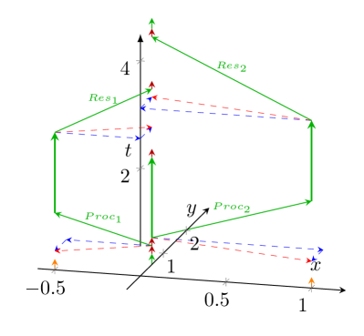
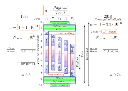
Figure 1: Left: The time diagram of parallelized sequential operation in time-space VeghTemporal:2020 . Right: A conceptual, simplified model VeghScalingANN:2021 of parallelized sequential computing operations, based on their temporal behavior. Notice the different nature of those contributions, and that they have only one common feature: they all consume time.

The non-parallelizable (i.e., apparently sequential) part of tasks comprises contributions from HW, operating system (OS), software (SW) and Propagation Delay (PD), and also some access time is needed for reaching the parallelized system. This separation is rather conceptual than strict, although dedicated measurements can reveal their role, at least approximately. Some features can be implemented in either SW or HW or shared between them. Furthermore, some sequential activities may happen partly parallel with each other. The relative weights of these contributions are very different for different parallelized systems and even, within those cases, depend on many specific factors. In every single parallelization case, a careful analysis is required. SW activity represents what was assumed and discussed by Amdahl as the total sequential fraction. Non-determinism of modern HW systems PerformanceCounter2013  Molnar:2017:Meas also contributes to the non-parallelizable portion of the task: the resulting execution time of parallelly working processing elements is defined by the slowest unit.

Notice that our model assumes no interaction between processes running on the parallelized system and the necessary minimum: starting and terminating otherwise independent processes, which take parameters at the beginning and return their result at the end. It can, however, be trivially extended to more general cases when processes must share some resource (such as a database, which shall provide different records for the different processes), either implicitly or explicitly. Concurrent objects have their inherent sequentiality InherentSequentiality:2012 . Synchronization and communication between those objects considerably increase YavitsMulticoreAmdahl2014 the non-parallelizable portion (i.e. contribution to $(1-\alpha_{eff}^{SW})$ or $(1-\alpha_{eff}^{OS})$) of the task. Because of this effect, in the case of many processors, we must devote special attention to their role in the efficiency of applications on parallelized systems.

The physical size of the computing system also matters. A processor connected to the first one with a cable of dozens of meters must wait for several hundred clock cycles. This waiting is only because of the finite speed of light propagation, topped by their interconnection’s latency time and hoppings (not mentioning geographically distributed computer systems, such as some clouds, connected through general-purpose networks). Detailed calculations are given in Vegh:2017:AlphaEff .

After reaching a certain number of processors, there is no more increase in the payload fraction when adding more processors. The first fellow processor has already finished its task and is idly waiting, while the last one is still idly waiting for its start command. We can increase this limiting number by organizing the processors into clusters: the first computer must speak directly only to the head of the cluster. Another way is to distribute the job near to the processing units. It can happen either inside the processor CooperativeComputing2015 ; DongarraFugakuSystem:2020 , or one can let do the job by the processing units of a GPU .

This looping contribution is not considerable (and, in this way, not noticeable) at a low number of processing units (apart from the other contributions). Still, it can dominate at a high number of processing units. This ”high number” was a few dozens at the time of writing the paper ScalingParallel:1993 , today it is a few millions. We consider the effect of the looping contribution as the borderline between first and second-order approximations in modeling the system’s payload performance. The housekeeping keeps growing with the number of processors, and in contrast, the system’s resulting performance does not increase anymore. The first-order approximation assumes the contribution of housekeeping as constant. The second-order approximation also considers that as the number of processing units grows, housekeeping grows with, gradually becomes the dominating factor of performance limitation, and decreases payload performance.

As Figure 1 shows, in the parallelized operating mode (in addition to computation, furthermore communication of data between its processing units) both software and hardware contribute to the execution time, i.e., they both must be considered in Amdahl’s Law. This finding is not new, again: see AmdahlSingleProcessor67 . Figure 1 also shows where is a place to improve computing efficiency. When combining PD properly with sequential scheduling, one can considerably reduce non-payload time during fine-tuning the system (see the cases of performance increases of $Sierra$ and $Summit$, a half year after their appearance on the TOP500 list). Also, mismatching total time and extended measurement time (or not making a proper correction) may lead to completely wrong conclusions BenchmarkingClouds:2017 as discussed in Vegh:2017:AlphaEff .

3 Amdahl’s Law in terms of our model

Usually, Amdahl’s law is expressed as

$$S^{-1}=(1-\alpha)+\alpha/N$$ (1)

where $N$ is the number of parallelized code fragments (or PU s), $\alpha$ is the ratio of the parallelizable portion to the total, $S$ is the measurable speedup. From this

$$\alpha=\frac{N}{N-1}\frac{S-1}{S}$$ (2)

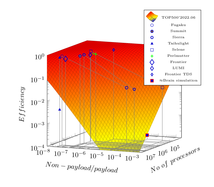
Figure 2: The 2-parameter efficiency surface (in function of parallelization efficiency and number of the processing elements), as concluded from Amdahl’s Law (see Eq. (4)), in first order approximation. Some sample efficiency values for some selected supercomputers are shown, measured with benchmarks HPL and HPCG, respectively. ”This decay in performance is not a fault of the architecture, but is dictated by the limited parallelism” ScalingParallel:1993

When calculating the speedup, one calculates

$$S=\frac{(1-\alpha)+\alpha}{(1-\alpha)+\alpha/N}=\frac{N}{N\cdot(1-\alpha)+\alpha}$$ (3)

hence the resulting efficiency of the system (see Figure 2)

$${\color[rgb]{1,.5,0}\leavevmode\hbox to46.65pt{\vbox to19.07pt{\text{[drawing]}}}}=\frac{S}{N}={\color[rgb]{1,.5,0}\leavevmode\hbox to59.67pt{\vbox to25.85pt{\text{[drawing]}}}}=\frac{R_{Max}}{R_{Peak}} E(\large N,\alpha) \frac{1}{{\color[rgb]{1,0,0}\Large N}\cdot(1-\alpha)+\alpha} E(\large N,\alpha) \frac{1}{{\color[rgb]{1,0,0}\Large N}\cdot(1-\alpha)+\alpha}$$ (4)

This phenomenon itself has been known for decades ScalingParallel:1993 , and $\alpha$ is theoretically established Karp:parallelperformance1990 . Presently, however, the theory was somewhat faded, mainly due to the rapid development of parallelization technology and the increase in single-processor performance.

During the past quarter of a century, the proportion of contributions changed considerably: today the number of processors is thousands-fold higher than a quarter of a century ago. The growing physical size and the higher processing speed increased the role of the propagation overhead, furthermore, the large number of processing units enormously amplified the role of the looping overhead. As a side-result of the technological development, the phenomenon on performance limitation, returned in a technically different form, at a much higher number of processors.

Through using Eq. (4), $E=\frac{S}{N}=\frac{R_{Max}}{R_{Peak}}$ can be equally good for describing the efficiency of parallelization of a setup:

$$\alpha_{E,N}=\frac{E\cdot N-1}{E\cdot(N-1)}$$ (5)

As we discuss below, except for an extremely high number of processors, we can safely assume that the value of $\alpha$ is independent from the number of processors in the system. Eq. (5) can be used to derive the value of $\alpha$ from values of parameters $R_{Max}/R_{Peak}$ and the number of cores $N$.

According to Eq. (4), the payload efficiency can be described with a 2-dimensional surface, as shown in Figure 2. On the surface, we displayed some measured efficiencies of the current top supercomputers to illustrate some general rules. Both the HPL and the HPCG efficiency values are displayed. We project the measured values back to the axes to enable the reader to compare the corresponding values of their number of processors and parallelization efficiency. The HPL efficiency sharply decreases with the increasing number of cores in the system. In the case of unnaturally high (or not provided) HPCG efficiency values, the values are not displayed in the figure. The last ”world champion” which benchmarked HPCG correctly was $Taihulight$.

We can divide the measured values into two groups. The first group comprises measurements where the same number of cores were used in both benchmarks. For visibility, only the HPL projections are displayed, and on their top, the HPCG data point. The general experience showed that the ratio of HPL-to-HPCG efficiency is about 200-500 when using the same number of cores. The HPCG payload performance reached its ”roofline” WilliamsRoofline:2009  VeghScalingANN:2021 level at a lower number of cores; using all cores would decrease the system’s performance because of the higher number of cores. This issue is why the members of the second group reduced their number of cores in the HPCG benchmark.

The recent trend is that only a tiny fraction (only about 10 %) of supercomputer’s cores are used in the HPCG benchmarking, while all cores are used in the HPL benchmarking. Beginning with June 2021, the data ”Measured cores” are not provided anymore, covering this aspect. The presumable reason is that in this way the measured HPCG/HPL efficiency ratio gets much higher, providing the illusion that the vast supercomputers became more suitable for real-life tasks. The supercomputers based on the newly developed AMD EPYC 7763 64C processors also did not provide their HPCG efficiency and performance, or they provide an incorrect number of measured cores.

There is an inflection point in the performance: ”there comes a point when using more PU s …actually increases the execution time rather than reducing it” ScalingParallel:1993 . We can observe a quick breakdown of the performance gain as theoretically predicted VeghScalingANN:2021 and experimentally measured, see AngeloLearningBioinformatics:2014 (Fig. 13) or NeuralScaling2017 (Fig. 7). As can be concluded from the figure, increasing the systems’ nominal performance by order of magnitude, at the same time, decreases its efficiency (and so: its payload performance) by more than an order of magnitude.

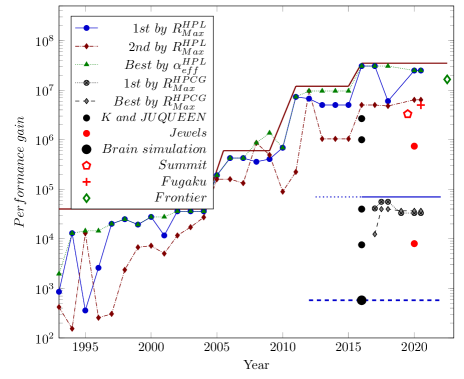
Figure 3: The performance gain of top supercomputers, in function of their year of production. The marks display the measured values derived using HPL and HPCG benchmarks, for the TOP3 supercomputers. The small black dots mark the performance data of supercomputers $JUQUEEN$ and $K$ as of 2014 June, for HPL and HPCG benchmarks, respectively. The big black dot denotes the performance value of the system used by NeuralNetworkPerformance:2018 . The red pentagons denote performance gain, measured using half-precision operands. The saturation effect can be observed for both HPL and HPCG benchmarks.

The goal of the Gordon Bell Prize GordonBellPrize:2017 was originally ”to demonstrate a speedup of at least 200 times on a real problem”, and the community noticed a decade ago that the efficacy measured with the benchmark HPL and that of the real-life applications started to differ by up to two orders of magnitude. It would be worth recalling that the new benchmark program HPCG HPCGB:2015 was introduced since ”HPCG is designed to exercise computational and data access patterns that more closely match a different and broad set of important applications, and to give incentive to computer system designers to invest in capabilities that will have impact on the collective performance of these applications” HPCG_List:2016 . The present design efforts target building ”racing” computers, and the constructors either do not publish their HPCG efficiency or measure it using only a fraction (about 10 %) of their cores. The developers aim to produce higher figures by the HPL benchmark instead of making higher performance in the real-life-imitating HPCG benchmark. It is simply misleading to claim that building such racing supercomputers ”will enable scientists to develop critically needed technologies for the country’s energy, economic and national security, helping researchers address problems of national importance that were impossible to solve just five years ago” and that ”Scientists and engineers from around the world will put these extraordinary computing speeds to work to solve some of the most challenging questions of our era” ORNLFrontier:2022 .

Comments such as ”The HPCG performance at only 0.3% of peak performance shows the weakness of the Sunway TaihuLight architecture with slow memory and modest interconnect performance” DongarraSunwaySystem:2016 and ”The HPCG performance at only 2.5% of peak performance shows the strength of the memory architecture performance” DongarraFugakuSystem:2020 show that supercomputing experts did not realize, that the efficiency is a(n at least) 2-parameter function, depending on both the number of PU s in the system and its workload; furthermore, that the workload defines the achievable payload performance. It looks like the community experienced the effect of the two-dimensional efficiency but did not want to comprehend its reason, despite the early and clear prediction: ”this decay in performance is not a fault of the architecture, but is dictated by the limited parallelism” ScalingParallel:1993 . In excessive systems of modern HW, it is also dictated by the laws of nature VeghModernParadigm:2019 . Furthermore, we can perfectly describe its dependence by the correctly interpreted Amdahl’s Law, rather than being ”empirical efficiency”.

Notice two more rooflines. During the development of the interconnection technology, between the years 2004 and 2012, different implementation ideas have been around, and they competed for years. The beginning of the second roofline, around the year 2011, coincides with the dawn of GPU s, interfering with the effect of the interconnection technology; see also section 4.3.

The top roofline dawned with the appearance of $Taihulight$: some assistant processors take over part of the duties of the individual cores, and in this way, one can mitigate the non-payload portion of the workload. This roofline can be slightly above the possible roofline at the price of using a slightly modified computing paradigm; using cooperating cores.

It is important to notice the two red pentagons in the figure: they represent the performance gain achieved using half-precision operand length. The performance gain is lower than the double precision equivalent, just because of the increased relative weight of housekeeping, as discussed in detail in section 4.5.

The projections of efficiency values to axes show that the top few supercomputers offer similar parallelization efficiency and core number values; both features are required to receive one of the top slots. Supercomputers $Taihulight$ and $Fugaku$ are exceptions on both axes. They have the highest number of cores and the best $HPL$ parallelization efficiency. An interesting coincidence is that the processors of both supercomputers have ”assistant cores” (i.e., some cores do not make payload computing; instead, they take over ”housekeeping duties”). This solution makes housekeeping in parallel with the payload computing (reduces the sequential portion of the task) and, in this way, decreases the internal latency of processors making payload computing and increases the system’s efficiency. They both use a ”light-weight operating system” (and so do $Fugaku$, $Summit$ and $Sierra$) to reduce processor latency. This efficiency, of course, requires executing several floating instructions per clock cycle. That mode of operation gets more and more challenging for the interconnection, delivering data to and from data processing units. Notice also in their cases the role of ”near” memories: as explained in VeghTemporal:2020 , the data delivery time considerably increases the ”idle time” of computing. This idle time is why $Fugaku$, with its cleverly placed $L_{2}$ cache memories, can be more effective when measured with HPL. However, this trick does not work in the case of $HPCG$ because its ”sparse” computations use those cache memories ineffectively. We expect the ”true” $HPCG$ efficiency of $Fugaku$ to be between the corresponding values of $Summit$ and $Taihulight$.

The newly (as of 2022) developed AMD EPYC 7763 64C processors did not cause a revolution. On the one side, they introduced a performance jump, quite similarly to the appearance of the NVidia accelerators some years ago. On the other side, their internal latency allowed to achieve a somewhat higher performance gain. As the data point representing $Frontier$ shows, their performance gain is slightly higher than that of systems without acceleration and considerably higher than that of systems having accelerators with non-shared data space. However, they did not require developing new theoretical approach.

The processors of $Taihulight$ comprise cooperating cores CooperativeComputing2015 . The direct core-to core transfer uses a (slightly) different computing paradigm: the processor cores explicitly assume the presence of another core, and in this way, their effective parallelism becomes much better, see also Fig. 6. On that figure, this data and the ones using shorter operands ($Summit$ and $Fugaku$) result in performance values above the limiting line. However, reducing the loop count by internal clustering (in addition to the ”hidden clustering”, enabled by its assistant cores) and exchanging data without using the global memory works only for the $HPL$ case, where the contribution of SW is low. The poor value of $(1-\alpha_{eff}^{HPCG})$ is not necessarily a sign of architectural weakness NSA_DOE_HPC_Report_2016 : $Taihulight$ comprises about four times more cores than $Summit$ and performs the HPCG benchmark with ten-fold more cores. Given that HPCG mimics ”real-life” applications, one can conclude that for practical purposes, only systems comprising a few hundred thousand cores shall be built, see also section 4.4. More cores contribute only to the ”dark performance”.

According to Eq. (4), efficiency can be interpreted in terms of $\alpha$ and $N$, and the efficiency of a parallelized sequential computing system can be calculated as

$$P(N,\alpha)=\frac{N\cdot P_{single}}{{N\cdot\left(1-\alpha\right)+\alpha}}$$ (6)

This simple formula explains why the payload performance is not a linear function of the nominal performance and why in the case of very good parallelization ($(1-\alpha)\ll 1$) and low $N$, this nonlinearity cannot be noticed.

The value of $\alpha$, however, can hardly be calculated for the present complex HW/SW systems from their technical data (for a detailed discussion see VeghScalingANN:2021 ). We can follow two ways to estimate their value of $\alpha$. One way is to calculate $\alpha$ for existing supercomputing systems (making ”computational experiments”AmdalVsGustafson96 ) applying Eq. (5) to data in TOP500 list VeghModernParadigm:2019 . This way provides a lower bound, already achieved, for $(1-\alpha)$. Another way round is to consider contributions of different origins, see section 4, and to calculate the high limit of the value of $(1-\alpha)$, that the given contributions alone do not enable to exceed (provided that that contribution is the dominant one). It gives us good confidence in the reliability of the parameters that the values derived in these two ways differ only by up to a factor of two. At the same time, this also means that technology is already very close to its theoretical limitations.

Notice that the ”algorithmic effects” – such as dealing with ”sparse” data structures (which affects cache behavior, which will have a growing importance in the age of ”real-time everything”, ”big data”, and ”neural networks”) or communication between parallelly running threads, such as returning results repeatedly to the main thread in an iteration (which greatly increases the non-parallelizable fraction in the main thread) – manifest through the HW/SW architecture, and we can hardly separate them. Also notice that there are one-time and fixed-size contributions, such as utilizing time measurement facilities or calling system services. Since $\alpha_{eff}$ is a relative merit, the absolute measurement time shall be large. When utilizing efficiency data from measurements dedicated to some other goal, we must exercise proper caution with the interpretation and accuracy of those data.

The ’right efficiency metric’ EfficiencyMetric:2012 has always been a question (for a summary see cited references in HSWscalable2012 ) when defining efficient supercomputing. The present discussion aims to discover the inherent limitations of parallelized sequential computing and provide numerical values. For this goal, the ’classic interpretation’ AmdahlSingleProcessor67 ; ScalingParallel:1993 ; Karp:parallelperformance1990 of performance was used, in its original spirit. We scrutinized the contributions mentioned in those papers and revised their importance under current technical conditions.

4 The effect of different contributions to $\alpha$

Theory can display data from systems with any contributors with any parameters. From measured data, we can conclude only the sum of all contributions, although dedicated measurements can reveal the value of separated contributions experimentally. The publicly available data enable us to conclude mainly of limited validity.

4.1 Estimating different limiting factors of $\alpha$

The estimations below assume that the actual contribution is the dominating one, which defines the achievable performance alone. This situation is usually not the case in practice (the convolution of different contributions is limiting), but this approach enables us to find out the limiting $(1-\alpha)$ values for all contributions.

In the systems implemented in Single Processor Approach (SPA) AmdahlSingleProcessor67 as parallelized sequential systems, the life begins and ends in one such sequential subsystem, see also Fig. 1. In large parallelized applications, running on general-purpose supercomputers, initially and finally, only one thread exists, i.e., the minimal necessary non-parallelizable activity is to fork the other threads and join them again.

With the present technology, no such actions can be shorter than one processor clock period. The theoretical absolute minimum value of the non-parallelizable portion of the task will be given as the ratio of the time of the two clock periods to the total execution time. The latter time is a free parameter in describing efficiency. That is, the value of effective parallelization $\alpha_{eff}$ depends on the total benchmarking time (and so does the achievable parallelization gain, too).

This dependence, of course, is well known for supercomputer scientists. For measuring the efficiency with better accuracy (and also for producing better $\alpha_{eff}$ values), one uses hours of execution times in practice. In the case of benchmarking supercomputer $Taihulight$ DongarraSunwaySystem:2016 , 13,298 seconds HPL benchmark runtime was used; on the 1.45 GHz processors it means $2*10^{13}$ clock periods. The inherent limit of $(1-\alpha_{eff})$ at such benchmarking time is $10^{-13}$ (or, equivalently, the achievable performance gain is $10^{13}$). For simplicity, in the paper, 1.00 GHz processors (i.e., 1 ns clock cycle time) will be assumed.

Supercomputers are also distributed systems. In a stadium-sized supercomputer, we can assume a distance between processors (cable length) up to about 100 m. The net signal round trip time is ca. $10^{-6}$ seconds, or $10^{3}$ clock periods, i.e., in the case of a finite-sized supercomputer, the performance gain cannot be above $10^{10}$, only because of the physical size of the supercomputer. The presently available network interfaces have 100…200 ns latency times and sending a message between processors takes time in the same order of magnitude, typically 500 ns. This timing also means that making better interconnection is not a bottleneck in enhancing performance. This statement is also underpinned by the discussion in section 4.3. However, sharing data instead of copying them, can result in demonstrative performance improvements, see the case of $Frontier$.

These predictions enable us to assume that the presently achieved value of $(1-\alpha_{eff})$ could also persist for roughly a hundred times more cores. However, another major issue arises from the computing principle SPA: the first processor can address only one processor at a time. As a consequence, at least as many clock cycles are to be used for organizing the parallelized work as many addressing steps are required. This number equals the number of cores in the supercomputer, i.e., the addressing operation in supercomputers in the TOP10 positions typically needs clock cycles in the order of $5*10^{5}$…$10^{7}$; degrading the value of $(1-\alpha_{eff})$ into the range $10^{-6}$…$2*10^{-5}$. One can use two tricks to mitigate the number of the addressing steps: either cores are organized into clusters as many supercomputer builders do, or at the other end, the processor itself can take over the responsibility of addressing its cores CooperativeComputing2015 . In function of the actual construction, the reducing factor of clustering of those types can be in the range $10^{1}$…$5*10^{3}$, i.e the resulting value of $(1-\alpha_{eff})$ is expected to be around $10^{-7}$.

As Eq. (6) suggests, the trivial way to increase systems’ performance is to improve a single processor’s performance; for example, combining the PU s with accelerators. Various implementations of the idea exist, but ”What is initially perplexing is that accelerators do not dominate the architectures in the Top500, given the performance and price/performance advantages they offer as compute engines” NextPlatformHPCExascaleBarrier:2022 . This situation seems to change: now the Frontier has taken over the leading position, and presumably, other supercomputers will be built with its technology. The primary reason for the change is that sharing data (mainly at $L_{1}$ and $L_{2}$ levels), as opposed to copying data between the separated address fields of PU and GPU, dramatically reduces the internal latency of the PU s, and in the case of ”racing” supercomputers, this non-payload contribution can be decisive, see section 4.2. A critical difference between the previous and recent designs of GPU s is that ”The two GK110 GPUs in the K80s were not interconnected and could not share data; the two Aldebaran GCDs are and can.” NextPlatformAMDAldebaran:2022 ”. The consequence of the lower latency is a higher performance gain and, due to it, a higher absolute performance. The former GPU s, because of their higher latency due to copying between address spaces, could not get into the top group of supercomputers.

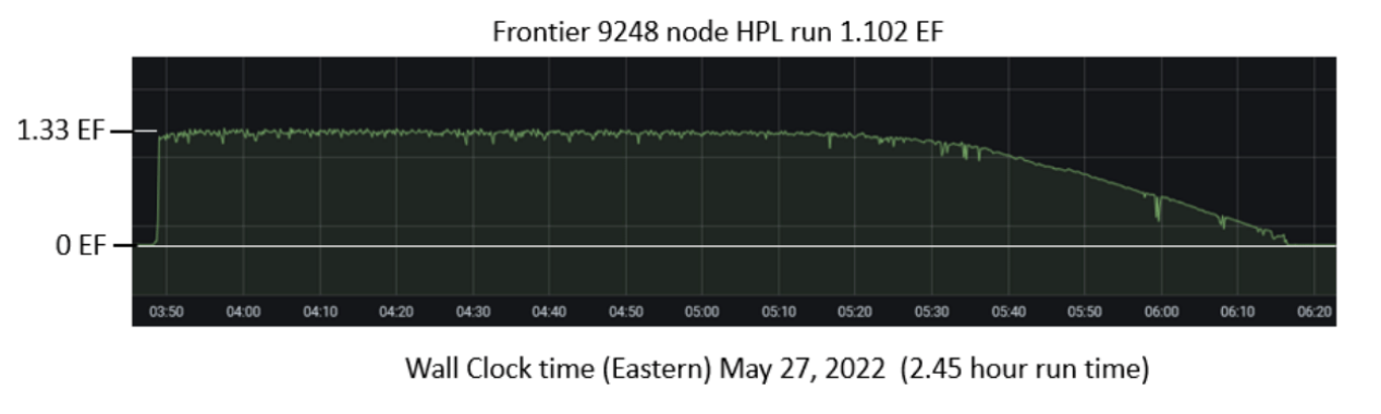
Figure 4: The time dependence of the number of floating point operations performed when running benchmark HPL on supercomputer Frontier. Reproduced from FrontierHPCwire:2022

NextPlatformFrontierStepByStep:2022 introduces an unexplained claim: ”As configured for the Linpack run, the Frontier system had a power draw of 21.1 megawatts, but …when the Frontier machine is first set loose on the Linpack, it draws an extra 15 megawatts of power as it is starts the job.” Together with Fig. 4 one can understand why.

At the very beginning and end of computation, the operands shall be distributed and results collected, respectively. This non-payload contribution grows with the number of cores. As discussed above, several ideas are used to reduce its time: from the very common ”clustering” to using assistant cores CooperativeComputing2015 . Frontier introduced a revolutionary solution for that task. As the left side of Fig. 4 illustrates, for about 3 minutes, Frontier, at least its monitored part, does not perform floating operations. After that period, all operands suddenly appear in their place, and the supercomputer can make its computations at full speed; apparently, no time is spent transferring the operands to the peer cores. This task is what Frontier uses the extra 15 MW power for; for this short period, a hidden second specialized supercomputer starts up, with the only mission to deliver the operands to their place. From the viewpoint of the coordinator core, it is read-only access that can be massively parallelized. However, it needs a terrible parallel bus capacity and electric power to drive millions of Input/Output (I/O) ports.

The right side of Fig. 4 illustrates that when the benchmark computation HPL finishes, it takes about 40 minutes to collect the data from its nearly 9M cores. It enables us to estimate also that the value of $T_{T}$ (the time needed for a single transfer) is about $200,000\ ns$ FrontierHPCwire:2022 ; a value unexpectedly high compared to Slingshot’s advertised 200 Gb/sec transfer bandwidth. The issue shows a very poor bus utilization. The datasheet value does not consider the arbitration time and data transmission time. This finding is not unprecedented: NextPlatformHPCExascaleBarrier:2022 mentions that ”IBM and Nvidia had issues with the NVLink coherent fabric between the CPUs and GPUs in Summit, and that machine did not get 200 Gb/sec InfiniBand as was hoped when it was installed.” Yes, the ”proxy” core and the separated CPU/GPU address space increased the node’s internal latency (its non-payload contribution).

The figure also shows that the submitted computing performance is averaging the momentary values for the period shown in the figure. Without the ”phantom supercomputer” (i.e., having two ramps), the performance would be about 0.8 EFlops (that is, less than the magic 1 EFlops), and with a sufficiently long measurement time, it could approach 1.3 EFlops. Notice that the ”ramp” on the right side would occur several times in HPCG-type computations (and, of course, in all real-life computations) would keep the average computing performance low. To prevent this, one can reduce the number of the measured cores to, say, 10%, in which case the ramp’s length is about 4 minutes, and in that way, much better efficiency and speedup can be reported.

The ’end of computation’ situation means that the orchestrating core must collect the result from all peer cores. It imitates the case when in an Artificial Intelligence (AI) workload a ’neuron’ must collect the results from all of its (interested) peers, and all neurons want to make that action at the same time, using the same single bus. For a AI-type application, the increased level of communication keeps PU s waiting for the single high-speed bus so that the computed results ”are processed as they come in”, and to reduce the apparent overload, ”are dropped if the receiving process is busy over several delivery cycles” NeuralNetworkPerformance:2018 . Actually, using a single high-speed bus excludes the chance of achieving a real-time simulation speed. This method of implementation is why ”artificial intelligence, …it’s the most disruptive workload from an I/O pattern perspective”.

One must also use an operating system for protection and convenience. If fork/join is executed by the OS as usual, because of the needed context switchings $2*10^{4}$ Tsafrir:2007 ; armContextSwitching:2007 clock cycles are used, rather than 2 clock cycles considered in the idealistic case. The derived values are correspondingly by four orders of magnitude different, that is, the absolute limit is $\approx~{}5*10^{-8}$, on a zero-sized supercomputer. This value is somewhat better than the limiting value derived above, but it is close to that value and surely represents a considerable contribution. This limitation is why a growing number of supercomputers uses ”light-weight kernel” or runs its actual computations in kernel mode; a method of computing that we can use only with well-known benchmarks. Frontier’s ’phantom supercomputer’ eliminates also this OS contribution.

However, this optimistic limit assumes that the processor can access its instructions in one clock cycle. It is usually not the case, but it seems to be a good approximation. On the one side, even a cached instruction in the memory needs about five times more access time and the time required to access ’far’ memory is roughly 100 times longer. Correspondingly, the optimistic achievable performance gain values shall be scaled down by a factor of $5\dots 100$. A considerable part of the difference between efficiencies $\alpha_{eff}^{HPL}$ and $\alpha_{eff}^{HPCG}$ can be attributed to a different cache behavior because of the ’sparse’ matrix operations.

4.2 The effect of workload

The overly complex Figure 5 attempts to explain the phenomenon, why and how the performance of a supercomputer configuration depends on the application it runs. The non-parallelizable fraction (denoted in the figure by $\alpha_{eff}^{X}$) of the computing task comprises components $X$ of different origins. As we already discussed and was noticed decades ago, ”the inherent communication-to-computation ratio in a parallel application is one of the important determinants of its performance on any architecture” ScalingParallel:1993 , suggesting that communication can be a dominant contribution in system’s performance. Figure 5.A displays a case with minimum communication, and Figure 5.B a case with moderately increased communication (corresponding to real-life supercomputer tasks). As the nominal performance increases linearly and the payload performance decreases inversely with the number of cores, at some critical value, where an inflection point occurs, the resulting payload performance starts to drop. The resulting non-parallelizable fraction sharply decreases the efficacy (or, in other words: performance gain or speedup) of the system VeghPerformanceWall:2019 ; VeghBrainAmdahl:2019 . The effect was noticed early ScalingParallel:1993 , under different technical conditions, but somewhat faded due to successes of development of parallelization technology.

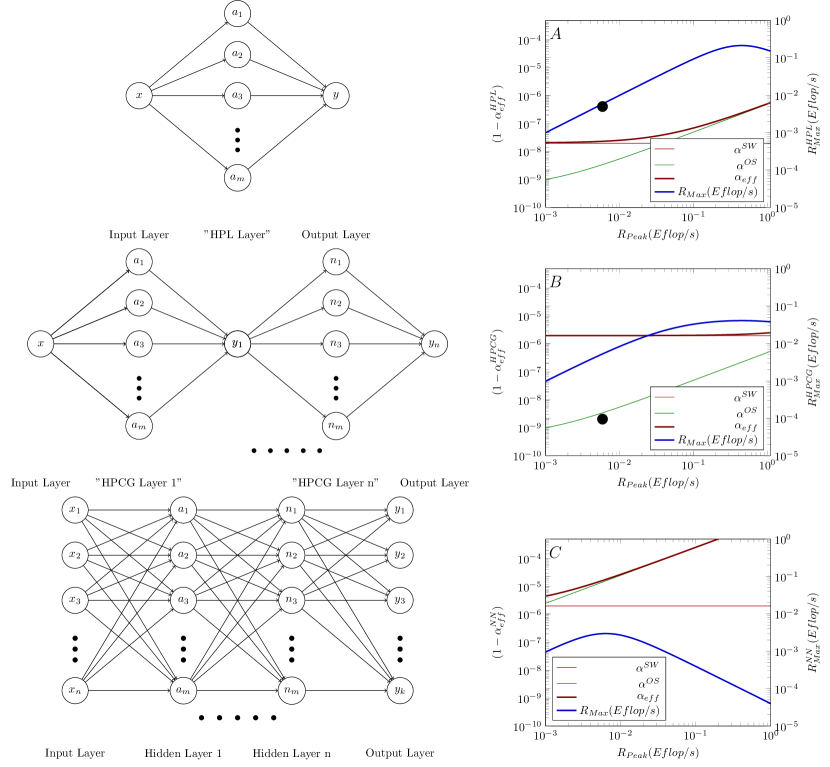
Figure 5: The figure explains how the different communication/computation intensities of applications lead to different payload performance values in the same supercomputer system. Left column: models of the computing intensities for different benchmarks. Right column: the corresponding payload performances and $\alpha$ contributions in function of the nominal performance of a fictive supercomputer ($P=1Gflop/s$ @ $1GHz$). The blue diagram line refers to the right hand scale ($R_{Max}$ values), all others ($(1-\alpha_{eff}^{X})$ contributions) to the left hand scale. The figure is purely illustrating the concepts; the displayed numbers are somewhat similar to real ones. The performance breakdown shown in the figures were experimentally measured by ScalingParallel:1993 ,  NeuralScaling2017 (Figure 7) and NeuralNetworkPerformance:2018 (Figure 8).

Figure 5.A illustrates the behavior measured with HPL benchmark. The looping contribution becomes remarkable around 0.1 Eflops, and breaks down payload performance (see Figure 1 in ScalingParallel:1993 ) when approaching 1 Eflops. In Figure 5.B, the behavior measured with benchmark HPCG is displayed. The application’s contribution (brown line) is much higher than in the previous case. The looping contribution (thin green line) is the same as above. Consequently, the achievable payload performance is lower, and the payload performance breakdown is softer in the case of real-life tasks.

Figure 3 depicts the experimental equivalent of Figure 5. Given that no dedicated measurements exist, it is hard to compare theoretical prediction directly to measured data. However, the impressive and quick development of interconnecting technologies provides a helping hand.

In the HPL class, the communication intensity is the lowest possible one: the computing units receive their task (and parameters) at the beginning of the computation, and they return their result at the very end. The core orchestrating their work must only deal with the fellow cores in these periods, so their communication intensity is proportional to the number of cores in the system. Notice the need to queue requests at the task’s beginning and end.

In the HPCG class, iteration takes place: the cores return the result of one iteration to the coordinator core, which makes sequential operations: not only receives and re-sends parameters but also needs to compute new parameters before sending them to the fellow cores. The program repeats the process several times. As a consequence, the non-parallelizable fraction of the benchmarking time grows proportionally to the number of iterations and the size of the problem. The effect of that extra communication decreases the achievable performance roofline WilliamsRoofline:2009 : as shown in Fig. 3, the HPCG roofline is about 200 times smaller than the HPL one, as discussed in section 3. Turning the memory into (partly) active elements, using different ’coherence’ solutions such as OpenCAPI OpenCAPI:2019 or data sharing at levels $L_{1}$ and $L_{2}$, can mitigate this effect. See also section 5.

4.3 The effect of interconnection

As discussed above, in a somewhat simplified view, we can calculate the resulting performance using the contributions to $\alpha$ as

$$P(N,\alpha)=\frac{N\cdot P_{single}}{{\color[rgb]{1,0,0}N}\cdot\left(1-{\color[rgb]{1,0,0}\alpha_{Net}-\alpha_{Compute}}-\alpha_{Others}\right)+\approx 1}$$ (7)

That is, we must handle two of the contributions with emphasis. The theory provides values for contributions of interconnection and calculation separately. Fortunately, the public database TOP500 TOP500 also provides data measured under conditions considerably similar to measure the ’net’ interconnection contribution. Of course, the measured data reflect the sum of contributions of all components. However, as will be shown below, in the total contribution, those mentioned contributions dominate, and all but the contribution from networking are (nearly) unchanged, so the difference of measured $\alpha$ can be directly compared to the difference of the corresponding sum of calculated $\alpha$ values, although here only qualitative agreement can be expected.

Both the quality of the interconnection and the nominal performance are a parametric function of their construction time. One can assume on the theory side that (in a limited period), interconnection contribution was changing in the function of nominal performance as shown in Figure 6A. The other primary contribution is assumed to be computation itself. Benchmark computation contributions for HPL and HPCG are very different, so the sum of the respective component plus the interconnection component is also very different. Given that at the beginning of the considered period, the contribution from the HPCG calculation and that of the interconnection was in the same order of magnitude, their sum only changed marginally (see the upper diagram lines), i.e., the measured performance improved only slightly. Because the benchmark HPCG is communication-bound (and so are real-life programs), their efficiency would be an order of magnitude worse. The reason is Eq. (4): when supercomputers use all of their cores, their achievable performance is not higher (or maybe even lower), only their power consumption is higher (and the calculated efficiency is lower). As predicted: ”scaling thus put larger machines at an inherent disadvantage” ScalingParallel:1993 . The cloud-like supercomputers have a disadvantage in the HPCG competition: the Ethernet-like operation results in relatively high $(1-\alpha)$ values.

The case with HPL calculation is drastically different (see the lower diagram lines). In this case, at the beginning of the considered period, the contribution from interconnection is very much larger than that from the computation. Consequently, the sum of these two contributions changes sensitively as the speed of the interconnection improves. As soon as the contribution from interconnection decreases to a value comparable with that from the computation, the decrease of the sum slows down considerably, and further improvement of interconnection causes only marginal decrease in the value of the resulting $\alpha$ (and so only a marginal increase in the payload performance).

The measured data enable us to draw the same conclusion, but one must consider that here multiple parameters may have changed. Their tendency, however, is surprisingly straightforward. Figure 6.B is actually a 2.5D diagram: the size of marks is proportional to the time passed since the beginning of the considered period. A decade ago, the speed of interconnection gave a significant contribution to $\alpha_{total}$. Enhancing it drastically in the past few years increased systems’ efficacy. At the same time, because of the stalled single-processor performance, the other technology components changed only marginally. The computational contribution to $\alpha$ from benchmark HPL remained constant in the function of time, so the quick improvement of the interconnection technology resulted in a quick decrease of $\alpha_{total}$, and the relative weights of $\alpha_{Net}$ and $\alpha_{Compute}$ reversed. The decrease in the value of $(1-\alpha)$ can be considered as the result of the decreased contribution from interconnection.

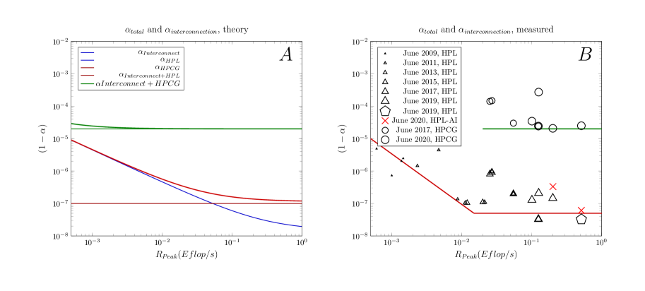
Figure 6: The effect of changing the dominating contribution. The left subfigure shows the theoretical estimation, the right subfigure the corresponding measured data, as derived from public database TOP500 TOP500 (only values for the first four supercomputers are shown). When the contribution from interconnection drops below that of computation, the value of $(1-\alpha)$ (and the performance gain) get saturated. The red ’x’ marks denote half-precision values.

However, the total $\alpha$ contribution decreased considerably only until $\alpha_{Net}$ reached the order of magnitude of $\alpha_{Compute}$. This match occurred in the first 4-5 years of the period shown in Figure 6B: the sloping line is due to the enhancement of interconnection. Then, the two contributors changed their role, and the constant contribution due to computation started to dominate, i.e., the total $\alpha$ contribution decreased only marginally. As soon as the computing contribution took over the dominating role, the value of $\alpha_{total}$ did not fall anymore: all measured data remained above that value of $\alpha$. Correspondingly, the payload performance improved only marginally (and due to factors other than interconnection).

At this point, as a consequence of that the dominating contributor changed, it was noticed that the efficacy of benchmark HPL and the efficacy of real-life applications started to differ by up to two orders of magnitude. Because of this, a new benchmark program HPCG HPCGB:2015 was introduced, since ”HPCG is designed to exercise computational and data access patterns that more closely match a different and broad set of important applications” HPCG_List:2016 .

Since the major contributor is the computing itself, the different benchmarks contribute differently, and since that time the ”supercomputers have two different efficiencies” DifferentBenchmarks:2017 . Yes, if the dominating $\alpha$ contribution (from the benchmark calculation) is different, then the same computer shows different efficiencies in the function of the computation it runs. Since that time, the interconnection provides less contribution than the computation of the benchmark. Due to that change, enhancing the interconnection contributes mainly to the dark performance, rather than to the payload performance. For the goals of exascale computing, the efforts (and expenses) to enhance interconnection seem to be rather pointless. For today, even in the benchmark HPL, the sequential contribution of interconnection is only a tiny fraction of the computation itself; for solving real-life problems, enhanced interconnection makes no noticeable difference. The fundamental issue is that the need for communication (including ”sparse” computations) blocks computing performance.

Figure 7: Correlation of performance of processors using accelerator with separate address space and effective parallelism with ranking, in 2017.

4.4 The effect of accelerator

As suggested by Equ. (6), the trivial way to increase supercomputers’ resulting payload performance is to increase the single-processor performance of its processors. Given that the single processor performance has reached its limitations, some accelerators are frequently used for this goal. Fig. 7 shows how using accelerators with separate address space influences ranking of supercomputers.

The left subfigure shows that supercomputers’ ranking does not depend on which acceleration method it uses. Essentially the same is confirmed by the right subfigure: the non-payload portion raises with the ranking position, and the slope is the same for any acceleration. As the left subfigure depicts, GPU-accelerated processors increase the payload performance of the system by a factor of 2-2.5 (the value is in good accordance with that measured in Lee:GPUvsCPU2010 ). The right subfigure discovers that the non-payload to payload ratio of GPU-accelerated systems is nearly an order of magnitude worse than that of the non-accelerated systems. That is, the resulting efficiency can be (depending on the size of the system) worse than in the case of utilizing unaccelerated processors; this can be a definite disadvantage when GPU s used in a system with a vast number of processors. See also section 5, on the one side, how introducing GPU s to the system increased their payload performance; on the other side, how changing GPU to another type, with a higher nominal performance, but larger memory to be filled with copied content, affected payload performance of the system.

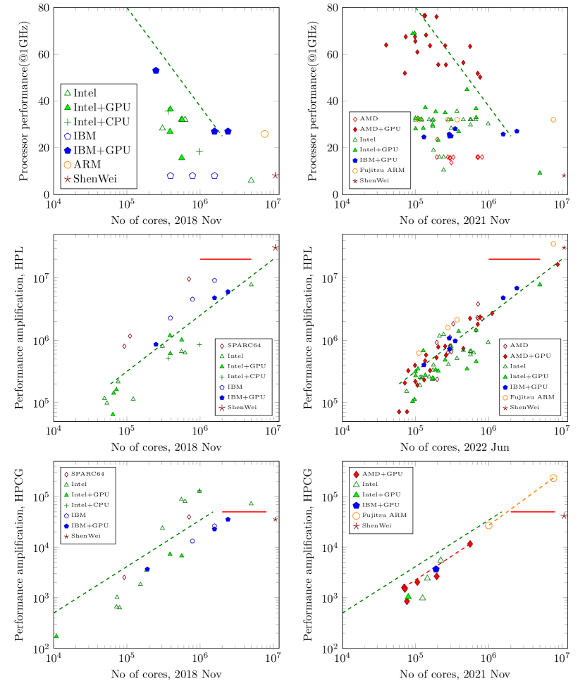
Figure 8: The correlation of the specific single processor performance (top row) and non-payload to payload efficiency (middle row: HPL, bottom row: HPCG) with the number of cores in the system. The empty figures mark non-accelerated, and the filled figures GPU accelerated processor systems. The present (as of November 2021) state (right column) versus the state three years ago (left column). The red line section displays the estimated theoretically possible best non-payload to payload ratio (see section 4.1). The dashed line serves as a guide for the eye.

The ’weak scaling’ provides a quick and easy way to estimate the nominal performance of a designed system. However, we experience an empirical efficiency, see Fig. 2, when measuring actual systems’ payload performance, which refutes the validity of ’weak scaling’. With the proliferation of supercomputers using the same GPU-accelerator and based on the same processor in systems of various sizes, we can refute the fallacy that an added GPU accelerator multiplies the payload performance of the system’s cores by the nominal performance of the GPU. At the same time, we can more safely estimate the final empirical limits of supercomputing (using the present computing paradigm).

Fig. 8 shows how the specific single-processor performance (the single processor performance divided by the clock frequency) and the non-payload to payload ratio change in the function of the number of system’s cores. The figures also show how a better integration with the GPU components (and the intention to achieve higher performance) transformed the landscape in three years.

As the top row displays, the accelerated specific processor performance (unlike power consumption) decreases to the level of non-accelerated specific processor performance as the systems’ size increases. We could guess this tendency already three years ago, but now it has become much more expressed with the appearance of masses of GPU-accelerated systems. On the one side, the enhanced acceleration technology is susceptible to the implementation method (shows a significant variance), but it can produce a performance boost factor of about 4. The dedicated measurements provided a factor 2…3 only Lee:GPUvsCPU2010 but in some implementations of supercomputers, the enhancement is marginal (see the upper left subfigure of Fig. 8). On the other side, the required non-payload to payload ratio strongly decreases as the number of the cores in the system increases (also reflecting the effect of the physical size); and it is different for different workloads.

As the middle and bottom rows display, using an accelerator seems not to influence how the amplification factor depends on the number of cores: the increased latency (caused by the need to copy data between the address spaces) counterbalances the higher processor performance at those core numbers. In the case of the benchmark HPL, the dashed line (serving to guide the eye) crosses the estimated performance limit (the short red line section, see subsection 4.1) at about 10M. Its meaning is that this could be the maximum number of cores that can cooperate in the case of this workload. In the case of the benchmark HPCG, the performance roofline is about 200 times lower, and the critical number of cores has a ten times lower value. The red diamonds impressively populated the figure, but they all belong to a relatively low number (a few hundred thousand) of cores. There is no chance they can work with cores above a million. The right subfigures underpin that a high number of processors must be accompanied with good parallelization efficiency. Otherwise, the large number of cores cannot counterbalance the decreasing efficiency, see Eq. (6). We cannot build more extensive systems using the present paradigm and technology.

The two measured data points above the rooflines mark the supercomputers Fugaku and Taihulight. The latter uses ’cooperating processors’ CooperativeComputing2015 ; both are slightly deviating from the classic computing paradigm. The former can perform better because of the cleverly placed cache memories (closer to the ’in-memory computing’). We can increase the nominal performance without limitation. Still, the system either will not start up at all (mainly because of the ”communication collapse” CommunicationCollapse:2018 ) or will work only at marginal computing and energetic efficiency. For the HPCG workload, because of the reasons mentioned, only reliable data are included.

Noticeably, in Fig. 2 the systems having the best efficiency values do not use accelerator: the efficiency of systems using accelerators is much lower also in the case of HPL benchmark, but it is more disadvantageous in the case of HPCG benchmark. As can be seen, one can reach the ”roofline” efficiency with using only a fragment of the available cores. The two new items in Fig. 2 (as of June 2021, Selene and Jewels; based on entirely GPU s) not only show the worst efficacy for HPL benchmark, but their HPCG efficiencies push back the number of usable cores (for real-life tasks) well below the hundred thousand limit. On the one side, the achieved HPCG efficiency values show the same tendency as the HPL efficiency values: the more cores, the lower efficiency. On the other side, figures 2 and 8 show that for real-life tasks, the reasonable size of supercomputers (even in the case of benchmark HPL) is below 1M core for non-accelerated cores. At that number of cores, their efficiency is just a few percent, and increasing the number of cores decreases their efficiency (does NOT increase their payload performance). In other words, we can conclude that the accelerators enable the systems to reach a much worse non-payload to payload ratio. For an example, see Perlmutter. The slight increase in both the nominal and payload performance for benchmark HPL (the HPL roofline reached) is not accompanied by any enhancement for benchmark HPCG (the HPCG roofline already arrived at a small fragment of cores).

In the past few years, there has appeared the tendency to attempt to show up better efficiency values when excessive supercomputers attack real-life tasks; the right bottom figure shows why. The theoretically estimated amplification factor is about 200-300 times lower for the HPCG workload than that for the HPL workload. However, some HPCG data points seem to appear with a much better amplification factor. The reason is that the HPCG workload does not enable to increase the system’s payload performance above its roofline when using the same number of cores that were used when benchmarking the systems with HPL workload. Because of this limitation, the ”measured cores” in the HPCG benchmarking is just a fragment (about 10 %) of the total cores. The figure shows two connected data point pairs. The upper point is the published performance (calculated assuming that the total number of cores was used) the lower point is the actual performance (it was calculated using the data ”measured cores”). This correction puts back those performance amplification data to the correct scale. It confirms that for real-life tasks, the maximum number of processors in the system is below 1M for non-accelerated cores and below 0.1M cores for accelerated ones. Unfortunately, the item ”measured cores” is not published anymore in the TOP500 lists’ records. This cheating can be seen only in that the HPCG/HPL performance ratio is greatly improved; even in the case of older machines, there is a sudden jump (about ten times better value) in their performance ratio.

4.5 The effect of reduced operand length

The so-called HPL-AI benchmark used Mixed Precision rather than Double Precision computations. The name suggests that AI applications may run on the supercomputer with that efficiency. However, the type of workload does not change, so that one can expect the same overall behavior for AI applications, including Artificial Neural Network (ANN) s, than for double-precision operands. For AI applications, the limitations remain the same as described above; except that when using Mixed Precision, the efficiency can be better by a factor of $2\cdots 3$, strongly depending on the workload of the system; see also Fig. 10.

Unfortunately, when using half-precision, the enhancement comes from accessing fewer data in memory and using faster operations on shorter operands, instead of reducing communication intensity that defines the efficiency. Similarly, exchanging data directly between processing units CooperativeComputing2015 (without using global and even local memory) also enhances $\alpha$ (and payload performance) TaihulightHPCG:2018 , but it represents a (slightly) different computing paradigm. Only the two mentioned measured data fall above the limiting roofline of $(1-\alpha)$ in Figure 6.

Recent supercomputers $Fugaku$ DongarraFugakuSystem:2020 and $Summit$ MixedPrecisionHPL:2018 provided their HPL performance for both 64-bit and 16-bit operands. Of course, their performance seems to be much better with a shorter operand length (at the same number of operations, the total measurement time is much shorter). One expected that their performance should be four times higher when using four times shorter operands. Power consumption data MixedPrecisionHPL:2018 underpin the expectations: power consumption is about four times lower for four times shorter operands. Computing performance, however, shows a slighter performance enhancement: 3.01 for $Summit$ and 3.42 for $Fugaku$ because of the needed housekeeping.

In the long run, a $Time_{X}$ value comprises housekeeping and computation. We assume that housekeeping (indexing, branching) is the same fixed amount for different operand lengths, and the other time contribution (data delivery and bit manipulation) is proportional with the operand length. Given that according to our model, the measured payload performance directly reflects the sum of all contributions, we can assume that

$$Time_{16} =F_{0}+F_{16}$$ (8)

$$Time_{64} =F_{0}+4\cdot F_{16}$$

where $F_{0}$ is the time contribution from housekeeping (in a long-term run, using benchmark HPL), and $F_{16}$ is the time contribution due to manipulating 16 bits.

We can use two simple models when calculating the relative values of $F_{0}$ and $F_{16}$. Both models are speculative rather than technically established ones, but they nicely point to the vital point: the role of housekeeping.

If no part of housekeeping runs in parallel with floating computing, furthermore, computing and data transfer operations do not block each other, we can use the simple summing above; see Fig. 9. With the proper parallelization method, we can perform the non-floating housekeeping for the next operand in parallel with the floating operation of the current operand. In this way, theoretically, we can reach the possible ratio of four. Notice, however, that this model is not aware of the data transfer time.

In the case of considering the temporal behavior of the components, we can use the trigonometric sum of the non-payload and payload times, see VeghTemporal:2020 .

$$Time_{16} =\sqrt{F_{0}^{2}+F_{16}^{2}}$$ (9)

$$Time_{64} =\sqrt{F_{0}^{2}+(4\cdot F_{16})^{2}}$$

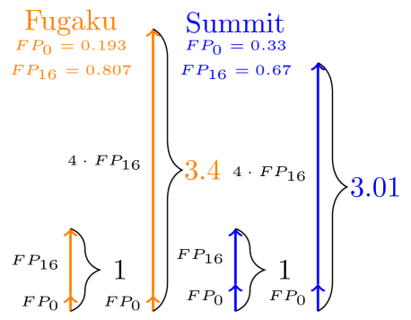
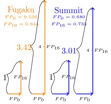
Figure 9: Left: The serial summing of payload and non-payload contributions (assumes no parallelization and/or no blocking. Right: The parallel summing of payload and non-payload contributions (assumes parallelization and enables to consider mutual blocking)

Table 1 shows the data calculated from the published values in the TOP500 list for supercomputers $Fugaku$ and $Summit$, together with their parameters calculated as described above, using the time-aware summing model. There is no significant difference between the values derived using the two models in the discussed simple workload case. The values in the figures are given in units of payload performance ratios; the values in the table are given in units of the respective $\alpha$ contributions. We can compare the numbers only as discussed below.

The values $Eff_{64}$ and $Eff_{16}$ are calculated from the corresponding published $R_{Max}/R_{Peak}$ values. We calculate Amdahl’s parameter using Eq. (5) for the two different operand lengths. As discussed, $(1-\alpha)$ is the sequential portion of the total measurement time (aka non-payload to payload ratio). Assuming that the time unit is the total measurement time, the limiting time of performing a floating operation with 64-bit operands $Time_{64}$ (on our arbitrary time scale) is directly derived from the $(1-\alpha_{64})$ value. To get a $Time_{16}$ value on the same scale, we must correct the measured $(1-\alpha_{16})$ values for their differing measurement times (the measured performance ratios 3.42 and 3.01, respectively).

Table 1: Floating point characteristics of supercomputers $Fugaku$ and $Summit$

Name	$Eff_{64}$	$Eff_{16}$	$(1-\alpha_{64})$	$(1-\alpha_{16})$	$Time_{64}$	$Time_{16}$	$F_{16}$	$F_{0}$
Fugaku	0.808	0.691	3.25e-8	6.12e-8	3.25e-8	1.79e-8	0.49e-8	1.3e-8
Summit	0.74	0.557	14.7e-8	33.2e-8	14.7e-8	11.0e-8	1.23e-8	9.77e-8

One cannot compare the absolute values of the data in the last two columns of the table directly with those of the other supercomputer (their measurement time was different). Given that the task and the computing model were the same, we can directly compare the ratios of values $F_{16}$ and $F_{0}$. The proportions of both $F_{0}$ values and $F_{16}/F_{0}$ values show that housekeeping is much better for $Fugaku$ than for $Summit$. Given that their architectures are globally similar, the plausible reason for the difference in their efficacy (and performance) is that in the case of $Summit$, the processor core is in a role of proxy (and in this way it represents a bottleneck), while $Fugaku$ uses ”assistant cores”. The housekeeping increases latency and significantly decreases the performance of the system. The plausible reason for $Fugagu$s better $F_{16}$ values is the clever use (and positioning! see VeghTemporal:2020 ) of L2-level cache memories.

In the case of $Summit$, we also know its HPCG efficiency. In its case the $Time_{64}^{HPCG}$ value is $2.08\cdot e-5$, i.e. several hundred times higher than $Time_{64}^{HPL}$. Given that $F_{16}$ and $F_{64}$ are the same in the case of the two benchmarks, the difference is caused by $F_{0}$. In the long run, the different workload (iteration, more intensive communication, ”sparse” computation forcing different cache utilization) forces different $F_{0}$ value, and that leads to ”different efficiencies” DifferentBenchmarks:2017 of supercomputers under different workloads. Given that we used a single ”snapshot” of measurement times, these values are average values taken for all floating operations instead of actual operating times.

$Fugaku$ used only a fraction of its cores in the benchmark HPCG, so we can validate only the achieved payload performance (but not its efficiency). It is very plausible that HPCG performance reached its roofline, and –because of the higher number of cores– its real HPCG efficiency would be around that of $Taihulight$. Anyhow, it would not be fair either to assume that speculation or to accept their value measured at a different number of cores. There is no measured data.

These data directly underpin that technology is (almost) perfect: contribution from the benchmark calculation HPCG-FP64 is by orders of magnitude larger than the contribution from all the rests. Recalling that the benchmark program imitates the behavior (as defined by the resulting $\alpha$) of real-life programs, one can see that the contribution from other computing-related actors is about a thousand times smaller than the contribution of the computation+communication.

The unique role of ”mixed precision” efficiencies (the third kind of efficiencies of a supercomputer), see the red ’x’ marks in Fig. 6, deserves special attention. Strictly speaking, we cannot correctly position the points in the figure; they belong to a different scale (they are measured on a different HW). On the one side, the same number of operations are performed, using the same amount of PU s. On the other side, four times fewer data are transferred and manipulated. The nominal performance is expected to be four times higher than in the case of using double-precision operands. Without correcting for the more than three times shorter measurement (see below), the efficiency mark is slightly above the corresponding value measured with double length operands (the relative weight of $F_{0}$ is higher); with correction, it is somewhat below it. This difference, however, is noticeable only with benchmark HPL; in the case of HPCG workload, computation (including operand length) has a marginal effect. In the former case, contributions of computation and communication are in the same range of magnitude, competing for dominating the system’s performance. In the latter case, communication dominates performance; computing has a marginal role. This difference is the reason why no data are available for the HPCG benchmark using half-precision operands.

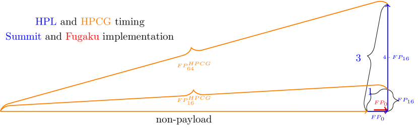
Figure 10: The role of non-payload contribution in defining $HPL$ and $HPCG$ efficiencies, for double and half precision floating operation modes. For visibility, a hypothetic efficiency ratio $E_{HPL}/E_{HPCG}$=10 assumed. The housekeeping (including transfer time and cache misses) dominates, the length of operands has only marginal importance.

Fig. 10 illustrates the role of non-payload performance with respect to operand length. In the figure (for visibility), a hypothetic ratio 10 of efficiencies measured by benchmarks $HPL$ and $HPCG$ was assumed. The non-payload contribution blocks the operation of the floating-point unit. The dominating role of non-payload contribution also means that it is of little importance if we use double or half-precision operands in the computation. The blue vectors essentially represent the case of $Summit$, the red vector represents the $FP_{0}$ value of $Fugaku$ (transformed to scaling of $Summit$). We attribute the difference between their $HPL$ performances to their different $FP_{0}$ values. This difference, however, gets marginal as the workload approaches real-life conditions.

4.6 Further efficiency values

The performance corresponding to $\alpha_{HPL}^{FP0}$ is slightly above 1 EFlops (when making no floating operations, i.e., rather Eops). Another peak performance reported when running genomics code on Summit (by using a mixture of numerical precisions and mostly non-floating point instructions) is 1.88 Eops, corresponding to $\alpha_{Genom}^{FP0}=1*10^{-8}$. Those two values refer to a different mixture of instructions, so the agreement is more than satisfactory.

Our simple calculations result in, that in the case of the benchmark HPL, $FP_{0}$ values are in the order of $FP_{16}$, and that the benchmark HPL is computing bound: reducing housekeeping (including communication) has some sense for ”racing supercomputers”, for real-life applications it has only marginal effect. On the other side, increasing the housekeeping (more communication such as in the case of benchmark HPCG or ANN s) degrades the apparent performance. At a sufficiently large amount of communication VeghScalingANN:2021 , the housekeeping dominates the performance, and the contribution of $FP_{X}$ becomes marginal. For large ANN applications, using $FP_{16}$ operands makes no real difference, their workload defines their performance (and efficiency). The ”commodity supercomputers” can achieve the same payload performance, although they have a much lower number of PU s: The ”racing supercomputers” either cannot use their impressively vast number of cores at all, or using all their cores does not increase their payload performance in solving real-life tasks.

4.7 The effect of clock period’s length

The behavior of time in computing systems is in parallel with the quantal nature of energy, known from modern science. Time in computing systems passes in discrete steps rather than continuously. This difference is not noticeable under usual conditions: both human perception and macroscopic computing operations are a million-fold longer. Under the extreme conditions represented by many-many core systems, however, the quantal nature is the source of the inherent limitation of parallelized sequential systems. The fundamental issue is that operations must be synchronized; asynchronous operation provides performance advantages IBMAsynchronousAPI2017 .

The need to synchronize operations (including those of many-many processors) using a central clock signal is especially disadvantageous when attempting to imitate the behavior of biological systems without such a central signal. Although the intention to provide asynchronous operating mode was a major design point SpiNNaker:2013 , the hidden synchronization (mainly introduced by thinking in conventional SW solutions) led to very poor efficiency NeuralNetworkPerformance:2018 , when the system attempted to perform its flagship goal: simulating the functionality of (a large part of) the human brain.

As we discussed in section 4.1, the performance also depends on the length of measurement time, because of fixed-time contributions. When making only 10 seconds long measurements, the smaller denominator (compared to HPL benchmarking time) may result in up to $10^{3}$ times worse $(1-\alpha_{eff})$ and performance gain values. The dominant limiting factor, however, is a different one.

In brain simulation, a $1~{}ms$ integration time (essentially, a sampling time) is commonly used NeuralNetworkPerformance:2018 . The biological time (when events happen) and the computing time (how much computing time is required to perform computing operations to describe the same) are not only different but also not directly related. Working with ”signals from the future” must be excluded. For this goal, at the end of this period, one must communicate the calculated new values of the state variables to all (interested) fellow neurons. This action essentially introduces a ”biology clock signal period” million-fold longer than the electronic clock signal period. Correspondingly, the achievable performance is desperately low: the system can simulate less than $10^{5}$ neurons, out of the planned $10^{9}$  NeuralNetworkPerformance:2018 . For a detailed discussion see VeghBrainAmdahl:2019 ; VeghTemporal:2020 ; VeghScalingANN:2021 .

The researchers also investigated NeuralNetworkPerformance:2018 their power consumption efficiency. We presumed that –to avoid obsolete energy consumption– they performed the measurement at the point where involving more cores increases the power consumption but does not increase the payload simulation performance. This assumption resulted in the ”reasoned guess” for the efficiency of brain simulation in Figures 2 and 3. Given that using AI workload (for a discussion from this point of view see VeghScalingANN:2021 ) on supercomputers is of growing importance, the performance gain of a processor-based AI application can be estimated to be between those of HPCG and brain simulation, closer to that of HPCG. As discussed experimentally in DeepNeuralNetworkTraining:2016 and theoretically in VeghScalingANN:2021 , in the case of neural networks (especially in the case of selecting improper layering depth) the efficiency can be much lower than that estimated value.

Recall that since AI nodes usually perform simple calculations compared to the functionality of supercomputer benchmarks, their communication/calculation ratio is much higher, making the efficacy even worse. The experimental research DeepNeuralNetworkTraining:2016 underpins our conclusions :

• ”strong scaling is stalling after only a few dozen nodes”

• ”The scalability stalls when the compute times drop below the communication times, leaving compute units idle. Hence becoming an communication bound problem.”

• ”network layout has a large impact on the crucial communication/compute ratio: shallow networks with many neurons per layer …scale worse than deep networks with less neurons.”

The massively ”bursty” nature of data (different nodes of the layer want to use the communication subsystem simultaneously) also makes the case harder. The commonly used global bus is overloaded with messages (for a detailed discussion see VeghTemporal:2020 ). That overload may lead to a ”communicational collapse” (demonstrated in Figure 5.(a) in  CommunicationCollapse:2018 ): at an extremely large number of cores, exceeding the critical threshold of communication intensity, leads to an unexpected and drastic change of network latency.

5 Accuracy and reliability of our model

As the value of parameters of our model are inferred from non-dedicated single-shot measurements, their reliability is limited. One can verify, however, how our model predicts values derived from later measurements. Supercomputers usually do not have a long lifespan and several documented stages. One of the rare exceptions is supercomputer Piz Daint, and its documented lifetime spans over six years. Different amounts of cores, without and with acceleration, using various accelerators, were used at that period.

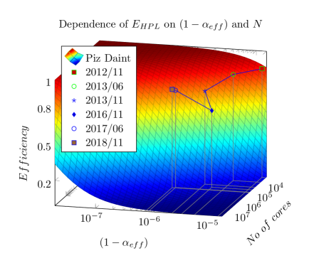
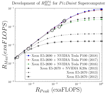
Figure 11: History of supercomputer Piz Daint in terms of efficiency and payload performance TOP500 . The left subfigure shows how the efficiency changed as developers proceeded towards higher performance. The right subfigure shows the reported performance data (the bubbles), together with diagram line calculated from the value as described above. Compare the value of diagram line to measured performance data in the next reported stage.

Figure 11 depicts the performance and efficiency values published during its lifetime, together with diagram lines predicting (at the time of making the prediction) values at higher nominal performance values. The left subfigure shows how changes made in the configuration affected its efficiency (the timeline starts in the top right corner, and a line connects adjacent stages).

In the right subfigure, bubbles represent data published in adjacent editions of the TOP500 lists, the diagram lines crossing them are predictions made from that snapshot. We shall compare the predicted value to the value published in the next list. It is especially remarkable that introducing GPGPU acceleration resulted only in a slight increase (in good agreement with Lee:GPUvsCPU2010 and WhyNotExascale:2014 ) compared to the value expected based purely on the increase in the number of cores. Although between our ”samplings”, more than one parameter changed, that is, the net effect cannot be demonstrated clearly, the measured data sufficiently underpin our limited validity conclusions and show that theory correctly describes the tendency of development of performance and efficiency, and even its predicted performance values are reasonably accurate.

Introducing GPU accelerator is a one-time performance increasing step WhyNotExascale:2014 , and the theory cannot take it into account. Notice that introducing an accelerator increased the payload performance but decreased efficiency (copying data from one address space to another increases latency). Changing the accelerator to another type with slightly higher performance (but higher latency due to its larger GPGPU memory) caused a slight decrease in the absolute performance because of the considerably dropped efficiency.

6 Towards zettaflops

As detailed above, our theoretical model enables us to calculate the payload performance in first-order approximation at any nominal performance value. In the light of all of this, one can estimate a short time and a long term development of supercomputer performance, see Figs. 12.A and 12.B. We calculated the diagram lines using Eq. (4), with $\alpha$ parameter values derived from TOP500 data of Summit supercomputer; the bubbles show measured values. The diagram lines from the bottom up show the double floating precision HPCG, HPL and the half precision MixedPrecisionHPL:2018 HPL (HPL-AI) diagrams. Given that we calculated our parameter values from a snapshot and that the calculation is essentially an extrapolation, furthermore that at high nominal performance values using the second-order approximation is more and more pressing, the predictions shown in Figure 12 are rough and very optimistic approximations. However, they show values somewhat similar to actual upper limiting values.

In addition to the measured and published performance data, two more diagram lines representing two more calculated $\alpha$ values are also depicted. The ’FP0’ (orange) diagram line is calculated with the assumption that the supercomputer makes the stuff needed to perform the HPL benchmark, but actual FP operations are not performed. In other words, the computer works with zero-bit length floating operands (FP0).

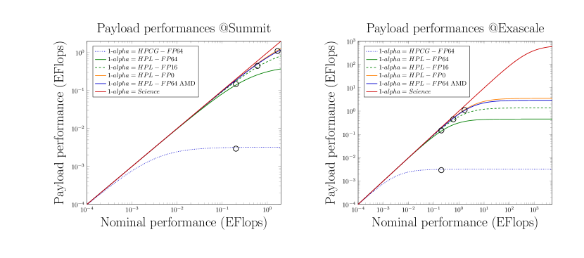
Figure 12: The tendency of development of payload performance in the near and farther future of supercomputing. The parameters of $Summit$ are used for illustration, and for comparison, the double-precision performance diagram line of $Frontier$ is also displayed. The diagram lines are calculated from the theory, the marks are the measured values from the database TOP500 TOP500 and MixedPrecisionHPL:2018 .

The ’Science’ (red) diagram line is calculated with the assumption that nothing is calculated, but science (the finite propagation time due to the limited speed of light) limits the payload performance. The nonlinearity of the payload performance around the Eflops nominal performance is visible and depends on the amount of computing+communication and nominal performance (represented by the number of cores).

Figure 12B shows the farther future (in first-order approximation): towards Zflops ChinaExascale:2018 . No surprise that all payload performance diagram lines run into saturation, even the ’FP0’ and ’Science’ ones. For comparison, double-precision payload performance of $Frontier$ is also displayed: the higher single-processor performance and lower internal latency did not change the general behavior of supercomputing. Recall that the diagram lines are calculated in the first-order approximation. In the second-order approximation, it is expected that diagram lines reach their inflection point and break down. These top supercomputers are near to that point; this is why their development stalled.

7 Analogies with the case of modern vs classic science

The analogies in this section do not want to imply direct correspondence between certain physical and computing phenomena. Instead, we wish to draw the attention to both that under extreme conditions we may encounter qualitatively different behavior, and that scrutinizing certain, formerly unnoticed or neglected aspects enables us to explain the new phenomena. Unlike in nature, in computing, we can change the technical implementation of critical points, and through this, we can alter the behavior of computing systems. For a detailed discussion and more details see VeghModernParadigm:2019 .

7.1 Adding payload performances

Eq. (6) tells that (in first-order approximation) the speedup of a parallelized computing system cannot exceed $1/(1-\alpha)$; a well-known consequence of Amdahl’s statement. Due to this, the computing performance of a system cannot be increased above the performance defined by the single-processor performance, the parallelization technology, and the number of processors. The laws of nature prohibit from exceeding a specific computing performance (using the classical paradigm and its classical implementation). There is an analogy between adding speeds in physics and adding performances in computing. In both cases, a correction term is introduced that provides a noticeable effect only at tremendous values. It seems to be an interesting parallel, that both nature and extremely cutting-edge technical (computing) systems show up some extraordinary behavior, i.e., the linear behavior experienced under normal conditions gets strongly non-linear at large values of the independent variable. That behavior makes the validity of linear extrapolations as well as the linear addition of performances at least questionable at high performance values in computing.

7.2 Quantal nature of computing time

In computing, the cooperation of components needs some kind of synchronization. Typically, it uses a central clock (with clock domains and distribution trees). In today’s technology, the length of the clock cycle is in the $ns$ range, so they seem to be quasi-continuous for the human perception. In some applications, for example, when attempting to imitate the parallel operation of the nervous system, the non-continuous nature of computing time comes to light. In that case, the independently running neurons must be put back to their biological scale, i.e., they stop at the end of the ”integration grid time” values, and distribute their result to the peer neurons. This synchronization introduces a ”biological clock time”, about a million-fold longer than the ”processor clock time”, and limits the achievable parallelization gain. The effect is noticeable only at a vast number of cores. The limit is conceptual but made much worse with the ”communication burst”: the appearance of the simultaneous need for communication in the neural networks represents. For details see VeghBrainAmdahl:2019 .

7.3 ’Quantum states’ of supercomputers

As discussed in VeghModernParadigm:2019 , the behavior of computing systems under extreme conditions shows surprising parallels with the behavior of natural objects. Really, ”More Is Different” MoreIsDifferent1972 . The behavior of supercomputers is somewhat analogous to the behavior of quantum systems, where the measurement selects one of its possible states (and at the same time kills all other possible states). In computing, a supercomputer –as a general-purpose computing system– has the potential of high performance defined by the impressive parameters of its components, for all possible workflows. However, when we run a computation (that is, we measure the computing performance of our computer), that workload selects the best possible combination of limitations that defines its performance for the given workload and kills all other potential performances.

The logical dependence of the operation of the components implicitly also means their temporal dependence VeghTemporal:2020 , and it introduces idle times to computing. In this way, the workload defines how much of those potential abilities can be used: the datasheet values represent hard limits, and their workload sets the soft limits, given that the components block each other’s operation. The workload defines a fill-out factor: it introduces different idle times into component’s operation, and in this way, forces workload-defined soft performance limits to the components of the supercomputer. Different workloads force different limitations (use their available resources differently), giving a natural explanation of their ”different efficiencies” DifferentBenchmarks:2017 . In other words, running some computation destroys the potentially achievable high performance, defined individually by its components.

Benchmarking such computing systems introduces one more limiting component: the needed computation. For floating-point computations, the ’best possible’ (producing the highest figures of merit) benchmark is HPL. With the development of parallelization and processor technology, floating computation itself became the major contributor in defining the system’s efficiency and performance. Since the benchmark measurement method itself is a computation, the best measurable floating payload performance value cannot be smaller than the benchmark procedure itself represents.

For real-life programs (such as HPCG) their workload-defined performance level (saturation value) are already set well below the Eflops nominal performance, see Fig. 2. Further enhancements in technology, such as tensor processors and OpenCAPI connection bus, can slightly increase their saturation level but cannot change the science-defined shape of the diagram line.

8 Conclusion

Supercomputers reached their technical limitations, their development is out of steam. To continue enhancing the components of a supercomputer that wants to run any calculation without changing its underlying computing paradigm is not worth any more. To enter the ”next level”, really renewing the classic computing paradigm is needed RenewingComputingVegh:2018 ; IntroducingEMPA2018 ; VeghSPAEMPA:2020 ; VeghTemporal:2020 .

The ironic remark that ’Perhaps supercomputers should just be required to have written in small letters at the bottom on their shiny cabinets: “Object manipulations in this supercomputer run slower than they appear.” DifferentBenchmarks:2017 ’ is becoming increasingly relevant. The impressive numbers about the performance of their components (including single-processor and/or GPU performance and speed of interconnection) are becoming less relevant when going to the extremes. Given that the most substantial $\alpha$ contribution today takes its origin in the computation the supercomputer runs, even the best possible benchmark HPL dominates floating performance measurement. Enhancing other contributions, such as interconnection, result in marginal enhancement of their payload performance, i.e., the overwhelming majority of expenses increase their ”dark performance” only. Because of this, the answers to the questions in the title are: there are as many performance values as many measurement methods (that vary with how big portion of available cores are used in the measurement), and actually benchmarks measure mainly how much mathematics/communication the benchmark program does, rather than the supercomputer architecture (provided that all components deliver their technically achievable best parameters).

References

- (1) S. H. Fuller and L. I. Millett, The Future of Computing Performance: Game Over or Next Level? National Academies Press, Washington, 2011.
- (2) A. Mehonic and A. Kenyon, “Brain-inspired computing needs a master plan,” Nature, vol. 604, pp. 255–260, 2022.
- (3) G. M. Amdahl, “Validity of the Single Processor Approach to Achieving Large-Scale Computing Capabilities,” in AFIPS Conference Proceedings, vol. 30, 1967, pp. 483–485.
- (4) J. P. Singh, J. L. Hennessy, and A. Gupta, “Scaling parallel programs for multiprocessors: Methodology and examples,” Computer, vol. 26, no. 7, pp. 42–50, 1993.
- (5) J. Végh and A. Tisan, “The need for modern computing paradigm: Science applied to computing,” in Computational Science and Computational Intelligence CSCI The 25th Int’l Conf on Parallel and Distributed Processing Techniques and Applications. IEEE, 2019, pp. 1523–1532. [Online]. Available: http://arxiv.org/abs/1908.02651
- (6) J. Végh, J. Vásárhelyi and D. Drótos, “The performance wall of large parallel computing systems,” in Lecture Notes in Networks and Systems 68. Springer, 2019, pp. 224–237. [Online]. Available: https://link.springer.com/chapter/10.1007%2F978-3-030-12450-2_21
- (7) I. Markov, “Limits on fundamental limits to computation,” Nature, vol. 512(7513), pp. 147–154, 2014.
- (8) Liao, Xiang-ke et al, “Moving from exascale to zettascale computing: challenges and techniques,” Frontiers of Information Technology & Electronic Engineering, vol. 19, no. 10, pp. 1236–1244, 2018. [Online]. Available: https://doi.org/10.1631/FITEE.1800494
- (9) M. Feldman, “Exascale Is Not Your Grandfather’s HPC,” https://www.nextplatform.com/2019/10/22/exascale-is-not-your-grandfathers-hpc/, 2019.
- (10) TOP500, “Top500 list of supercomputers,” https://www.top500.org/lists/top500/ (Accessed on Oct 24, 2021), 2021.
-
(11)
US Government NSA and DOE, “A Report from the NSA-DOE Technical Meeting on
High Performance Computing,” https://www.nitrd.gov/
nitrdgroups/images/b/b4/NSA_DOE_HPC_TechMeetingReport.pdf, 2016. - (12) R. F. Service, “Design for U.S. exascale computer takes shape,” Science, vol. 359, pp. 617–618, 2018.
- (13) European Commission, “Implementation of the Action Plan for the European High-Performance Computing strategy,” http://ec.europa.eu/newsroom/dae/document.cfm? doc_id=15269, 2016.
- (14) Extremtech, “ Japan Tests Silicon for Exascale Computing in 2021.” https://www.extremetech.com/computing/ 272558-japan-tests-silicon-for-exascale-computing -in-2021, 2018.
- (15) K. Bourzac, “Streching supercomputers to the limit,” Nature, vol. 551, pp. 554–556, 2017.
- (16) IEEE Spectrum, “Two Different Top500 Supercomputing Benchmarks Show Two Different Top Supercomputers,” https://spectrum.ieee.org/tech-talk/computing/hardware/two-different-top500-supercomputing- benchmarks-show -two -different-top-supercomputers, 2017.
-
(17)
H. Simon, “Why we need Exascale and why we won’t get there by 2020,”
https://www.researchgate.net/publication/261879110
_Why_we_need_Exascale_and_why_we_won’t_get _there_by_2020 (Accessed on Oct 23, 2021), 2014. - (18) J. L. Gustafson, “Reevaluating Amdahl’s Law,” Commun. ACM, vol. 31, no. 5, pp. 532–533, 1988.
- (19) S. Krishnaprasad, “Uses and Abuses of Amdahl’s Law,” J. Comput. Sci. Coll., vol. 17, no. 2, pp. 288–293, Dec. 2001.
- (20) Y. Shi, “Reevaluating Amdahl’s Law and Gustafson’s Law,” https://www.researchgate.net/publication/ 228367369_Reevaluating_Amdahl’s_law_and _Gustafson’s_law, 1996.
- (21) J. Végh, “Which scaling rule applies to Artificial Neural Networks,” Neural Comput & Applic, 2021. [Online]. Available: http://link.springer.com/article/10.1007/ s00521-021-06456-y
- (22) www.top500.org, “Intel dumps knights hill, future of xeon phi product line uncertain,” https://www.top500.org/news/intel-dumps-knights-hill-future-of-xeon-phi-product-line-uncertain///, 2017.
- (23) C. Liu, G. Bellec, B. Vogginger, D. Kappel, J. Partzsch, F. Neumärker, S. Höppner, W. Maass, S. B. Furber, R. Legenstein, and C. G. Mayr, “Memory-Efficient Deep Learning on a SpiNNaker 2 Prototype,” Frontiers in Neuroscience, vol. 12, p. 840, 2018. [Online]. Available: https://www.frontiersin.org/article/10.3389/fnins.2018.00840
- (24) Top500.org, “Retooled Aurora Supercomputer Will Be America’s First Exascale System,” https://www.top500.org/news/retooled-aurora-supercomputer-will-be -americas- first-exascale-system/, 2017.
- (25) J. Dongarra, “Report on the Fujitsu Fugaku System,” University of Tennessee Department of Electrical Engineering and Computer Science, Tech. Rep. Tech Report ICL-UT-20-06, 2016.
- (26) S. Kunkel, M. Schmidt, J. M. Eppler, H. E. Plesser, G. Masumoto, J. Igarashi, S. Ishii, T. Fukai, A. Morrison, M. Diesmann, and M. Helias, “Spiking network simulation code for petascale computers,” Frontiers in Neuroinformatics, vol. 8, p. 78, 2014.
- (27) S. B. Furber, D. R. Lester, L. A. Plana, J. D. Garside, E. Painkras, S. Temple, and A. D. Brown, “Overview of the SpiNNaker System Architecture,” IEEE Transactions on Computers, vol. 62, no. 12, pp. 2454–2467, 2013.
- (28) S. J. van Albada, A. G. Rowley, J. Senk, M. Hopkins, M. Schmidt, A. B. Stokes, D. R. Lester, M. Diesmann, and S. B. Furber, “Performance Comparison of the Digital Neuromorphic Hardware SpiNNaker and the Neural Network Simulation Software NEST for a Full-Scale Cortical Microcircuit Model,” Frontiers in Neuroscience, vol. 12, p. 291, 2018.
- (29) J. Végh, “How Amdahl’s Law limits performance of large artificial neural networks,” Brain Informatics, vol. 6, pp. 1–11, 2019. [Online]. Available: https://braininformatics.springeropen.com/ articles/10.1186/s40708-019-0097-2
- (30) P. W. Anderson, “More Is Different,” Science, vol. 177, pp. 393–396, 1972.
- (31) J. Végh, “Introducing temporal behavior to computing science,” in Advances in Software Engineering, Education, and e-Learning, H. R. Arabnia, L. Deligiannidis, F. G. Tinetti, and Q.-N. Tran, Eds. Springer International Publishing, 2021, pp. 471–491.
- (32) D. Patterson and J. Hennessy, Eds., Computer Organization and design. RISC-V Edition. Morgan Kaufmann, 2017.
- (33) R. Waser, Ed., Advanced Electronics Materials and Novel Devices, ser. Nanoelectronics and Information Technology. Wiley-VCH, 2012.
- (34) K. Hwang and N. Jotwani, Advanced Computer Architecture: Parallelism, Scalability, Programmability, 3rd ed. Mc Graw Hill, 2016.
- (35) V. Weaver, D. Terpstra, and S. Moore, “Non-determinism and overcount on modern hardware performance counter implementations,” in 2013 IEEE International Symposium on Performance Analysis of Systems and Software (ISPASS) 21-23 April 2013; Austin, TX, USA, 2013, pp. 215–224.
- (36) P. Molnár and J. Végh, “Measuring Performance of Processor Instructions and Operating System Services in Soft Processor Based Systems,” in 18th Internat. Carpathian Control Conf. ICCC, 2017, pp. 381–387.
- (37) F. Ellen, D. Hendler, and N. Shavit, “On the Inherent Sequentiality of Concurrent Objects,” SIAM J. Comput., vol. 43, no. 3, p. 519–536, 2012.
- (38) L. Yavits, A. Morad, and R. Ginosar, “The effect of communication and synchronization on Amdahl’s law in multicore systems,” Parallel Computing, vol. 40, no. 1, pp. 1–16, 2014.
- (39) J. Végh and P. Molnár, “How to measure perfectness of parallelization in hardware/software systems,” in 18th Internat. Carpathian Control Conf. ICCC 28-31 May 2017; Sinaia, Romania, 2017, pp. 394–399.
- (40) F. Zheng, H.-L. Li, H. Lv, F. Guo, X.-H. Xu, and X.-H. Xie, “Cooperative computing techniques for a deeply fused and heterogeneous many-core processor architecture,” Journal of Computer Science and Technology, vol. 30, no. 1, pp. 145–162, 2015.
- (41) M. Mohammadi and T. Bazhirov, “Comparative Benchmarking of Cloud Computing Vendors with High Performance Linpack,” in Proceedings of the 2Nd International Conference on High Performance Compilation, Computing and Communications, Hong Kong, Hong Kong, ser. HP3C. New York, NY, USA: ACM, 2018, pp. 1–5.
- (42) A. H. Karp and H. P. Flatt, “Measuring Parallel Processor Performance,” Commun. ACM, vol. 33, no. 5, pp. 539–543, May 1990.
- (43) S. Williams, A. Waterman, and D. Patterson, “Roofline: An insightful visual performance model for multicore architectures,” Commun. ACM, vol. 52, no. 4, pp. 65–76, 2009.
- (44) G. D’Angelo and S. Rampone, “Towards a HPC-oriented parallel implementation of a learning algorithm for bioinformatics applications,” BMC Bioinformatics, vol. 15, 2014.
- (45) T. Ippen, J. M. Eppler, H. E. Plesser, and M. Diesmann, “Constructing Neuronal Network Models in Massively Parallel Environments,” Frontiers in Neuroinformatics, vol. 11, p. 30, 2017.
- (46) G. Bell, D. H. Bailey, J. Dongarra, A. H. Karp, and K. Walsh, “A look back on 30 years of the Gordon Bell Prize,” The International Journal of High Performance Computing Applications, vol. 31, no. 6, pp. 469–484, 2017. [Online]. Available: https://doi.org/10.1177/1094342017738610
- (47) J. Dongarra, M. A. Heroux, and P. Luszczek, “High-performance conjugate-gradient benchmark: A new metric for ranking high-performance computing systems,” The International Journal of High Performance Computing Applications, 2015. [Online]. Available: https://doi.org/10.1177/1094342015593158
- (48) HPCG Benchmark, “HPCG Benchmark,” http://www.hpcg-benchmark.org/, 2016.
- (49) “Frontier supercomputer debuts as world’s fastest, breaking exascale barrier,” 2022. [Online]. Available: https://www.ornl.gov/news/frontier-supercomputer-debuts-worlds-fastest-breaking-exascale-barrier
- (50) J. Dongarra, “Report on the Sunway TaihuLight System,” University of Tennessee Department of Electrical Engineering and Computer Science, Tech. Rep. Tech Report UT-EECS-16-742, 2016. [Online]. Available: http://www.netlib.org/utk/people/JackDongarra/PAPERS/sunway-report-2016.pdf
- (51) C.-H. Hsu, J. A. Kuehn, and S. W. Poole, “Towards efficient supercomputing: searching for the right efficiency metric,” in Proceedings of the 3rd ACM/SPEC International Conference on Performance Engineering, 2012, p. 1157–162. [Online]. Available: https://doi.org/10.1145/2188286.2188309
- (52) D. S. Martin, “HARDWARE AND SOFTWARE TECHNIQUES FOR SCALABLE THOUSAND-CORE SYSTEMS,” Ph.D. dissertation, Stanford University, Berkeley, 2012.
- (53) “At Long Last, HPC Officially Breaks The Exascale Barrier,” 2022. [Online]. Available: https://www.nextplatform.com/2022/05/30/at-long-last-hpc-officially-breaks-the-exascale-barrier/
- (54) “The AMD “Aldebaran” GPU That Won Exascale,” 2022. [Online]. Available: https://www.nextplatform.com/2021/11/09/the-aldebaran-amd-gpu-that-won-exascale/
- (55) “Limits of Instruction-level Parallelism,” pp. 176–188, apr 1991. [Online]. Available: https://www.hpcwire.com/2022/05/30/top500-exascale-is-officially-here-with-debut-of-frontier/
- (56) “Frontier: Step By Step, Over Decades, To Exascale,” 2022. [Online]. Available: https://www.nextplatform.com/2022/05/30/frontier-step-by-step-over-decades-to-exascale/
- (57) D. Tsafrir, “The context-switch overhead inflicted by hardware interrupts (and the enigma of do-nothing loops),” in Proceedings of the 2007 Workshop on Experimental Computer Science, San Diego, California, ser. ExpCS ’07. New York, NY, USA: ACM, 2007, pp. 3–3.
- (58) F. M. David, J. C. Carlyle, and R. H. Campbell, “Context Switch Overheads for Linux on ARM Platforms,” in Proceedings of the 2007 Workshop on Experimental Computer Science, San Diego, California, ser. ExpCS ’07. New York, NY, USA: ACM, 2007. [Online]. Available: http://doi.acm.org/10.1145/1281700.1281703
- (59) IBM, “Why IBM sees OpenCAPI and OMI as the future for accelerator-driven computing,” https://www.techrepublic.com/article/why-ibm-sees-opencapi-and-omi-as-the-future-for-accelerator-driven-computing/, 2019.
- (60) V. W. Lee, C. Kim, J. Chhugani, M. Deisher, D. Kim, A. D. Nguyen, N. Satish, M. Smelyanskiy, S. Chennupaty, P. Hammarlund, R. Singhal, and P. Dubey, “Debunking the 100X GPU vs. CPU Myth: An Evaluation of Throughput Computing on CPU and GPU,” in Proceedings of the 37th Annual International Symposium on Computer Architecture, ser. ISCA ’10, Saint-Malo, France. New York, NY, USA: ACM, 2010, pp. 451–460. [Online]. Available: http://doi.acm.org/10.1145/1815961.1816021
- (61) S. Moradi and R. Manohar, “The impact of on-chip communication on memory technologies for neuromorphic systems,” Journal of Physics D: Applied Physics, vol. 52, no. 1, p. 014003, oct 2018.
- (62) Y. Ao, C. Yang, F. Liu, W. Yin, L. Jiang, and Q. Sun, “Performance Optimization of the HPCG Benchmark on the Sunway TaihuLight Supercomputer,” ACM Trans. Archit. Code Optim., vol. 15, no. 1, pp. 11:1–11:20, Mar. 2018.
- (63) A. Haidar, S. Tomov, J. Dongarra, and N. J. Higham, “Harnessing GPU Tensor Cores for Fast FP16 Arithmetic to Speed Up Mixed-precision Iterative Refinement Solvers,” in Proceedings of the International Conference for High Performance Computing, Networking, Storage, and Analysis, ser. SC ’18. IEEE Press, 2018, pp. 47:1–47:11.
- (64) P. Gohil, J. Horn, J. He, A. Papageorgiou, and C. Poole, “IBM CICS Asynchronous API: Concurrent Processing Made Simple,” http://www.redbooks.ibm.com/redbooks/pdfs/sg248411.pdf , 2017.
- (65) J. Keuper and F.-J. Pfreundt, “Distributed Training of Deep Neural Networks: Theoretical and Practical Limits of Parallel Scalability,” in 2nd Workshop on Machine Learning in HPC Environments (MLHPC). IEEE, 2016, pp. 1469–1476. [Online]. Available: https://www.researchgate.net/publication/308457837
- (66) J. Végh, Renewing computing paradigms for more efficient parallelization of single-threads, ser. Advances in Parallel Computing. IOS Press, 2018, vol. 29, ch. 13, pp. 305–330. [Online]. Available: https://arxiv.org/abs/1803.04784
- (67) J. Végh, “Introducing the Explicitly Many-Processor Approach,” Parallel Computing, vol. 75, pp. 28 – 40, 2018.
- (68) J. Végh, “How to Extend Single-Processor Approach to Explicitly Many-Processor Approach,” in Advances in Software Engineering, Education, and e-Learning, H. R. Arabnia, L. Deligiannidis, F. G. Tinetti, and Q.-N. Tran, Eds. Springer International Publishing, 2021, pp. 435–458. [Online]. Available: https://arxiv.org/abs/2006.00532