Compact Quasi-Newton Preconditioners for SPD linear systems

Abstract

In this paper preconditioners for the Conjugate Gradient method are studied to solve the Newton system with symmetric positive definite Jacobian. In particular, we define a sequence of preconditioners built by means of SR1 and BFGS low-rank updates. We develop conditions under which the SR1 update maintains the preconditioner SPD. Spectral analysis of the SR1 preconditioned Jacobians shows an improved eigenvalue distribution as the Newton iteration proceeds. A compact matrix formulation of the preconditioner update is developed which reduces the cost of its application and is more suitable for parallel implementation. Some notes on the implementation of the corresponding Inexact Newton method are given and numerical results on a number of model problems illustrate the efficiency of the proposed preconditioners.

1 Introduction

The purpose of this work is to develop efficient preconditioners for the linear systems arising in the Inexact Newton method. The Newton method computes the solution of a system of nonlinear equations $\mbox{\boldmath$F$}(\mbox{\boldmath$x$})=0$, with $\mbox{\boldmath$F$}:\mathbb{R}^{n}\rightarrow\mathbb{R}^{n}$ iteratively by generating a sequence of approximations. Assuming that each component of $F$, $f_{i}$, is differentiable, the Jacobian matrix $J(\mbox{\boldmath$x$})$ is defined by

$$J(\mbox{\boldmath$x$})_{ij}=\frac{\partial f_{i}}{\partial x_{j}}(\mbox{\boldmath$x$}),$$

and the Newton step is written as

$$\left\{\begin{array}[]{ccc}J(\mbox{\boldmath$x$}_{k})\mbox{\boldmath$s$}_{k}&=&-\mbox{\boldmath$F$}(\mbox{\boldmath$x$}_{k})\\ \mbox{\boldmath$x$}_{k+1}&=&\mbox{\boldmath$x$}_{k}+\mbox{\boldmath$s$}_{k}\end{array}\right..$$ (1)

Thus, the method involves the solution of a linear system with the Jacobian matrix. In this work it will be assumed that the Jacobian is a symmetric positive definite (SPD) matrix, as it happens in a number of applications such as, for instance, unconstrained optimization of convex problems, discretization of nonlinear PDEs by e.g. the Picard method [6], or eigensolution of SPD matrices using the (simplified) Jacobi-Davidson method [21, 4, 3]. When $J$ is large and sparse, iterative methods are recommended to solve the linear system with the Jacobian matrix in (1).

The issue of devising preconditioners for the sequences of linear systems arising in the application of an (Inexact) Newton method to nonlinear problems has been addressed e.g. in [17, 18]. To construct a sequence of preconditioners $\{P_{k}\}$ for the Preconditioned Conjugate Gradient (PCG) solution of the Newton systems we use Quasi-Newton approximations of the Jacobian matrix as in [2]. In particular we develop and compare two approaches based on the symmetric Quasi-Newton formulas: SR1 and BFGS. These low-rank corrections have been used as preconditioners in previous papers. We mention, among the others, [19] where the BFGS preconditioner is named balancing preconditioner, [10] where the authors use a single-vector version of the SR1 update, and the work in [16] where both BFGS and SR1 updates are reviewed and used in the framework of iterative eigensolvers. In [1] a bounded deterioration property has been proved for the BFGS preconditioners which implies that $\|I-P_{k}J(\mbox{\boldmath$x$}_{k})\|$ can be made as small as desired depending both on the closeness of $\mbox{\boldmath$x$}_{0}$ to the exact solution and of the initial preconditioner $P_{0}$ to the inverse of the initial Jacobian. BFGS-based sequences of preconditioners have been successfully used in the acceleration of inner iterative solvers in the framework of eigensolution of large and sparse SPD matrices [4].

Differently from the BFGS sequence the SR1 update formula is not expected to provide SPD preconditioners even if the initial one is so. In this work, we will give some some conditions under which it is possible to prove symmetric positive definiteness of the SR1 sequence. Moreover, since in the SR1 case the bounded deterioration property does not generally hold, we will prove that the spectral distribution of the preconditioned matrix at step $k+1$: $P_{k+1}J(\mbox{\boldmath$x$}_{k+1})$ is not worst than that of the preconditioned matrix at step $k$.

Application of this kind of preconditioners requires, in addition to the application of the initial approximation of $J(\mbox{\boldmath$x$}_{0})^{-1}$, a number of scalar products that may considerably slow down the PCG iteration, even if limited memory variants are considered. In view of a parallel implementation, when a high number of processors is employed, large number of scalar products usually reveals a bottleneck of the overall efficiency. To address this problem, we have developed a compact version of the two classes of preconditioners, following the work in [8] where analogous formula are developed in a more general framework, but not in connection with the idea of preconditioning. These matrix versions of the preconditioner updates allow for the use of BLAS-2 kernels for their applications and, at the same time, may reduce considerably the number of communications among processors.

The remainder of the paper is as follows: in Section 2 we review the theoretical properties of the BFGS sequences of preconditioners and we develop a matrix version of the preconditioner update. Section 3 analyzes the condition under which the SR1 sequence is SPD, shows the theoretical properties of the preconditioned matrices and develops a matrix version of the preconditioner update. In Section 4 we present some numerical results which give evidence of the computational gain provided by the compact formulas and of the good behavior of the SR1 update to accelerate the PCG method. In Section 5 we draw some conclusions.

2 BFGS recurrence as a preconditioner

BFGS-type formulas are used in the context of Quasi-Newton methods to approximate the true Jacobian as the iteration progresses. At a given Newton step, let $B_{k}$ be an approximation of the Jacobian matrix $J_{k}$, while $P_{k}$ denotes its inverse, i.e., $P_{k}=B_{k}^{-1}$. By denoting $\mbox{\boldmath$F$}_{k}=\mbox{\boldmath$F$}(\mbox{\boldmath$x$}_{k})$, let us define the vectors $\mbox{\boldmath$y$}_{k}=\mbox{\boldmath$F$}_{k+1}-\mbox{\boldmath$F$}_{k}$, $\mbox{\boldmath$s$}_{k}=\mbox{\boldmath$x$}_{k+1}-\mbox{\boldmath$x$}_{k}$. The BFGS formula is derived by imposing the following conditions on the inverse Jacobian matrix:

• $P_{k+1}$ must be symmetric and positive definite.

• It must satisfy the secant condition, $P_{k+1}\mbox{\boldmath$y$}_{k}=\mbox{\boldmath$s$}_{k}$.

• Closeness condition: among all the symmetric matrices satisfying the secant equation, $P_{k+1}$ must be the closest matrix to $P_{k}$. Using Frobenius norm:

  $$P_{k+1}=\min_{P}\|P-P_{k}\|$$ (2)

  $$\mbox{subject to}\ \ P=P^{T},\ \ P\mbox{\boldmath$y$}_{k}=\mbox{\boldmath$s$}_{k}.$$

The unique solution to (2) is (see [20])

$$P_{k+1}=V_{k}^{T}P_{k}V_{k}+\rho_{k}\mbox{\boldmath$s$}_{k}\mbox{\boldmath$s$}_{k}^{T}\ ,$$ (3)

where

$$V_{k}=\left(I-\rho_{k}\mbox{\boldmath$y$}_{k}\mbox{\boldmath$s$}_{k}^{T}\right)\ ,\ \rho_{k}=1/\mbox{\boldmath$y$}_{k}^{T}\mbox{\boldmath$s$}_{k}.$$ (4)

By applying the Sherman-Morrison-Woodbury formula to (3) an update formula for the Jacobian matrix approximation $B_{k}$ is obtained as

$$B_{k+1}=B_{k}-\dfrac{B_{k}\mbox{\boldmath$s$}_{k}\mbox{\boldmath$s$}_{k}^{T}B_{k}}{\mbox{\boldmath$s$}_{k}^{T}B_{k}\mbox{\boldmath$s$}_{k}}+\dfrac{\mbox{\boldmath$y$}_{k}\mbox{\boldmath$y$}_{k}^{T}}{\mbox{\boldmath$y$}_{k}^{T}\mbox{\boldmath$s$}_{k}}\ .$$ (5)

Moreover, in order to compute the approximate Jacobian efficiently, especially when the number of non-linear iterations is large, limited-memory Quasi-Newton methods where introduced. L-BFGS methods store only a few pairs of vectors $\{\mbox{\boldmath$s$}_{i},\mbox{\boldmath$y$}_{i}\}$ instead of all vectors generated during the iteration process, i.e., early iteration pairs are discarded. Therefore, the computational and memory storage requirements at each Newton iteration are reduced. This may be helpful for solving large-scale nonlinear problems. More precisely, from equations (3) and (4) we can see that the matrix $P_{k+1}$ is obtained by updating the $P_{k}$ with the pair $\{\mbox{\boldmath$s$}_{k},\mbox{\boldmath$y$}_{k}\}$. After the new iterate is computed, the oldest vector pair in the set is deleted and replaced by the new pair. Thus, the set of vector pairs includes information from the $k_{\max}$ most recent iterations. Moreover if $(k\mod k_{\max})=0$, a new initial preconditioner is computed as $P_{0}\equiv P_{k}$. Starting with an initial matrix $P_{0}$, formula (3) can be written as

$$P_{k} = \left(V_{k-1}^{T}\ldots V_{k-k_{\max}}^{T}\right)P_{0}\left(V_{k-k_{\max}}\ldots V_{k-1}\right)$$ (6)

$$+ \rho_{k-k_{\max}}\left(V_{k-1}^{T}\ldots V_{k-k_{\max}+1}^{T}\right)\mbox{\boldmath$s$}_{k-k_{\max}}\mbox{\boldmath$s$}_{k-k_{\max}}^{T}\left(V_{k-k_{\max}+1}\ldots V_{k-1}\right)$$

$$+ \rho_{k-k_{\max}+1}\left(V_{k-1}^{T}\ldots V_{k-k_{\max}+2}^{T}\right)\mbox{\boldmath$s$}_{k-k_{\max}+1}\mbox{\boldmath$s$}_{k-k_{\max}+1}^{T}\left(V_{k-k_{\max}+2}\ldots V_{k-1}\right)$$

$$\vdots$$

$$+ \rho_{k-1}\mbox{\boldmath$s$}_{k-1}\mbox{\boldmath$s$}_{k-1}^{T}\ .$$

From this expression, the computation of the product $\hat{}\mbox{\boldmath$r$}=P_{k}\mbox{\boldmath$r$}$ for a given residual vector $r$ can be done recursively by performing a sequence of inner products and vector summations involving $\mbox{\boldmath$F$}_{k}$ and the pairs $\{\mbox{\boldmath$s$}_{i},\mbox{\boldmath$y$}_{i}\}$, $i=k-k_{\max},\ldots,k-1$, see Algorithm 1. The computational cost is (at most) $2k_{\max}$ daxpys and $2k_{\max}$ dot products.

for $i=k-1,\ldots,k-k_{\max}$ do

   $\alpha_{i}=\rho_{i}\mbox{\boldmath$s$}_{i}^{T}\mbox{\boldmath$r$}$

   $\mbox{\boldmath$r$}:=\mbox{\boldmath$r$}-\alpha_{i}\mbox{\boldmath$y$}_{i}$

end for

$\hat{}\mbox{\boldmath$r$}=P_{0}\mbox{\boldmath$r$}$

for $i=k-k_{\max},\ldots,k-1$ do

   $\beta=\rho_{i}\mbox{\boldmath$y$}_{i}^{T}\hat{}\mbox{\boldmath$r$}$

   $\hat{}\mbox{\boldmath$r$}:=\hat{}\mbox{\boldmath$r$}+(\alpha_{i}-\beta)\mbox{\boldmath$s$}_{i}$

end for

Algorithm 1 L-BFGS two-loop recursion to compute $\hat{}\mbox{\boldmath$r$}=P_{k}\mbox{\boldmath$r$}$

The implementation of the Inexact-Newton method [9] requires the definition of a stopping criterion for the linear solver (1) based on the nonlinear residual. Thus, the linear iteration is stopped with the test

$$\|J(\mbox{\boldmath$x$}_{k})\mbox{\boldmath$s$}_{k}+F(\mbox{\boldmath$x$}_{k})\|\leq\eta_{k}\|F(\mbox{\boldmath$x$}_{k})\|\ .$$ (7)

The sequence $\{\eta_{k}\}$ will be chosen such that $\eta_{k}=O(\|\mbox{\boldmath$F$}(\mbox{\boldmath$x$}_{k})\|)$. This will guarantee quadratic convergence of the Inexact Newton method and as a consequence, the following result.

Proposition 2.1.

Define $\mbox{\boldmath$e$}_{k}=\mbox{\boldmath$x$}_{\ast}-\mbox{\boldmath$x$}_{k}$. There exist $\delta>0$ and $0<r<1$ such that if $\|\mbox{\boldmath$e$}_{0}\|<\delta$ then $\|\mbox{\boldmath$e$}_{k+1}\|\leq r\|\mbox{\boldmath$e$}_{k}\|$ for every $k$.

If the Jacobian matrices are SPD and so is $P_{0}$, then $P_{k}$ is also SPD under the condition $\mbox{\boldmath$s$}_{k}^{T}\mbox{\boldmath$y$}_{k}>0$ (see Lemma 4.1.1 in [15]). Let $\mbox{\boldmath$e$}_{0}=\mbox{\boldmath$x$}_{*}-\mbox{\boldmath$x$}_{0}$, $E_{k}=J_{k}^{-1}-P_{k}$. The next result establishes that $\|I-P_{k}J(\mbox{\boldmath$x$}_{k})\|$ can be made arbitrarily small by suitable choices of the initial guess $\mbox{\boldmath$x$}_{0}$ and the initial preconditioner $P_{0}$.

Theorem 2.2 (Theorem 3.6 in [1]).

For a fixed $\varepsilon_{1}>0$, there are $\delta_{0}$, $\delta_{B}$ such that if $\|\mbox{\boldmath$e$}_{0}\|<\delta_{0}$ and $\|E_{0}\|<\delta_{B}$ then

$$\|I-P_{k}J_{k}\|<\varepsilon_{1}.$$

2.1 Compact inverse representation of the BFGS update formula

Following [7, 20] we write a compact formula for the direct update

$$B_{k}=B_{0}-\begin{bmatrix}B_{0}S_{k}&Y_{k}\end{bmatrix}\begin{bmatrix}S_{k}^{T}B_{0}S_{k}&L_{k}\\ L_{k}^{T}&-D_{k}\end{bmatrix}^{-1}\begin{bmatrix}S_{k}^{T}B_{0}\\ Y_{k}^{T}\end{bmatrix}$$ (8)

where

$$S_{k}=\begin{bmatrix}\mbox{\boldmath$s$}_{0},&\ldots,&\mbox{\boldmath$s$}_{k-1}\end{bmatrix},\qquad Y_{k}=\begin{bmatrix}\mbox{\boldmath$y$}_{0},&\ldots,&\mbox{\boldmath$y$}_{k-1}\end{bmatrix}$$

and

$$(L_{k})_{(i,j)}=\begin{cases}\mbox{\boldmath$s$}_{i-1}^{T}\mbox{\boldmath$y$}_{j-1}&\text{if}\ i>j,\\ 0&\text{otherwise}\end{cases},\qquad D_{k}=\text{diag}\begin{bmatrix}\mbox{\boldmath$s$}_{0}^{T}\mbox{\boldmath$y$}_{0},&\ldots,&\mbox{\boldmath$s$}_{k-1}^{T}\mbox{\boldmath$y$}_{k-1}\end{bmatrix}.$$

By applying the Sherman-Woodbury-Morrison formula to (8) one obtains an explicit formula for the inverse of $B_{k}$, i.e., $P_{k}$. We have

$$P_{k} = P_{0}-\begin{bmatrix}S_{k}&Z_{k}\end{bmatrix}\begin{bmatrix}R_{k}^{-T}H_{k}R_{k}^{-1}&-R_{k}^{-T}\\ -R_{k}^{-1}&0\end{bmatrix}\begin{bmatrix}S_{k}^{T}\\ Z_{k}^{T}\end{bmatrix},$$

where $S_{k},Y_{k}$ are as before and

$$Z_{k}=P_{0}Y_{k},\qquad(R_{k})_{i,j}=\begin{cases}\mbox{\boldmath$s$}_{i-1}^{T}\mbox{\boldmath$y$}_{j-1}&\text{if}\ i\leq j,\\ 0&\text{otherwise}\end{cases},\qquad H_{k}=D_{k}+Y_{k}^{T}P_{0}Y_{k}.$$ (9)

2.2 Computation of $\hat{}\mbox{\boldmath$r$}=P_{k}\mbox{\boldmath$r$}$

At step $k$, previously to the PCG solution of the $k$-th Newton system, we have to compute $\mbox{\boldmath$z$}_{k-1}=P_{0}\mbox{\boldmath$y$}_{k-1}$ by solving the linear system $B_{0}\mbox{\boldmath$z$}_{k-1}=\mbox{\boldmath$y$}_{k-1}$. Then we have to form recursively

$$S_{k}=\begin{bmatrix}S_{k-1}\ \mbox{\boldmath$s$}_{k-1}\end{bmatrix},\quad Z_{k}=\begin{bmatrix}Z_{k-1}\ \mbox{\boldmath$z$}_{k-1}\end{bmatrix},$$

$$R_{k}=\begin{bmatrix}R_{k-1}&S_{k-1}^{T}\mbox{\boldmath$y$}_{k-1}\\ 0&\mbox{\boldmath$s$}_{k-1}^{T}\mbox{\boldmath$y$}_{k-1}\end{bmatrix},\quad H_{k}=\begin{bmatrix}H_{k-1}&Z_{k-1}^{T}\mbox{\boldmath$y$}_{k-1}\\ \mbox{\boldmath$y$}_{k-1}^{T}Z_{k-1}&(s_{k-1}+\mbox{\boldmath$z$}_{k-1})^{T}\mbox{\boldmath$y$}_{k-1}\end{bmatrix}.$$

During the PCG solver, application of $P_{k}$ to the residual vector takes the steps indicated in Algorithm 2.

1. Solve $B_{0}\hat{\mbox{\boldmath$r$}}=\mbox{\boldmath$r$}$;

2. $\mbox{\boldmath$w$}_{1}=S_{k}^{T}\mbox{\boldmath$r$}$;

3. $\mbox{\boldmath$w$}_{2}=Z_{k}^{T}\mbox{\boldmath$r$}$;

4. Solve $R_{k}\mbox{\boldmath$q$}_{2}=\mbox{\boldmath$w$}_{1};$

5. Solve $R_{k}^{T}\mbox{\boldmath$q$}_{1}=\mbox{\boldmath$w$}_{2}-H_{k}\mbox{\boldmath$q$}_{2}$;

5. $\hat{\mbox{\boldmath$r$}}=\hat{\mbox{\boldmath$r$}}-S_{k}\mbox{\boldmath$q$}_{1}-Z_{k}\mbox{\boldmath$q$}_{2}$.

Algorithm 2 Computation of $\hat{}\mbox{\boldmath$r$}=P_{k}\mbox{\boldmath$r$}$ with compact (L-)BFGS

2.3 Limited memory implementation L-BFGS

If $k>k_{\max}$ then the update of matrices $S_{k},Z_{k},U_{k}$ and $H_{k}$ changes as follows (in MATLAB notation). First, rewrite the matrices by shifting elements corresponding to the last $k_{\max}-1$ updates:

$$S_{k-1} \leftarrow S_{k-1}(:,2:k_{\max})$$

$$Z_{k-1} \leftarrow Z_{k-1}(:,2:k_{\max})$$

$$R_{k-1} \leftarrow R_{k-1}(2:k_{\max},2:k_{\max})$$

$$H_{k-1} \leftarrow H_{k-1}(2:k_{\max},2:k_{\max}).$$

Then, update the matrices with the new entries,

$$S_{k}=\begin{bmatrix}S_{k-1}\ \mbox{\boldmath$s$}_{k-1}\end{bmatrix},\quad Z_{k}=\begin{bmatrix}Z_{k-1}\ \mbox{\boldmath$z$}_{k-1}\end{bmatrix},$$

$$R_{k}=\begin{bmatrix}R_{k-1}&S_{k-1}^{T}\mbox{\boldmath$y$}_{k-1}\\ 0&\mbox{\boldmath$s$}_{k-1}^{T}\mbox{\boldmath$y$}_{k-1}\end{bmatrix},\quad H_{k}=\begin{bmatrix}H_{k-1}&Z_{k-1}^{T}\mbox{\boldmath$y$}_{k-1}\\ \mbox{\boldmath$y$}_{k-1}^{T}Z_{k-1}&(s_{k-1}+\mbox{\boldmath$z$}_{k-1})^{T}\mbox{\boldmath$y$}_{k-1}\end{bmatrix}.$$

3 Preconditioner based on SR1 recurrence

In the L-BFGS updating formula, the matrix $B_{k+1}$ (or $P_{k+1}$) differs from its predecessor $B_{k}$ (or $P_{k}$) by a rank$-2$ matrix. There is a simpler rank$-1$ update that maintains symmetry of the matrix and allows it to satisfy the secant equation. But unlike the rank-2 formulas, this symmetric-rank-1 update, also called SR1, does not guarantee that the updated matrix maintains positive definiteness. The direct SR1 update formula is given by (see [20])

$$B_{k+1}=B_{k}+\dfrac{(\mbox{\boldmath$y$}_{k}-B_{k}\mbox{\boldmath$s$}_{k})(\mbox{\boldmath$y$}_{k}-B_{k}\mbox{\boldmath$s$}_{k})^{T}}{(\mbox{\boldmath$y$}_{k}-B_{k}\mbox{\boldmath$s$}_{k})^{T}\mbox{\boldmath$s$}_{k}}\ .$$ (10)

By applying the Sherman-Morrison formula, one can obtain the corresponding update formula for the preconditioner (we will omit subscript _k in vectors $s$ and $y$ from now on)

$$P_{k+1}=P_{k}+\frac{(\mbox{\boldmath$s$}-P_{k}\mbox{\boldmath$y$})(\mbox{\boldmath$s$}-P_{k}\mbox{\boldmath$y$})^{T}}{\mbox{\boldmath$y$}^{T}(\mbox{\boldmath$s$}-P_{k}\mbox{\boldmath$y$})}$$ (11)

satisfying the secant condition

$$P_{k+1}\mbox{\boldmath$y$}=\mbox{\boldmath$s$}.$$

Formula (11) does not generally provide a sequence of SPD matrices and may not be well defined since the scalar $\mbox{\boldmath$y$}^{T}(\mbox{\boldmath$s$}-P_{k}\mbox{\boldmath$y$})$ can in principle be zero. In the sequel of this Section we will discuss these two issues and we will prove that $P_{k+1}J(\mbox{\boldmath$x$}_{k+1})$ has a more favorable eigenvalue distribution than $P_{k}J(\mbox{\boldmath$x$}_{k})$.

Let us denote with $\Omega$ an open subset of $\mathbb{R}^{n}$, we will make the following standard assumptions on $F$ which we will assume to hold throughout this section.

Standard Assumptions:

1. Equation $\mbox{\boldmath$F$}(\mbox{\boldmath$x$})=0$ has a solution $\mbox{\boldmath$x$}_{*}$.

2. $J(\mbox{\boldmath$x$}):\Omega\to\mathbb{R}^{n\times n}$ is Lipschitz continuous with Lipschitz constant $\gamma$.

3. $J_{*}\equiv J(\mbox{\boldmath$x$}_{*})$ is nonsingular (Set $\alpha=\left\|{J_{*}}^{-1}\right\|$) .

Notation. It is now convenient to indicate with the subscript $c$ every vector or matrix referring to the current iterate and with the subscript $+$ every quantity referring to the new iterate $k+1$. Moreover we will use $J_{+}$ and $J_{c}$ instead of $J(\mbox{\boldmath$x$}_{k+1})$ and $J(\mbox{\boldmath$x$}_{k})$ and $\mbox{\boldmath$F$}_{+},\mbox{\boldmath$F$}_{c}$ instead of $\mbox{\boldmath$F$}(\mbox{\boldmath$x$}_{k+1})$, $\mbox{\boldmath$F$}(\mbox{\boldmath$x$}_{k})$.

Following this notation Newton’s method can be stated as

$$J_{c}\mbox{\boldmath$s$} = -\mbox{\boldmath$F$}_{c}$$

$$\mbox{\boldmath$x$}_{+} = \mbox{\boldmath$x$}_{c}+\mbox{\boldmath$s$}$$

We define the error vectors $\ \mbox{\boldmath$e$}_{+}=\mbox{\boldmath$x$}_{*}-\mbox{\boldmath$x$}_{+},\qquad\mbox{\boldmath$e$}_{c}=\mbox{\boldmath$x$}_{*}-\mbox{\boldmath$x$}_{c}.$

Lemma 1.

Let $\|\mbox{\boldmath$e$}_{c}\|\leq\delta_{0}<\dfrac{1}{\alpha\gamma}$. Then $J_{c}$ is invertible and

$$\|J_{c}^{-1}\|\leq\dfrac{\alpha}{1-\alpha\gamma\delta_{0}}\equiv\alpha_{c}$$

Proof.

Follows from Theorem 1.2.1 in [14], also known as Banach lemma. ∎

The following Lemma will provide relations between the vectors $\mbox{\boldmath$s$},\mbox{\boldmath$y$}$ and $\mbox{\boldmath$e$}_{c}$.

Lemma 2.

There exists $\delta>0$ such that if

$$0<\|\mbox{\boldmath$x$}_{c}-\mbox{\boldmath$x$}_{*}\|\leq\delta\quad$$

then the following relations hold

$$\|\mbox{\boldmath$s$}\|\ \leq 2\|\mbox{\boldmath$e$}_{c}\|$$ (13)

$$y = J_{c}\mbox{\boldmath$s$}+\Delta_{1}\mbox{\boldmath$s$},\qquad\text{with}\quad\|\Delta_{1}\|\leq\gamma\|\mbox{\boldmath$e$}_{c}\|$$ (14)

$$\|\mbox{\boldmath$y$}\| \geq \frac{1-\alpha_{c}\gamma\delta}{\alpha_{c}}\|\mbox{\boldmath$s$}\|\equiv c_{1}\|\mbox{\boldmath$s$}\|$$ (15)

Proof.

From $\mbox{\boldmath$s$}=\mbox{\boldmath$e$}_{c}-\mbox{\boldmath$e$}_{+}$ we have, by Proposition 2.1,

$$\|\mbox{\boldmath$s$}\|\leq\|\mbox{\boldmath$e$}_{+}\|+\|\mbox{\boldmath$e$}_{c}\|\leq(1+r)\|\mbox{\boldmath$e$}_{c}\|\leq 2\|\mbox{\boldmath$e$}_{c}\|.$$

Now from the standard assumptions, and from the fundamental theorem of calculus we have that

$$\mbox{\boldmath$y$}=\mbox{\boldmath$F$}_{+}-\mbox{\boldmath$F$}_{c}=\int_{0}^{1}J(\mbox{\boldmath$x$}_{c}+t\mbox{\boldmath$s$})\mbox{\boldmath$s$}dt=J_{c}\mbox{\boldmath$s$}+\int_{0}^{1}(J(\mbox{\boldmath$x$}_{c}+t\mbox{\boldmath$s$})-J_{c})\mbox{\boldmath$s$}dt=J_{c}\mbox{\boldmath$s$}+\Delta_{1}\mbox{\boldmath$s$},$$ (16)

where $\Delta_{1}=\int_{0}^{1}\left(J(\mbox{\boldmath$x$}_{c}+t\mbox{\boldmath$s$})-J_{c}\right)dt\$. From the standard assumptions, (13) and Proposition 2.1

$$\|\Delta_{1}\|\leq\int_{0}^{1}\|\left(J(\mbox{\boldmath$x$}_{c}+t\mbox{\boldmath$s$})-J_{c}\right)\|dt\leq\int_{0}^{1}\gamma\|\mbox{\boldmath$x$}_{c}+t\mbox{\boldmath$s$}-\mbox{\boldmath$x$}_{c}\|dt=\gamma\int_{0}^{1}t\|\mbox{\boldmath$s$}\|dt\leq\gamma\|\mbox{\boldmath$e$}_{c}\|.$$

Finally from

$$\|J_{c}^{-1}\|\|\mbox{\boldmath$y$}\|\geq\|J_{c}^{-1}\mbox{\boldmath$y$}\|=\|\mbox{\boldmath$s$}+J_{c}^{-1}\Delta_{1}\mbox{\boldmath$s$}\|\geq\|\mbox{\boldmath$s$}\|-\|J_{c}^{-1}\Delta_{1}\mbox{\boldmath$s$}\|\geq\left(1-\alpha_{c}\gamma\|\mbox{\boldmath$e$}_{c}\|\right)\|\mbox{\boldmath$s$}\|$$

if $\delta<\dfrac{1}{\alpha_{c}\gamma}$ then we have

$$\|\mbox{\boldmath$y$}\|\geq\frac{\left(1-\alpha_{c}\gamma\delta\right)\|\mbox{\boldmath$s$}\|}{\alpha_{c}}.$$

∎

3.1 Well definition and positive definiteness of $P_{k+1}$

We now give some evidence that the sequence $\{P_{k}\}$ can be made SPD provided that $P_{0}$ is so. Assume that $P_{c}$ is SPD. Then $P_{+}$ is SPD if the denominator in (11) is positive. Using the results of the previous Lemma we can rewrite the denominator in (11), using $\mbox{\boldmath$s$}=J_{c}^{-1}\mbox{\boldmath$y$}-J_{c}^{-1}\Delta_{1}\mbox{\boldmath$s$}$ from (14), as

$$\mbox{\boldmath$y$}^{T}(\mbox{\boldmath$s$}-P_{c}\mbox{\boldmath$y$})=\mbox{\boldmath$y$}^{T}\mbox{\boldmath$s$}-\mbox{\boldmath$y$}^{T}P_{c}\mbox{\boldmath$y$}=\mbox{\boldmath$y$}^{T}J_{c}^{-1}\mbox{\boldmath$y$}-\mbox{\boldmath$y$}^{T}P_{c}\mbox{\boldmath$y$}-\mbox{\boldmath$y$}^{T}J_{c}^{-1}\Delta_{1}\mbox{\boldmath$s$}.$$

Dividing both sides by $\|\mbox{\boldmath$y$}\|^{2}$ we have that

$$\frac{\mbox{\boldmath$y$}^{T}(\mbox{\boldmath$s$}-P_{c}\mbox{\boldmath$y$})}{\|\mbox{\boldmath$y$}\|^{2}}=\frac{\mbox{\boldmath$y$}^{T}J_{c}^{-1}\mbox{\boldmath$y$}}{\mbox{\boldmath$y$}^{T}\mbox{\boldmath$y$}}-\frac{\mbox{\boldmath$y$}^{T}P_{c}\mbox{\boldmath$y$}}{\mbox{\boldmath$y$}^{T}\mbox{\boldmath$y$}}-\frac{\mbox{\boldmath$y$}^{T}J_{c}^{-1}\Delta_{1}\mbox{\boldmath$s$}}{\mbox{\boldmath$y$}^{T}\mbox{\boldmath$y$}}\geq q_{{J^{-1}_{c}}}(\mbox{\boldmath$y$})-q_{P_{c}}(\mbox{\boldmath$y$})-c_{2}\delta$$ (17)

where $q_{A}(\mbox{\boldmath$y$})$ denotes the Rayleigh quotient for a given SPD matrix $A$ and $c_{2}=\dfrac{\gamma(1+\alpha_{c}\gamma\delta)}{c_{1}^{2}}$ since

$$\left|\frac{\mbox{\boldmath$y$}^{T}J_{c}^{-1}\Delta_{1}\mbox{\boldmath$s$}}{\mbox{\boldmath$y$}^{T}\mbox{\boldmath$y$}}\right|\leq\frac{(1+\alpha_{c}\gamma\delta)(\gamma\delta)\|\mbox{\boldmath$s$}\|^{2}}{c_{1}^{2}\|\mbox{\boldmath$s$}\|^{2}}=\frac{(1+\alpha_{c}\gamma\delta)\gamma}{c_{1}^{2}}\delta=c_{2}\delta.$$

Remark 1.

The expression on the right of (17) is expected to be positive for the following reason. The initial preconditioner $P_{0}$ is usually computed as the inverse of a Cholesky factorization of $A\equiv J(\mbox{\boldmath$x$}_{0})$ i.e. $P_{0}=(LL^{T})^{-1}$. As known this kind of preconditioner is able to capture the largest eigenvalues of the coefficient matrix rather than the lowest ones. As a consequence the typical spectrum of the preconditioned matrices is an interval $[\alpha,\beta]$ with $\alpha$ close to zero and $\beta$ slightly larger than 1. The sign of the eigenvalues of $A^{-1}-(LL^{T})^{-1}=L^{-T}\left(L^{T}A^{-1}L-I\right)L^{-1}$ is related to the sign of those of $L^{T}A^{-1}L-I$ which are therefore larger than $\frac{1}{\beta}-1$. As an example we report the extremal eigenvalues of the preconditioned matrix arising from the FD discretization of the Poisson equation with size $n=39204$ preconditioned with the Cholesky factorizations with either no fill-in or with drop tolerances of $\tau=10^{-3},10^{-5}$.

	$\alpha$	$\beta$
IC(0)	$8.504\times 10^{-4}$	1.2057
$\tau=1e-3$	$2.253\times 10^{-2}$	1.1445
$\tau=1e-5$	$0.5097$	1.0998

In practice, it is rather easy to guarantee that

$$d=\min_{\mbox{\boldmath$y$}\in\mathbb{R}^{n}}q_{A^{-1}}(\mbox{\boldmath$y$})-q_{(LL^{T})^{-1}}(\mbox{\boldmath$y$})=\lambda_{\min}\left(A^{-1}-(LL^{T})^{-1}\right)$$

is bounded away from zero by first roughly estimating $\beta$ and then simply scaling the preconditioner factor $L$ by a scalar to satisfy $\beta<1$.

3.2 Effects of the low-rank update on the eigenvalues of $P_{+}J_{+}$

The following Theorem will state that the SR1 correction is able to set approximately to 1 one eigenvalue of the preconditioned matrix.

Theorem 3.

If $P_{c}$ is SPD and $\delta$ is small enough so that the conclusions of Lemma 2 hold, if moreover the denominator in (11) is positive (with $\|P_{+}\|=\alpha_{1}$), then there is $\delta$ such that if $0<\|\mbox{\boldmath$e$}_{c}\|\leq\delta$ then

$$P_{+}J_{+}\mbox{\boldmath$s$}=\mbox{\boldmath$s$}+\mbox{\boldmath$w$},\qquad\text{with}\quad\|\mbox{\boldmath$w$}\|\leq 6\alpha_{1}\gamma\delta^{2}.$$

Proof.

The secant condition $P_{+}\mbox{\boldmath$y$}=\mbox{\boldmath$s$}$ can be rewritten using (16) as

$$P_{+}(J_{c}\mbox{\boldmath$s$}+\Delta_{1}\mbox{\boldmath$s$})=\mbox{\boldmath$s$}$$

which is equivalent to

$$P_{+}J_{+}\mbox{\boldmath$s$}=\mbox{\boldmath$s$}-P_{+}\Delta_{1}\mbox{\boldmath$s$}+P_{+}(J_{+}-J_{c})\mbox{\boldmath$s$}=\mbox{\boldmath$s$}+\mbox{\boldmath$w$}$$

with

$$\|\mbox{\boldmath$w$}\|\leq\alpha_{1}\gamma\delta\|\mbox{\boldmath$s$}\|+\alpha_{1}\gamma\|\mbox{\boldmath$s$}\|^{2}\leq\ (\text{using }\|\mbox{\boldmath$s$}\|\leq 2\|\mbox{\boldmath$e$}_{c}\|\leq 2\delta)\ \leq 6\alpha_{1}\gamma\delta^{2}.$$

∎

The previous theorem shows that the preconditioned matrix $P_{+}J_{+}$ has an approximate eigenvector $s$ corresponding to the approximate eigenvalue 1, the goodness of the approximation depending on how $\mbox{\boldmath$x$}_{c}$ is close to the exact solution $\mbox{\boldmath$x$}_{*}$. Regarding all other eigenvalues we can observe that $P_{+}J_{+}$ is similar to the SPD matrix $\mbox{$J^{1/2}_{+}$}P_{+}\mbox{$J^{1/2}_{+}$}$ so we denote by $\hat{J}_{+}$ this new matrix and by $\hat{J}_{c}$ its analogous at step $k$, namely $\mbox{$J^{1/2}_{c}$}P_{c}\mbox{$J^{1/2}_{c}$}$. The eigenvalue distribution of $\hat{J}_{+}$ is described by Theorem 5. We will handle the simpler case where $J_{c}$ and $J_{+}$ commute and we premise the following

Lemma 4.

If $J_{c}$ and $J_{+}$ commute and $\delta$ is small enough so that the conclusions of Lemma 2 hold, then

$$\mbox{$\hat{J}_{+}$}=\mbox{$\hat{J}_{c}$}+\mbox{\boldmath$z$}\mbox{\boldmath$z$}^{T}+\Delta_{2}$$ (18)

where

$$z = \frac{\mbox{$J^{1/2}_{c}$}(\mbox{\boldmath$s$}-P_{c}\mbox{\boldmath$y$})}{\sqrt{\mbox{\boldmath$y$}^{T}(\mbox{\boldmath$s$}-P_{c}\mbox{\boldmath$y$})}},\qquad\Delta_{J^{1/2}}=\mbox{$J^{1/2}_{+}$}-\mbox{$J^{1/2}_{c}$}$$ (19)

$$\Delta_{2} = \Delta_{J^{1/2}}P_{+}\Delta_{J^{1/2}}+\Delta_{J^{1/2}}P_{+}+P_{+}\Delta_{J^{1/2}}$$ (20)

$$\|\Delta_{2}\| \leq c_{3}\delta,\quad\text{with}\quad c_{3}=4\alpha_{1}\gamma(1+\sqrt{\alpha_{c}})\delta$$ (21)

Proof.

Multiplying (11) by $J^{1/2}_{+}$ on the left and on the right yields

$$\mbox{$\hat{J}_{+}$}=\mbox{$J^{1/2}_{+}$}P_{c}\mbox{$J^{1/2}_{+}$}+\frac{\mbox{$J^{1/2}_{+}$}(\mbox{\boldmath$s$}-P_{c}\mbox{\boldmath$y$})(\mbox{\boldmath$s$}-P_{c}\mbox{\boldmath$y$})^{T}\mbox{$J^{1/2}_{+}$}}{\mbox{\boldmath$y$}^{T}(\mbox{\boldmath$s$}-P_{c}\mbox{\boldmath$y$})}.$$

Writing $\mbox{$J^{1/2}_{+}$}=\mbox{$J^{1/2}_{c}$}+(\mbox{$J^{1/2}_{+}$}-\mbox{$J^{1/2}_{c}$})$ and substituting at the right hand side yield (18) with definitions (19) and (20). To obtain (21) we develop the following bounds

$$\|J_{+}^{1/2}-J_{c}^{1/2}\| \leq \|J_{+}-J_{c}\|\|\left(J_{+}^{1/2}+J_{c}^{1/2}\right)^{-1}\|\leq 2\gamma\delta\frac{1}{\lambda_{\min}\left(J_{+}^{1/2}+J_{c}^{1/2}\right)}\leq\frac{2\gamma\delta}{\lambda_{\min}(J_{c}^{1/2})}=2\gamma\delta\sqrt{\alpha_{c}}.$$

Hence

$$\|\Delta_{2}\|\leq\alpha_{1}\left(4\gamma^{2}\delta^{2}\alpha_{c}+4\gamma\delta\sqrt{\alpha_{c}}\right)\leq\ (\text{recalling that}\ \delta\gamma\alpha_{c}<1)\ \leq 4\alpha_{1}\gamma(1+\sqrt{\alpha_{c}})\delta\equiv c_{3}\delta.$$

∎

We are able to state the final theorem regarding eigenvalue distribution for $\hat{J}_{+}$, assuming all eigenvalues of $\hat{J}_{+}$ and $\hat{J}_{c}$ are ordered increasingly. Denote furthermore with $\mbox{\boldmath$v$}_{1}$ the eigenvector of $\hat{J}_{c}$ corresponding to $\lambda_{1}(\mbox{$\hat{J}_{c}$})$

Theorem 5.

If $J_{c}$ and $J_{+}$ commute then

$$\lambda_{1}(\mbox{$\hat{J}_{+}$}) \geq\lambda_{1}(\mbox{$\hat{J}_{c}$})+\sqrt{\lambda_{2}(\mbox{$\hat{J}_{c}$})-\lambda_{1}(\mbox{$\hat{J}_{c}$})}\left|\mbox{\boldmath$v$}_{1}^{T}\mbox{\boldmath$z$}\right|-c_{3}\delta$$ (22)

$$\lambda_{k}(\mbox{$\hat{J}_{c}$})-c_{3}\delta\leq \lambda_{k}(\mbox{$\hat{J}_{+}$}) \leq\lambda_{k+1}(\mbox{$\hat{J}_{c}$})+c_{3}\delta,\quad k=2,\ldots,n-1,$$ (23)

$$\lambda_{n}(\mbox{$\hat{J}_{+}$}) \leq\lambda_{n}(\mbox{$\hat{J}_{c}$})+\|\mbox{\boldmath$z$}\|^{2}+c_{3}\delta.$$ (24)

Proof.

Bound (22) comes from Corollary 2.3 in [13]. Bounds (23) and (24) are a direct consequence of Weyl’s theorem [11, Theorem 8.1.8]. ∎

Using the previous theorem we can state a bounded deterioration property regarding the condition number of the preconditioned jacobians:

Corollary 6.

If $J_{c}$ and $J_{+}$ commute and

$$\delta<\frac{\sqrt{\lambda_{2}(\mbox{$\hat{J}_{c}$})-\lambda_{1}(\mbox{$\hat{J}_{c}$})}\left|\mbox{\boldmath$v$}_{1}^{T}\mbox{\boldmath$z$}\right|}{c_{3}}$$ (25)

then

$$\kappa(\mbox{$\hat{J}_{+}$})\leq\left(1+\frac{\|\mbox{\boldmath$z$}\|^{2}}{\lambda_{n}(\mbox{$\hat{J}_{c}$})}+O(\delta)\right)\kappa(\mbox{$\hat{J}_{c}$}).$$

Proof.

If (25) holds, then from (22) we obtain $\lambda_{1}(\mbox{$\hat{J}_{+}$})\geq\lambda_{1}(\mbox{$\hat{J}_{c}$})$ hence

$$\kappa(\mbox{$\hat{J}_{+}$})=\frac{\lambda_{n}(\mbox{$\hat{J}_{+}$})}{\lambda_{1}(\mbox{$\hat{J}_{+}$})}\leq\frac{\lambda_{n}(\mbox{$\hat{J}_{c}$})+\|\mbox{\boldmath$z$}\|^{2}+c_{3}\delta}{\lambda_{1}(\mbox{$\hat{J}_{c}$})}=\frac{\lambda_{n}(\mbox{$\hat{J}_{c}$})+\|\mbox{\boldmath$z$}\|^{2}+c_{3}\delta}{\lambda_{n}(\mbox{$\hat{J}_{c}$})}\kappa(\mbox{$\hat{J}_{c}$}).$$

∎

Summarizing the findings of this section, $P_{+}J_{+}$ has an approximate eigenvalue at one thus improving the spectral properties of $P_{c}J_{c}$. Moreover, the condition number of $P_{+}J_{+}$ may be only slightly worse than that of $P_{c}J_{c}$, depending on $\|\mbox{\boldmath$z$}\|$, which in turn can be controlled by the boundedness of the denominator of $z$ in (19) as per Remark 1.

3.3 Compact representation of the SR1 update

To develop the compact representation of the inverse update (11) we recall the definitions in (9):

$$Z_{k}=P_{0}Y_{k},\qquad(R_{k})_{i,j}=\begin{cases}\mbox{\boldmath$s$}_{i-1}^{T}\mbox{\boldmath$y$}_{j-1}&\text{if}\ i\leq j,\\ 0&\text{otherwise}\end{cases},\qquad H_{k}=D_{k}+Y_{k}^{T}P_{0}Y_{k}.$$

and set

$${M}_{k}=R_{k}+R^{T}_{k}-H_{k},\qquad{Q}_{k}=S_{k}-Z_{k}.$$

Then the compact formula for the SR1 update in inverse form is [7]

$$P_{k}=P_{0}+{Q}_{k}{M}_{k}^{-1}{Q}^{T}_{k}.$$ (26)

Matrix ${M}_{k}$ can be computed using the following recursive characterization

$${M}_{k}=\left[\begin{array}[]{cc}{M}_{k-1}&{\mbox{\boldmath$w$}}_{k-1}\\ {\mbox{\boldmath$w$}}_{k-1}^{T}&{\mbox{\boldmath$q$}}_{k-1}^{T}\mbox{\boldmath$y$}_{k-1}\end{array}\right]\ ,$$ (27)

where ${\mbox{\boldmath$w$}}_{k-1}={Q}_{k-1}^{T}\mbox{\boldmath$y$}_{k-1}$. Therefore, the inverse update only requires the computation of the vector ${\mbox{\boldmath$q$}}_{k-1}=\mbox{\boldmath$s$}_{k-1}-P_{0}\mbox{\boldmath$y$}_{k-1}$ and the matrix update (27).

A simple strategy to prevent break down in the SR1 is just skipping the update if the denominator in (10) or (11) is small. That is, the update is applied if

$$|\mbox{\boldmath$s$}_{k}^{T}(\mbox{\boldmath$y$}_{k}-B_{k}\mbox{\boldmath$s$}_{k})|\geq r\|\mbox{\boldmath$s$}_{k}\|\|\mbox{\boldmath$y$}_{k}-B_{k}\mbox{\boldmath$s$}_{k}\|\ ,$$ (28)

where $r\in(0,1)$ is a small number, for instance $r=10^{-4}$.

3.4 Computation of $\hat{}\mbox{\boldmath$r$}=P_{k}\mbox{\boldmath$r$}$

At step $k$, previously to the PCG solution of the $k$-th Newton system, we have to compute $\mbox{\boldmath$q$}_{k-1}=\mbox{\boldmath$s$}_{k-1}-\mbox{\boldmath$z$}_{k-1}$ by solving the linear system $B_{0}\mbox{\boldmath$z$}_{k-1}=\mbox{\boldmath$y$}_{k-1}$. Then we have to form recursively

$${Q}_{k}=\left[{Q}_{k-1},{\mbox{\boldmath$q$}}_{k-1}\right],\quad{M}_{k}=\begin{bmatrix}{M}_{k-1}&{Q}_{k-1}^{T}\mbox{\boldmath$y$}_{k-1}\\ \mbox{\boldmath$y$}_{k-1}^{T}{Q}_{k-1}&{\mbox{\boldmath$q$}}_{k-1}^{T}\mbox{\boldmath$y$}_{k-1}\end{bmatrix}\ .$$

Algorithm 3 shows the application of $P_{k}$ to the residual vector $r$. The storage memory and number of operations needed are just half of the ones required with the compact BFGS formula.

1. Solve $B_{0}\hat{\mbox{\boldmath$r$}}=\mbox{\boldmath$r$}$;

2. $\mbox{\boldmath$w$}_{1}={Q}_{k}^{T}\mbox{\boldmath$r$}$;

3. Solve ${M}_{k}\mbox{\boldmath$w$}_{2}=\mbox{\boldmath$w$}_{1};$

4. $\hat{\mbox{\boldmath$r$}}=\hat{\mbox{\boldmath$r$}}+{Q}_{k}\mbox{\boldmath$w$}_{2}$;

Algorithm 3 Computation of $\hat{}\mbox{\boldmath$r$}=P_{k}\mbox{\boldmath$r$}$ with compact (L-)SR1

3.5 Limited memory implementation L-SR1

If $k>k_{\max}$ then the update of matrices ${Q}$ and ${M}$ changes as follows (in MATLAB notation):

$${Q}_{k-1} \leftarrow {Q}_{k-1}(:,2:k_{\max})$$

$${M}_{k-1} \leftarrow {M}_{k-1}(2:k_{\max},2:k_{\max})$$

$${Q}_{k}=\left[{Q}_{k-1},{\mbox{\boldmath$q$}}_{k-1}\right],\quad{M}_{k}=\begin{bmatrix}{M}_{k-1}&{Q}_{k-1}^{T}\mbox{\boldmath$y$}_{k-1}\\ \mbox{\boldmath$y$}_{k-1}^{T}{Q}_{k-1}&{\mbox{\boldmath$q$}}_{k-1}^{T}\mbox{\boldmath$y$}_{k-1}\end{bmatrix}\ .$$

4 Numerical experiments

In this section we present the results of numerical experiments for solving different nonlinear test problems of large size. As initial preconditioner $P_{0}$ an incomplete Cholesky factorization (IC) of the initial Jacobian was often used. Therefore, its application requires the solution of two triangular linear systems. Additionally, some results with Jacobi preconditioning, i.e., $B_{0}=\mathop{\operator@font diag}\nolimits{(J(\mbox{\boldmath$x$}_{0}))}$, are also presented. The numerical experiments are performed with MATLAB running in a Windows OS PC equipped with an Intel i5-6600k CPU processor and 16Gb RAM. The CPU times are measured in seconds with the functions tic and toc.

In Sections 4.1 and 4.2 the IC preconditioner was computed with the ichol function with drop tolerances $0.1$ and $0.01$. For the solution of the linear systems in (1) the MATLAB function pcg was used with stopping criterion the relative residual norm below $10^{-6}$ and allowing a maximum of 2000 iterations. The nonlinear iterations were stopped whenever $\|F(\mbox{\boldmath$x$}_{k})\|\leq 10^{-10}\|F(\mbox{\boldmath$x$}_{0})\|$. The initial solution is the vector $\mbox{\boldmath$x$}_{0}=\left[0.1,\ldots,0.1\right]^{T}$.

The results are presented either with graphics or tables. In the tables, the total number of linear iterations (totlin) and total CPU time required to solve the problem are reported. The number of nonlinear iterations (nlit) is recalled in the caption since it is independent of the selected preconditioner.

The objectives of the experiments were

• to compare standard vs compact formulas

• to study the convergence behavior with different values of $k_{\max}$ (size of the update pair set or update window)

• to compare the acceleration provided by L-BFGS and L-SR1 compact formulas.

All these aspects have been investigated considering a number of nonlinear problems.

4.1 Discrete Bratu and modified PHI-2 problems

The discrete Bratu problem consists in solving the nonlinear problem

$$A\mbox{\boldmath$u$}=\lambda D(\mbox{\boldmath$u$}),\ D=\mathop{\operator@font diag}\nolimits{(\exp(u_{1}),\ldots,\exp(u_{n}))}$$

where $A$ is an SPD matrix arising from a 2d discretization of the diffusion equation on a unitary domain, an $\lambda$ is a real parameter.

The second problem considered in this work corresponds to the nonlinear problem

$$A\mbox{\boldmath$u$}=\lambda D(\mbox{\boldmath$u$}),\ D=\mathop{\operator@font diag}\nolimits{(u_{1}^{3},\ldots,u_{n}^{3})}\ .$$

This problem is a variant of the PHI-2 equation [12] to maintain the Jacobian SPD. As for the Bratu problem, $A$ is the discretization of the Laplacian operator, $\lambda=-1$.

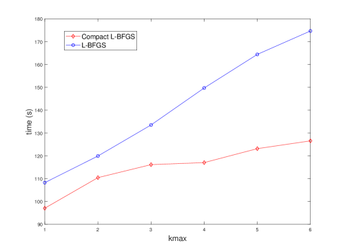
Fig. 1: Bratu problem $n=747003$, $nnz=3\,731023$. Compact vs standard L-BFGS formulas. Initial preconditioner IC(0.01)

Figure 1 shows a comparison between the standard and compact L-BFGS formulas for one of the different discretizations of the Bratu problem tested. It shows clearly that the compact implementation can achieve better computational performance for increasing values of $k_{\max}$, the size of the update window. In our experiments, as it could be expected, it was observed that the difference in performance increases when a large number of linear iterations must be performed, situation that is likely to happen when the nonlinear iteration method is approaching the solution (since in these model problems the ill-conditioning of the jacobians increases toward the end of the Newton process), or when a poor initial preconditioner is used. Similar results where encountered for the other problems tested, also for the L-SR1 formulas. In this case, the gain using the compact formulas is less evident since the number of vectors used to update of the preconditioners is half the number of vectors used with L-BFGS.

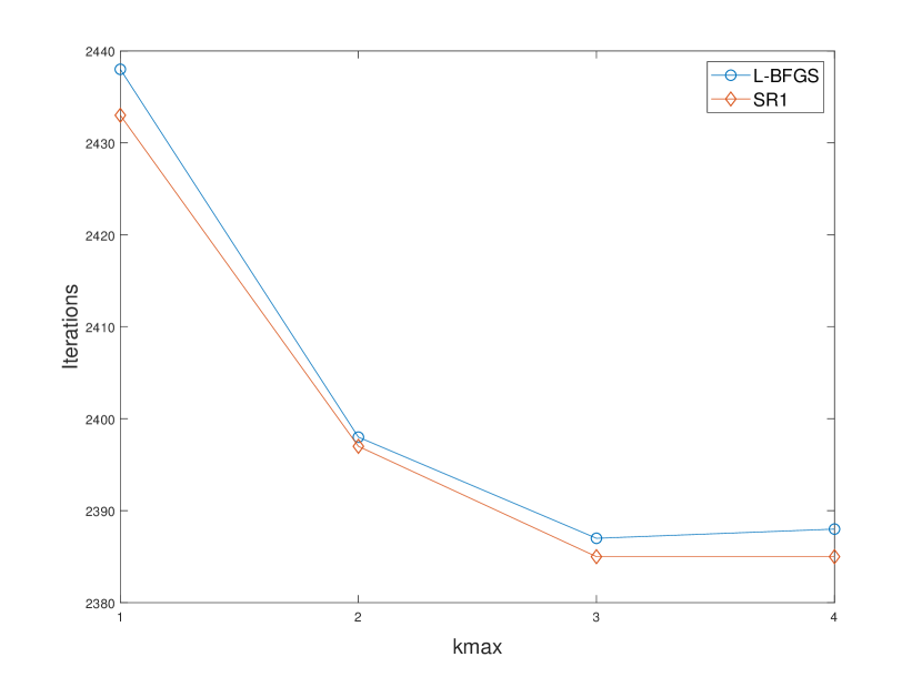
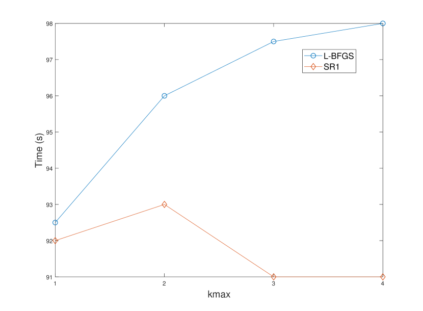
Fig. 2: Compact L-BFGS vs L-SR1. Phi-2 problem $n=747003$, $nnz=3\,731023$. Initial preconditioner IC(0.01)

Figure 2 shows a comparison between the L-BFGS and L-SR1 formulas in their compact version. It is worth to note that the number of iterations spent by the L-SR1 method is similar, or even smaller in many occasions, than the one required by the L-BFGS. This nice behavior gives experimental evidence of the theoretical findings for the SR1 update presented in Section 3. As a consequence, the total computational CPU time spent by the Newton method with the L-SR1 was smaller in all our experiments compared to the L-BFGS formula.

4.2 3d FEM problem

The third problem considered was a modification of the Bratu problem, where the linear term corresponding to the matrix $A$ arises from a 3D Finite Element discretization of Darcy’s law in porous media with heterogeneous hydraulic conductivity coefficient. The size of the problem is $n=268,515$ with a number of nonzero elements $nnz=3\,881337$. For this problem, together IC preconditioning, Jacobi diagonal preconditioning was used to show the effect of starting with a poor preconditioner.

Table 1: Results for 3d FEM problem. Number of nonlinear iterations ${\rm nlit}=15$. Initial preconditioner IC(0.1) – left, Jacobi – right.

preconditioner	$k_{max}$	totlin	CPU
No-update	0	$4\,248$	$66.6$
L-BFGS	1	$3\,703$	$63.5$
	2	$3\,583$	$67.7$
	3	$3\,519$	$69.2$
	4	$3\,513$	$71.1$
L-SR1	1	$3\,673$	$63.7$
	2	$3\,518$	$60.9$
	3	$3\,501$	$62.3$
	4	$3\,493$	$63.2$

preconditioner	$k_{max}$	totlin	CPU
No-update	0	$9\,124$	$133.2$
L-BFGS	1	$7\,779$	$123.9$
	2	$7\,501$	$136.7$
	3	$7\,362$	$138.8$
	4	$7\,339$	$139.4$
L-SR1	1	$7\,781$	$123.6$
	2	$7\,357$	$119.6$
	3	$7\,192$	$119.1$
	4	$7\,197$	$119.2$

Table 1 compares the L-BFGS and L-SR1 methods with initial IC and Jacobi preconditioners and also the no-update case. It can be observed, analogously to the previous problems, that updating by means of the L-SR1 formula yields to the best performance with respect to both total number of linear iterations and CPU time. The time spent to update the preconditioner was negligible compared with the total amount, so it is not indicated. It is worth noting that for these experiments the best results were obtained with $k_{max}=2,3$ when using L-SR1. We finally highlight that in all previous experiments, the SR1 update was always well defined, with the denominator in (11) positive, and the test (28) always satisfied, in all Newton iterations.

4.3 Application to eigenvalue computation

Given an SPD matrix $A$, to compute its leftmost eigenpair, the Newton method in the unit sphere [22] or Newton-Grassmann method, constructs a sequence of vectors $\{\mbox{\boldmath$u$}_{k}\}$ by solving the linear systems

$$J_{k}\mbox{\boldmath$s$}=-\mbox{\boldmath$r$}_{k},\qquad\text{where}\quad J_{k}=(I-\mbox{\boldmath$u$}_{k}\mbox{\boldmath$u$}_{k}^{T})(A-\theta_{k}I)(I-\mbox{\boldmath$u$}_{k}\mbox{\boldmath$u$}_{k}^{T}),$$

$$\mbox{\boldmath$r$}_{k}=-(A\mbox{\boldmath$u$}_{k}-\theta_{k}\mbox{\boldmath$u$}_{k}),\qquad\text{and}\quad\theta_{k}=\dfrac{\mbox{\boldmath$u$}_{k}^{T}A\mbox{\boldmath$u$}_{k}}{\mbox{\boldmath$u$}_{k}^{T}\mbox{\boldmath$u$}_{k}}$$

on a subspace orthogonal to $\mbox{\boldmath$u$}_{k}$. Then the next approximation is set as $\mbox{\boldmath$u$}_{k+1}=\mbox{\boldmath$t$}\|\mbox{\boldmath$t$}\|^{-1}$ where $\mbox{\boldmath$t$}=\mbox{\boldmath$u$}_{k}+\mbox{\boldmath$s$}$. Linear system (4.3) is shown to be better conditioned than the one with $A-\theta_{k}I$. The same linear system represents the correction equation in the well-known Jacobi-Davidson method [23], which in its turn can be viewed as an accelerated Inexact Newton method [24]. When $A$ is SPD and the leftmost eigenpairs are being sought, it has been proved in [21] that the Preconditioned Conjugate Gradient (PCG) method can be employed in the solution of the correction equation. In this work we follow the PCG implementation of [21, Algorithm 5.1].

We tried our updated preconditioners for the PCG solver within the Newton-Grassmann method to compute the leftmost eigenpair of two large and sparse SPD matrices whose characteristics are reported in Table 2. Note that the solution to (4.3) is not needed to be very accurate. We then set as the maximum number of inner CG iterations to 50. The outer Newton process is stopped instead when the following test is satisfied

$$\|A\mbox{\boldmath$u$}_{k}-\theta_{k}\mbox{\boldmath$u$}_{k}\|=\|\mbox{\boldmath$r$}_{k}\|<\theta_{k}10^{-8}.$$

The initial Newton vector has been computed satisfying $\|\mbox{\boldmath$r$}_{k}\|<\theta_{k}10^{-2}$. In both cases the preconditioner is computed once and for all at the beginning of the Newton iteration as an incomplete Cholesky factorization with fill-in of matrix $A$.

Table 2: Main characteristics of the matrices used in the tests.

Matrix	where it comes from	$n$	$nz$	drop tolerance
monte-carlo	2D-MFE stochastic PDE	77120	384320	$10^{-3}$
emilia-923	3D-FE elasticity problem	923136	41 005206	$10^{-5}$

Matrix monte-carlo

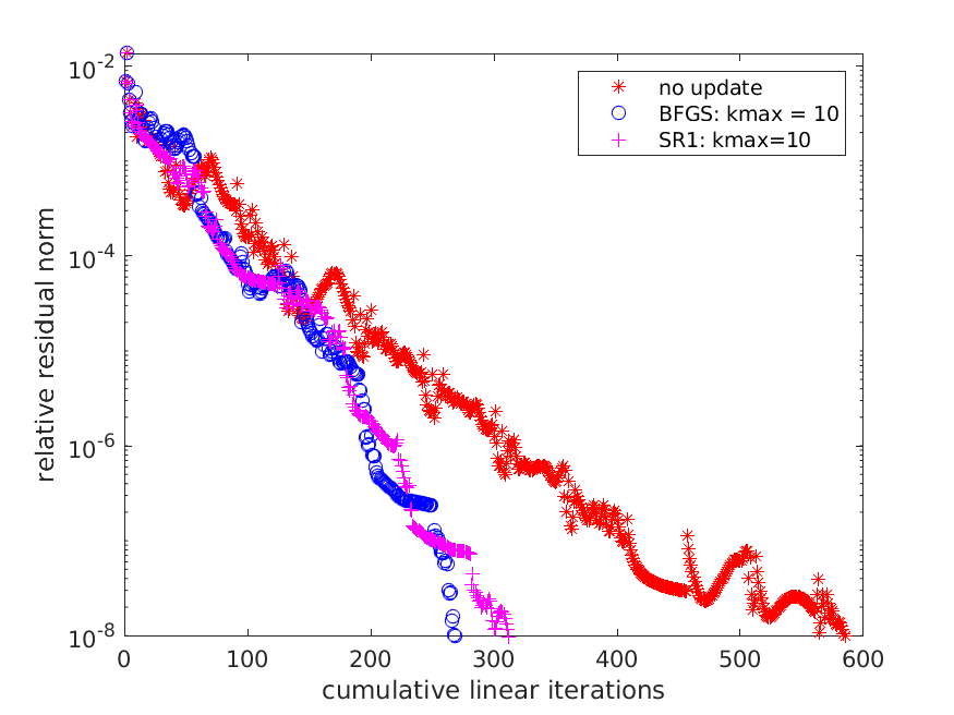
In Table 3 we report the number of outer iterations (nlit) the overall number of the linear iterations (totlin) and the CPU time. We compared the no-update case and the L-BFGS and L-SR1 updates, both with $k_{\max}=\{5,10\}$. Moreover we plot, in Figure 3 the nonlinear relative residual $\|\mbox{\boldmath$r$}_{k}\|\theta_{k}^{-1}$ vs the number of cumulative linear iterations across all the outer Newton iterations.

Table 3: Outer/inner iterations an CPU time to evaluate the leftmost eigenpair of matrix monte-carlo.

	$k_{\max}=10$			$k_{\max}=5$
	nlit	totlin	CPU	nlit	totlin	CPU
L-BFGS	14	269	4.83	15	329	5.66
L-SR1	13	312	4.72	14	340	5.07
No Update	21	585	7.50

Fig. 3: Nonlinear converge profile vs cumulative linear iteration number with different preconditioning strategies. Matrix monte-carlo.

From Table 3 and Figure 3 we can appreciate the remarkable improvement provided by the compact low-rank updates in terms of inner/outer iterations and CPU time. Moreover, once again, the L-SR1 update provides comparable results as the L-BFGS correction being (slightly) the most convenient option in terms of CPU time.

Matrix emilia-923

We report in Table 4 the results for the larger matrix emilia-923 where the L-BFGS acceleration is shown to provide outstanding improvement in both inner/outer iteration number and CPU time, which is also accounted for by Figure 4. The L-SR1 update did not lead to convergence (in fact at nonlinear iteration # 28 the PCG method stopped due to a breakdown).

Table 4: Outer/inner iterations an CPU time to evaluate the leftmost eigenpair of matrix emilia-923. For all the update formulas $k_{\max}=10$ has been set.

	nlit	totlin	CPU
L-BFGS	15	224	183.22
L-SR1 (no scaling)	†	†	†
L-SR1 (with scaling)	16	286	194.82
No Update	21	647	371.20
†: PCG breakdown found at outer iteration # 28.

In the light of Remark 1, to ensure the positive definiteness of the L-SR1 update, we scaled in this case the Cholesky triangular matrix by a factor 1.4, after roughly estimating the largest eigenvalue of $(LL^{T})^{-1}J_{0}$. With this simple modification, the L-SR1 update provides a similar performance as that of the L-BFGS update.

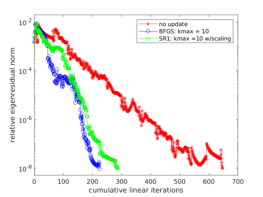
Fig. 4: Nonlinear converge profile vs cumulative linear iteration number with different preconditioning strategies. Matrix emilia-923.

As a general comment, regarding Newton method in eigenvalue computation, the effects of the low-rank updates are much more pronounced as compared to the previous nonlinear problems. Moreover, the relatively high number of nonlinear iterations and the close to indefinite linear systems to be solved at each Newton step suggest the use of higher values of the $k_{\max}$ parameter to improve the properties of the low-rank updates.

5 Conclusions

In this paper a compact version of the rank-two L-BFGS and the rank-one SR1 formulas has been used to update an initial preconditioner for the solution of nonlinear systems within the Inexact Newton methods. One purpose of this study was to show that the compact formulation, which allows application of the preconditioner in matrix form, can improve the performance obtained in the PCG iteration. The other objective of the paper was to show that the rank-one update SR1, despite not being guaranteed to provide SPD preconditioners in all cases, can yet provide SPD sequences by simply scaling the initial (Cholesky) preconditioner. Moreover, it has been shown that the SR1-updated preconditioner is able to shift some eigenvalues towards one, and a bounded deterioration property regarding the condition number of the preconditioned jacobians has been stated.

In practice, the construction of the sequence of preconditioners is based on well known limited memory techniques in order to keep under control the amount of memory, and also the computational time needed to compute and apply the update. From the numerical experiments we can conclude that both the L-BFGS and L-SR1 formulas benefit from the use of compact (block) forms. More interestingly, the experiments have shown that the L-SR1 may be a good alternative to the L-BFGS formula for nonlinear problems with SPD Jacobian. Work is undergoing to provide a parallel implementation of the compact limited memory Quasi-Newton preconditioners to improve a given sparse approximate inverse initial preconditioner in the framework e.g. of sequences of linear systems arising in the eigensolution of very large and sparse matrices in the lines of e.g. [3, 5].

References

• [1] L. Bergamaschi, R. Bru, and A. Martínez, Low-rank update of preconditioners for the inexact Newton method with SPD jacobian, Mathematical and Computer Modelling, 54 (2011), pp. 1863–1873.
• [2] L. Bergamaschi, R. Bru, A. Martínez, and M. Putti, Quasi-Newton preconditioners for the inexact Newton method, Electron. Trans. Numer. Anal., 23 (2006), pp. 76–87.
• [3] L. Bergamaschi and A. Martínez, Parallel RFSAI-BFGS preconditioners for large symmetric eigenproblems, J. Applied Mathematics, 2013, Article ID 767042, 10 pages (2013).
• [4]  , Efficiently preconditioned inexact Newton methods for large symmetric eigenvalue problems, Optimization Methods & Software, 30 (2015), pp. 301–322.
• [5]  , Spectral acceleration of parallel iterative eigensolvers for large scale scientific computing, Advances in Parallel Computing, 32 (2018), pp. 107–116.
• [6] L. Bergamaschi and M. Putti, Mixed finite elements and Newton-type linearization for the solution of Richards equation, Int. J. Numer. Methods Engrg., 45 (1999), pp. 1025–1046.
• [7] R. H. Byrd, J. Nocedal, and R. B. Schnabel, Representations of quasi-Newton matrices and their use in limited memory methods, Mathematical Programming, 63 (1994), pp. 129–156.
• [8] O. DeGuchy, J. B. Erway, and R. F. Marcia, Compact representation of the full Broyden class of quasi-Newton updates, Numerical Linear Algebra with Applications, 25 (2018). e2186.
• [9] R. S. Dembo, S. C. Eisenstat, and T. Steihaug, Inexact Newton methods, SIAM J. Num. Anal., 19 (1982), pp. 400–408.
• [10] M. A. Freitag and A. Spence, A tuned preconditioner for inexact inverse iteration applied to Hermitian eigenvalue problems, IMA J. Numer. Anal., 28 (2008), pp. 522–551.
• [11] G. H. Golub and C. F. van Loan, Matrix Computation, Johns Hopkins University Press, Baltimore, 1991.
• [12] P. Graves-Morris, Personal communication, (2010).
• [13] I. Ipsen and B. Nadler, Refined perturbation bounds for eigenvalues of Hermitian and non-Hermitian matrices, SIAM Journal on Matrix Analysis and Applications, 31 (2009), pp. 40–53.
• [14] C. T. Kelley, Iterative Methods for Linear and Nonlinear Equations, SIAM, Philadelphia, 1995.
• [15] C. T. Kelley, Iterative Methods for Optimization, vol. 18 of Frontiers in Applied Mathematics, SIAM, Philadelphia, PA, 1999.
• [16] A. Martínez, Tuned preconditioners for the eigensolution of large SPD matrices arising in engineering problems, Numer. Lin. Alg. Appl., 23 (2016), pp. 427–443.
• [17] J. M. Martínez, A theory of secant preconditioners, Math. Comp., 60 (1993), pp. 681–698.
• [18] J. L. Morales and J. Nocedal, Automatic preconditioning by limited memory quasi-Newton updating, SIAM J. Optim., 10 (2000), pp. 1079–1096.
• [19] R. Nabben and C. Vuik, A comparison of deflation and the balancing preconditioner, SIAM J. Sci. Comput., 27 (2006), pp. 1742–1759.
• [20] J. Nocedal and S. J. Wright, Numerical optimization, Springer Series in Operations Research, Springer-Verlag, New York, 1999.
• [21] Y. Notay, Combination of Jacobi-Davidson and conjugate gradients for the partial symmetric eigenproblem, Numer. Linear Algebra Appl., 9 (2002), pp. 21–44.
• [22] V. Simoncini and L. Eldén, Inexact Rayleigh quotient-type methods for eigenvalue computations, BIT, 42 (2002), pp. 159–182.
• [23] G. L. G. Sleijpen and H. A. van der Vorst, A Jacobi-Davidson method for linear eigenvalue problems, SIAM J. Matrix Anal. Appl., 17 (1996), pp. 401–425.
• [24] R. A. Tapia, J. E. Dennis, and J. P. Schäfermeyer, Inverse, shifted inverse, and Rayleigh quotient iteration as Newton’s method, SIAM Review, 60 (2018), pp. 3–55.