Double-End Queues with Non-Poisson Inputs and Their Effective Algorithms

Abstract

It is interesting and challenging to study double-ended queues with First-Come-First-Match discipline under customers’ impatient behavior and non-Poisson inputs. The system stability can be guaranteed by the customers’ impatient behavior, while the existence of impatient customers makes analysis of such double-ended queues more difficult or even impossible to find an explicitly analytic solution, thus it becomes more and more important to develop effective numerical methods in a variety of practical matching problems. This paper studies a block-structured double-ended queue, whose block structure comes from two independent Markovian arrival processes (MAPs), which are non-Poisson inputs. We show that such a queue can be expressed as a new bilateral quasi birth-and-death (QBD) process which has its own interest. Based on this, we provide a detailed analysis for both the bilateral QBD process and the double-ended queue, including the system stability, the queue size distributions, the average stationary queue lengths, and the sojourn time of any arriving customers. Furthermore, we develop three effective algorithms for computing the performance measures (i.e., the probabilities of stationary queue lengths, the average stationary queue lengths, and the average sojourn times) of the double-ended queue with non-Poisson inputs. Finally, we use some numerical examples in tabular and graphical to illustrate how the performance measures are influenced by some key system parameters. We believe that the methodology and results described in this paper can be applicable to deal with more general double-ended queues in practice, and develop some effective algorithms for the purpose of many actual uses.

Keywords: Double-ended queue; First-Come-First-Match; impatient customer; Markovian arrival process (MAP); QBD process; RG-factorization.

1 Introduction

In recent years, we are facing more and more matching problems in practice, for example, sharing economy, platform service, multilateral market, organ transplantation, communication network, intelligent manufacturing, transportation networks, and so on. Based on this, it is interesting but difficult and challenging to study double-ended queues with First-Come-First-Match discipline (also known as matched queues) under customers’ impatient behavior and non-Poisson inputs. Note that the stability of this system is guaranteed by customers’ impatient behavior, while the existence of impatient customers always makes analysis of such double-ended queues more difficult or even impossible to find an explicitly analytic solution, thus it becomes more and more important to develop effective numerical methods in a variety of practical matching problems. This motivates us in this paper to develop effective algorithms in a more general double-ended queue with non-Poisson inputs. Therefore, this paper studies a block-structured double-ended queue, whose block structure comes from two independent Markovian arrival processes (MAPs). We show that such a queue can be expressed as a new bilateral QBD process, and provide a detailed analysis for the bilateral QBD process, including the system stability, the queue size distributions, the average stationary queue lengths, and the sojourn time of any arriving customers. Furthermore, we develop three effective algorithms for computing the performance measures (i.e., the probabilities of stationary queue lengths, the average stationary queue lengths, and the average sojourn times) of the double-ended queue with non-Poisson inputs. Finally, numerical examples are employed to illustrate how the performance measures are influenced by key system parameters. We believe that the methodology and results described in this paper can be applicable to deal with more general double-ended queues. Also, this can lead to some new theory of bilateral block-structured Markov processes (e.g., bilateral Markov processes of GI/M/1 type and of M/G/1 type).

Since the double-ended (or matched) queue was first proposed by Kendall (1951), it has received high attention from many practical applications. Important examples include organ transplantation by Zenios (1999), Boxma et al. (2011), Stanford et al. (2014) and Elalouf et al. (2018); taxi issues by Giveen (1961, 1963), Kashyap (1965, 1966, 1967), Bhat (1970), Shi and Lian (2016) and Zhang et al. (2019); sharing economy by Cheng (2016), Sutherland and Jarrahi (2018), Benjaafar and Hu (2019) and Liu et al. (2021); transportation by Browne et al. (1970) and Baik et al. (2002); assembly systems by Hopp and Simon (1989), Som et al. (1994) and Ramachandran and Delen (2005); inventory management by Sasieni (1961), Porteus (1990), and Axsäer (2015); health care by Pandey and Gangeshwer (2018); multimedia synchronization by Steinmetz (1990) and Parthasarathy et al. (1999), and so on.

Recently, an emerging hot research topic focuses on ridesharing platform, which is used to match customers with servers in a bilateral market, for example, transportation, housing, eating, dressing, and so forth. Plenty of research has been conducted in this area, including Azevedo and Weyl (2016), Duenyas et al. (1997), Hu and Zhou (2015), Banerjee and Johari (2019), Braverman et al. (2019), Liu et al. (2021) and so forth. Meanwhile, many ridesharing companies in these areas spring up as a result of rapid development of mobile networks, smart phones and location technologies, such as Uber in transportation, Airbnb in housing, Eatwith in eating, and Rent the Runway in dressing. Observing the ridesharing platform reveals that the match process works as follows: If a customer is in demand of service and makes a request by using his/her smart phone, then the ridesharing platform will try to match the customer with a server. Once such a match is successful, the functioning of the ridesharing platform for this customer is finished immediately. Therefore, the double-ended queue is an effective mathematical method for studying ridesharing platforms, as it is a bilateral matching system or market. Normally, the matching process follows the First-Come–First-Match principle.

Although the double-ended queue seems simple as it contains only a few random factors, its analysis is actually very difficult and challenging due to the fact that the Markov process corresponding to the double-ended queue has a bidirectional state space $\left\{\ldots,-2,-1,0,1,2,\ldots\right\}$. Therefore, up until now, there is still lack of effective methods for conducting performance analysis of double-ended queues. In the early study of double-ended queues, by applying the Markov processes, Sasieni (1961), Giveen (1961) and Dobbie (1961) established the Chapman-Kolmogorov forward differential-difference equations with the bidirectional state space. Also, they introduced customers’ impatient behavior to guarantee system stability. It is well-known that the customers’ impatient behavior further makes analysis of the double-ended queues more difficult and challenging in performance evaluation of the systems due to the level-dependent structure of the corresponding Markov processes, which was discussed in Artalejo and Gómez-Corral (2008) and Li (2010).

When the two waiting rooms of the double-ended queue are both finite, Jain (1962) and Kashyap (1965, 1966, 1967) applied the supplementary variable method to deal with the double-ended queue with a Poisson arrival process and a renewal arrival process. Takahashi et al. (2000), and Takahashi and Takahashi (2000) considered a double-ended queue with a Poisson arrival process and a PH-renewal arrival process. Sharma and Nair (1991) used the matrix theory to analyze the transient behavior of a double-ended Markovian queue.

When the two waiting rooms are both infinite, Latouche (1981) applied the matrix-geometric solution to analyze several different bilateral matching queues with paired input. Conolly et al. (2002) applied the Laplace transform to discuss the time-dependent performance measures of the double-ended queue with state-dependent impatience. Di Crescenzo et al. (2012, 2018) discussed the transient and stationary probability laws of a time-nonhomogeneous double-ended queue with catastrophes and repairs. Diamant and Baron (2019) analyzed a double-ended queue with priority and impatient customers, and derived exact formulae for the stationary queue length distribution and several useful performance measures. Following the matrix-analytic method based on the RG-factorizations, Liu et al. (2020) discussed a double-ended queue with matching batch pair $(m,n)$, which includes two useful examples: Many-to-one and one-to-many matching requests.

When one waiting room is finite while the other one is infinite, Xu et al. (1990) discussed a double-ended queue with two Poisson inputs, a PH service time distribution and a matching proportion $1:r$. They applied the matrix-geometric solution (see Neuts (1981)) to obtain the stable condition of the system, and to analyze the stationary queue lengths of both classes of customers. Further research includes Xu et al. (1993) and Xu and He (1993, 1994). Yuan (1992) applied Markov chains of M/G/1 type (see Neuts (1989)) to consider a double-ended queue with two Poisson inputs, a general service time distribution and a matching proportion $1:r$. Li and Cao (1996) further applied Markov chains of M/G/1 type to deal with a double-ended queue with two batch Markovian arrival processes (BMAPs), a general service time distribution and a matching proportion $1:r$. Wu and He (2020) applied the theory of multi-layer Markov modulated fluid flow (MMFF) processes to analyze a double-sided queueing model with marked Markovian arrival processes and finite discrete abandonment times.

In a double-ended queue, if the two classes of customer arrivals are both general renewal processes, then the ordinary Markov methods (for example, continuous-time Markov chains, the supplementary variable method, the matrix-analytic method and so on) will not work well any more. In this case, the fluid and diffusion approximations become an effective (but approximative) mathematical method to deal with the more general double-ended queues. Jain (2000) applied diffusion approximation to discuss the G${}^{\text{X}}$/G${}^{\text{Y}}$/1 double-ended queue. Di Crescenzo et al. (2012, 2018) discussed a double-ended queue by means of a jump-diffusion approximation. Liu et al. (2014) discussed diffusion models for the double-ended queues with two renewal arrival processes. Büke and Chen (2017) applied fluid and diffusion approximations to study the probabilistic matching systems. Liu (2019) analyzed diffusion approximations for the double-ended queues with reneging in heavy traffic.

Kim et al. (2010) provided a simulation model for a more general double-ended queue. Jain (1995) proposed a sample path analysis for the double-ended queue with time-dependent rates. Afèche et al. (2014) applied the level-crossing method to analyze the double-ended batch queue with abandonment.

Hlynka and Sheahan (1987) analyzed the control rates in a double-ended queue with two Poisson inputs. Gurvich and Ward (2014) discussed dynamic control of the double-ended queues. Büke and Chen (2015) analyzed stabilizing admission control policies for the probabilistic matching systems. Lee et al. (2019) discussed optimal control of a time-varying double-ended production queueing model.

The MAP (Markov arrival process) is a useful mathematical tool, for example, for describing bursty traffic and dependent arrivals in many practical systems, such as computer and communication networks, manufacturing systems, transportation networks and so on. Also, the MAP contains the Poisson process, the PH-renewal process, and the Markovian Modulated Poisson Process as its special cases, e.g., see Section 1.5 of Li (2010). Readers may refer to recent publications for details, among which are Neuts (1979), Chapter 5 in Neuts (1989), Lucantoni (1991), Narayana and Neuts (1992), Chakravarthy (2001), Chapter 1 in Li (2010), Cordeiro and Kharoufeh (2010) and references therein. In the current matching problems (e.g., online bilateral markets, and ride sharing platform), the arrival data flow is always bursty traffic and dependent arrivals. Note that the MAP may be a non-renewal process, and it can express many key features of a practical data flow by means of the statistical adjustment of multiple parameters. Therefore, it is necessary and useful to use the MAP inputs to study the double-ended queues.

To be able to deal with level-dependent (or general) Markov processes, the RG-factorizations were systematically developed in Li (2010). Readers may also refer to, such as, Li and Cao (2004), Li and Liu (2004) and Li and Zhao (2004) for early research. Note that the RG-factorizations were successfully applied to analysis of retrial queues, processor-sharing queues, queues with negative customers, and queues with impatient customers due to their level-dependent Markov processes, thus the RG-factorizations play a key role in the study of double-ended queues whose impatient customers of guaranteeing system stability directly lead to the level-dependent Markov processes. By using the RG-factorizations, this paper finds a feasible solution of the double-ended queue with two MAP inputs and impatient customers, which is more general than those works in the existing literature. Also, we develop some effective RG-factorization algorithms which are able to numerically analyze performance measures of the block-structured double-ended queue.

We summarize the main contributions of this paper as follows:

• We consider a more general block-structured double-ended queue with non-Poisson (MAP) inputs and impatient customers, and show that such a queue can be expressed as a new bilateral QBD process which has its own interest. By using the bilateral QBD process, we can analyze the system stability, the stationary queue lengths and the sojourn times of this double-ended queue. Therefore, we develop a new effective RG-factorization method in the study of double-ended queues, which is different from those in the literature.

• We provide three effective algorithms for computing performance measures of the block-structured matched queue, in which the bilateral level-dependent QBD process is decomposed into two unilateral level-dependent QBD processes that are specifically linked in Level $0$. From the two unilateral level-dependent QBD processes, we can effectively compute the $R$-, $U$- and $G$-measures by means of the those approximate algorithms given in Bright and Taylor (1995, 1997). Based on this, we can numerically compute the stationary queue lengths. Also, we provide an effective method to discuss the sojourn times of the block-structured double-ended queue by using the technique of the first passage times and the PH distributions.

• We use some numerical examples to indicate how the performance measures of the double-ended queue are influenced by key system parameters. In addition, the numerical results are also given a simple and interesting discussion by means of the coupling method of Markov processes.

The structure of this paper is organized as follows. Section 2 describes a double-ended queue with two MAP inputs and customers’ impatient behavior. Section 3 shows that the double-ended queue can be expressed as a new bilateral QBD process. By using the bilateral QBD process, we obtain some stable conditions for the double-ended queues. Section 4 studies the stationary probability vector of the bilateral QBD process, and compute the probabilities of stationary queue lengths and the average stationary queue lengths. Section 5 provides an effective method to discuss the sojourn time of any arriving customer and to compute the average sojourn time by using the technique of the first passage times and the PH distributions. Section 6 uses some numerical examples to indicate how the performance measures of the double-ended queue are influenced by key system parameters, where three effective algorithms are developed. Finally, Section 7 gives some concluding remarks.

2 Model Description

In this section, we describe a more general block-structured double-ended queue with two MAP inputs and customers’ impatient behavior, and also introduce operational mechanism, system parameters and basic notation

In the proposed queue, there are two types of customers, called A-customers and B-customers. Once an A-customer and a B-customer enter their corresponding buffers, they match each other to constitute a pair and leave the queueing system immediately, that is, their matching time is zero. Figure 1 provides a physical illustration for such a double-ended queue.

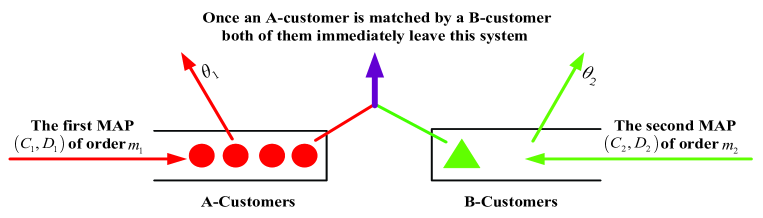
Figure 1: A physical illustration of the double-ended queue

Now, we provide a more detailed description for the double-ended queue as follows:

• The A-customers arrive at the queueing system according to a MAP with irreducible matrix representation $\left(C_{1},D_{1}\right)$ of order $m_{1}$, where $D_{1}\gvertneqq 0$, each diagonal element of $C_{1}$ is negative while its nondiagonal elements are nonnegative, $C_{1}\mathbf{e}\lneqq 0$, $\left(C_{1}+D_{1}\right)\mathbf{e}=0$, and $\mathbf{e}$ is a column vector of ones with a suitable size. We assume that the Markov process $C_{1}+D_{1}$ is irreducible and positive recurrent. Let $\alpha_{1}$ be the stationary probability vector of the Markov process $C_{1}+D_{1}$. Then $\lambda_{1}=\alpha_{1}D_{1}\mathbf{e}$ is the stationary arrival rate of the MAP with irreducible matrix representation $\left(C_{1},D_{1}\right)$.

  Similarly, the B-customers arrive at the queueing system according to a MAP with irreducible matrix representation $\left(C_{2},D_{2}\right)$ of order $m_{2}$, where $D_{2}\gvertneqq 0$, each diagonal element of $C_{2}$ is negative while its nondiagonal elements are nonnegative, $C_{2}\mathbf{e}\lneqq 0$, and $\left(C_{2}+D_{2}\right)\mathbf{e}=0$. We assume that the Markov process $C_{2}+D_{2}$ is irreducible and positive recurrent. Let $\alpha_{2}$ be the stationary probability vector of the Markov process $C_{2}+D_{2}$. Then $\lambda_{2}=\alpha_{2}D_{2}\mathbf{e}$ is the stationary arrival rate of the MAP with irreducible matrix representation $\left(C_{2},D_{2}\right)$.

For the MAPs, readers may refer to Section 1.5 in Chapter 1 of Li [42] for a more detailed introduction.

• If an A-customer (resp. a B-customer) stays in the queueing system for a long time, then she will show some impatience. To capture this phenomenon, we assume that the impatient time, which is defined as the longest time that a customer stays in the buffer before leaving, of an A-customer (resp. a B-customer) is exponentially distributed with impatient rate $\theta_{1}$ (resp. $\theta_{2}$) for $\theta_{1},\theta_{2}>0$.

• Once an A-customer and a B-customer match as a pair, both of them immediately leave the queueing system. The matching process follows a First-Come-First-Match discipline and has the zero matching time. We assume the waiting spaces of A- and B-customers are all infinite.

• We assume that all the random variables defined above are independent of each other.

Finally, we provide some necessary interpretation for some practical factors in the double-ended queue as follows:

(a) The matching times between the A- and B-customers are very short under the current network environment of data exchange and transmission. Thus the matching times are regarded as zero so that the matching of A- and B-customers is complete instantly (or immediately).

(b) The impatient behavior given in Assumption (2) is used to ensure the stability of the double-ended queue, which can be widely found in the real-world situations, such as transportation, housing, eating and so forth.

(c) The matching discipline and the zero matching time given in Assumption (3) indicates that the A- and B-customers cannot simultaneously exist in their corresponding waiting spaces, while such a phenomenon can also be widely found in the real-world situations.

3 A Bilateral QBD Process

In this section, we show that the block-structured double-ended queue can be expressed as a new bilateral QBD process with bidirectional infinite sizes. By using the bilateral QBD process, we obtain some stability conditions of the double-ended queue.

We denote by $N_{1}\left(t\right)$ and $N_{2}\left(t\right)$ the numbers of A- and B-customers in the double-ended queue at time $t\geq 0$, respectively. Let $J_{1}\left(t\right)$ and $J_{2}\left(t\right)$ be the phases of two MAPs for the A- and B-customers at time $t$, respectively. Then the double-ended queue can be modeled as a four-dimensional Markov process $\left\{\left(N_{1}\left(t\right),J_{1}\left(t\right);N_{2}\left(t\right),J_{2}\left(t\right)\right),t\geq 0\right\}$.

For $t\geq 0$, we write all the possible values of $\left(N_{1}\left(t\right),N_{2}\left(t\right)\right)$ as

$$\left\{\ldots,\left(0,3\right),\left(0,2\right),\left(0,1\right),\left(0,0\right),\left(1,0\right),\left(2,0\right),\left(3,0\right),\ldots\right\}.$$

Based on the First-Come-First-Match discipline, it is easy to see that at least one of the two numbers $N_{1}\left(t\right)$ and $N_{2}\left(t\right)$ is zero at any time $t\geq 0$. Let $N\left(t\right)=N_{1}\left(t\right)-N_{2}\left(t\right)$. Then all the possible values of $N\left(t\right)$ for $t\geq 0$ are described as

$$\left\{\ldots,-3,-2,-1,0,1,2,3,\ldots\right\}.$$

Thus, the state transition relations of the Markov process $\left\{\left(N\left(t\right),J_{2}\left(t\right),J_{1}\left(t\right)\right),\text{ }t\geq 0\right\}$ is depicted in Figure 2. It is easy to see from Figure 2 that the Markov process $\{(N\left(t\right),J_{2}\left(t\right)$, $J_{1}\left(t\right)),$ $t\geq 0\}$ is a new bilateral QBD process on a state space, given by

$$\Omega =\left\{\left(n,i,j\right):n\in\left\{\ldots,-2,-1,0,1,2,\ldots\right\},\right.$$

$$\left.i\in\left\{1,2,\ldots,m_{2}\right\},j\in\left\{1,2,\ldots,m_{1}\right\}\right\}.$$

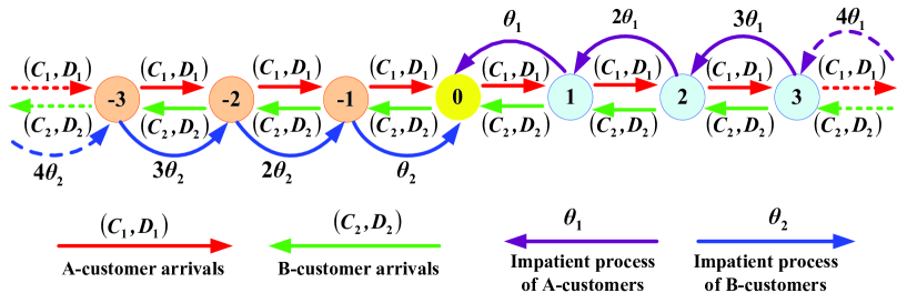
Figure 2: The state transition relations of the bilateral QBD process

Based on Figure 2, the infinitesimal generator of the bilateral QBD process $\{(N\left(t\right),J_{2}\left(t\right)$, $J_{1}\left(t\right)),$ $t\geq 0\}$ is given by

$$Q=\left(\begin{array}[c]{ccccccccccc}\ddots&\ddots&\ddots&&&&&&&&\\ &B_{0}^{\left(-3\right)}&B_{1}^{\left(-3\right)}&B_{2}^{\left(-3\right)}&&&&&&&\\ &&B_{0}^{\left(-2\right)}&B_{1}^{\left(-2\right)}&B_{2}^{\left(-2\right)}&&&&&&\\ &&&B_{0}^{\left(-1\right)}&B_{1}^{\left(-1\right)}&\framebox{$B_{2}^{\left(-1\right)}$}&&&&&\\ &&&&\framebox{$B_{0}^{\left(0\right)}$}&\framebox{$B_{1}^{\left(0\right)}+A_{1}^{\left(0\right)}$}&\framebox{$A_{0}^{\left(0\right)}$}&&&&\\ &&&&&\framebox{$A_{2}^{\left(1\right)}$}&A_{1}^{\left(1\right)}&A_{0}^{\left(1\right)}&&&\\ &&&&&&A_{2}^{\left(2\right)}&A_{1}^{\left(2\right)}&A_{0}^{\left(2\right)}&&\\ &&&&&&&A_{2}^{\left(3\right)}&A_{1}^{\left(3\right)}&A_{0}^{\left(3\right)}&\\ &&&&&&&&\ddots&\ddots&\ddots\end{array}\right)$$ (1)

where

$$A_{1}^{\left(0\right)}=I\otimes C_{1},\text{ \ }B_{1}^{\left(0\right)}=C_{2}\otimes I,$$

$$A_{0}^{\left(k\right)}=I\otimes D_{1},\text{ \ }k\geq 0,$$

$$A_{1}^{\left(k\right)}=C_{2}\oplus C_{1}-k\theta_{1}I,\text{ }A_{2}^{\left(k\right)}=D_{2}\otimes I+k\theta_{1}I,\text{ \ }k\geq 1,$$

$$B_{0}^{\left(k\right)}=D_{2}\otimes I,\text{ \ }k\leq 0,$$

$$B_{1}^{\left(k\right)}=C_{2}\oplus C_{1}+k\theta_{2}I,\text{ }B_{2}^{\left(k\right)}=I\otimes D_{1}-k\theta_{2}I,\text{ \ }k\leq-1.$$

where $\oplus$ and $\otimes$ are the Kronecker sum and the Kronecker product for two matrices, respectively.

Now, the key is how to discuss the new bilateral QBD process $Q$, which is an interesting issue in the study of stochastic models. Note that such a bilateral QBD process was first introduced in Latouche (1981) and further analyzed in Li and Cao (2004).

To analyze the double-ended queue, it is observed that Level $0$, together with the suitable block decomposition $B_{1}^{\left(0\right)}+A_{1}^{\left(0\right)}$, plays a key role, where

$$\text{Level }0= \left\{\left(0,1,1\right),\left(0,1,2\right),\ldots,\left(0,1,m_{1}\right);\left(0,2,1\right),\left(0,2,2\right),\ldots,\left(0,2,m_{1}\right);\right.$$

$$\left.\ldots;\left(0,m_{2},1\right),\left(0,m_{2},2\right),\ldots,\left(0,m_{2},m_{1}\right)\right\}.$$

By using the block decomposition $B_{1}^{\left(0\right)}+A_{1}^{\left(0\right)}$, we divide the bilateral QBD process $Q$ into two unilateral QBD processes: $Q_{A}$ and $Q_{B}$, both of which are interlinked from two different state space directions (upward and downward, respectively) by means of Level $0$ with the blocks $A_{1}^{\left(0\right)}$ and $A_{0}^{\left(0\right)}$, and the blocks $B_{1}^{\left(0\right)}$ and $B_{0}^{\left(0\right)}$, respectively. Thus the infinitesimal generators of the two unilateral QBD processes are respectively given by

$$Q_{A}=\left(\begin{array}[c]{ccccccc}A_{1}^{\left(0\right)}&A_{0}^{\left(0\right)}&&&&&\\ A_{2}^{\left(1\right)}&A_{1}^{\left(1\right)}&A_{0}^{\left(1\right)}&&&&\\ &A_{2}^{\left(2\right)}&A_{1}^{\left(2\right)}&A_{0}^{\left(2\right)}&&&\\ &&A_{2}^{\left(3\right)}&A_{1}^{\left(3\right)}&A_{0}^{\left(3\right)}&&\\ &&&A_{2}^{\left(4\right)}&A_{1}^{\left(4\right)}&A_{0}^{\left(4\right)}&\\ &&&&\ddots&\ddots&\ddots\end{array}\right)$$

and

$$Q_{B}=\left(\begin{array}[c]{ccccccc}B_{1}^{\left(0\right)}&B_{0}^{\left(0\right)}&&&&&\\ B_{2}^{\left(-1\right)}&B_{1}^{\left(-1\right)}&B_{0}^{\left(-1\right)}&&&&\\ &B_{2}^{\left(-2\right)}&B_{1}^{\left(-2\right)}&B_{0}^{\left(-2\right)}&&&\\ &&B_{2}^{\left(-3\right)}&B_{1}^{\left(-3\right)}&B_{0}^{\left(-3\right)}&&\\ &&&B_{2}^{\left(-4\right)}&B_{1}^{\left(-4\right)}&B_{0}^{\left(-4\right)}&\\ &&&&\ddots&\ddots&\ddots\end{array}\right).$$

In the remainder of this section, we analyze the stability of the double-ended queue by means of that of the two unilateral QBD processes $Q_{A}$ and $Q_{B}$, because the bilateral QBD process $Q$ can be divided into the two unilateral QBD processes with $Q_{A}$ and $Q_{B}$.

The following lemma provides useful relations of stability among the bilateral QBD process $Q$ and the two unilateral QBD processes $Q_{A}$ and $Q_{B}$. Its proof is quite straightforward and is omitted here for brevity.

Lemma 1.

To study the stability of the bilateral QBD process $Q$, we have

(a) The bilateral QBD process $Q$ is positive recurrent if the two QBD processes $Q_{A}$ and $Q_{B}$ are both positive recurrent.

(b) The bilateral QBD process $Q$ is null recurrent if the QBD process $Q_{A}$ is recurrent and the QBD process $Q_{B}$ is null recurrent; or the QBD process $Q_{A}$ is null recurrent and the QBD process $Q_{B}$ is recurrent.

(c) The bilateral QBD process $Q$ is transient if at least one of the two QBD processes $Q_{A}$ and $Q_{B}$ is transient.

It is worth noting that the impatience of the two classes of customers plays a key role in guaranteeing the stability of the double-ended queue (or bilateral QBD process), in which we consider three different cases: $\left(\theta_{1},\theta_{2}\right)>0$; $\left(\theta_{1},\theta_{2}\right)=0$; and either $\theta_{1}>0,\theta_{2}=0$ or $\theta_{1}=0,\theta_{2}>0$. From the three cases, we use Lemma 1 to conduct some simple analysis.

The following theorem provides a necessary and sufficient condition for the stability of the block-structured double-ended queue with $\left(\theta_{1},\theta_{2}\right)>0$.

Theorem 1.

If $\left(\theta_{1},\theta_{2}\right)>0$, then the bilateral QBD process $Q$ must be irreducible and positive recurrent. Thus the block-structured double-ended queue is stable.

Proof. Please see (a) Proof of Theorem 1 in the appendix.

Remark 1.

Theorem 1 shows that the stability of the block-structured double-ended queue depends on only the two impatient rates $\theta_{1},\theta_{2}>0$, and has nothing to do with the two MAP inputs. This is true through comparing the rate of the upward shift with the rate of the downward shift from some levels, and further by using the mean drift method for the stability of Markov processes, e.g., see Li [42].

In what follows we consider the influence of the two impatient rates $\theta_{1}$ and $\theta_{2}$ on the stability of the system.

For $\theta_{1}=\theta_{2}=0$, we discuss the stable conditions of the bilateral QBD process related to the double-ended queue.

Corollary 2.

Suppose $\theta_{1}=\theta_{2}=0$.

(1) If $\lambda_{1}\neq\lambda_{2}$, then the bilateral QBD process $Q$ is transient, and the double-ended queue is also transient.

(2) If $\lambda_{1}=\lambda_{2}$, then the bilateral QBD process $Q$ is null recurrent, and the double-ended queue is also null recurrent.

Proof. (1) Since $\lambda_{1}\neq\lambda_{2}$, we shown only the case with $\lambda_{1}>\lambda_{2}$; while the case with $\lambda_{1}<\lambda_{2}$ can be dealt with similarly.

Note that, when $\theta_{1}=\theta_{2}=0$ and $\lambda_{1}>\lambda_{2}$, it is easy to see that the QBD process $Q_{A}$ is transient and the QBD process $Q_{B}$ is positive recurrent. Thus the bilateral QBD process $Q$ is transient, so that the double-ended queue is also transient.

(2) Note that, when $\theta_{1}=\theta_{2}=0$ and $\lambda_{1}=\lambda_{2}$, it is easy to see that the QBD processes $Q_{A}$ and $Q_{B}$ are both null recurrent. Thus the bilateral QBD process $Q$ is null recurrent, so that the double-ended queue is also null recurrent. This completes the proof. $\blacksquare$

Finally, we consider the case with either $\theta_{1}>0$ and $\theta_{2}=0$ or $\theta_{1}=0$ and $\theta_{2}>0$.

The following corollary only considers the case with $\theta_{1}>0$ and $\theta_{2}=0$; while another case with $\theta_{1}=0$ and $\theta_{2}>0$ can be analyzed similarly and is omitted for brevity.

Corollary 3.

Suppose $\theta_{1}>0$ and $\theta_{2}=0$.

(1) If $\lambda_{1}=\lambda_{2}$, then the bilateral QBD process $Q$ is null recurrent, and the double-ended queue is also null recurrent.

(2) If $\lambda_{1}>\lambda_{2}$, then the bilateral QBD process $Q$ is positive recurrent, and the double-ended queue is also positive recurrent.

(3) If $\lambda_{1}<\lambda_{2}$, then the bilateral QBD process $Q$ is transient, and the double-ended queue is also transient.

Proof. (1) If $\lambda_{1}=\lambda_{2}$, $\theta_{1}>0$ and $\theta_{2}=0$, then the QBD process $Q_{A}$ is positive recurrent while the QBD process $Q_{B}$ is null recurrent. Thus, the bilateral QBD process $Q$ is null recurrent, so that the double-ended queue is also null recurrent.

(2) If $\lambda_{1}>\lambda_{2}$, $\theta_{1}>0$ and $\theta_{2}=0$, then the QBD processes $Q_{A}$ and $Q_{B}$ are both positive recurrent. Thus, the bilateral QBD process $Q$ is positive recurrent, so that the double-ended queue is also positive recurrent.

(3) If $\lambda_{1}<\lambda_{2}$, $\theta_{1}>0$ and $\theta_{2}=0$, then the QBD process $Q_{A}$ is positive recurrent while the QBD process $Q_{B}$ is transient. Thus, the bilateral QBD process $Q$ is transient, so that the double-ended queue is also transient. This completes the proof. $\blacksquare$

Remark 2.

From Corollary 2, it is seen that if $\theta_{1}=\theta_{2}=0$, then the double-ended queue can not be positive recurrent. To guarantee the stability of the double-ended queue, we must introduce the impatient customers, i.e., $\theta_{1}>0$ or $\theta_{2}>0$. This is given a detailed analysis in Theorem 1 for $\theta_{1}>0$ and $\theta_{2}>0$; and Corollary 3 for either $\theta_{1}>0$ and $\theta_{2}=0$, or $\theta_{1}=0$ and $\theta_{2}>0$.

4 The Stationary Queue Length

In this section, we first provide a matrix-product expression for the stationary probability vector of the bilateral QBD process by means of the RG-factorizations. Then we provide performance analysis of the block-structured double-ended queue.

We write

$$p_{k;i,j}\left(t\right)=P\left\{N\left(t\right)=k;\text{ \ }J_{2}\left(t\right)=i,J_{1}\left(t\right)=j\right\}.$$

Since the bilateral QBD process is stable, we have

$$\pi_{k;i,j}=\lim_{t\rightarrow+\infty}p_{k;i,j}\left(t\right).$$

For any integer $k=\ldots,-2,-1,0,1,2,\ldots$, we write

$$\pi_{k}=\left(\pi_{k;1,1},\pi_{k;1,2},\ldots,\pi_{k;1,m_{1}};\pi_{k;2,1},\pi_{k;2,2},\ldots,\pi_{k;2,m_{1}};\ldots;\pi_{k;m_{2},1},\pi_{k;m_{2},2},\ldots,\pi_{k;m_{2},m_{1}}\right)$$

and

$$\pi=\left(\ldots,\pi_{-2},\pi_{-1},\pi_{0},\pi_{1},\pi_{2},\ldots\right).$$

To compute the stationary probability vector of the bilateral QBD process $Q$, we first need to compute the stationary probability vectors of the two unilateral QBD processes $Q_{A}$ and $Q_{B}$. Then we use Levels $1$, $0$ and $-1$ to determine the stationary probability vectors on the interaction boundary (i.e., Levels $1$, $0$ and $-1$) of the bilateral QBD process $Q$.

Note that the two unilateral QBD processes $Q_{A}$ and $Q_{B}$ are level-dependent, thus we need to apply the RG-factorizations given in Li (2010) to calculate their stationary probability vectors. To this end, we need to introduce the UL-type $U$-, $R$- and $G$-measures for the two unilateral QBD processes $Q_{A}$ and $Q_{B}$, respectively. In fact, an early analysis for such a level-dependent QBD process was given in Ramaswami and Taylor (1996) and Li and Cao (2004).

For the unilateral QBD process $Q_{A}$, we define the UL-type $U$-, $R$- and $G$-measures as

$$U_{k}=A_{1}^{\left(k\right)}+A_{0}^{\left(k\right)}\left(-U_{k+1}^{-1}\right)A_{2}^{\left(k+1\right)},\text{ \ }k\geq 0,$$ (2)

$$R_{k}=A_{0}^{\left(k\right)}\left(-U_{k+1}^{-1}\right),\text{ \ }k\geq 0,$$

and

$$G_{k}=\left(-U_{k}^{-1}\right)A_{2}^{\left(k\right)},\text{ \ }k\geq 1.$$

On the other hand, it is well-known from Ramaswami and Taylor (1996) that the matrix sequence $\left\{R_{k},k\geq 0\right\}$ is the minimal nonnegative solution to the system of nonlinear matrix equations

$$A_{0}^{\left(k\right)}+R_{k}A_{1}^{\left(k+1\right)}+R_{k}R_{k+1}A_{2}^{\left(k+2\right)}=0,\text{ \ }k\geq 0,$$ (3)

and the matrix sequence $\left\{G_{k},k\geq 1\right\}$ is the minimal nonnegative solution to the system of nonlinear matrix equations

$$A_{0}^{\left(k\right)}G_{k+1}G_{k}+A_{1}^{\left(k\right)}G_{k}+A_{2}^{\left(k\right)}=0,\text{ \ }k\geq 1.$$ (4)

Once the matrix sequence $\left\{R_{k},k\geq 0\right\}$ or $\left\{G_{k},k\geq 1\right\}$ is given, for $k\geq 0$ we have

$$U_{k} =A_{1}^{\left(k\right)}+A_{0}^{\left(k\right)}\left(-U_{k+1}^{-1}\right)A_{2}^{\left(k+1\right)}$$

$$=A_{1}^{\left(k\right)}+R_{k}A_{2}^{\left(k+1\right)}$$

$$=A_{1}^{\left(k\right)}+A_{0}^{\left(k\right)}G_{k+1}.$$

For the unilateral QBD process $Q_{A}$, by following the method described in Chapter 1 of Li (2010) or Li and Cao (2004), the UL-type RG-factorization is given by

$$Q_{A}=\left(I-R_{U}\right)U_{D}\left(I-G_{L}\right),$$ (5)

where

$$U_{D}=\text{diag}\left(U_{0},U_{1},U_{2},U_{3},\ldots\right),$$

$$R_{U}=\left(\begin{array}[c]{ccccc}0&R_{0}&&&\\ &0&R_{1}&&\\ &&0&R_{2}&\\ &&&0&\ddots\\ &&&&\ddots\end{array}\right),\text{ \ \ \ }G_{L}=\left(\begin{array}[c]{ccccc}0&&&&\\ G_{1}&0&&&\\ &G_{2}&0&&\\ &&G_{3}&0&\\ &&&\ddots&\ddots\end{array}\right).$$

Let $\pi_{A}=\left(\pi_{0}^{A},\pi_{1}^{A},\pi_{2}^{A},\ldots\right)$ be the stationary probability vector of the unilateral QBD process $Q_{A}$. Then by applying the UL-type RG-factorization and using the $R$-measure $\left\{R_{k}:k\geq 1\right\}$, we have

$$\pi_{k}^{A}=\pi_{1}^{A}R_{1}R_{2}\cdots R_{k-1},\text{ \ }k\geq 2.$$ (6)

By conducting a similar analysis to that shown above, we can set up the stationary probability vector, $\pi_{B}=\left(\pi_{0}^{B},\pi_{1}^{B},\pi_{2}^{B},\ldots\right)$, of the unilateral QBD process $Q_{B}$. Here, we only provide the $R$-measure $\left\{\mathbb{R}_{k}:k\leq 0\right\}$, while the $U$-measure $\left\{\mathbb{U}_{k}:k\leq 0\right\}$ and $G$-measure $\left\{\mathbb{G}_{k}:k\leq-1\right\}$ can be given easily and is omitted for brevity.

Let the matrix sequence $\left\{\mathbb{R}_{k},k\leq 0\right\}$ be the minimal nonnegative solution to the system of nonlinear matrix equations

$$B_{0}^{\left(k\right)}+\mathbb{R}_{k}B_{1}^{\left(k-1\right)}+\mathbb{R}_{k}\mathbb{R}_{k-1}B_{2}^{\left(k-2\right)}=0,\text{ }k\leq 0,$$ (7)

By using the $R$-measure $\left\{\mathbb{R}_{k}:k\leq-1\right\}$, we obtain

$$\pi_{k}^{B}=\pi_{-1}^{B}\mathbb{R}_{-1}\mathbb{R}_{-2}\cdots\mathbb{R}_{k+1},\text{ \ }k\leq-2.$$ (8)

Remark 3.

In the above analysis, one of the main purposes of applying the UL-type RG-factorization is to show that our computational procedures can be easily extended and generalized to deal with more general bilateral block-structured Markov processes, such as bilateral Markov processes of M/G/1 type, bilateral Markov processes of GI/M/1 type and so on. See Chapter 1 in Li (2010) for more details.

The following theorem expresses the stationary probability vector $\pi=\left(\ldots,\pi_{-2},\pi_{-1},\right.$

$\left.\pi_{0},\pi_{1},\pi_{2},\ldots\right)$ of the bilateral QBD process $Q$ in terms of the stationary probability vectors: $\pi_{A}=\left(\pi_{2}^{A},\pi_{3}^{A},\pi_{4}^{A},\ldots\right)$ given in (6), and $\pi_{B}=\left(\pi_{-2}^{B},\pi_{-3}^{B},\pi_{-4}^{B},\ldots\right)$ given in (8).

Theorem 4.

The stationary probability vector $\pi$ of the bilateral QBD process $Q$ is given by

$$\pi_{k}=c\widetilde{\pi}_{k},$$ (9)

and

$$\widetilde{\pi}_{k}=\left\{\begin{array}[c]{l}\widetilde{\pi}_{-1}\mathbb{R}_{-1}\mathbb{R}_{-2}\cdots\mathbb{R}_{k+1},\text{ }k\leq-2,\\ \widetilde{\pi}_{-1},\\ \widetilde{\pi}_{0},\\ \widetilde{\pi}_{1},\\ \widetilde{\pi}_{1}R_{1}R_{2}\cdots R_{k-1},\text{ \ }k\geq 2,\end{array}\right.$$ (10)

where the three vectors $\widetilde{\pi}_{-1},\widetilde{\pi}_{0},\widetilde{\pi}_{1}$ are uniquely determined by the following system of linear equations

$$\left\{\begin{array}[c]{l}\widetilde{\pi}_{-1}\mathbb{R}_{-1}B_{2}^{\left(-2\right)}+\widetilde{\pi}_{-1}B_{1}^{\left(-1\right)}+\widetilde{\pi}_{0}B_{0}^{\left(0\right)}=0,\\ \widetilde{\pi}_{-1}B_{2}^{\left(-1\right)}+\widetilde{\pi}_{0}\left(B_{1}^{\left(0\right)}+A_{1}^{\left(0\right)}\right)+\widetilde{\pi}_{1}A_{2}^{\left(1\right)}=0,\\ \widetilde{\pi}_{0}A_{0}^{\left(0\right)}+\widetilde{\pi}_{1}A_{1}^{\left(1\right)}+\widetilde{\pi}_{1}R_{1}A_{2}^{\left(2\right)}=0,\end{array}\right.$$ (11)

and the positive constant $c$ is uniquely given by

$$c=\frac{1}{\sum_{k\leq-2}\widetilde{\pi}_{-1}\mathbb{R}_{-1}\mathbb{R}_{-2}\cdots\mathbb{R}_{k+1}\mathbf{e}+\widetilde{\pi}_{-1}\mathbf{e}+\widetilde{\pi}_{0}\mathbf{e}+\widetilde{\pi}_{1}\mathbf{e}+\sum_{k=2}^{\infty}\widetilde{\pi}_{1}R_{1}R_{2}\cdots R_{k-1}\mathbf{e}}.$$ (12)

Proof. Please see (a) Proof of Theorem 4 in the appendix.

Remark 4.

(a) Just like Markovian retrial queues, analysis of queues with impatient customers is in the face of level-dependent Markov processes, hence it is difficult and challenging to have an explicit analytical expression for their stationary probabilities.

(b) The retrial customers change the arrival process to be state-dependent; while the impatient customers make the service process to be state-dependent. Thus both of them lead to the level-dependent Markov processes whose analysis is completed by means of almost the only way: RG-factorizations. See Chapter 2 of Li (2010) and some remarks in Chapter 5 of Artalejo and Gómez-Corral (2008). Also, the stationary probability vector is always expressed as the matrix-product solution.

In the remainder of this section, we provide performance analysis of the block-structured double-ended queue by means of the stationary probability vector of the bilateral QBD process.

Note that the block-structured double-ended queue must be stable for $\left(\theta_{1},\theta_{2}\right)>0$. Thus, we denote by $\mathcal{Q},\mathcal{Q}^{\left(1\right)}$ and $\mathcal{Q}^{\left(2\right)}$ the stationary queue lengths of the double-ended queue, the A- and B-customers, respectively.

By using Theorem 4, we can provide some useful performance measures as follows:

(a) A stationary queue length is zero

The stationary probability that there is no A-customer is given by

$$P\left\{\mathcal{Q}^{\left(1\right)}=0\right\}=\sum_{k\leq 0}\pi_{k}\mathbf{e}.$$

The stationary probability that there is no B-customer is given by

$$P\left\{\mathcal{Q}^{\left(2\right)}=0\right\}=\sum_{k=0}^{\infty}\pi_{k}\mathbf{e}.$$

The stationary probability that there is neither A-customer nor B-customer is given by

$$P\left\{\mathcal{Q}=0\right\}=P\left\{\mathcal{Q}^{\left(1\right)}=0\text{ and }\mathcal{Q}^{\left(2\right)}=0\right\}=\pi_{0}\mathbf{e}.$$

(b) The average stationary queue lengths

$$E\left[\mathcal{Q}\right]= E\left[\mathcal{Q}\text{ }|\text{ }\mathcal{Q}^{\left(1\right)}>0,\mathcal{Q}^{\left(2\right)}=0\right]P\left\{\mathcal{Q}^{\left(1\right)}>0\right\}$$

$$+E\left[\mathcal{Q}\text{ }|\text{ }\mathcal{Q}^{\left(2\right)}>0,\mathcal{Q}^{\left(1\right)}=0\right]P\left\{\mathcal{Q}^{\left(2\right)}>0\right\}$$

$$= E\left[\mathcal{Q}^{\left(1\right)}\right]P\left\{\mathcal{Q}^{\left(1\right)}>0\right\}+E\left[\mathcal{Q}^{\left(2\right)}\right]P\left\{\mathcal{Q}^{\left(2\right)}>0\right\},$$

where

$$E\left[\mathcal{Q}^{\left(1\right)}\right] =\sum_{k=1}^{\infty}k\pi_{k}\mathbf{e}=\sum_{k=1}^{\infty}kc\widetilde{\pi}_{k}\mathbf{e}$$

$$=c\widetilde{\pi}_{1}\mathbf{e+}\sum_{k=2}^{\infty}kc\widetilde{\pi}_{1}R_{1}R_{2}\cdots R_{k-1}\mathbf{e,}$$

$$P\left\{\mathcal{Q}^{\left(1\right)}>0\right\}=\sum_{k=1}^{\infty}\pi_{k}\mathbf{e=}c\widetilde{\pi}_{1}\mathbf{e+}\sum_{k=2}^{\infty}c\widetilde{\pi}_{1}R_{1}R_{2}\cdots R_{k-1}\mathbf{e,}$$

and

$$E\left[\mathcal{Q}^{\left(2\right)}\right] =\sum_{k\leq-1}\left(-k\right)\pi_{k}\mathbf{e}=\sum_{k\leq-1}\left(-k\right)c\widetilde{\pi}_{k}\mathbf{e}$$

$$=c\widetilde{\pi}_{-1}\mathbf{e+}\sum_{k\leq-2}\left(-k\right)c\widetilde{\pi}_{-1}\mathbb{R}_{-1}\mathbb{R}_{-2}\cdots\mathbb{R}_{k+1}\mathbf{e,}$$

$$P\left\{\mathcal{Q}^{\left(2\right)}>0\right\}=\sum_{k\leq-1}\pi_{k}\mathbf{e}=c\widetilde{\pi}_{-1}\mathbf{e+}\sum_{k\leq-2}c\widetilde{\pi}_{-1}\mathbb{R}_{-1}\mathbb{R}_{-2}\cdots\mathbb{R}_{k+1}\mathbf{e.}$$

5 The Sojourn Time

In this section, we provide an effective method for analyzing the sojourn time of any arriving customer, and for computing the average sojourn time.

Note that analysis of the sojourn times is symmetrical and similar in the double-ended queue, thus our discussion mainly focuses on the sojourn time of an arriving A-customer, while that of an arriving B-customer can be dealt with similarly.

In the double-ended queue, the sojourn time is the time interval from the arrival epoch of a customer to its departure time. Let $W_{A}^{\left(k\right)}$ be the sojourn time of an arriving A-customer that there are $k-1$ A-customers in front of her at the moment of her arrival for $k\geq 1$. For convenience of computation, we assume that the arrival moment of this A-customer is time $0$.

If the arriving A-customer finds $k-1$ A-customers in front of her at time $0$ (i.e., the moment of her arrival), then we denote by $N_{1}\left(t\right)$ the number of A-customers in the system at time $t\geq 0$, and by $M\left(t\right)$ the number of A-customers waiting for the matching service in front of the arriving A-customer at time $t$. Let $J_{2}\left(t\right)$ be the phase of the MAP of the B-customers at time $t$.

From the model descriptions, it is easy to see that $\left\{\left(N_{1}\left(t\right),M\left(t\right),J_{2}\left(t\right)\right),t\geq 0\right\}$ is a Markov process with an absorption state $\Delta$, where $\Delta$ denotes such a state that this arriving A-customer leaves the double-ended queue. Thus, the state transition relations of the Markov process are depicted in Figure 3, in which $J_{2}\left(t\right)$ are ignored for the sake of simplicity.

It is obvious that the sojourn time $W_{A}^{\left(k\right)}$ is the first passage time that the Markov process $\left\{\left(N_{1}\left(t\right),M\left(t\right),J_{2}\left(t\right)\right),t\geq 0\right\}$ arrives at the absorption state $\Delta$ for the first time. Note that the Markov process starts at state $\left(k,k-1\right)$ at time $0$.

From Figure 3, the state space of the Markov process with the absorption state $\Delta$ is given by

$$\Xi=\left\{\Delta\right\}\cup\left\{\left(k-i,k-i-1\right):i=0,1,\ldots,k-1\right\}.$$

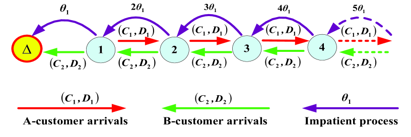
Figure 3: The state transition relations of the Markov process with the absorption state $\Delta$

From Figure 3 and the state space $\Xi$, it is easy to check that the infinitesimal generator of the Markov process with the absorption state $\Delta$ is given by

$$\Theta=\left(\begin{array}[c]{cc}0&\mathbf{0}\\ T^{0}&T\end{array}\right),$$ (13)

where $T\mathbf{e}+T^{0}=0$,

$$T^{0}=\left(\begin{array}[c]{c}T_{k}^{0}\\ T_{k-1}^{0}\\ \vdots\\ T_{3}^{0}\\ T_{2}^{0}\\ T_{1}^{0}\end{array}\right),T=\left(\begin{array}[c]{cccccc}T_{k,k}&T_{k,k-1}&&&&\\ &T_{k-1,k-1}&T_{k-1,k-2}&&&\\ &&\ddots&\ddots&&\\ &&&T_{3,3}&T_{3,2}&\\ &&&&T_{2,2}&T_{2,1}\\ &&&&&T_{1,1}\end{array}\right),$$

$$T_{i}^{0}=\theta_{1}I,i=k,\ldots,2,\text{ \ }T_{1}^{0}=D_{2}+\theta_{1}I,$$

for $j=k,k-1\ldots,2,1,$

$$T_{j,j}=C_{2}-j\theta_{1}I$$

and for $i=k,k-1\ldots,3,2,$

$$T_{i,i-1}=D_{2}+\left(i-1\right)\theta_{1}I\mathbf{.}$$

Let $\left(\alpha_{\Delta},\overrightarrow{\alpha}\right)$ denote the initial probability vector of the Markov process $\Theta$ with the absorption state $\Delta$, $\alpha_{\Delta}=0$, $\overrightarrow{\alpha}=\left(\alpha_{2},\mathbf{0},\ldots,\mathbf{0},\mathbf{0}\right)$, where $\alpha_{2}$ is the stationary probability vector of the Markov process $C_{2}+D_{2}$. Note that the initial probability vector $\left(\alpha_{\Delta},\overrightarrow{\alpha}\right)$ shows that the Markov process $\Theta$ begins at state $\left(k,k-1\right)$ with the phase probability vector $\alpha_{2}$ of the MAP with irreducible matrix representation $\left(C_{2},D_{2}\right)$.

The following theorem uses the phase-type distribution to provide expression for the probability distribution of the sojourn time $W_{A}^{\left(k\right)}$.

Theorem 5.

The probability distribution of the sojourn time $W_{A}^{\left(k\right)}$ is of phase-type with an irreducible representation $\left(\overrightarrow{\alpha},T\right)$ of order $km_{2}$, and

$$F\left(t\right)=P\left\{W_{A}^{\left(k\right)}\leq t\right\}=1-\overrightarrow{\alpha}\exp\left\{Tt\right\}\mathbf{e,}\text{ \ }t\geq 0.$$

Also, the average sojourn time $W_{A}^{\left(k\right)}$ is given by

$$E\left[W_{A}^{\left(k\right)}\right]=-\overrightarrow{\alpha}T^{-1}\mathbf{e}.$$

Proof. For $\left(m,n\right)\in\left\{\left(k-i,k-i-1\right):i=0,1,\ldots,k-1\right\}$ and $j_{2}\in\left\{1,2,\ldots,m_{2}\right\}$, we write

$$q_{m,n;j_{2}}\left(t\right)=P\left\{M\left(t\right)=m,N_{1}\left(t\right)=n;\text{ }J_{2}\left(t\right)=j_{2}\right\},$$

which is the state probability that the Markov process $\Theta$ with the absorbing state $\Delta$ is at state $\left(m,n;j_{2}\right)$ at time $t\geq 0$ before absorbed to state $\Delta$. We write

$$\mathbf{q}_{m,n}\left(t\right)=\left(q_{m,n;1}\left(t\right),q_{m,n;2}\left(t\right),\ldots,q_{m,n;m_{2}}\left(t\right)\right),$$

$$\overrightarrow{\mathbf{q}}\left(t\right)=\left(\mathbf{q}_{k,k-1}\left(t\right),\mathbf{q}_{k-1,k-2}\left(t\right),\ldots,\mathbf{q}_{2,1}\left(t\right),\mathbf{q}_{1,0}\left(t\right)\right).$$

By using the Chapman-Kolmogorov forward differential equation, we obtain

$$\frac{\text{d}}{\text{d}t}\overrightarrow{\mathbf{q}}\left(t\right)=\overrightarrow{\mathbf{q}}\left(t\right)T$$ (14)

with the initial condition

$$\overrightarrow{\mathbf{q}}\left(0\right)=\overrightarrow{\alpha}.$$ (15)

By using $\alpha_{\Delta}=0$, it follows from (14) and (15) that

$$\overrightarrow{\mathbf{q}}\left(t\right)=\overrightarrow{\alpha}e^{Tt}.$$ (16)

Note that $\overrightarrow{\mathbf{q}}\left(0\right)\mathbf{e}=1$, this gives

$$F\left(t\right)=P\left\{W_{A}^{\left(k\right)}\leq t\right\}=1-\overrightarrow{\alpha}\exp\left\{Tt\right\}\mathbf{e,}\text{ \ }t\geq 0.$$

It is easy to check that

$$E\left[W_{A}^{\left(k\right)}\right]=-\overrightarrow{\alpha}T^{-1}\mathbf{e}.$$

This completes the proof. $\blacksquare$

The following lemma is useful for computing the inverse matrix $T^{-1}$.

Lemma 2.

The matrix $T_{j,j}=C_{2}-j\theta_{1}I$ is invertible for each $j=k,k-1,\ldots,2,1$.

Proof. For the MAP with irreducible matrix representation $\left(C_{2},D_{2}\right)$ of order $m_{2}$, note that $D_{2}\gvertneqq 0$, each diagonal element of $C_{2}$ is negative while its nondiagonal elements are nonnegative, $C_{2}\mathbf{e}\lneqq 0$, and $\left(C_{2}+D_{2}\right)\mathbf{e}=0$, thus it is easy to see that $C_{2}$ is a diagonally dominant $M$-matrix. Let $\xi_{1},\xi_{2},\ldots,\xi_{m_{2}}$ be the $m_{2}$ eigenvalues of the matrix $C_{2}$, and $\operatorname{Re}\left(\xi_{r}\right)$ the real part of the eigenvalue $\xi_{r}$ for $1\leq r\leq m_{2}$. From the theory of diagonally dominant $M$-matrices, it is well-known that $\operatorname{Re}\left(\xi_{r}\right)<0$ for $1\leq r\leq m_{2}$. Since the $m_{2}$ eigenvalues of the matrix $T_{j,j}=C_{2}-j\theta_{1}I$ are given by

$$\xi_{1}-j\theta_{1},\xi_{2}-j\theta_{1},\ldots,\xi_{m_{2}}-j\theta_{1},$$

this gives that for $1\leq r\leq m_{2}$, $\operatorname{Re}\left(\xi_{r}-j\theta_{1}\right)=\operatorname{Re}\left(\xi_{r}\right)-j\theta_{1}<0$ so that $\xi_{r}-j\theta_{1}\neq 0$. Since

$$\det\left(T_{j,j}\right)=\prod_{r=1}^{m_{2}}\left(\xi_{r}-j\theta_{1}\right)\neq 0,$$

this shows that the matrix $T_{j,j}=C_{2}-j\theta_{1}I$ is invertible for each $j=k,k-1,\ldots,2,1$. This completes the proof. $\blacksquare$

To compute the average sojourn time $E\left[W_{A}^{\left(k\right)}\right]$, it is a key to deal with the inverse matrix $T^{-1}$. Let

$$T^{-1}=\left(\begin{array}[c]{ccccc}X_{k,k}&X_{k,k-1}&X_{k,k-2}&\cdots&X_{k,1}\\ &X_{k-1,k-1}&X_{k-1,k-2}&\cdots&X_{k-1,1}\\ &&X_{k-2,k-2}&\cdots&X_{k-2,1}\\ &&&\ddots&\vdots\\ &&&&X_{1,1}\end{array}\right),$$

Then by using $T\cdot T^{-1}=I$ and Lemma 2, we obtain that for $i=k,k-1,\ldots,2,1,$

$$X_{i,i}=T_{i,i}^{-1},$$

$$X_{i,i-1}=-T_{i,i}^{-1}T_{i,i-1}T_{i-1,i-1}^{-1},$$

and for $j=1,2,\ldots,i-1,$

$$X_{i,i-j}=\left(-1\right)^{j}T_{i,i}^{-1}T_{i,i-1}T_{i-1,i-1}^{-1}T_{i-1,i-2}\cdots T_{i-j+1,i-j}T_{i-j,i-j}^{-1},$$

where

$$T_{j,j}^{-1}=\left(C_{2}-j\theta_{1}I\right)^{-1}.$$

The following corollary provides expression for the average sojourn time $W_{A}^{\left(k\right)}$.

Corollary 6.

$$E\left[W_{A}^{\left(k\right)}\right]=\alpha_{2}\sum\limits_{j=0}^{k-1}\left(-1\right)^{j+1}T_{k,k}^{-1}T_{k,k-1}T_{k-1,k-1}^{-1}\cdots T_{k-j+1,k-j}T_{k-j,k-j}^{-1}\mathbf{e.}$$

Proof. It is easy to see Theorem 5 that

$$E\left[W_{A}^{\left(k\right)}\right] =-\overrightarrow{\alpha}T^{-1}\mathbf{e}$$

$$=-\left(\alpha_{2},\mathbf{0},\ldots,\mathbf{0},\mathbf{0}\right)\left(\begin{array}[c]{ccccc}X_{k,k}&X_{k,k-1}&X_{k,k-2}&\cdots&X_{k,1}\\ &X_{k-1,k-1}&X_{k-1,k-2}&\cdots&X_{k-1,1}\\ &&X_{k-2,k-2}&\cdots&X_{k-2,1}\\ &&&\ddots&\vdots\\ &&&&X_{1,1}\end{array}\right)\left(\begin{array}[c]{c}\mathbf{e}\\ \mathbf{e}\\ \mathbf{e}\\ \vdots\\ \mathbf{e}\end{array}\right)$$

$$=-\alpha_{2}\sum\limits_{j=0}^{k-1}X_{k,k-j}\mathbf{e}$$

$$=\alpha_{2}\sum\limits_{j=0}^{k-1}\left(-1\right)^{j+1}T_{k,k}^{-1}T_{k,k-1}T_{k-1,k-1}^{-1}\cdots T_{k-j+1,k-j}T_{k-j,k-j}^{-1}\mathbf{e.}$$

This completes the proof. $\blacksquare$

Note that $N_{1}\left(t\right)$ and $N_{2}\left(t\right)$ are the numbers of A- and B-customers in the double-ended queue at time $t\geq 0$, respectively, and $N\left(t\right)=N_{1}\left(t\right)-N_{2}\left(t\right)$. Since the double-ended queue with impatient customers is always irreducible and positive recurrent, we write

$$\mathbf{N}_{1}=\lim_{t\rightarrow+\infty}N_{1}\left(t\right),\text{ }\mathbf{N}_{2}=\lim_{t\rightarrow+\infty}N_{2}\left(t\right),\text{ }\mathbf{N}=\lim_{t\rightarrow+\infty}N\left(t\right),\text{ a.s..}$$

Let

$$\gamma_{k}=P\left\{\mathbf{N}=k\right\},\text{ }k=\ldots,-2,-1,0,1,2,\ldots.$$

Since $\mathbf{\pi}=\left(\ldots,\mathbf{\pi}_{-2},\mathbf{\pi}_{-1},\mathbf{\pi}_{0},\mathbf{\pi}_{1},\mathbf{\pi}_{2},\ldots\right)$ is the stationary probability vector of the bilateral QBD process $Q$, we have

$$\gamma_{k}=\mathbf{\pi}_{k}\mathbf{e},\text{ }k=\ldots,-2,-1,0,1,2,\ldots.$$

The following theorem provides expression for the average sojourn time of any arriving A-customer in the double-ended queue.

Theorem 7.

Note that the double-ended queue with impatient customers is always stable, thus the average sojourn time of any arriving A-customer is given by

$$E\left[W_{A}\right]=\sum\limits_{k=1}^{\infty}\gamma_{k}E\left[W_{A}^{\left(k\right)}\right].$$

Proof. It is easy to see that

$$E\left[W_{A}\right]=\sum\limits_{k=1}^{\infty}E\left[W_{A}|\Phi_{k}\right]P\left\{\Phi_{k}\right\},$$

where for $k\geq 1$

$$\Phi_{k}= \{\text{Any arriving A-customer finds }k-1\text{ A-customers }$$

$$\text{(and no B-customer) in front of her at time }0\}.$$

Specifically, we have

$$\Phi_{1}= \{\text{Any arriving A-customer finds neither A-customers }$$

$$\text{nor B-customer in front of her at time }0\}.$$

Note that the double-ended queue with impatient customers is always stable, we obtain

$$E\left[W_{A}|\Phi_{k}\right]=E\left[W_{A}^{\left(k\right)}\right]$$

and

$$P\left\{\Phi_{k}\right\}=\gamma_{k}.$$

since

$$\Phi_{k}=\left\{\text{There are }k\text{ A-customers in the double-ended queue at time }0\right\}.$$

In addition, if an arriving A-customer finds no A-customer (but there is at least one B-customer) in front of her at time $0$, it is clear that the sojourn time of the arriving A-customer is zero because the arriving A-customer and one B-customer can immediately match and leave the system. Therefore, we obtain

$$E\left[W_{A}\right]=\sum\limits_{k=1}^{\infty}\gamma_{k}E\left[W_{A}^{\left(k\right)}\right].$$

This completes the proof. $\blacksquare$

In the remainder of this section, to understand our method for how to compute the average sojourn times $E\left[W_{A}^{\left(k\right)}\right]$ and $E\left[W_{A}\right]$, we consider a special example: The M/M/1 queue. Let $\lambda$ and $\mu$ be the arrival and service rates, respectively, and we assume that $\rho=\lambda/\mu<1$. Then, to compute the average sojourn times, we have

$$\overrightarrow{\alpha}=\left(1,0,0,\ldots,0\right),$$

and

$$T^{0}=\left(\begin{array}[c]{c}0\\ 0\\ \vdots\\ 0\\ \mu\end{array}\right),T=\left(\begin{array}[c]{ccccc}-\mu&\mu&&&\\ &-\mu&\mu&&\\ &&\ddots&\ddots&\\ &&&-\mu&\mu\\ &&&&-\mu\end{array}\right).$$

It is easy to check that

$$T^{-1}=-\left(\begin{array}[c]{ccccc}\frac{1}{\mu}&\frac{1}{\mu}&\frac{1}{\mu}&\cdots&\frac{1}{\mu}\\ &\frac{1}{\mu}&\frac{1}{\mu}&\cdots&\frac{1}{\mu}\\ &&\ddots&\ddots&\vdots\\ &&&\frac{1}{\mu}&\frac{1}{\mu}\\ &&&&\frac{1}{\mu}\end{array}\right).$$

Thus we obtain

$$E\left[W_{A}^{\left(k\right)}\right]=-\overrightarrow{\alpha}T^{-1}\mathbf{e=}\frac{k}{\mu}.$$

If $\rho<1$, then the M/M/1 queue is stable. It is well-known that

$$\gamma_{1}=1-\rho,\text{ \ \ }\gamma_{k}=\rho^{k-1}\left(1-\rho\right),k\geq 2.$$

we have

$$E\left[W_{A}\right] =\sum\limits_{k=1}^{\infty}\gamma_{k}E\left[W_{A}^{\left(k\right)}\right]$$

$$=\sum_{k=1}^{\infty}\rho^{k-1}\left(1-\rho\right)\frac{k}{\mu}$$

$$=\frac{1-\rho}{\mu}\sum_{k=1}^{\infty}k\rho^{k-1}$$

$$=\frac{1}{\mu\left(1-\rho\right)}$$

$$=\frac{1}{\mu-\lambda}.$$

6 Three Algorithms

In this section, by applying the key techniques developed in Bright and Taylor [11, 12] together with the RG-factorizations, we give three effective algorithms for computing some stationary performance measures and the average sojourn time $E\left[W_{A}\right]$.

It is worthwhile to note that the bilateral level-dependent QBD process $Q$ can be decomposed into two unilateral level-dependent QBD processes $Q_{A}$ and $Q_{B}$, as explained in Section 3. Therefore, we can use the approximately truncated method, proposed by Bright and Taylor [11, 12], to determine a key truncation level $K$. In general, the truncation level $K$ needs to be large enough such that the stationary probability of being at all the states in or above level $K$ is sufficiently small.

For the QBD process $Q_{A}$, it follows from Bright and Taylor (1995, 1997) that

$$R_{k}=\sum\limits_{l=0}^{\infty}U_{k}^{l}\prod\limits_{i=0}^{l-1}D_{k+2^{l-i}}^{l-1-i},\text{ }k\geq 1,$$ (17)

where

$$U_{k}^{0} =A_{0}^{\left(k\right)}\left(-A_{1}^{\left(k+1\right)}\right)^{-1},\text{ \ }k\geq 1,$$

$$D_{k}^{0} =A_{2}^{\left(k\right)}\left(-A_{1}^{\left(k-1\right)}\right)^{-1},\text{ \ }k\geq 1,$$

$$U_{k}^{l+1} =U_{k}^{l}U_{k+2^{l}}^{l}\left[I-U_{k+2^{l+1}}^{l}D_{k+3\cdot 2^{l}}^{l}-D_{k+2^{l+1}}^{l}U_{k+2^{l}}^{l}\right]^{-1},\text{ }l\geq 0,$$

$$D_{k}^{l+1} =D_{k}^{l}D_{k-2^{l}}^{l}\left[I-U_{k-2^{l+1}}^{l}D_{k-2^{l}}^{l}-D_{k-2^{l+1}}^{l}U_{k-3\cdot 2^{l}}^{l}\right]^{-1},\text{ }l\geq 0.$$

In addition, the $R$-measure $\left\{R_{k}:k\geq 1\right\}$ can be recursively computed by

$$R_{k}=A_{0}^{\left(k\right)}\left(-A_{1}^{\left(k+1\right)}-R_{k+1}A_{2}^{\left(k+2\right)}\right)^{-1}.$$ (18)

Similarly, for the QBD process $Q_{B}$, we have

$$\mathbb{R}_{k}=\sum\limits_{l=0}^{\infty}\mathbb{U}_{k}^{l}\prod\limits_{i=0}^{l-1}\mathbb{D}_{k-2^{l-i}}^{l-1-i},\text{ }k\leq-1,$$ (19)

where

$$\mathbb{U}_{k}^{0} =B_{0}^{\left(k\right)}\left(-B_{1}^{\left(k-1\right)}\right)^{-1},\text{ \ }k\leq-1,$$

$$\mathbb{D}_{k}^{0} =B_{2}^{\left(k\right)}\left(-B_{1}^{\left(k+1\right)}\right)^{-1},\text{ \ }k\leq-1,$$

$$\mathbb{U}_{k}^{l+1} =\mathbb{U}_{k}^{l}\mathbb{U}_{k-2^{l}}^{l}\left[I-\mathbb{U}_{k-2^{l+1}}^{l}\mathbb{D}_{k-3\cdot 2^{l}}^{l}-\mathbb{D}_{k-2^{l+1}}^{l}\mathbb{U}_{k-2^{l}}^{l}\right]^{-1},\text{ }l\geq 0,$$

$$\mathbb{D}_{k}^{l+1} =\mathbb{D}_{k}^{l}\mathbb{D}_{k+2^{l}}^{l}\left[I-\mathbb{U}_{k+2^{l+1}}^{l}\mathbb{D}_{k+2^{l}}^{l}-\mathbb{D}_{k+2^{l+1}}^{l}\mathbb{U}_{k+3\cdot 2^{l}}^{l}\right]^{-1},\text{ }l\geq 0.$$

Also, the $R$-measure $\left\{\mathbb{R}_{k}:k\leq-1\right\}$ can be recursively computed by

$$\mathbb{R}_{k}=B_{0}^{\left(k\right)}\left(-B_{1}^{\left(k-1\right)}-\mathbb{R}_{k-1}B_{2}^{\left(k-2\right)}\right)^{-1}.$$ (20)

Now, our basic task is to determine such a suitable truncation level $K$. To this end, we take a controllable accuracy $\varepsilon=10^{-20}$, and choose a sequence $\left\{\zeta_{k}:k\geq 1\right\}$ of positive integers with $2\leq\zeta_{0}<\zeta_{1}<\zeta_{2}<\cdots$, for example, $\zeta_{k}=10\left(k+1\right)$ for $k\geq 0$.

To determine the truncation level $K$, we first design Algorithm one to give an iterative approximation by means of (17), (18), (19) and (20). Then we design Algorithm two to compute those stationary performance measures given in the end of Section 4, and Algorithm three to compute the average sojourn time given in Section 5.

Algorithm one: Determination of a suitable truncation level $K$

Step 0: Initialization

Set the initial value of $\mathit{n}$ as $\mathit{n}=0$.

Step 1: Determination of rate matrices $R_{K}$ and $\mathbb{R}_{-K}$

Let $K=$ $\zeta_{n}$. Compute the rate matrix $R_{K}$ by means of (17), and the rate matrix $\mathbb{R}_{-K}$ by means of (19).

Step 2: Determination of other rate matrices via an iterative computation

(a) Based on the rate matrix $R_{K}$ where $K$ is determined in Step 1, iteratively compute the rate matrices $R_{K-1},R_{K-2}$, $\ldots,R_{2},R_{1}$ by means of (18).

(b) Based on the rate matrix $\mathbb{R}_{-K}$ where $K$ is determined in Step 1, iteratively compute the rate matrices $\mathbb{R}_{-\left(K-1\right)},\mathbb{R}_{-\left(K-2\right)}$, $\ldots,\mathbb{R}_{-2},\mathbb{R}_{-1}$ by means of (20).

Step 3: Determination of the vectors $\widetilde{\pi}_{-1}$, $\widetilde{\pi}_{0}$ and $\widetilde{\pi}_{1}$

Based on the rate matrix $R_{1}$ and $\mathbb{R}_{-1}$ determined in Step 2, determine the vectors $\widetilde{\pi}_{-1}$, $\widetilde{\pi}_{0}$ and $\widetilde{\pi}_{1}$ through solving a system of linear equations

$$\left\{\begin{array}[c]{l}\widetilde{\pi}_{-1}\mathbb{R}_{-1}B_{2}^{\left(-2\right)}+\widetilde{\pi}_{-1}B_{1}^{\left(-1\right)}+\widetilde{\pi}_{0}B_{0}^{\left(0\right)}=0,\\ \widetilde{\pi}_{-1}B_{2}^{\left(-1\right)}+\widetilde{\pi}_{0}\left(B_{1}^{\left(0\right)}+A_{1}^{\left(0\right)}\right)+\widetilde{\pi}_{1}A_{2}^{\left(1\right)}=0,\\ \widetilde{\pi}_{0}A_{0}^{\left(0\right)}+\widetilde{\pi}_{1}A_{1}^{\left(1\right)}+\widetilde{\pi}_{1}R_{1}A_{2}^{\left(2\right)}=0,\\ \widetilde{\pi}_{0}\mathbf{e}+\widetilde{\pi}_{1}\mathbf{e}+\widetilde{\pi}_{-1}\mathbf{e}=1.\end{array}\right.$$

Step 4: Determination of a normal constant

Using the vectors $\widetilde{\pi}_{-1}$, $\widetilde{\pi}_{0}$ and $\widetilde{\pi}_{1}$, the $R$-measure $\left\{R_{l}:1\leq l\leq K\right\}$ and $\left\{\mathbb{R}_{l}:-K\leq l\leq-1\right\}$, we calculate

$$c=\frac{1}{\sum\limits_{k=-\left(K+1\right)}^{-2}\widetilde{\pi}_{-1}\mathbb{R}_{-1}\mathbb{R}_{-2}\cdots\mathbb{R}_{k+1}\mathbf{e}+\widetilde{\pi}_{-1}\mathbf{e}+\widetilde{\pi}_{0}\mathbf{e}+\widetilde{\pi}_{1}\mathbf{e}+\sum_{k=2}^{K+1}\widetilde{\pi}_{1}R_{1}R_{2}\cdots R_{k-1}\mathbf{e}}.$$

Step 5: Checking convergence

If there exists a positive integer $K=$ $\zeta_{n}$ such that

$$\pi_{-K-1}+\pi_{K+1}<\varepsilon,$$

(called a stop condition), where $\pi_{-K-1}=c\widetilde{\pi}_{-1}\mathbb{R}_{-1}\mathbb{R}_{-2}\cdots\mathbb{R}_{-K}$ and $\pi_{K+1}=c\widetilde{\pi}_{1}R_{1}R_{2}\cdots R_{K}$, then $K=\zeta_{n}$, and go to Step 6. Otherwise, let $\mathit{n}=\mathit{n}+1$, and go to Step 1.

Step 6: Output

The algorithm stops, and the suitable truncation level is obtained as its output, i.e., $K=\zeta_{n}$.

Once the suitable truncation level $K$ is obtained by means of Algorithm one, we can compute some stationary performance measures given in the end of Section 4. Here, our numerical implementations are to analyze the stationary probabilities $P\left\{\mathcal{Q}^{\left(1\right)}=0\right\}$, $P\left\{\mathcal{Q}^{\left(2\right)}=0\right\}$ and $P\left\{\mathcal{Q}=0\right\}$, and to discuss the average stationary queue lengths $E\left[\mathcal{Q}^{\left(1\right)}\right]$, $E\left[\mathcal{Q}^{\left(2\right)}\right]$ and $E\left[\mathcal{Q}\right]$.

Algorithm two: Computing the stationary performance measures

Step 0: Initialization

Using Algorithm one, determine the suitable truncation level $K$, the $R$-measure $\left\{R_{l}:1\leq l\leq K\right\}$ and $\left\{\mathbb{R}_{l}:-K\leq l\leq-1\right\}$, the vectors $\widetilde{\pi}_{-1}$, $\widetilde{\pi}_{0}$ and $\widetilde{\pi}_{1}$, and the normal constant $c$.

Step 1: Computing the stationary probability vector

For $2\leq k\leq K+1$, we compute

$$\pi_{-k}=c\widetilde{\pi}_{-1}\mathbb{R}_{-1}\mathbb{R}_{-2}\cdots\mathbb{R}_{-k+1}$$

and

$$\pi_{k}=c\widetilde{\pi}_{1}R_{1}R_{2}\cdots R_{k-1}.$$

Also, Step 0 gives

$$\pi_{-1}=c\widetilde{\pi}_{-1},\text{ }\pi_{0}=c\widetilde{\pi}_{0},\text{\ }\pi_{1}=c\widetilde{\pi}_{1}.$$

Step 2: Computing the stationary probabilities

Using the given stationary probability vector $\left\{\pi_{l}:-K-1\leq l\leq K+1\right\}$, we obtain

$$P\left\{\mathcal{Q}^{\left(1\right)}=0\right\}=\sum_{l=-K-1}^{0}\pi_{l}\mathbf{e,}$$

$$P\left\{\mathcal{Q}^{\left(2\right)}=0\right\}=\sum_{l=0}^{K+1}\pi_{l}\mathbf{e}$$

and

$$P\left\{\mathcal{Q}=0\right\}=\pi_{0}\mathbf{e}.$$

Step 3: Computing the average stationary queue lengths

Using the given stationary probability vector $\left\{\pi_{l}:-K-1\leq l\leq K+1\right\}$, we obtain

$$E\left[\mathcal{Q}^{\left(1\right)}\right]=\sum_{l=1}^{K+1}l\pi_{l}\mathbf{e}\text{{, }}$$

$$E\left[\mathcal{Q}^{\left(2\right)}\right]=\sum_{l=-K-1}^{-1}\left(-l\right)\pi_{l}\mathbf{e,}$$

$$E\left[\mathcal{Q}\right]=\sum_{l=1}^{K+1}l\pi_{l}\mathbf{e}\cdot\sum_{l=1}^{K+1}\pi_{l}\mathbf{e}+\sum_{l=-K-1}^{-1}\left(-l\right)\pi_{l}\mathbf{e}\cdot\sum_{l=-K-1}^{-1}\pi_{l}\mathbf{e.}$$

Step 4: Output

(a) The stationary probabilities: $P\left\{\mathcal{Q}^{\left(1\right)}=0\right\}$, $P\left\{\mathcal{Q}^{\left(2\right)}=0\right\}$ and $P\left\{\mathcal{Q}=0\right\}$;

(b) the average stationary queue lengths: $E\left[\mathcal{Q}^{\left(1\right)}\right]$, $E\left[\mathcal{Q}^{\left(2\right)}\right]$ and $E\left[\mathcal{Q}\right]$.

Once the suitable truncation level $K$ is obtained by means of Algorithm one, we can compute the average sojourn time $E\left[W_{A}\right]$, given in the Section 5.

Algorithm three: Computing the average sojourn time $E\left[W_{A}\right]$

Step 0: Initialization

Give an initial truncation level $K$, which is larger enough and is given in Algorithm one.

Step 1: Compute the matrices: For $j=k,k-1\ldots,2,1,$

$$T_{j,j}=C_{2}-j\theta_{1}I,$$

$$T_{j,j}^{-1}=\left(C_{2}-j\theta_{1}I\right)^{-1},$$

and for $i=k,k-1\ldots,3,2,$

$$T_{i,i-1}=D_{2}+\left(i-1\right)\theta_{1}I\mathbf{.}$$

Note that $\alpha_{2}$ is the stationary probability vector of the Markov process $C_{2}+D_{2}$, compute the average sojourn time

$$E\left[W_{A}^{\left(k\right)}\right]=\alpha_{2}\sum\limits_{j=0}^{k-1}\left(-1\right)^{j+1}T_{k,k}^{-1}T_{k,k-1}T_{k-1,k-1}^{-1}\cdots T_{k-j+1,k-j}T_{k-j,k-j}^{-1}\mathbf{e}.$$

Step 2: Compute the stationary probabilities

$$\gamma_{k}=\mathbf{\pi}_{k}\mathbf{e},\text{ \ }k=1,2,\ldots,K.$$

Step 3: Compute the average sojourn time $E\left[W_{A}\right]$

$$E\left[W_{A}\right]=\sum\limits_{k=1}^{K}\gamma_{k}E\left[W_{A}^{\left(k\right)}\right]\mathbf{.}$$

Step 4: Output

The algorithm stops, and the $E\left[W_{A}\right]$ is obtained as its output.

7 Numerical Examples

In this section, by using the above three algorithms developed in Section 6, we provide some numerical examples to show how some performance measures of the double-ended queue are influenced by key system parameters. Also, we apply the coupling method to give some interesting interpretations on the numerical results.

In the numerical implementations, we shall discuss three groups of interesting issues: (1) The stationary performance measures, (2) the sojourn time $E\left[W_{A}\right]$, and (3) further numerical analysis.

(a) The stationary performance measures

By using Algorithms one and two, we use some numerical examples to analyze how the stationary performance measures of the double-ended queue are influenced by the two key system parameters $\theta_{1}$ and $\theta_{2}$, i.e., the impatient rates of A- and B-customers, respectively.

For the two types of customers, we respectively take their MAPs with irreducible matrix representations as follows:

$$C_{1}=\left(\begin{array}[c]{cc}-10&0\\ 1&-1\end{array}\right)\text{, }D_{1}=\left(\begin{array}[c]{cc}9&1\\ 0&0\end{array}\right)\text{;}$$

$$C_{2}=\left(\begin{array}[c]{cc}-5&1\\ 2&-7\end{array}\right)\text{, }D_{2}=\left(\begin{array}[c]{cc}0&4\\ 2&3\end{array}\right)\text{.}$$

It is easy to compute that $\alpha_{1}=\left(1/2,1/2\right)$ and $\alpha_{2}=\left(4/9,5/9\right)$. Hence, their stationary arrival rates $\lambda_{1}=\alpha_{1}D_{1}\mathbf{e}=5$ and $\lambda_{2}=\alpha_{2}D_{2}\mathbf{e}=4\frac{5}{9}$.

Now, we analyze the probabilities of stationary queue lengths for the A-customers, the B-customers and the total system, respectively.

From Figure 4, it is observed that the stationary probability $P\left\{\mathcal{Q}^{\left(1\right)}=0\right\}$ increases as $\theta_{1}$ increases, while it decreases as $\theta_{2}$ increases.

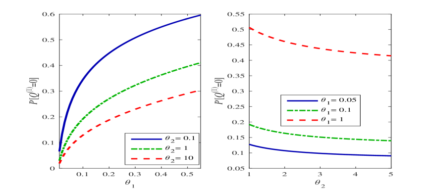
Figure 4: $P\left\{\mathcal{Q}^{\left(1\right)}=0\right\}$ vs $\theta_{1}$ and $\theta_{2}$

From Figure 5, it is seen that the stationary probability $P\left\{\mathcal{Q}^{\left(2\right)}=0\right\}$ decreases as $\theta_{1}$ increases, while it increases as $\theta_{2}$ increases.

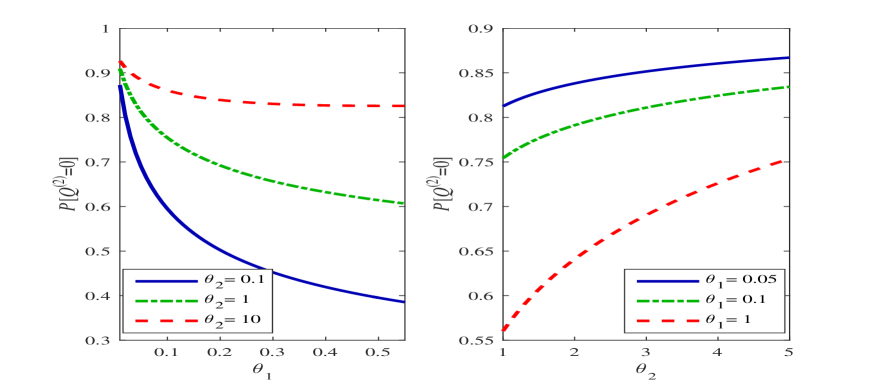
Figure 5: $P\left\{\mathcal{Q}^{\left(2\right)}=0\right\}$ vs $\theta_{1}$ and $\theta_{2}$

A coupling analysis: The two numerical results can be intuitively understood by means of the coupling method. As $\theta_{1}$ increases, more and more A-customers are quickly leaving the system due to their impatient behavior, thus $P\left\{\mathcal{Q}^{\left(1\right)}=0\right\}$ increases. On the other hand, as $\theta_{2}$ increases, more and more B-customers are quickly leaving the system so that the chance that an A-customer can match a B-customer will become smaller and smaller, hence this leads to the decrease of $P\left\{\mathcal{Q}^{\left(1\right)}=0\right\}$.

From Figure 6, we observed an interesting phenomenon: The stationary probability that there is neither A-customer nor B-customer, $P\left\{\mathcal{Q}=0\right\}$, increases as $\theta_{1}$ or $\theta_{2}$ increase.

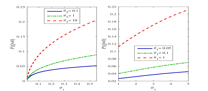
Figure 6: $P\left\{\mathcal{Q}=0\right\}$ vs $\theta_{1}$ and $\theta_{2}$

In what follows we discuss the average stationary queue lengths for the A-customers, the B-customers and the total system, respectively.

Figure 7 shows that the average stationary queue length $E\left[\mathcal{Q}^{\left(1\right)}\right]$ decreases as $\theta_{1}$ increases, while it increases as $\theta_{2}$ increases. From Figure 8, we observe that the average stationary queue length $E\left[\mathcal{Q}^{\left(2\right)}\right]$ increases as $\theta_{1}$ increases, while it decreases as $\theta_{2}$ increases.

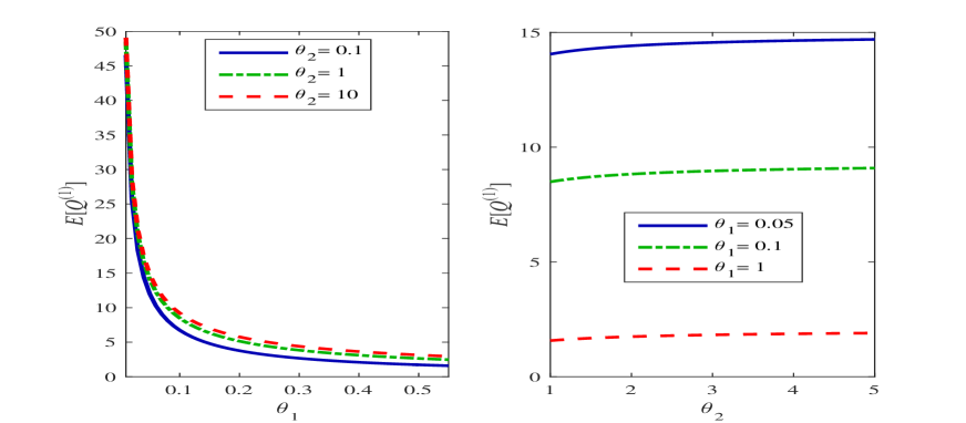
Figure 7: $E\left[\mathcal{Q}^{\left(1\right)}\right]$ vs $\theta_{1}$ and $\theta_{2}$

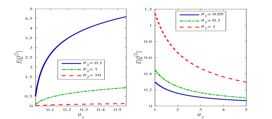
Figure 8: $E\left[\mathcal{Q}^{\left(2\right)}\right]$ vs $\theta_{1}$ and $\theta_{2}$

A coupling analysis: The two numerical results are intuitive. As $\theta_{1}$ increases, more and more A-customers are quickly leaving the system so that $E\left[\mathcal{Q}^{\left(1\right)}\right]$ decreases. On the other hand, as $\theta_{2}$ increases, more and more B-customers are quickly leaving the system so that the chance that an A-customer can match a B-customer will become smaller and smaller. Thus, $E\left[\mathcal{Q}^{\left(1\right)}\right]$ increases as $\theta_{2}$ increases.

From Figure 9, it is seen that the average stationary queue length $E\left[\mathcal{Q}\right]$ decreases as $\theta_{1}$ increases. But, $E\left[\mathcal{Q}\right]$ has a more consistent behavior as $\theta_{2}$ increases.

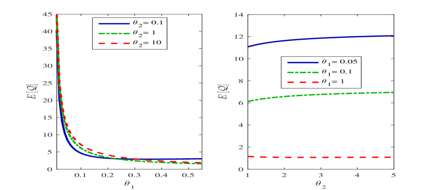
Figure 9: $E\left[\mathcal{Q}\right]$ vs $\theta_{1}$ and $\theta_{2}$

(b) The sojourn time

In this subsection, by using Algorithm three, we use some numerical examples to indicate how the average sojourn time $E\left[W_{A}\right]$ depends on the impatient rate $\theta_{1}$ and the number $k$ of A-customers in the double-ended queue.

For the two types of customers, we respectively take their MAPs with irreducible matrix representations as follows:

$$C_{1}=\left(\begin{array}[c]{cc}-10&0\\ 1&-1\end{array}\right),\text{ }D_{1}=\left(\begin{array}[c]{cc}9&1\\ 0&0\end{array}\right);$$

$$C_{2}=\left(\begin{array}[c]{cc}-5&1\\ 2&-7\end{array}\right),\text{ }D_{2}=\left(\begin{array}[c]{cc}0&4\\ 2&3\end{array}\right).$$

It is easy to compute that $\alpha_{1}=\left(1/2,1/2\right)$ and $\alpha_{2}=\left(4/9,5/9\right)$, hence their same stationary arrival rates are given by $\lambda_{1}=\alpha_{1}D_{1}\mathbf{e}=5$ and $\lambda_{2}=\alpha_{2}D_{2}\mathbf{e}=4\frac{5}{9}$.

Figure 10 indicates that when $\theta_{2}=0.1,1,10$, $E\left[W_{A}\right]$ decreases as $\theta_{1}$ increases for $\theta_{1}\in\left[0.01,0.55\right]$. Figure 11 shows that when $\theta_{1}=1,2,5$, $E\left[W_{A}^{\left(k\right)}\right]$ increases as $k$ increases for $k=5,6,\ldots,50$. As $\theta_{1}$ increases, the arriving A-customer can quickly leave the system due to her impatient behavior, thus $E\left[W_{A}\right]$ decreases. As $k$ increases, the total matching time length of the $k-1$ A-customer in front of this arriving A-customer will increase. This shows that $E\left[W_{A}^{\left(k\right)}\right]$ increases, as $k$ increases.

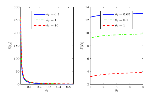
Figure 10: $E\left[W_{A}\right]$ vs $\theta_{1}$

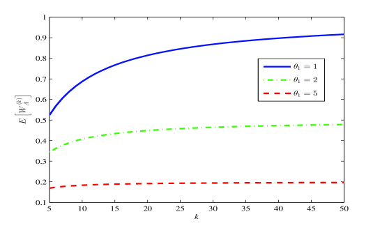
Figure 11: $E\left[W_{A}^{\left(k\right)}\right]$ vs $k$

Now, we consider another example with the two MAPs of order 4 (i.e., the order of the irreducible matrix representation is $4$), both of which have the same stationary arrival rates as that in the previous example, i.e., $\lambda_{1}=\alpha_{1}D_{1}\mathbf{e}=5$ and $\lambda_{2}=\alpha_{2}D_{2}\mathbf{e}=4\frac{5}{9}$. Also, the two MAPs of order 4 have the irreducible matrix representations as follows:

$$C_{1}=\left(\begin{array}[c]{cccc}-7&0&2&0\\ 2&-7&3&0\\ 0&0&-10&0\\ 2&1&2&-8\end{array}\right),\text{ }D_{1}=\left(\begin{array}[c]{cccc}0&5&0&0\\ 0&1&1&0\\ 0&0&2&8\\ 3&0&0&0\end{array}\right);$$

$$C_{2}=\left(\begin{array}[c]{cccc}-2&0&0&0\\ 0&-7&0&0\\ 0&0&-15&0\\ 1/2&0&5/2&-5\end{array}\right),\text{ }D_{2}=\left(\begin{array}[c]{cccc}0&2&0&0\\ 0&3&4&0\\ 3&0&2&10\\ 2&0&0&0\end{array}\right).$$

It is easy to check that $\alpha_{1}=\left(1/4,1/4,1/4,1/4\right)$ and $\alpha_{2}=\left(4/9,2/9,1/9,2/9\right)$. Hence we obtain that $\lambda_{1}=\alpha_{1}D_{1}\mathbf{e}=5$ and $\lambda_{2}=\alpha_{2}D_{2}\mathbf{e}=4\frac{5}{9}$.

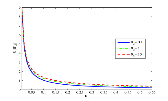
Figure 12: $E\left[W_{A}\right]$ vs $\theta_{1}$

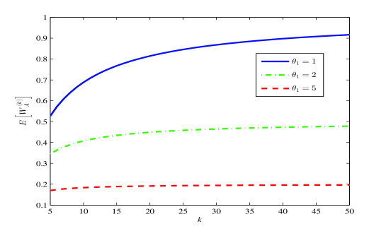
Figure 13: $E\left[W_{A}^{\left(k\right)}\right]$ vs $k$

It is observed from Figure 12 that when $\theta_{2}=0.1,1,10$, $E\left[W_{A}\right]$ decreases as $\theta_{1}$ increases for $\theta_{1}\in\left[0.01,0.55\right]$. Figure 13 shows that when $\theta_{1}=1,2,5$, $E\left[W_{A}^{\left(k\right)}\right]$ increases as $k$ increases for $k=5,6,\ldots,50$. Thus, it is easy to see that there are two identical changing trends of $E\left[W_{A}^{\left(k\right)}\right]$ through observing Figures 10 and 12, and Figures 11 and 13, respectively.

(c) Further numerical analysis

Now, we show that the above three algorithms developed in Section 6 are effective in numerical analysis of the double-ended queue when the two MAPs have different orders. To do this, we discuss three different cases: (1) The Poisson processes, (2) the MAP of order $2$, and (3) the MAP of order $4$. Also, it is seen from our numerical experiments that we can easily deal with the cases with MAPs of higher order.

We consider the double-ended queue from two groups of different impatient rates: $\left(\theta_{1},\theta_{2}\right)=\left(0.25,1\right)$, and $\left(\theta_{1},\theta_{2}\right)=\left(0.75,1\right)$, respectively. While for the arrival processes in two sides, we consider three different cases with the same stationary arrival rates: $\lambda_{1}=\alpha_{1}D_{1}\mathbf{e}=5$ and $\lambda_{2}=\alpha_{2}D_{2}\mathbf{e}=4\frac{5}{9}$. Further, we take the two arrival processes as follows:

(1) Two Poisson processes with arrival rates $\lambda_{1}=5$ and $\lambda_{2}=4\frac{5}{9}$, respectively.

(2) Two MAPs of order 2 whose irreducible matrix representations are given by

$$C_{1}=\left(\begin{array}[c]{cc}-10&0\\ 1&-1\end{array}\right),\text{ }D_{1}=\left(\begin{array}[c]{cc}9&1\\ 0&0\end{array}\right);$$

$$C_{2}=\left(\begin{array}[c]{cc}-5&1\\ 2&-7\end{array}\right),\text{ }D_{2}=\left(\begin{array}[c]{cc}0&4\\ 2&3\end{array}\right),$$

respectively.

(3) Two MAP of order 4 whose irreducible matrix representations are given by

$$C_{1}=\left(\begin{array}[c]{cccc}-7&0&2&0\\ 2&-7&3&0\\ 0&0&-10&0\\ 2&1&2&-8\end{array}\right),\text{ }D_{1}=\left(\begin{array}[c]{cccc}0&5&0&0\\ 0&1&1&0\\ 0&0&2&8\\ 3&0&0&0\end{array}\right);$$

$$C_{2}=\left(\begin{array}[c]{cccc}-2&0&0&0\\ 0&-7&0&0\\ 0&0&-15&0\\ 1/2&0&5/2&-5\end{array}\right),\text{ }D_{2}=\left(\begin{array}[c]{cccc}0&2&0&0\\ 0&3&4&0\\ 3&0&2&10\\ 2&0&0&0\end{array}\right),$$

respectively.

Based on the three different arrival processes, Table 1 provides a numerical comparison for the performance measures of the double-ended queue.

Table 1  Comparison of performance measures under different arrival processes
$\left(\theta_{1},\,\theta_{2}\right)$ Arrival Process $P\left\{\mathcal{Q}^{\left(1\right)}=0\right\}$ $P\left\{\mathcal{Q}^{\left(2\right)}=0\right\}$ $P\left\{\mathcal{Q}=0\right\}$ $E\left[\mathcal{Q}^{\left(1\right)}\right]$ $E\left[\mathcal{Q}^{\left(2\right)}\right]$ $E\left[\mathcal{Q}\right]$ $E\left[W_{A}\right]$ (0.25, 1) Poisson 0.2850 0.8174 0.1024 3.3181 0.3851 2.4429 0.5423 MAP of order 2 0.3119 0.6600 0.0526 4.1073 0.7565 2.6912 0.5995 MAP of order 4 0.2853 0.8068 0.0966 3.4584 0.4222 2.5357 0.5827 (0.75, 1) Poisson 0.4699 0.6989 0.1688 1.4392 0.6350 0.9542 0.2016 MAP of size 2 0.5103 0.5338 0.0861 1.6470 1.2327 1.2601 0.2038 MAP of size 4 0.4646 0.6890 0.1571 1.5095 0.6892 1.0149 0.2243

From Table 1, it is seen that the performance measures with two Poisson processes are close to that with two MAPs of order 4; while they are significantly different from that with two MAPs of order 2.

From the numerical computation in Table 1, it is seen that our three algorithms (by using the matrix-analytic method and the RG-factorizations), developed in Section 6, can effectively deal with the MAPs of higher orders in numerical analysis of the double-ended queue, for example, the MAP of order 10, the MAP of order 20, and so on.

In what follows we further give a numerical example to compare the results of this paper with that given by the multi-layer MMFF method given in Wu and He [70] and by the diffusion method given in Liu et al. [50]. We assume that the interarrival times of the arrival processes intwo sides are taken as follows:

Case one: The two exponential distributions with parameters $\lambda_{1}=1$ and $\lambda_{2}=2$, respectively.

Case two: The two Erlang distributions of order $2$ whose parameters are given by $2\lambda_{1}=2$ and $2\lambda_{2}=4$, respectively.

If the two interarrival times are exponential with parameter $\lambda_{1}=1$ and $\lambda_{2}=2$ respectively, then both of them correspond to the MAPs of order $1$, that is,

$$C_{1} =-1,\text{ }D_{1}=1;\text{ }$$

$$C_{2} =-2,\text{ }D_{2}=2\text{.}$$

If the two Erlang distributions of order $2$ whose parameters are given by $2\lambda_{1}=2$ and $2\lambda_{2}=4$ respectively, then both of them correspond to the MAPs of order $2$, that is,

$$C_{1}=\left(\begin{array}[c]{cc}-2&2\\ 0&-2\end{array}\right),\text{ }D_{1}=\left(\begin{array}[c]{cc}0&0\\ 2&0\end{array}\right);$$

$$C_{2}=\left(\begin{array}[c]{cc}-4&4\\ 0&-4\end{array}\right),\text{ }D_{2}=\left(\begin{array}[c]{cc}0&0\\ 4&0\end{array}\right).$$

Note that $\alpha_{1}=\alpha_{2}=\left(1/2,1/2\right)$, thus we obtain that $\lambda_{1}=\alpha_{1}D_{1}\mathbf{e}=1$ and $\lambda_{2}=\alpha_{2}D_{2}\mathbf{e}=2$.

Table 2  Numerical comparison of average stationary queue length difference $E\left[\mathcal{Q}^{\left(1\right)}\right]-E\left[\mathcal{Q}^{\left(2\right)}\right]$ among three different methods
Parameters Our bilateral QBD Multi-layer MMFF method of Wu and He (2021) Diffusion method of Liu et al. (2014) $\left(\lambda_{1},\,\lambda_{2}\right)\left(1,\,2\right)$ $\left(\theta_{1},\,\theta_{2}\right)$ $M=N=1000$ $M=N=2000$ Simulation Poisson Diffusion  1 Diffusion  2 Erlang(2) (1, 2) -0.4491 -0.4396 -0.4334 -0.4285 -0.3858 -0.4493 -0.5 ($4.81\%$) ($2.58\%$) ($1.13\%$) ($\pm 0.0018$) ($9.96\%$) ($4.87\%$) ($16.69\%$) Erlang(2) (0.1, 0.2) -5.1495 -5.0847 -5.0407 -4.9832 -4.9719 -4.9983 -5 ($3.34\%$) ($2.04\%$) ($1.15\%$) ($\pm 0.0015$) ($0.23\%$) ($0.30\%$) ($0.34\%$) Erlang(2) (0.01, 0.02) -50.8400 -50.8731 -50.4535 -50.089 -50 -50 -50 ($1.50\%$) ($1.57\%$) ($0.73\%$) ($\pm 0.1507$) ($0.18\%$) ($0.18\%$) ($0.18\%$) Exponential (1, 2) -0.3858 -0.4007 -0.3933 -0.3876 -0.3858 -0.3178 -0.5 ($0.46\%$) ($3.38\%$) ($1.46\%$) ($\pm 0.002$) ($0.46\%$) ($18\%$) ($29\%$) Exponential (0.1, 0.2) -4.9719 -5.0620 -5.0171 -4.9779 -4.9719 -4.9776 -5 ($0.12\%$) ($1.69\%$) ($0.79\%$) ($\pm 0.0157$) ($0.12\%$) ($0.01\%$) ($0.45\%$) Exponential (0.01, 0.02) -50 -50.8615 -50.4406 -49.9609 -50 -50 -50 ($0.08\%$) ($1.80\%$) ($0.96\%$) ($\pm 0.142$) ($0.08\%$) ($0.08\%$) ($0.08\%$)

In contrast with a simulation result, we define a relative error ratio of Method A as

$$x\%=\frac{100\left(\text{The numerical result given by Method A }-\text{ The simulation result}\right)}{\text{The simulation result}}\%\text{.}$$

From Columns $3$ to $9$ in Table 2, it is easy to see that the relative error ratios (in the brackets) of our bilateral QBD process are very close to that given by both the multi-layer MMFF method of Wu and He (2021) and the diffusion method of Liu et al. (2014). From such a comparison as well as the numerical computation of the well-known matrix-analytic method, our bilateral QBD process has two advantages: (a) It can easily provide a more detailed performance analysis of the double-ended queues, especially in the cases with MAP (non-Poisson) inputs. (b) Our bilateral QBD process can easily provide numerical computation of the double-ended queues with MAPs of higher order through using the matrix-analytic method and the RG-factorizations.

8 Concluding Remarks

In this paper, we study a block-structured double-ended queue with two MAP inputs and customers’ impatient behavior, and show that such a double-ended queue can be expressed as a new bilateral QBD process. Based on this finding, we provide a detailed analysis for the block-structured double-ended queue, including the system stability, the stationary queue length and the sojourn time. At the same time, we develop three effective algorithms for numerically computing performance measures of the block-structured double-ended queue, such as the probabilities of stationary queue lengths, the average stationary queue lengths, and the average sojourn time. Finally, we use some numerical examples to indicate how the performance measures are influenced by key system parameters. We believe that the methodology and results given in this paper can be applicable to deal with more general double-ended queues in practice, and further develop some effective algorithms for the purpose of many actual uses.

Along these lines, we will continue our future research on the following directions:

– Consider more general double-ended queues, for example, a double-ended queue with two BMAP inputs, a double-ended queue with a BMAP input and a renewal-process input, and a double-ended queue with matching batch size pair $(m,n)$.

– Develop more bilateral block-structured Markov processes, for example, bilateral Markov processes of GI/M/1 type, bilateral Markov processes of M/G/1 type, and so on.

– Develop effective algorithms for analyzing bilateral block-structured Markov processes and provide numerical analysis for more general matching issues in practice.

– Develop stochastic optimization and dynamic control, Markov decision processes and stochastic game theory in the study of double-ended queues. In this case, developing effective algorithms for dealing with optimal and control issues of the double-ended queues.

Appendix

This appendix provides the proofs of Theorems 1 and 4. Our purpose is to increase the readability of the main paper.

(a) Proof of Theorem 1

It is easy to see the irreducibility of the bilateral QBD process $Q$ through observing Figure 2, and using the two MAP inputs as well as the two exponential impatient times with $\left(\theta_{1},\theta_{2}\right)>0$.

Note that the bilateral QBD process $Q$ is positive recurrent if and only if the two unilateral QBD processes $Q_{A}$ and $Q_{B}$ are positive recurrent, thus it is key to find some necessary and sufficient conditions for the stability of the two unilateral QBD processes $Q_{A}$ and $Q_{B}$ by means of Neuts’ method (i.e., the mean drift technique).

For the QBD process $Q_{A}$, let $\mathbb{A}_{k}=A_{0}^{\left(k\right)}+A_{1}^{\left(k\right)}+A_{2}^{\left(k\right)}$. Then for $k\geq 1$ we obtain

$$\mathbb{A}_{k} =I\otimes D_{1}+C_{2}\oplus C_{1}-k\theta_{1}I+D_{2}\otimes I+k\theta_{1}I$$

$$=I\otimes D_{1}+C_{2}\oplus C_{1}+D_{2}\otimes I$$

$$=I\otimes D_{1}+I\otimes C_{1}+C_{2}\otimes I+D_{2}\otimes I$$

$$=I\otimes\left(C_{1}+D_{1}\right)+\left(C_{2}+D_{2}\right)\otimes I$$

$$=\left(C_{2}+D_{2}\right)\oplus\left(C_{1}+D_{1}\right),$$

which is independent of the positive integer $k\geq 1$. Obviously, $\mathbb{A}_{k}$ is the infinitesimal generator of the continuous-time Markov process with $m_{1}m_{2}$ states.

Note that $\alpha_{1}$ and $\alpha_{2}$ are the stationary probability vectors of the Markov processes $C_{1}+D_{1}$ and $C_{2}+D_{2}$, respectively. Thus, $\alpha_{1}\left(C_{1}+D_{1}\right)=\mathbf{0}$, $\alpha_{1}\mathbf{e}=1$; and $\alpha_{2}\left(C_{2}+D_{2}\right)=\mathbf{0}$, and $\alpha_{2}\mathbf{e}=1$. For each $k\geq 1$, we get

$$\left(\alpha_{2}\otimes\alpha_{1}\right)\mathbb{A}_{k} =\left(\alpha_{2}\otimes\alpha_{1}\right)\left[\left(C_{2}+D_{2}\right)\oplus\left(C_{1}+D_{1}\right)\right]$$

$$=\left(\alpha_{2}\otimes\alpha_{1}\right)\left[\left(C_{2}+D_{2}\right)\otimes I\right]+\left(\alpha_{2}\otimes\alpha_{1}\right)\left[I\otimes\left(C_{1}+D_{1}\right)\right]$$

$$=\left[\alpha_{2}\left(C_{2}+D_{2}\right)\right]\otimes\left(\alpha_{1}I\right)+\left(\alpha_{2}I\right)\otimes\left[\alpha_{1}\left(C_{1}+D_{1}\right)\right]$$

$$=\mathbf{0}$$

and

$$\left(\alpha_{2}\otimes\alpha_{1}\right)\left(\mathbf{e}\otimes\mathbf{e}\right)=\left(\alpha_{2}\mathbf{e}\right)\otimes\left(\alpha_{1}\mathbf{e}\right)=1.$$

Therefore, $\alpha_{2}\otimes\alpha_{1}$ is the stationary probability vector of the Markov process $\mathbb{A}_{k}$ for each $k\geq 1$.

Now, we compute the (upward and downward) mean drift rates of the QBD process $Q_{A}$. From Level $k$ to Level $k+1$, we obtain

$$\left(\alpha_{2}\otimes\alpha_{1}\right)A_{0}^{\left(k\right)}\mathbf{e} =\left(\alpha_{2}\otimes\alpha_{1}\right)\left(I\otimes D_{1}\right)\left(\mathbf{e}\otimes\mathbf{e}\right)$$

$$=\left(\alpha_{2}I\mathbf{e}\right)\otimes\left(\alpha_{1}D_{1}\mathbf{e}\right)=\lambda_{1}.$$

Similarly, from Level $k$ to Level $k-1$, we get

$$\text{\ }\left(\alpha_{2}\otimes\alpha_{1}\right)A_{2}^{\left(k\right)}\mathbf{e} =\left(\alpha_{2}\otimes\alpha_{1}\right)\left[D_{2}\otimes I+k\theta_{1}I\right]\mathbf{e}$$

$$=\left(\alpha_{2}\otimes\alpha_{1}\right)\left(D_{2}\otimes I\right)\mathbf{e+}\left(\alpha_{2}\otimes\alpha_{1}\right)k\theta_{1}I\mathbf{e}$$

$$=\lambda_{2}+k\theta_{1}.$$

Since $k$ is a positive integer and $\theta_{1}>0$, it is easy to check that if $k>\max\left\{1,\left(\lambda_{1}-\lambda_{2}\right)/\theta_{1}\right\}$, then $\left(\alpha_{2}\otimes\alpha_{1}\right)A_{0}^{\left(k\right)}\mathbf{e<}$ $\left(\alpha_{2}\otimes\alpha_{1}\right)A_{2}^{\left(k\right)}\mathbf{e}$. Therefore, the QBD process $Q_{A}$ must be positive recurrent due to the fact that the positive integer $k$ goes to infinity.

On the other hand, we can similarly discuss the stability of the QBD process $Q_{B}$. Let $\mathbb{B}_{k}=B_{0}^{\left(k\right)}+B_{1}^{\left(k\right)}+B_{2}^{\left(k\right)}$. Then we obtain

$$\mathbb{B}_{k} =D_{2}\otimes I+C_{2}\oplus C_{1}+k\theta_{2}I+I\otimes D_{1}-k\theta_{2}I$$

$$=\left(C_{2}+D_{2}\right)\oplus\left(C_{1}+D_{1}\right),$$

which is independent of the negative integer $k\leq-1$, and $\mathbb{B}_{k}$ is the infinitesimal generator of a continuous-time Markov process with $m_{1}m_{2}$ states.

For $k\leq-1$, we obtain

$$\left(\alpha_{2}\otimes\alpha_{1}\right)\mathbb{B}_{k} =\left(\alpha_{2}\otimes\alpha_{1}\right)\left[\left(C_{2}+D_{2}\right)\oplus\left(C_{1}+D_{1}\right)\right]$$

$$=\left(\alpha_{2}\otimes\alpha_{1}\right)\left[\left(C_{2}+D_{2}\right)\otimes I\right]+\left(\alpha_{2}\otimes\alpha_{1}\right)\left[I\otimes\left(C_{1}+D_{1}\right)\right]$$

$$=\left[\alpha_{2}\left(C_{2}+D_{2}\right)\right]\otimes\left(\alpha_{1}I\right)+\left(\alpha_{2}I\right)\otimes\left[\alpha_{1}\left(C_{1}+D_{1}\right)\right]$$

$$=\mathbf{0}$$

and

$$\left(\alpha_{2}\otimes\alpha_{1}\right)\left(\mathbf{e}\otimes\mathbf{e}\right)=\left(\alpha_{2}\mathbf{e}\right)\otimes\left(\alpha_{1}\mathbf{e}\right)=1.$$

Therefore, $\alpha_{2}\otimes\alpha_{1}$ is the stationary probability vector of the Markov process $\mathbb{B}_{k}$ for each $k\leq-1$.

Now, we compute the (upward and downward) mean drift rates of the QBD process $Q_{B}$. From Level $k$ to Level $k+1$, we yield

$$\text{\ }\left(\alpha_{2}\otimes\alpha_{1}\right)B_{2}^{\left(k\right)}\mathbf{e} =\left(\alpha_{2}\otimes\alpha_{1}\right)\left[\left(I\otimes D_{1}\right)-k\theta_{2}I\right]\mathbf{e}$$

$$=\left(\alpha_{2}I\mathbf{e}\right)\otimes\left(\alpha_{1}D_{1}\mathbf{e}\right)-\left(\alpha_{2}\otimes\alpha_{1}\right)k\theta_{2}I\mathbf{e}$$

$$=\lambda_{1}+\left(-k\right)\theta_{2}.$$

Similarly, from Level $k$ to Level $k-1$, we have

$$\left(\alpha_{2}\otimes\alpha_{1}\right)B_{0}^{\left(k\right)}\mathbf{e} =\left(\alpha_{2}\otimes\alpha_{1}\right)\left(D_{2}\otimes I\right)\left(\mathbf{e}\otimes\mathbf{e}\right)$$

$$=\left(\alpha_{2}D_{2}\mathbf{e}\right)\otimes\left(\alpha_{1}I\mathbf{e}\right)=\lambda_{2}.$$

Since $k$ is a negative integer and $\theta_{2}>0$, it is easy to check that if $k<\max\left\{-1,-\left(\lambda_{2}-\lambda_{1}\right)/\theta_{2}\right\}$, then $\left(\alpha_{2}\otimes\alpha_{1}\right)B_{0}^{\left(k\right)}\mathbf{e<}\left(\alpha_{2}\otimes\alpha_{1}\right)B_{2}^{\left(k\right)}\mathbf{e}$. Therefore, the QBD process $Q_{B}$ must be positive recurrent due to the fact that the negative integer $k$ goes to infinity.

Based on the above analysis, the two QBD processes $Q_{A}$ and $Q_{B}$ are all positive recurrent, so that the bilateral QBD process $Q$ is irreducible and positive recurrent. Therefore, the block-structured double-ended queue is stable. This completes the proof. $\blacksquare$

(b) Proof of Theorem 4

The proof is easy through checking that $\pi$ satisfies the system of linear equations $\pi Q=\mathbf{0}$ and $\pi\mathbf{e}=1$. To this end, we consider the following three different cases:

Case one: $k\geq 2$. In this case, we need to check that

$$\pi_{k-1}A_{0}^{\left(k-1\right)}+\pi_{k}A_{1}^{\left(k\right)}+\pi_{k+1}A_{2}^{\left(k+1\right)}=0.$$ (21)

Since $\pi_{k-1}=c\widetilde{\pi}_{k-1}=c\widetilde{\pi}_{1}R_{1}R_{2}\cdots R_{k-2},\pi_{k}=c\widetilde{\pi}_{k}=c\widetilde{\pi}_{1}R_{1}R_{2}\cdots R_{k-1}$ and $\pi_{k+1}=c\widetilde{\pi}_{k+1}=c\widetilde{\pi}_{1}R_{1}R_{2}\cdots R_{k}$, we obtain

$$\text{ \ \ }\pi_{k-1}A_{0}^{\left(k-1\right)}+\pi_{k}A_{1}^{\left(k\right)}+\pi_{k+1}A_{2}^{\left(k+1\right)}$$

$$=c\widetilde{\pi}_{1}R_{1}R_{2}\cdots R_{k-2}A_{0}^{\left(k-1\right)}+c\widetilde{\pi}_{1}R_{1}R_{2}\cdots R_{k-1}A_{1}^{\left(k\right)}+c\widetilde{\pi}_{1}R_{1}R_{2}\cdots R_{k}A_{2}^{\left(k+1\right)}$$

$$=c\widetilde{\pi}_{1}R_{1}R_{2}\cdots R_{k-2}\left(A_{0}^{\left(k-1\right)}+R_{k-1}A_{1}^{\left(k\right)}+R_{k-1}R_{k}A_{2}^{\left(k+1\right)}\right)=0$$

by means of (3).

Case two: $k\leq-2$. In this case, we need to check that

$$\pi_{k+1}B_{0}^{\left(k+1\right)}+\pi_{k}B_{1}^{\left(k\right)}+\pi_{k-1}B_{2}^{\left(k-1\right)}=0.$$ (22)

Note that $\pi_{k+1}=c\widetilde{\pi}_{k+1}=c\widetilde{\pi}_{-1}\mathbb{R}_{-1}\mathbb{R}_{-2}\cdots\mathbb{R}_{k+2},\pi_{k}=c\widetilde{\pi}_{k}=c\widetilde{\pi}_{-1}\mathbb{R}_{-1}\mathbb{R}_{-2}\cdots\mathbb{R}_{k+1}$ and $\pi_{k-1}=c\widetilde{\pi}_{k-1}=c\widetilde{\pi}_{-1}\mathbb{R}_{-1}\mathbb{R}_{-2}\cdots\mathbb{R}_{k}$, we have

$$\text{ \ \ }\pi_{k+1}B_{0}^{\left(k+1\right)}+\pi_{k}B_{1}^{\left(k\right)}+\pi_{k-1}B_{2}^{\left(k-1\right)}$$

$$=c\widetilde{\pi}_{-1}\mathbb{R}_{-1}\mathbb{R}_{-2}\cdots\mathbb{R}_{k+2}B_{0}^{\left(k+1\right)}+c\widetilde{\pi}_{-1}\mathbb{R}_{-1}\mathbb{R}_{-2}\cdots\mathbb{R}_{k+1}B_{1}^{\left(k\right)}+c\widetilde{\pi}_{-1}\mathbb{R}_{-1}\mathbb{R}_{-2}\cdots\mathbb{R}_{k}B_{2}^{\left(k-1\right)}$$

$$=c\widetilde{\pi}_{-1}\mathbb{R}_{-1}\mathbb{R}_{-2}\cdots\mathbb{R}_{k+2}\left(B_{0}^{\left(k+1\right)}+\mathbb{R}_{k+1}B_{1}^{\left(k\right)}+\mathbb{R}_{k+1}\mathbb{R}_{k}B_{2}^{\left(k-1\right)}\right)=0$$

in terms of (7).

Case three: $k=1,$ $0,$ $-1.$ In this case, we can check that

$$\left\{\begin{array}[c]{l}\pi_{0}A_{0}^{\left(0\right)}+\pi_{1}A_{1}^{\left(1\right)}+\pi_{2}A_{2}^{\left(2\right)}=0,\\ \pi_{-1}B_{2}^{\left(-1\right)}+\pi_{0}\left(B_{1}^{\left(0\right)}+A_{1}^{\left(0\right)}\right)+\pi_{1}A_{2}^{\left(1\right)}=0,\\ \pi_{-2}B_{2}^{\left(-2\right)}+\pi_{-1}B_{1}^{\left(-1\right)}+\pi_{0}B_{0}^{\left(0\right)}=0.\end{array}\right.$$ (23)

by means of $\pi_{0}=c\widetilde{\pi}_{0},\pi_{1}=c\widetilde{\pi}_{1},\pi_{2}=c\widetilde{\pi}_{2}=c\widetilde{\pi}_{1}R_{1},\pi_{-1}=c\widetilde{\pi}_{-1}$ and $\pi_{-2}=c\widetilde{\pi}_{-2}=c\widetilde{\pi}_{-1}\mathbb{R}_{-1}$.

Let $\mathbf{Z}$ be the set of all integers, i.e., $\mathbf{Z}=\left\{\ldots,-2,-1,0,1,2,\ldots\right\}$. Note that $\pi\mathbf{e}=1$, we compute

$$\sum_{k\in\mathbf{Z}}\pi_{k}\mathbf{e}=1$$ (24)

by means of $\pi_{k}=c\widetilde{\pi}_{k}=c\widetilde{\pi}_{1}R_{1}R_{2}\cdots R_{k-1}$ for $k\geq 2,\pi_{1}=c\widetilde{\pi}_{1},\pi_{0}=c\widetilde{\pi}_{0},\pi_{-1}=c\widetilde{\pi}_{-1}$ and $\pi_{k}=c\widetilde{\pi}_{k}=c\widetilde{\pi}_{-1}\mathbb{R}_{-1}\mathbb{R}_{-2}\cdots\mathbb{R}_{k+1}$ for $k\leq-2$. Thus we have

$$1 =\sum_{k\in\mathbf{Z}}\pi_{k}\mathbf{e}=\sum_{k\leq-2}\pi_{k}\mathbf{e+}\pi_{-1}\mathbf{e+}\pi_{0}\mathbf{e+}\pi_{1}\mathbf{e+}\sum_{k=2}^{\infty}\pi_{k}\mathbf{e}$$

$$=\sum_{k\leq-2}c\widetilde{\pi}_{-1}\mathbb{R}_{-1}\mathbb{R}_{-2}\cdots\mathbb{R}_{k+1}\mathbf{e+}c\widetilde{\pi}_{-1}\mathbf{e+}c\widetilde{\pi}_{0}\mathbf{e+}c\widetilde{\pi}_{1}\mathbf{e+}\sum\limits_{k=2}^{\infty}c\widetilde{\pi}_{1}R_{1}R_{2}\cdots R_{k-1}\mathbf{e}$$

$$=c\left(\sum_{k\leq-2}\widetilde{\pi}_{-1}\mathbb{R}_{-1}\mathbb{R}_{-2}\cdots\mathbb{R}_{k+1}\mathbf{e}+\widetilde{\pi}_{-1}\mathbf{e}+\widetilde{\pi}_{0}\mathbf{e}+\widetilde{\pi}_{1}\mathbf{e}+\sum\limits_{k=2}^{\infty}\widetilde{\pi}_{1}R_{1}R_{2}\cdots R_{k-1}\mathbf{e}\right),$$

which gives the positive constant $c$ in (12). This completes the proof. $\blacksquare$

References

- [1] Afèche, P., Diamant, A., Milner, J., 2014. Double-sided batch queues with abandonment: Modeling crossing networks. Operations Research 62(5), 1179–1201.
- [2] Artalejo, J.R., Gómez-Corral, A., 2008. Retrial Queueing Systems: A Computational Approach. Springer
- [3] Axsäer, S., 2015. Inventory Control. Springer.
- [4] Azevedo, E.M., Weyl, E.G., 2016. Matching markets in the digital age. Science 352(6289), 1056–1057.
- [5] Baik, H., Sherali, H.D., Trani, A.A., 2002. Time-dependent network assignment strategy for taxiway routing at airports. Transportation research record 1788(1), 70–75.
- [6] Banerjee, S., Johari, R., 2019. Ride sharing. In: Sharing Economy. Springer, pp. 73–97.
- [7] Benjaafar, S., Hu, M., 2019. Operations management in the age of the sharing economy: What is old and what is new? Manufacturing and Service Operations Management 22(1), 93–101.
- [8] Bhat, U.N., 1970. A controlled transportation queueing process. Management Science 16(7), 446–452.
- [9] Boxma, O.J., David, I., Perry, D., Stadje, W., 2011. A new look at organ transplantation models and double matching queues. Probability in the Engineering and Informational Sciences 25(2), 135–155.
- [10] Braverman, A., Dai, J.G., Liu, X., Ying, L., 2019. Empty-car routing in ridesharing systems. Operations Research 67(5), 1437–1452.
- [11] Bright, L., Taylor, P.G., 1995. Calculating the equilibrium distribution in level dependent quasi-birth-and-death processes. Stochastic Models 11(3), 497–525.
- [12] Bright, L., Taylor, P.G., 1997. Equilibrium distributions for level-dependent quasi-birth-and-death processes. In: Matrix-Analytic Methods in Stochastic Models. Marcel Dekker, pp. 359–375.
- [13] Browne, J.J., Kelly, J.J., Le Bourgeois, P., 1970. Maximum inventories in baggage claim: a double ended queuing system. Transportation Science 4(1), 64–78.
- [14] Büke, B., Chen, H., 2015. Stabilizing policies for probabilistic matching systems. Queueing Systems 80(1-2), 35–69.
- [15] Büke. B., Chen, H., 2017. Fluid and diffusion approximations of probabilistic matching systems. Queueing Systems 86(1-2), 1–33.
- [16] Chakravarthy, S.R., 2001. The batch Markovian arrival process: A review and future work. In: Advances in probability theory and stochastic processes, Vol. 1. Notable Publications Inc NJ, pp. 21–49.
- [17] Cheng, M., 2016. Sharing economy: A review and agenda for future research. International Journal of Hospitality Management 57(1), 60–70.
- [18] Conolly, B.W., Parthasarathy, P.R., Selvaraju, N., 2002. Double-ended queues with impatience. Computers & Operations Research 29(14), 2053–2072.
- [19] Cordeiro, J.D., Kharoufeh, J.P., 2010. Batch markovian arrival processes (BMAP). In: Wiley Encyclopedia of Operations Research and Management Science. https://doi.org/10.1002/9780470400531.eorms0096.
- [20] Di Crescenzo, A., Giorno, V., Kumar, B.K., Nobile, A.G., 2012. A double-ended queue with catastrophes and repairs, and a jump-diffusion approximation. Methodology and Computing in Applied Probability 14(4), 937–954.
- [21] Di Crescenzo, A., Giorno, V., Kumar, B.K., Nobile, A.G., 2018. A time-non-homogeneous double-ended queue with failures and repairs and its continuous approximation. Mathematics 6(81), 1–23.
- [22] Diamant, A., Baron, O., 2019. Double-sided matching queues: Priority and impatient customers. Operations Research Letters 47(3), 219–224.
- [23] Dobbie, J.M., 1961. Letter to the editor—a doubled-ended queuing problem of Kendall. Operations Research 9(5), 755–757.
- [24] Duenyas, I., Keblis, M.F., Pollock, S.M., 1997. Dynamic type matching. Management Science 43(6), 751–763.
- [25] Elalouf, A., Perlman, Y., Yechiali, U., 2018. A double-ended queueing model for dynamic allocation of live organs based on a best-fit criterion. Applied Mathematical Modelling 60, 179–191.
- [26] Giveen, S.M., 1961. A taxicab problem considered as a double-ended queue. Operations Research 9, B44.
- [27] Giveen, S.M., 1963. A taxicab problem with time-dependent arrival rates. SIAM Review 5(2), 119–127.
- [28] Gurvich, I., Ward, A., 2014. On the dynamic control of matching queues. Stochastic Systems 4(2), 479–523.
- [29] Hlynka, M., Sheahan, J.N., 1987. Controlling rates in a double queue. Naval Research Logistics 34(4), 569–577.
- [30] Hopp, W.J., Simon, J.T., 1989. Bounds and heuristics for assembly-like queues. Queueing systems 4(2), 137–155.
- [31] Hu, M., Zhou, Y., 2015. Dynamic type matching. Working Paper No. 2592622, Rotman School of Management, University of Toronto, Available at SSRN: https://ssrn.com/abstract=2592622.
- [32] Jain, H.C., 1962. A double-ended queuing system. Defence Science Journal 12(4), 327–332.
- [33] Jain, M., 1995. A sample path analysis for double ended queue with time dependent rates. International J. Mgmt. & Syst. 11(1), 125–130.
- [34] Jain, M., 2000. G/G/1 double ended queue: diffusion approximation. Journal of Statistics and Management Systems 3(2), 193–203.
- [35] Kashyap, B.R.K., 1965. A double-ended queueing system with limited waiting space. Proc. Nat. Inst. Sci. India 31(6), 559–570.
- [36] Kashyap, B.R.K., 1966. The double-ended queue with bulk service and limited waiting space. Operations Research 14(5), 822–834.
- [37] Kashyap, B.R.K., 1967. Further results for the double ended queue. Metrika 11(1), 168–186.
- [38] Kendall, D.G., 1951. Some problems in the theory of queues. Journal of the Royal Statistical Society (Series B) 13(2), 151–185.
- [39] Kim, W.K., Yoon, K.P., Mendoza, G., Sedaghat, M., 2010. Simulation model for extended double-ended queueing. Computers & Industrial Engineering 59(2), 209–219.
- [40] Latouche, G., 1981. Queues with paired customers. Journal of Applied Probability 18(3), 684–696.
- [41] Lee, C., Liu, X., Liu, Y., Zhang, L., 2021. Optimal control of a time-varying double-ended production queueing model. Stochastic Systems 11(2), 140–173.
- [42] Li, Q.L., 2010. Constructive Computation in Stochastic Models with Applications: The RG-Factorizations. Springer.
- [43] Li, Q.L., Cao, J., 1996. Equilibrium behavior of the matched queueing system. In: Proceedings of the 2nd International Symposium on Operations Research and Its Applications. World Publishing Corporation, pp. 487–499.
- [44] Li, Q.L., Cao, J., 2004. Two types of RG-factorizations of quasi-birth-and-death processes and their applications to stochastic integral functionals. Stochastic Models 20(3), 299–340.
- [45] Li, Q.L., Liu, L., 2004. An algorithmic approach for sensitivity analysis of perturbed quasi-birth-and-death processes. Queueing System 48(3-4), 365–397.
- [46] Li, Q.L., Zhao, Y.Q., 2004. The RG-factorizations in block-structured Markov renewal processes. In: Observation, Theory And Modeling Of Atmospheric Variability. World Scientific, pp. 545–568.
- [47] Liu, H.L., Li, Q.L., Zhang, C., 2020. Matched queues with matching batch pair . arXiv preprint arXiv:2009.02742, pp. 1–38.
- [48] Liu, H.L., Li, Q.L., Wu, X., Zhang, C., 2021. Two basic queueing models of service platforms in digital sharing economy. arXiv preprint arXiv:2108.02852, pp. 1–35.
- [49] Liu, X., 2019. Diffusion approximations for double-ended queues with reneging in heavy traffic. Queueing Systems 91(1-2), 49–87.
- [50] Liu, X., Gong, Q., Kulkarni, V.G., 2014. Diffusion models for double-ended queues with renewal arrival processes. Stochastic Systems 5(1), 1–61.
- [51] Lucantoni, D.M., 1991. New results on the single server queue with a batch Markovian arrival process. Stochastic Models 7(1), 1–46.
- [52] Narayana, S., Neuts, M.F., 1992. The first two moment matrices of the counts for the Markovian arrival process. Communications in statistics. Stochastic Models 8(3), 459–477.
- [53] Neuts, M.F., 1979. A versatile Markovian point process. Journal of Applied Probility 16(4), 764–79.
- [54] Neuts, M.F., 1981. Matrix-Geometric Solutions in Stochastic Models: An Algorithmic Approach. Johns Hopkins University Press.
- [55] Neuts, M.F., 1989. Structural Stochastic Matrices of M/G/1 type and their applications. Marcel Dekker.
- [56] Pandey, M.K., Gangeshwer, D.K., 2018. Applications of the diffusion Approximation to hospital sector using G∞/GM/1 double ended queue model. Journal of Computer and Mathematical Sciences 9(4), 302–308.
- [57] Parthasarathy, P.R., Selvaraju, N., Manimaran, G., 1999. A paired queueing system arising in multimedia synchronization. Mathematical and Computer Modelling 30(11-12), 133–140.
- [58] Porteus, E.L., 1990. Stochastic inventory theory. In: Handbooks in Operations Research and Management Science, Vol. 2. North-Holland, pp. 605–652.
- [59] Ramachandran, S., Delen, D., 2005. Performance analysis of a kitting process in stochastic assembly systems. Computers & Operations Research 32(3), 449–463.
- [60] Ramaswami, V., Taylor, P.G., 1996. Some properties of the rate perators in level dependent quasi-birth-and-death processes with countable number of phases. Stochas tic Models, 12(1), 143-164.
- [61] Sasieni, M.W., 1961. Double queues and impatient customers with an application to inventory theory. Operations Research 9(6), 771–781.
- [62] Sharma, O.P., Nair, N.S.K., 1991. Transient behaviour of a double ended Markovian queue. Stochastic Analysis and Applications 9(1), 71–83.
- [63] Shi, Y., Lian, Z., 2016. Optimization and strategic behavior in a passenger–taxi service system. European Journal of Operational Research 249(3), 1024–1032.
- [64] Som, P., Wilhelm, W.E., Disney, R.L., 1994. Kitting process in a stochastic assembly system. Queueing Systems 17(3-4), 471–490.
- [65] Stanford, D.A., Lee, J.M., Chandok, N., McAlister, V., 2014. A queuing model to address waiting time inconsistency in solid-organ transplantation. Operations Research for Health Care 3(1), 40–45.
- [66] Steinmetz, R., 1990. Synchronization properties in multimedia systems. IEEE Journal on selected areas in communications, 8(3) 401–412.
- [67] Sutherland, W., Jarrahi, M.H., 2018. The sharing economy and digital platforms: A review and research agenda. International Journal of Information Management 43, 328–341.
- [68] Takahashi, M., Ōsawa, H., Fujisawa, T., 2000. On a synchronization queue with two finite buffers. Queueing Systems 36(1-3), 107–123.
- [69] Takahashi, M., Takahashi, Y.T., 2000. Synchronization queue with two MAP inputs and finite buffers. In: Proceedings of the Third International Conference on Matrix Analytical Methods in Stochastic Models, pp. 375–390.
- [70] Wu, H., He, Q.M., 2020. Double-sided queues with marked Markovian arrival processes and abandonment. Stochastic Models 37(1), 23–58.
- [71] Xu, G.H., He, Q.M., 1993. Matched queueing system . Acta Mathematicae Applicatae Sinica 9(2), 104–114.
- [72] Xu, G.H., He, Q.M., 1993. The matched queueing system . Acta Mathematicae Applicatae Sinica 10(1), 34–47.
- [73] Xu, G.H., He, Q.M., Liu, X.S., 1990. The matched queueing system with a double input. Acta Mathematicae Applicatae Sinica 13(1), 40–48. (in Chinese)
- [74] Xu, G.H., He, Q.M., Liu, X.S., 1993. Matched queueing systems with a double input. Acta Mathematicae Applicatae Sinica 9(1), 50–62.
- [75] Yuan, X.M., 1992. Stationary behavior of the matched queueing system with double input. Journal of Graduate school, Academia Sinica 9(1), 1–10. (in Chinese)
- [76] Zenios, S.A., 1999. Modeling the transplant waiting list: A queueing model with reneging. Queueing systems 31(3-4), 239–251.
- [77] Zhang, W., Honnappa, H., Ukkusuri, S.V., 2019. Modeling urban taxi services with e-hailings: A queueing network approach. Transportation Research Part C: Emerging Technologies 113, 332–349.