The calculation of the neutrinoless double-$\beta$ decay matrix element within the realistic shell model

Abstract

We approach the calculation of the nuclear matrix element of the neutrinoless double-$\beta$ decay process, considering the light-neutrino-exchange channel, by way of the realistic shell model. To this end, we start from a realistic nucleon-nucleon potential and then derive the effective shell-model Hamiltonian and $0\nu\beta\beta$-decay operator within the many-body perturbation theory. We focus on investigating the perturbative properties of the effective shell-model operator of such a decay process, aiming to establish the degree of reliability of our predictions. The contributions of the so-called short-range correlations and of the correction of Pauli-principle violations to the effective shell-model operator, the latter introduced in many-valence nucleon systems, are also taken into account. The subjects of our study are a few candidates to the $0\nu\beta\beta$-decay detection, in a mass interval ranging from $A=48$ up to $A=136$, whose spin- and spin-isospin-dependent decay properties we have studied in previous works. Our results evidence that the effect of the renormalization of the $0\nu\beta\beta$-beta decay operator on the values of the nuclear matrix elements is less relevant than what we have obtained in previous studies of the effective single-body GT transitions operating also in the two neutrinos double-beta decay

I Introduction

The search for evidence of the neutrinoless double-$\beta$ decay ($0\nu\beta\beta$) is at present one of the major goal in experimental physics, because of its implications in our understanding of both the limits of Standard Model and the intrinsic nature of the neutrino Avignone et al. (2008); Dell’Oro et al. (2016); Henning (2016).

Double-$\beta$ decay is a second-order electroweak process and the rarest among the nuclear transitions. As is well known, the $\beta$-decay with the emission of two neutrinos ($2\nu\beta\beta$) occurs with half-lives that exceed $10^{18}$ yr, and, at present, the strongest limits on $0\nu\beta\beta$ decay have been set as $>0.9\times 10^{26}$ yr for ⁷⁶Ge decay by GERDA experiment Agostini et al. (2019), $>4\times 10^{24}$ yr for ¹³⁰Te decay by CUORE experiment Alfonso et al. (2015), and $>1.07\times 10^{26}$ yr for ¹³⁶Xe decay by KamLAND-ZEN collaboration Gando et al. (2016).

The detection of $0\nu\beta\beta$ decay - a process that requires the violation of the conservation of the lepton number - would pave the way to a physics whose mechanisms should lie beyond the Standard Model. It would reveal the nature of the massive neutrino as a Majorana rather than a Dirac particle, being a spin-$\frac{1}{2}$ particle which coincides with its anti-particle. Such a feature may provide insight into the matter-antimatter asymmetry in the Universe within the framework of CP violation effects due to the see-saw and leptogenesis mechanisms Buchmüller et al. (2005).

The half-life of the $0\nu\beta\beta$ decay may be expressed as

$$\left[T^{0\nu}_{1/2}\right]^{-1}=G^{0\nu}\left|M^{0\nu}\right|^{2}\left|f(m_{i},U_{ei})\right|^{2}~{},$$ (1)

where $G^{0\nu}$ is the so-called phase-space factor (or kinematic factor) Kotila and Iachello (2012, 2013), $M^{0\nu}$ is the nuclear matrix element (NME) directly related to the wave functions of the parent and grand-daughter nuclei, and $f(m_{i},U_{ei})$ accounts for the physics beyond the standard model through the neutrino masses $m_{i}$ and their mixing matrix elements $U_{ei}$. The explicit form of $f(m_{i},U_{ei})$ depends on the adopted model of $0\nu\beta\beta$ decay (light- and/or heavy neutrino exchange, Majoron exchange, …).

In particular, within the mechanisms of light-neutrino exchange, $f(m_{i},U_{ei})$ has the following expression:

$$f(m_{i},U_{ei})=g_{A}^{2}\frac{\langle m_{\nu}\rangle}{m_{e}}$$

where $g_{A}$ is the axial coupling constant, $m_{e}$ is the electron mass, and $\langle m_{\nu}\rangle=\sum_{i}(U_{ei})^{2}m_{i}$ is the effective neutrino mass. The above expression and the one in (1) evidence the pivotal role played by the calculation of the NME.

In fact, a reliable estimate of its value provides important information about some crucial issues, since the neutrino effective mass can be expressed in terms of $M^{0\nu}$, of the half-life $T^{0\nu}_{1/2}$, and the so-called nuclear structure factor $F_{N}=G^{0\nu}\left|M^{0\nu}\right|^{2}g_{A}^{4}$, as $\langle m_{\nu}\rangle=m_{e}\left[F_{N}T^{0\nu}_{1/2}\right]^{-1/2}$. Moreover, combining the calculated nuclear structure factor with neutrino mixing parameters Tanabashi et al. (2018) and limits on $\langle m_{\nu}\rangle$ from current experiments, one may extract an estimation of the half-life an experiment should measure in order to be sensitive to a particular value of the neutrino effective mass Avignone et al. (2008). All the above considerations evidence that reliable calculations of $M^{0\nu}$ are of paramount importance, and, currently, various nuclear structure models are employed to study this process.

It should be noted that currently ab initio calculations may be carried out only for light nuclei Pastore et al. (2018), but the parameters that locate the best candidates of experimental interest - $Q$-value and phase-space factor of the decay, and the isotopic abundance of the parent nucleus - point to the region of medium- and heavy-mass nuclei. This is why the nuclear structure models which are mostly employed to study the $0\nu\beta\beta$ decay of nuclei of experimental interest are the Interacting Boson Model (IBM) Barea and Iachello (2009); Barea et al. (2012, 2013), the Quasiparticle Random-Phase Approximation (QRPA) Šimkovic et al. (2009); Fang et al. (2011); Faessler et al. (2012), Energy Density Functional methods Rodríguez and Martínez-Pinedo (2010), the Covariant Density Functional Theory Song et al. (2014); Yao et al. (2015); Song et al. (2017), the Generator-Coordinate Method (GCM) Jiao et al. (2017); Yao et al. (2018); Jiao et al. (2018); Jiao and Johnson (2019), and the Shell Model (SM) Menéndez et al. (2009a, b); Horoi and Brown (2013); Neacsu and Horoi (2015); Brown et al. (2015).

Actually, for all these calculations the truncation of the full Hilbert space is mandatory to diagonalize the nuclear Hamiltonian, and the renormalization of the effective Hamiltonian $H_{\rm eff}$  is generally performed fitting the parameters which characterize each model, and that are associated with the degrees of freedom of the reduced model space, to some spectroscopic properties of the nuclei under investigation. As a matter of fact, the determination of the model parameters is carried out taking into account the specific abilities of the different models, leading to a spread of the results of the calculation of $M^{0\nu}$ with different approaches, which agree within a factor $\sim 2\div 3$ (see, for example, Fig. 5 in Ref. Engel and Menéndez (2017) and references therein).

Aside from the renormalization of the nuclear Hamiltonian, whenever transition properties are calculated using wave functions obtained diagonalizing $H_{\rm eff}$, the free constants that appear in the definition of the decay operators - proton and neutron electric charges, spin and orbital gyromagnetic factors, etc. - need also to be modified to account for the degrees of freedom that do not appear explicitly because of the truncation of the full Hilbert space, a procedure that is also performed by fitting them to reproduce observables.

This leads to the well-known problem of quenching the free value of the axial coupling constant $g_{A}^{free}=1.2723$ Tanabashi et al. (2018) via a quenching factor $q$ Towner (1987), whose choice depends on the nuclear structure model, the dimensions of the reduced Hilbert space, and the mass of the nuclei under investigation Suhonen (2017a). We point out that both the renormalization of many-body correlations and the corrections due to the subnucleonic structure of the nucleons Park et al. (1993); Pastore et al. (2009); Piarulli et al. (2013); Baroni et al. (2016) are needed to handle the issue of quenching $g_{A}$, whose $q$ value is commonly determined fitting experimental data from Gamow-Teller (GT) transitions.

In this work, we will tackle the problem to calculate the $0\nu\beta\beta$-decay NME, in the light-neutrino-exchange channel, within the framework of the realistic shell model (RSM) Coraggio et al. (2009), that is the effective shell-model Hamiltonian $H_{\rm eff}$  and decay operators are consistently derived starting from a realistic nucleon-nucleon ($NN$) potential $V_{NN}$. This can be achieved by way of many-body perturbation theory Kuo et al. (1995); Hjorth-Jensen et al. (1995); Suzuki and Okamoto (1995); Coraggio et al. (2012), in order to construct single-particle (SP) energies, two-body matrix elements of the residual interaction (TBME), and two-body matrix elements of the effective $0\nu\beta\beta$-decay operator ($O^{0\nu}_{\rm eff}$) within a microscopic approach.

Our input $V_{NN}$ is the high-precision CD-Bonn $NN$ potential Machleidt (2001), whose repulsive high-momentum components are smoothed out using the $V_{{\rm low}\mbox{-}k}$ approach Bogner et al. (2002). The $V_{{\rm low}\mbox{-}k}$ procedure provides a consistent treatment of the so-called short-range correlations, which need to be included since the basis that is employed for the perturbative expansion consists of uncorrelated wave functions that do not vanish in the short range, the latter corresponding to the region of the strong-repulsive components of $V_{NN}$ Bethe (1971); Kortelainen et al. (2007).

We have pursued the approach of RSM already to calculate the $2\nu\beta\beta$  NME ($M^{2\nu}$) in Refs. Coraggio et al. (2017); Coraggio et al. (2019a) for ⁴⁸Ca, ⁷⁶Ge, ⁸²Se, ¹³⁰Te, and ¹³⁶Xe. In the same works a study of the spectroscopy of these nuclei, focussing in particular on spin-dependent decays, and of their GT-strength distributions has been also reported.

It should be mentioned that similar SM calculations of $M^{0\nu}$ have been performed in Refs. Wu et al. (1985); Song et al. (1991); Holt and Engel (2013).

Calculations of $M^{0\nu}$ for ⁴⁸Ca decay in Refs. Wu et al. (1985); Song et al. (1991) are based on a consistent treatement of the short-range correlations in terms of the defect wave functions Bethe (1971) derived from the calculation of the reaction matrix $G$ from Paris Lacombe et al. (1980) and Reid Reid (1968) $NN$ potentials. The $G$-matrix vertices appear also in the perturbative expansion of $H_{\rm eff}$  and $O^{0\nu}_{\rm eff}$, which is arrested at second order.

The authors in Ref. Holt and Engel (2013) focus their attention on $0\nu\beta\beta$ decay of ⁷⁶Ge and ⁸²Se, and start from a chiral N³LO $NN$ potential Entem and Machleidt (2002) renormalized through the $V_{{\rm low}\mbox{-}k}$ technique. They expand $O^{0\nu}_{\rm eff}$ up to third order in perturbation theory, and include the effects of high-momentum (short-range) correlations via an effective Jastrow function that has been fit to the results of Brueckner-theory calculations Šimkovic et al. (2009). The wave functions of parent and grand-daughter nuclei have been calculated using two different phenomenological SM $H_{\rm eff}$s  from Refs. Horoi (2013); Menéndez et al. (2009b) for ⁷⁶Ge and ⁸²Se decays, respectively.

In Section II details about the derivation of the effective SM Hamiltonian and $0\nu\beta\beta$ operator from a realistic $V_{NN}$ are reported. We show the results of calculations of $M^{0\nu}$ for ⁴⁸Ca, ⁷⁶Ge, ⁸²Se, ¹³⁰Te, and ¹³⁶Xe double-$\beta$ decay in Section III, and present also a detailed study of the perturbative properties of $O^{0\nu}_{\rm eff}$, together with an analysis of the angular momentum-parity matrix-element distributions and a comparison with recent SM results. The conclusions of this study are drawn in Section IV, together with the perspectives of our current project.

II Theoretical framework

II.1 The effective SM Hamiltonian

The first step of our calculations is to consider the high-precision CD-Bonn $NN$ potential Machleidt (2001).

The repulsive high-momentum components of CD-Bonn potential are responsible of its non-perturbative behavior, and we renormalize them in terms of the $V_{{\rm low}\mbox{-}k}$ approach Bogner et al. (2002); Coraggio et al. (2009). This renormalization of $V_{NN}$ occurs through a unitary transformation $\Omega$, which decouples the full momentum space of the two-nucleon Hamiltonian $H^{NN}$ into two subspaces; the first one is associated to relative-momentum configurations below a cutoff $\Lambda$ and a projector operator $P$, the second one is defined in terms of its complement $Q=\mathbf{1}-P$ Coraggio et al. (2019b). Obviously, as a unitary transformation, $\Omega$ preserves the physics of the original potential for the two-nucleon system, namely the calculated values of all $NN$ observables are the same as those reproduced by $V_{NN}$.

This procedure does not affect the kinetic term $T$ of $H^{NN}$, $T$ being a one-body operator that already satisfies the decoupling condition between $P$ and $Q$ subspaces, and provides a smooth potential $V_{{\rm low}\mbox{-}k}\equiv P\Omega V_{NN}\Omega^{-1}P$ which is defined as equal to zero for momenta $k>\Lambda$, and that can be employed as interaction vertex in perturbative many-body calculations. We have chosen the value of the cutoff $\Lambda$, as in our previous works Coraggio et al. (2017); Coraggio et al. (2019a), to be equal to $2.6$ fm^-1, since the larger the cutoff the smaller is the role of the missing induced three-nucleon force (3NF) Coraggio et al. (2015). The Coulomb potential is explicitly taken into account in the proton-proton channel.

The $V_{{\rm low}\mbox{-}k}$ can be now employed as the two-body interaction component of the full nuclear Hamiltonian for $A$ interacting nucleons:

$$H=\sum_{i=1}^{A}\frac{p_{i}^{2}}{2m}+\sum_{i<j=1}^{A}V_{{\rm low}\mbox{-}k}^{ij}=T+V_{{\rm low}\mbox{-}k}~{}.$$ (2)

The diagonalization of the above $A-$body Hamiltonian within an infinite Hilbert space is unfeasible, and in the shell model the computational problem is reduced to the finite number of degrees of freedom characterizing the physics of a limited number of interacting nucleons, which can access only to the configurations of a model space spanned by a few accessible orbitals. This can be achieved by breaking up the Hamiltonian $H$ in Eq. (2), through an auxiliary one-body potential $U$, as a sum of a one-body term $H_{0}$, whose eigenvectors set up the shell-model basis, and a residual interaction $H_{1}$:

$$H = T+V_{{\rm low}\mbox{-}k}=(T+U)+(V_{{\rm low}\mbox{-}k}-U)=$$

$$= H_{0}+H_{1}~{}.$$ (3)

The following step is to derive an effective shell-model Hamiltonian $H_{\rm eff}$, that takes into account the core polarization due to the interaction between the valence nucleons and those belonging to the closed core, as well as the interaction between configurations belonging to the model space and those corresponding the shells above it.

As already mentioned, $H_{\rm eff}$ is derived by way of the many-body perturbation theory, an approach developed by Kuo and coworkers through the 1970s Kuo and Osnes (1990); Kuo et al. (1995). This is commonly known as the $\hat{Q}$-box-plus-folded-diagram method Kuo et al. (1971), the $\hat{Q}$ box being a function of the unperturbed energy $\epsilon$ of the valence particles:

$$\hat{Q}(\epsilon)=PH_{1}P+PH_{1}Q\frac{1}{\epsilon-QHQ}QH_{1}P~{},$$ (4)

where now the operator $P$ projects onto the SM model space and $Q=\mathbf{1}-P$. In our calculations the $\hat{Q}$ box is expanded as a collection of one- and two-body irreducible valence-linked Goldstone diagrams up to third order in the perturbative expansion Coraggio et al. (2010, 2012). We include intermediate states whose unperturbed excitation energy is less than$E_{max}=N_{max}\hbar\omega$, with $N_{max}=18$. This value of $N_{max}$ , as shown in Coraggio et al. (2018), is large enough to obtain converged SP energy spacings and TBME.

Kuo and Krenciglowa have shown that the effective Hamiltonian can be expressed as an infinite summation $H_{\rm eff}=\sum_{i=0}^{\infty}F_{i}$, the terms $F_{i}$ being defined as a combination of $\hat{Q}$ box and its derivatives Krenciglowa and Kuo (1974):

$$F_{0} = \hat{Q}(\epsilon_{0})$$

$$F_{1} = \hat{Q}_{1}(\epsilon_{0})\hat{Q}(\epsilon_{0})$$

$$F_{2} = \left[\hat{Q}_{2}(\epsilon_{0})\hat{Q}(\epsilon_{0})+\hat{Q}_{1}(\epsilon_{0})\hat{Q}_{1}(\epsilon_{0})\right]\hat{Q}(\epsilon_{0})$$

$$... ~{}~{},$$ (5)

where

$$\hat{Q}_{m}=\frac{1}{m!}\frac{d^{m}\hat{Q}(\epsilon)}{d\epsilon^{m}}\biggl{|}_{\epsilon=\epsilon_{0}}~{}.$$ (6)

The $Q$-box derivatives, that are energy-dependent, are calculated for an energy value $\epsilon_{0}$ which corresponds to the model-space eigenvalue of the unperturbed Hamiltonian $H_{0}$, that we have chosen to be harmonic-oscillator (HO) one. The HO parameters of the unperturbed Hamiltonians are $\hbar\omega=11,10,8$ MeV for model spaces placed above ⁴⁰Ca, ⁵⁶Ni, and ¹⁰⁰Sn cores and according to the expression Blomqvist and Molinari (1968) $\hbar\omega=45A^{-1/3}-25A^{-2/3}$ for $A=40,56,100$, respectively.

$H_{\rm eff}$ provides the basic inputs of our SM calculations, namely the single-particle (SP) energies, the two-body matrix elements (TBMEs) of the residual interaction, and the calculated values that we have employed for the diagonalization of the SM Hamiltonian are all reported in Ref. Coraggio et al. (2017); Coraggio et al. (2019a), for the chosen model spaces. In the same paper, we have discussed the perturbative behavior of the calculated energy spectra, and a detailed discussion of the perturbative properties of the derivation of $H_{\rm eff}$ can be also found in Ref. Coraggio et al. (2018).

II.2 Effective two-body decay operators

As mentioned in the introduction, the effective decay operators can be constructed consistently with the derivation of $H_{\rm eff}$, using the formalism presented by Suzuki and Okamoto in Ref. Suzuki and Okamoto (1995), an approach we have applied in Refs. Coraggio et al. (2017); Coraggio et al. (2019a).

As reported in the above mentioned papers, a non-Hermitian effective $0\nu\beta\beta$-decay operator $\Theta_{\rm eff}$ can be expressed in terms of $H_{\rm eff}$, the $\hat{Q}$ box and its derivatives, and an infinite sum of operators $\chi_{n}$, as follows:

$$\Theta_{\rm eff}=H_{\rm eff}\hat{Q}^{-1}(\chi_{0}+\chi_{1}+\chi_{2}+\cdots)~{}.$$ (7)

The $\chi_{n}$ operators are defined in terms of vertex functions $\hat{\Theta}(\epsilon)$, $\hat{\Theta}(\epsilon_{1},\epsilon_{2})$ and their derivatives, these vertex functions being constructed from a bare $0\nu\beta\beta$-decay operator $\Theta$ analogously to the $\hat{Q}$ box definition:

$$\hat{\Theta}(\epsilon)= P\Theta P+P\Theta Q\frac{1}{\epsilon-QHQ}QH_{1}P~{},~{}~{}~{}~{}~{}~{}~{}~{}~{}~{}~{}~{}~{}~{}~{}~{}~{}~{}~{}$$ (8)

$$\hat{\Theta}(\epsilon_{1};\epsilon_{2})= PH_{1}Q\frac{1}{\epsilon_{1}-QHQ}Q\Theta Q\frac{1}{\epsilon_{2}-QHQ}QH_{1}P~{}.~{}~{}~{}~{}~{}$$ (9)

Then, the $\chi_{n}$ operators Suzuki and Okamoto (1995) are written as:

$$\chi_{0} = (\hat{\Theta}_{0}+h.c.)+\hat{\Theta}_{00}~{},$$ (10)

$$\chi_{1} = (\hat{\Theta}_{1}\hat{Q}+h.c.)+(\hat{\Theta}_{01}\hat{Q}+h.c.)~{},$$ (11)

$$\chi_{2} = (\hat{\Theta}_{1}\hat{Q}_{1}\hat{Q}+h.c.)+(\hat{\Theta}_{2}\hat{Q}\hat{Q}+h.c.)+$$

$$(\hat{\Theta}_{02}\hat{Q}\hat{Q}+h.c.)+\hat{Q}\hat{\Theta}_{11}\hat{Q}~{},$$

$$\cdots$$

where $\hat{\Theta}_{m}$, $\hat{\Theta}_{mn}$ have the following expressions:

$$\hat{\Theta}_{m} = \frac{1}{m!}\frac{d^{m}\hat{\Theta}(\epsilon)}{d\epsilon^{m}}\biggl{|}_{\epsilon=\epsilon_{0}}~{},$$ (13)

$$\hat{\Theta}_{mn} = \frac{1}{m!n!}\frac{d^{m}}{d\epsilon_{1}^{m}}\frac{d^{n}}{d\epsilon_{2}^{n}}\hat{\Theta}(\epsilon_{1};\epsilon_{2})\biggl{|}_{\epsilon_{1}=\epsilon_{0},\epsilon_{2}=\epsilon_{0}}~{}.$$ (14)

As in our previous work Coraggio et al. (2019a), where we have calculated effective electromagnetic transition and $\beta$-decay operators, we have derived $\Theta_{\rm eff}$, which accounts for the truncation to the reduced SM space, arresting the $\chi_{n}$ series to the $\chi_{2}$ term. It is worth pointing out that $\chi_{3}$ depends on the first, second, and third derivatives of $\hat{\Theta}_{0}$ and $\hat{\Theta}_{00}$, and on the first and second derivatives of the $\hat{Q}$ box (see Eq. (II.2)), so we estimate $\chi_{3}$ contribution being at least one order of magnitude smaller than the $\chi_{2}$ one.

The calculation of $\chi_{0}$, $\chi_{1}$, and $\chi_{2}$ is performed carrying out a perturbative expansion of $\hat{\Theta}_{0}$ and $\hat{\Theta}_{00}$, including diagrams up to the third order in the perturbation theory, consistently with the perturbative expansion of the $\hat{Q}$ box. In Fig. 1 we report all the two-body $\Theta_{0}$ diagrams up to the second order, the bare operator $\Theta$ being represented with a dashed line. The first-order $(V_{{\rm low}\mbox{-}k}-U)$-insertion, represented by a circle with a cross inside, arises because of the presence of the $-U$ term in the interaction Hamiltonian $H_{1}$ (see for example Ref. Coraggio et al. (2012) for details).

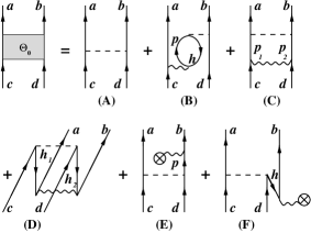
Figure 1: Second-order diagrams included in the perturbative expansion of $\hat{\Theta}$. The dashed lines indicate the bare operator $\Theta$, the wavy lines the two-body potential $V_{{\rm low}\mbox{-}k}$ (see text for details).

We point out that diagrams (A)-(D) belongs also to the perturbative expansion of $\Theta_{\rm eff}$ in Refs. Wu et al. (1985); Holt and Engel (2013), where diagrams (E) and (F) were neglected. The contribution of $(V_{{\rm low}\mbox{-}k}-U)$-insertion diagrams, such as (E) and (F), is equal to zero only under the hypothesis that the HO potential would correspond to a Hartree-Fock basis for the $V_{{\rm low}\mbox{-}k}$ potential. In a previous study, we have shown that the role of this class of diagrams is non-negligible to derive $H_{\rm eff}$, in particular to benchmark RSM with ab initio calculations Coraggio et al. (2012).

So far we have presented the derivation of an effective operator just for a nuclear system with two valence nucleons, but in the following section we are going to focus on $0\nu\beta\beta$ decay of nuclei that, within the shell-model, will be described in terms of a number of valence nucleons that is much larger than 2. For example double-$\beta$ decay of ¹³⁶Xe into ¹³⁶Te involves 36 valence nucleons outside the doubly-magic ¹⁰⁰Sn, and in such a case the expression of $\Theta_{\rm eff}$ should contain contribution up to a 36-body term.

At present this is unfeasible, so we include just the leading terms of these many-body contributions in the perturbative expansion of $\hat{\Theta}$, namely the second-order three-body diagrams (a) and (b), that are reported in Fig. 2. For the sake of simplicity, for each topology only one of the diagrams which correspond to the permutation of the external lines is drawn.

Figure 2: Second-order three-body diagrams which are included in the perturbative expansion of $\hat{\Theta}$. As in Fig. 1, the dashed line indicates the bare operator $\Theta$, the wavy line the two-body potential $V_{{\rm low}\mbox{-}k}$.

The two topologies of second-order connected three-valence-nucleon diagrams (a) and (b) correct the Pauli-principle violation introduced by diagram (a’) and (b’) when one of the intermediate particle states is equal to $m$ Ellis and Osnes (1977). This is the so-called “blocking effect”, which urges to take into account the Pauli exclusion principle in systems with more than two valence nucleons Towner (1987).

It should be pointed out that also the authors of Ref. Holt and Engel (2013) have attempted to account for this effect in an approximate way, by weighting the intermediate model-space-particle lines that appear in the $\hat{\Theta}$-box diagrams with a factor that suppress their matrix elements in terms of the unperturbed occupation density of the line orbital.

Since the NATHAN SM code, that we employ to calculate $M^{0\nu}$ Caurier and Martinez-Pinedo (2002), cannot manage three-body decay operators, we have derived a density-dependent two-body contribution at one-loop order from the three-body diagrams in Fig. 2, summing over the partially-filled model-space orbitals. The details of this procedure can be found in Ref. Itaco et al. (2019), as well as in Ref. Ma et al. (2019), where the same procedure has been preformed to derive density-dependent two-body $H_{\rm eff}$s  to study many-valence nucleon systems.

II.3 The $0\nu\beta\beta$-decay operator

We now focus our attention on the vertices of the bare $0\nu\beta\beta$ operator $\Theta$.

We recall that the formal expression of $M_{\alpha}^{0\nu}$ - $\alpha$ denoting the Fermi ($F$), Gamow-Teller (GT), or tensor ($T$) decay channels - is written in terms of the one-body transition-density matrix elements between the daughter and parent nuclei (grand-daughter and daughter nuclei) $\langle k|a^{\dagger}_{p^{\prime}}a_{n^{\prime}}|i\rangle$ ($\langle f|a^{\dagger}_{p}a_{n}|k\rangle$), $p,n$ subscripts denoting proton and neutron states, and indices $i,k,f$ the parent, daughter, and grand-daughter nuclei, respectively:

$$M_{\alpha}^{0\nu} = \sum_{k}\sum_{j_{p}j_{p^{\prime}}j_{n}j_{n^{\prime}}}\langle f|a^{\dagger}_{p}a_{n}|k\rangle\langle k|a^{\dagger}_{p^{\prime}}a_{n^{\prime}}|i\rangle$$

$$\times\left<j_{p}j_{p^{\prime}}\mid\tau^{-}_{1}\tau^{-}_{2}\Theta_{\alpha}^{k}\mid j_{n}j_{n^{\prime}}\right>~{}.$$ (15)

The operators $\Theta_{\alpha}$ are expressed in terms of the neutrino potentials $H_{\alpha}$ and form functions $h_{\alpha}(q)$:

$$\Theta^{k}_{\rm GT} = \vec{\sigma}_{1}\cdot\vec{\sigma}_{2}H_{\rm GT}^{k}(r)$$ (16)

$$\Theta^{k}_{\rm F} = H_{\rm F}^{k}(r)$$ (17)

$$\Theta^{k}_{\rm T} = \left[3\left(\vec{\sigma}_{1}\cdot\hat{r}\right)\left(\vec{\sigma}_{1}\cdot\hat{r}\right)-\vec{\sigma}_{1}\cdot\vec{\sigma}_{2}\right]H_{\rm T}^{k}(r)~{},$$ (18)

$$H_{\alpha}^{k}(r)=\frac{2R}{\pi}\int_{0}^{\infty}\frac{j_{n_{\alpha}}(qr)h_{\alpha}(q^{2})qdq}{q+E_{k}-(E_{i}+E_{f})/2}~{}.$$ (19)

The value of the parameter $R$ is $R=1.2A^{1/3}$ fm, the $j_{n_{\alpha}}(qr)$ are the spherical Bessel functions, $n_{\alpha}=0$ for Fermi and Gamow-Teller components, $n_{\alpha}=2$ for the tensor one. For the sake of clarity, the explicit expression of neutrino form functions $h_{\alpha}(q)$ for light-neutrino exchange we employ in present calculations are reported below:

$$h_{F}({q}^{2}) = g^{2}_{V}({q}^{2})$$

$$h_{GT}({q}^{2}) = \frac{g^{2}_{A}({q}^{2})}{g^{2}_{A}}\left[1-\frac{2}{3}\frac{{q}^{2}}{{q}^{2}+m^{2}_{\pi}}+\frac{1}{3}(\frac{{q}^{2}}{{q}^{2}+m^{2}_{\pi}})^{2}\right]$$

$$+\frac{2}{3}\frac{g^{2}_{M}({q}^{2})}{g^{2}_{A}}\frac{{q}^{2}}{4m^{2}_{p}},$$

$$h_{T}({q}^{2}) = \frac{g^{2}_{A}({q}^{2})}{g^{2}_{A}}\left[\frac{2}{3}\frac{{q}^{2}}{{q}^{2}+m^{2}_{\pi}}-\frac{1}{3}(\frac{{q}^{2}}{{q}^{2}+m^{2}_{\pi}})^{2}\right]$$ (20)

$$+\frac{1}{3}\frac{g^{2}_{M}({q}^{2})}{g^{2}_{A}}\frac{{q}^{2}}{4m^{2}_{p}}$$

The dipole approximation has been adopted for the vector, axial-vector and weak-magnetism $g_{V}({q}^{2}),g_{A}({q}^{2}),g_{M}({q}^{2})$ form factors :

$$g_{V}({q}^{2}) = \frac{g_{V}}{(1+{q}^{2}/{\Lambda^{2}_{V}})^{2}},$$

$$g_{M}({q}^{2}) = (\mu_{p}-\mu_{n})g_{V}({q}^{2}),$$

$$g_{A}({q}^{2}) = \frac{g_{A}}{(1+{q}^{2}/{\Lambda^{2}_{A}})^{2}},$$ (21)

where $g_{V}=1$, $g_{A}\equiv g_{A}^{free}=1.2723$, $(\mu_{p}-\mu_{n})=3.70$, and the cutoff parameters $\Lambda_{V}=850$ MeV and $\Lambda_{A}=1086$ MeV.

The expression in Eq. (15) can be easier managed computationally within the QRPA, while all other models - including most of SM calculations - resort to the so-called closure approximation. This approximation is based on the fact that the relative momenta $q$ of the neutrinos involved in the decay, appearing in the denominator of the neutrino potential of Eq. (19), are of the order of 100-200 MeV, while the excitation energies of the nuclei involved in the $0\nu\beta\beta$decay are only of the order of 10 MeV Sen’kov and Horoi (2013).

The above considerations lead to replace the energies of the intermediate states $E_{k}$ in Eq. (19) by an average value $E_{k}-(E_{i}+E_{f})/2\rightarrow\langle E\rangle$, and simplify both the relationships (15, 19). $M_{\alpha}^{0\nu}$ can be re-written in terms of the two-body transition-density matrix elements $\langle f|a^{\dagger}_{p}a_{n}a^{\dagger}_{p^{\prime}}a_{n^{\prime}}|i\rangle$:

$$M_{\alpha}^{0\nu} = \sum_{j_{n}j_{n^{\prime}}j_{p}j_{p^{\prime}}}\langle f|a^{\dagger}_{p}a_{n}a^{\dagger}_{p^{\prime}}a_{n^{\prime}}|i\rangle$$

$$\times\left<j_{p}j_{p^{\prime}}\mid\tau^{-}_{1}\tau^{-}_{2}\Theta_{\alpha}\mid j_{n}j_{n^{\prime}}\right>~{},$$ (22)

and the neutrino potential are expressed as:

$$H_{\alpha}(r)=\frac{2R}{\pi}\int_{0}^{\infty}\frac{j_{n_{\alpha}}(qr)h_{\alpha}(q^{2})qdq}{q+\left<E\right>}~{}.$$ (23)

In present calculations, we adopt the closure approximation to define the operators $\Theta$ in Eqs. (16-18), and the average energies $\left<E\right>$ have been evaluated as in Refs. Haxton and Stephenson Jr. (1984); Tomoda (1991). It should be noted that the closure approximation simplifies the derivation of $\Theta_{\rm eff}$, since the diagrams appearing in the perturbative expansion of the vertex function $\hat{\Theta}$ will not be dependent on the energy of the daughter-nucleus intermediate states $E_{k}$.

In this regard, the authors of Ref. Sen’kov and Horoi (2013) have performed SM calculations of $M^{0\nu}$ for ⁴⁸Ca $0\nu\beta\beta$ decay both within and beyond closure approximation, and have shown that the results beyond closure-approximation are $10\%$ larger.

Now, it is worth to recollect the main motivations to renormalize the $0\nu\beta\beta$-decay operator, as we have already mentioned in the Introduction:

1. The truncation of the $A$-body problem in the full Hilbert space to the problem of few valence nucleons interacting in the reduced model space.

2. The contribution of the short-range correlations (SRC), accounting the fact that the action of a two-body decay operator on an unperturbed (uncorrelated) wave function, that is used in the perturbative expansion of $\Theta_{\rm eff}$ is not equal to the action of the same operator on the real (correlated) nuclear wave function.

3. The contribution of the two-body meson-exchange corrections to the electroweak currents, originated from sub-nucleonic degrees of freedom.

Up to this point, we have extensively covered point (a), and we need to discuss about issues (b) and (c).

As regards the inclusion of the SRC, in Ref. Coraggio et al. (2019b) we have introduced an original approach that is consistent with the $V_{{\rm low}\mbox{-}k}$ procedure. More precisely, the $0\nu\beta\beta$  operator $\Theta$ is calculated within the momentum space and then renormalized by way of $\Omega$ in order to consider effectively the high-momentum (short range) components of the $NN$ potential, in a framework where their direct contribution is dumped by the introduction of a cutoff $\Lambda$.

Consequently, the $\Theta$ vertices appearing in the perturbative expansion of the $\hat{\Theta}$ box are subsituted with the renormalized $\Theta_{{\rm low}\mbox{-}k}$ operator that is defined as $\Theta_{{\rm low}\mbox{-}k}\equiv P\Omega\Theta\Omega^{-1}P$ for relative momenta $k<\Lambda$, and is equal to zero for $k>\Lambda$.

We have found that the effect in magnitude of this renormalization procedure is similar to the SRC modeled by the so-called Unitary Correlation Operator Method (UCOM) Menéndez et al. (2009b), meaning a lighter softening of $M^{0\nu}$ with respect to the one provided by Jastrow type SRC.

The last issue to be considered is the the role of meson-exchange corrections to the electroweak currents, that has been also investigated in Refs. Menéndez et al. (2011); Wang et al. (2018). The framework of these studies is the Chiral Effective Field Theory (ChEFT) that allows a consistent derivation of nuclear two- and three-body forces, as well as electroweak chiral two-body currents which are characterized by the same low-energy constants (LECs) appearing in the structure of the nuclear Hamiltonian.

In our calculations we start from the CD-Bonn potential, and then renormalize it by way of the $V_{{\rm low}\mbox{-}k}$  procedure, preventing us to approach issue (c) in a way that is consistent with the derivation of our starting two-body force (as we do for the treatment of SRC). However, we are confident that, since we employ a large cutoff ($\Lambda=2.6$ fm^-1) for the derivation of $V_{{\rm low}\mbox{-}k}$, our results are less affected by residual three-body force contributions and, consequently, by electroweak two-body current corrections.

III Results

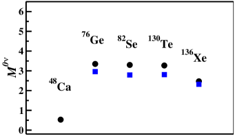
Figure 3: Calculated values of $M^{0\nu}$ for ⁴⁸Ca, ⁷⁶Ge, ⁸²Se, ¹³⁰Te, and ¹³⁶Xe decays (black dots), obtained from the bare $0\nu\beta\beta$ decay operator. The results are compared with those reported in Ref. Menéndez et al. (2009b) (blue squares), and obtained without including SRC.

We recall that our calculations of $M^{0\nu}$ account for the light-neutrino exchange mechanism, and that the effective Hamiltonians we have employed are those reported in Refs.Coraggio et al. (2017); Coraggio et al. (2019a), where it can be found a detailed description of the low-energy spectroscopic properties of ⁴⁸Ca, ⁷⁶Ge, ⁸²Se, ¹³⁰Te, and ¹³⁶Xe, obtained with their diagonalization. In present work we neglect the contribution of the tensor component of Eq. (18), since it plays a minor role, its matrix elements being about two order of magnitude smaller than those corresponding to the Gamow-Teller and Fermi decay operators. Actually, it should be pointed out that the ⁴⁸Ca decay is an exception, since the ratio of the tensor component to the GT contribution may reach the value of $10\%$ Menéndez et al. (2009b).

In our calculations, the total nuclear matrix element $M^{0\nu}$ is expressed as

$$M^{0\nu}=M^{0\nu}_{\rm GT}-\left(\frac{g_{V}}{g_{A}}\right)^{2}M^{0\nu}_{\rm F}~{},$$ (24)

and depends on the axial and vector coupling constants $g_{A},g_{V}$, the free values being $g_{A}^{free}=1.2723,~{}g_{V}^{free}=1$ Tanabashi et al. (2018).

The nuclear matrix elements $M^{0\nu}_{\rm GT,F}$ are calculated accordingly Eqs. (16,17,22,23), namely within the closure approximation.

The first results it is worth presenting are the calculated $M^{0\nu}$values for the nuclei under investigation, obtained with the bare decay-operator $\Theta$, without any contribution from the renormalization procedure (see Fig. 3).

We compare the results of our calculations (black dots) with those obtained in similar SM calculations employing the same model spaces and the same $0\nu\beta\beta$ decay operator, that is the one without any kind of renormalization. More precisely, we refer to the calculations by Madrid-Strasbourg group (blue squares) (see the first column in Table 8 in Ref. Menéndez et al. (2009b)). It is worth pointing out that the results represented by the blue squares include also the tensor component of $M^{0\nu}$, but the authors have found that $M^{0\nu}_{\rm T}$ contribution for ⁷⁶Ge, ⁸²Se, ¹³⁰Te, and ¹³⁶Xe decays is less than $1\%$ of the dominant GT one Menéndez et al. (2009b).

Since the two-body matrix elements of $\Theta$ are the same, this comparison can be considered a sort of benchmark of the nuclear SM wave functions, that have been obtained starting from different $H_{\rm eff}$s. As a matter of fact, the TBME of $H_{\rm eff}$s employed in Ref. Menéndez et al. (2009b) have been derived as a fine tuning of TBME obtained from realistic SM $H_{\rm eff}$s Hjorth-Jensen et al. (1995). The modifications have been made to fit to some specific spectroscopic data of nuclei in $pf$, $f_{5/2}pg_{9/2}$, and $g_{7/2}dsh_{11/2}$ regions, as well as single-particle properties in the same regions to determine the SP energies (details can be found in the above mentioned papers and references therein).

Figure 4: $M^{0\nu}$ for the ${}^{76}\mbox{Ge}\rightarrow^{76}$Se decay as a function of $N_{\rm max}$. The red diamonds correspond to a truncation of $\chi_{n}$ expansion up to $\chi_{0}$, blue squares up to $\chi_{1}$, and black dots up to $\chi_{2}$.

As described in Section II, our $H_{\rm eff}$s have been derived from a realistic $V_{NN}$ and their matrix elements have been not modified to improve the agreement with experiment. As can be seen from inspection of Fig. 3, there is a general agreement among the different calculations, that is linked to a common quality of the different $H_{\rm eff}$s to reproduce satisfactorily a large amount of spectra in these mass regions.

Figure 5: $M^{0\nu}$ for the ${}^{48}\mbox{Ca}\rightarrow^{48}$Ti decay as a function of the perturbative order. The green triangles correspond to $M^{0\nu}_{\rm F}$, the blue squares to $M^{0\nu}_{\rm GT}$, and the black dots to the full $M^{0\nu}$.

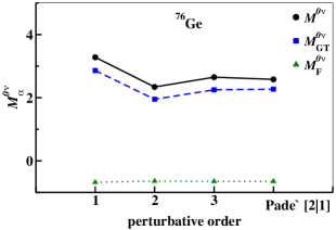
Figure 6: Same as in Fig. 5, but for the ${}^{76}\mbox{Ge}\rightarrow^{76}$Se decay.

We shift now the focus on the results of the calculations obtained by employing the effective decay-operator $\Theta_{\rm eff}$, which accounts for the truncation of the Hilbert space, the SRC, and the Pauli-blocking effect as well.

First, we report about the convergence properties with respect to the number of intermediate states included in the perturbative expansion of $\Theta_{\rm eff}$, and the truncation of the order of $\chi_{n}$ operators.

In Fig. 4 the calculated values of $M^{0\nu}$ for the ${\rm{}^{76}Ge}\rightarrow{\rm{}^{76}Se}$ decay are reported as a function of the maximum allowed excitation energy of the intermediate states expressed in terms of the oscillator quanta $N_{\rm max}$, and for contributions up to the $\chi_{2}$ operator. The plot shows that the results are substantially convergent from $N_{\rm max}=12$ on and the contributions from $\chi_{1}$ are crucial while those from $\chi_{2}$ are almost negligible.

It is worth pointing out that $\chi_{3}$ depends on the first, second, and third derivatives of $\hat{\Theta}_{0}$ and $\hat{\Theta}_{00}$, as well as on the first and second derivatives of the $\hat{Q}$ box (see Eq. (II.2)), so we estimate $\chi_{3}$ contribution being at least one order of magnitude smaller than the $\chi_{2}$ one.

On the basis of the above analysis, the results we report in this Section are all obtained including in the perturbative expansion up to third-order diagrams, whose number of intermediate states corresponds to oscillator quanta up to $N_{\rm max}=14$, and up to $\chi_{2}$ contributions.

Now, we consider the order-by-order convergence behavior by reporting in Figs. 5-9 the calculated values of $M^{0\nu}$, $M^{0\nu}_{\rm GT}$, and $M^{0\nu}_{\rm F}$ for ⁴⁸Ca, ⁷⁶Ge, ⁸²Se, ¹³⁰Te, and ¹³⁶Xe$0\nu\beta\beta$ decay, respectively, from first- up to third-order in perturbation theory. We compare the order-by-order results also with their Padé approximant $[2|1]$, as an indicator of the quality of the perturbative behavior Baker and Gammel (1970). It should be pointed out that the same scale has been employed in all the figures.

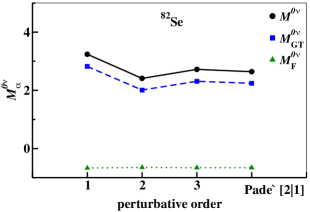
Figure 7: Same as in Fig. 5, but for the ${}^{82}\mbox{Se}\rightarrow^{82}$Kr decay.

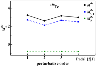
Figure 8: Same as in Fig. 5, but for the ${}^{130}\mbox{Te}\rightarrow^{130}$Xe decay.

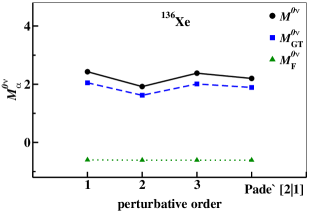
Figure 9: Same as in Fig. 5, but for the ${}^{136}\mbox{Xe}\rightarrow^{136}$Ba decay.

First of all, we observe that the perturbative behavior is dominated by the Gamow-Teller component, since the renormalization procedure does not affect significantly the Fermi matrix element $M^{0\nu}_{\rm F}$. We recall that the perturbative behavior of the single $\beta$-decay operator provides a difference between the $M^{2\nu}$values calculated at second and third order in perturbation theory which does not exceed $10\%$ Coraggio et al. (2018). Here, we observe a less satisfactory perturbative behavior for our calculation of $M^{0\nu}$, the difference between second- and third-order results being about $15\%$ and $30\%$ for ⁷⁶Ge, ⁸²Se, and ¹³⁰Te,¹³⁶Xe $0\nu\beta\beta$ decays, respectively.

The calculation of $M^{0\nu}$ for ⁴⁸Ca $0\nu\beta\beta$ decay exhibits the worst perturbative behavior. In such a case, we observe a difference between the second- and third-order results which is almost $50\%$, and this puzzling outcome deserves a more specific discussion when the study of the GT matrix elements in terms of the contributions from the decaying pair of neutrons coupled to a given angular momentum and parity $J^{\pi}$ will be reported in Figs. 10-14.

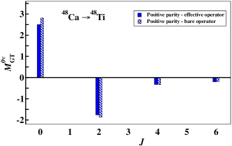
Figure 10: Contributions from pairs of decaying neutrons with given $J^{\pi}$ to $M^{0\nu}_{\rm GT}$ for ⁴⁸Ca $0\nu\beta\beta$ decay. The bars filled in blue corresponds to the results obtained with $\Theta_{\rm eff}$, those in dashed blue to the ones calculated with bare operator

The issue of the perturbative behavior needs to be addressed, and in this connection the calculation of $M^{0\nu}$ beyond the closure approximation may lead to an improvement. In fact, the energy denominator of neutrino potentials in Eq. (19) depends on the energies of real intermediate states, and the inclusion of this dependence in the calculation of virtual intermediate states in the perturbative expansion of $\Theta_{\rm eff}$ may strongly influence the order-by-order perturbative behavior.

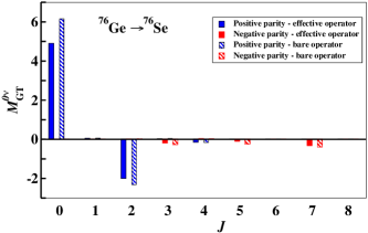
Figure 11: Same as in Fig. 10, but for ⁷⁶Ge $0\nu\beta\beta$ decay. The red bars corresponds to negative-parity states.

Figure 12: Same as in Fig. 11, but for ⁸²Se $0\nu\beta\beta$ decay.

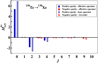
Figure 13: Same as in Fig. 11, but for ¹³⁰Te $0\nu\beta\beta$ decay.

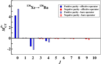
Figure 14: Same as in Fig. 11, but for ¹³⁶Xe $0\nu\beta\beta$ decay.

As mentioned before, we perform a decomposition of $M^{0\nu}_{\rm GT}$ in terms of the contributions from the decaying pair of neutrons coupled to a given angular momentum and parity $J^{\pi}$, and the results are reported in Figs. 10-14. We compare the contributions obtained from calculations performed by employing both the effective $0\nu\beta\beta$-decay operator $\Theta_{\rm eff}$ and the bare one, without any renormalization contribution.

As a general remark, we see that each $J^{\pi}$ contribution to $M^{0\nu}_{\rm GT}$ calculated employing $\Theta_{\rm eff}$ is smaller than the one obtained with the bare $0\nu\beta\beta$-decay operator. This corresponds to a quenching of each Gamow-Teller component, in terms of the $J^{\pi}$ decomposition. Actually, the main contributions, for both the effective and the bare operators, are provided by $J^{\pi}=0^{+},2^{+}$ components and they are always opposite in sign. A non-negligible role is also played by the $J^{\pi}=4^{+}$ component for ¹³⁰Te,¹³⁶Xe decays.

Table 1: Calculated values of $M^{0\nu}$ for all decays under investigation. The first column corresponds to the results ontained employing the bare $0\nu\beta\beta$-decay operator, the second one to the calculations performed with $\Theta_{\rm eff}$. The third column corresponds to calculating $\Theta_{\rm eff}$ without corrections due to the Pauli-blocking effect.

Decay	bare operator	$\Theta_{\rm eff}$	$\Theta_{\rm eff}$ - no Pauli
48Ca $\rightarrow$ 48Ti	0.53	0.30	0.30
76Ge $\rightarrow$ 76Se	3.35	2.66	3.01
82Se $\rightarrow$ 82Kr	3.30	2.72	2.94
130Te $\rightarrow$ 130Xe	3.27	3.16	2.98
136Xe $\rightarrow$ 136Ba	2.47	2.39	2.24

The quenching of GT $J^{\pi}$ components reflects also on the comparison between the full $M^{0\nu}$ calculated with the bare and effective $0\nu\beta\beta$-decay operator, as can be seen in the values reported in Table 1. In the same table we also report the values of $M^{0\nu}$ obtained without the inclusion of the three-body contributions of Fig. 2, which are intended to account for the Pauli exclusion principle in many-valence-nucleons systems and correct the “blocking effect”.

For the sake of the completeness, we point out that our results of the $J^{\pi}$ decomposition are similar to those obtained in other SM calculations, as for example in Ref. Sen’kov and Horoi (2013, 2016); Sen’kov et al. (2014); Jiao et al. (2018) for ⁴⁸Ca, ⁷⁶Ge, ⁸²Se, ¹³⁰Te, and ¹³⁶Xe decays, respectively.

A long standing issue about the calculation of $M^{0\nu}$ is wether there is a connection between the derivation of the effective one-body GT operator Coraggio et al. (2019a) and the renormalization of the two-body GT component of the $0\nu\beta\beta$ operator, or not. Namely, some authors argue that the quenching factor that is needed to match theory and experiment of GT-decay properties (single-$\beta$ decay strengths, $M^{2\nu}$s, etc.) should be also employed to calculate $M^{0\nu}$, with a large impact on the detectability of $0\nu\beta\beta$ process (see for instance Refs. Suhonen (2017b, a)).

It is worth to observe that, from our results of the calculation of $M^{2\nu}$s using both bare and effective single-$\beta$ decay operators (see Tables II, IV, VI, and VIII in Ref. Coraggio et al. (2019a)), we may induce quenching factors of the axial coupling constant $g_{A}$ that are $q=0.83,0.58,0.56,0.68,0.61$ for ⁴⁸Ca, ⁷⁶Ge, ⁸²Se, ¹³⁰Te, and ¹³⁶Xe decays, respectively.

If these quenching factors were employed to calculate $M^{0\nu}$, starting from the bare $0\nu\beta\beta$-decay operator, we would obtain $M^{0\nu}$=0.40,1.41,1.32,1.78,1.15 for the above corresponding decays.

The comparison of these numbers with those in Table 1 evidences the different mechanisms which underlies the renormalization of the one-body single-$\beta$ and the two-body $0\nu\beta\beta$ decay operators, the first one leading to quenching factors which might strongly suppress the calculated $M^{0\nu}$s.

Now, as mentioned above, it is worth to come back to the discussion about the perturbative behavior of the effective $0\nu\beta\beta$-decay operator for ${}^{48}\mbox{Ca}\rightarrow^{48}$Ti. From the inspection of Fig. 10, we observe a large cancelation between the $J^{\pi}=0^{+}$ and $J^{\pi}=2^{+}$ components, leading to a $M^{0\nu}$value that is the smallest among the nuclear matrix elements we have calculated. This is a characteristic that our results share with other SM calculations such as those, for example, in Refs. Menéndez et al. (2009b); Sen’kov and Horoi (2013).

In Fig. 15 we compare the results of the $J^{\pi}$ decomposition we obtain employing, for ⁴⁸Ca decay, the effective $0\nu\beta\beta$ operator calculated both at second and third order in perturbation theory.

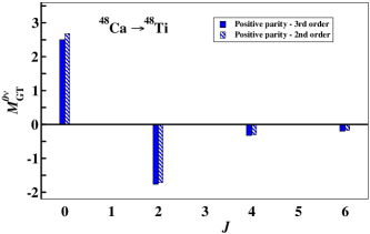
Figure 15: Contributions from pairs of decaying neutrons with given $J^{\pi}$ to $M^{0\nu}_{\rm GT}$ for ⁴⁸Ca $0\nu\beta\beta$ decay. The bars filled in blue corresponds to the results obtained with $\Theta_{\rm eff}$ calculated a third order in perturbation theory (as in Fig. 10), those in dashed blue are calculated at second order.

As can be seen, the order-by-order convergence of each component of $M^{0\nu}_{\rm GT}$ is quite good, and the difference between second and third order does not exceed $7\%$ for the two main contributions $J^{\pi}=2^{+},4^{+}$. However, the cancelation between these two $J^{\pi}$ component enhances the oscillation between the total result at second and third order in perturbation theory, the difference between them increasing to $50\%$.

Finally, we would like to comment the comparison between the results reported in the last two columns in Table 1, that evidences the role played by the “blocking effect”. As can be seen, the difference between the last two columns - results with and without accounting for the Pauli-principle violations - is at most about $12\%$ for ⁷⁶Ge decay, being less than $10\%$ in all other decays. In Ref. Coraggio et al. (2019a) we have found that the contribution of the “blocking effect” in the $2\nu\beta\beta$  decay has more or less the same magnitude, but it always enlarges $M^{2\nu}$. In the present calculations, we observe a decrease of $M^{0\nu}$ for ⁷⁶Ge and ⁸²Se $0\nu\beta\beta$ decays, and an increase for ¹³⁰Te and ¹³⁶Xe $0\nu\beta\beta$ decays. This feature is related to a different balance between the role of diagrams (a) and (b) (see Fig. 2) in the perturbative expansion of $\Theta_{\rm eff}$, these diagrams suppressing the Pauli-principle violating contribution of diagrams (a’) and (b’) (see Table 3 in Ref. Itaco et al. (2019)).

IV Summary and outlook

The work presented in this paper has been devoted to the calculation, within the realistic shell model, of the nuclear matrix element $M^{0\nu}$ relative to the $0\nu\beta\beta$decay. To this end, shell-model effective Hamiltonians and operators have been derived by way of many-body perturbation theory, starting from a realistic $NN$ potential renormalized through the $V_{{\rm low}\mbox{-}k}$ approach Bogner et al. (2002).

Our study has been focussed on the ⁴⁸Ca$\rightarrow^{48}$Ti, ⁷⁶Ge$\rightarrow^{76}$Se, ⁸²Se$\rightarrow^{82}$Kr, ¹³⁰Te$\rightarrow^{130}$Xe, and ¹³⁶Xe$\rightarrow^{136}$Ba decays, as a continuation of a previous work where we have addressed the reliability of the realistic shell model to calculate, by way of theoretical SM effective operators, the nuclear matrix elements $M^{2\nu}$s for the $2\nu\beta\beta$  decay involving the same nuclei of present investigation Coraggio et al. (2019a). The results that have been obtained and shown in that paper support the ability of realistic shell model to provide a quantitative description of data relative to both spectroscopy (low-lying excitation spectra, electromagnetic transition strengths) and $\beta$ decay (nuclear matrix elements of $2\nu\beta\beta$ decay, GT strengths from charge-exchange reactions) without resorting to empirical adjustments of $H_{\rm eff}$, effective charges or gyromagnetic factors, or to the quenching of the axial coupling constant.

We may summarise the main results of present study into two statements:

• the order-by-order perturbative behavior of the calculated effective two-body $0\nu\beta\beta$-decay operator is not as satisfactory as the one relative to the perturbative expansion of the effective one-body single-$\beta$ decay operator Coraggio et al. (2018). The issue of the perturbative behavior of effective SM Hamiltonians and operators is relevant to assess the evaluation of theoretical uncertainties.

• Even if our results may be still significantly improved, we can assert that the effect of the renormalization of the $0\nu\beta\beta$-decay operator, with respect to the truncation of the full Hilbert space to the shell-model one, is far less important than that regarding the well-known problem of the $g_{A}$ quenching Suhonen (2017a, b). Namely, the $M^{0\nu}$s calculated using the effective $0\nu\beta\beta$-decay operator are quite larger than those calculated employing a quenching factor deduced by our results for the $2\nu\beta\beta$-decay (see Section III).

Our present and near future efforts, on one side, are and will be devoted to improve the perturbative behavior of the order-by-order expansion of the effective $0\nu\beta\beta$  operator. As we have mentioned in the previous Section, we are confident that overcoming the limits of the closure approximation this goal may be achieved, even if this is a very demanding task in terms of computational resources.

On another side, we intend to deal with the renormalization of the $0\nu\beta\beta$  operator due to the subnucleonic degrees of freedom. This issue has to be consistently tackled starting from two- and three-body nuclear potentials derived within the framework of chiral perturbation theory Fukui et al. (2018); Ma et al. (2019), and taking also into account the contributions of chiral two-body electroweak currents. Some authors have found that $\beta$- and neutrinoless double-beta decays may be affected by these contributions Gysbers et al. (2019); Wang et al. (2018), even if it should be pointed out that a recent study evidences that, for standard GT transitions ($\beta$ decay, $2\nu\beta\beta$ decay), the many-body meson currents should play no significant role due to the “chiral filter” mechanism Rho (2019).

Actually, this mechanism may be no longer valid for $0\nu\beta\beta$ decay, the transferred momentum being $\sim 100$ MeV, and therefore we consider intriguing to carry out further investigations to grasp the role of exchange-current contributions.

At present, the derivation of effective SM Hamiltonians and operators for medium-mass nuclei - including also contributions of three-body nuclear potentials and many-body electroweak currents - is computationally challenging if one wants to achieve the same accuracy attained in present calculations, namely carrying out the perturbative expansion consistently up to the third order in perturbation theory.

References

- Avignone et al. (2008) F. T. Avignone, S. R. Elliott, and J. Engel, Rev. Mod. Phys. 80, 481 (2008).
- Dell’Oro et al. (2016) S. Dell’Oro, S. Marcocci, M. Viel, and F. Vissani, Adv. High Energy Phys. 2016, 2162659 (2016).
- Henning (2016) R. Henning, Reviews in Physics 1, 29 (2016), ISSN 2405-4283.
- Agostini et al. (2019) M. Agostini, A. M. Bakalyarov, M. Balata, I. Barabanov, L. Baudis, C. Bauer, E. Bellotti, S. Belogurov, A. Bettini, L. Bezrukov, et al. (GERDA Collaboration), Science 365, 1445 (2019).
- Alfonso et al. (2015) K. Alfonso, D. R. Artusa, F. T. Avignone, O. Azzolini, M. Balata, T. I. Banks, G. Bari, J. W. Beeman, F. Bellini, A. Bersani, et al. (CUORE Collaboration), Phys. Rev. Lett. 115, 102502 (2015).
- Gando et al. (2016) A. Gando, Y. Gando, T. Hachiya, A. Hayashi, S. Hayashida, H. Ikeda, K. Inoue, K. Ishidoshiro, Y. Karino, M. Koga, et al. (KamLAND-Zen Collaboration), Phys. Rev. Lett. 117, 082503 (2016).
- Buchmüller et al. (2005) W. Buchmüller, R. Peccei, and T. Yanagida, Annual Review of Nuclear and Particle Science 55, 311 (2005).
- Kotila and Iachello (2012) J. Kotila and F. Iachello, Phys. Rev. C 85, 034316 (2012).
- Kotila and Iachello (2013) J. Kotila and F. Iachello, Phys. Rev. C 87, 024313 (2013).
- Tanabashi et al. (2018) M. Tanabashi, K. Hagiwara, K. Hikasa, K. Nakamura, Y. Sumino, F. Takahashi, J. Tanaka, K. Agashe, G. Aielli, C. Amsler, et al. (Particle Data Group), Phys. Rev. D 98, 030001 (2018).
- Pastore et al. (2018) S. Pastore, J. Carlson, V. Cirigliano, W. Dekens, E. Mereghetti, and R. B. Wiringa, Phys. Rev. C 97, 014606 (2018).
- Barea and Iachello (2009) J. Barea and F. Iachello, Phys. Rev. C 79, 044301 (2009).
- Barea et al. (2012) J. Barea, J. Kotila, and F. Iachello, Phys. Rev. Lett. 109, 042501 (2012).
- Barea et al. (2013) J. Barea, J. Kotila, and F. Iachello, Phys. Rev. C 87, 014315 (2013).
- Šimkovic et al. (2009) F. Šimkovic, A. Faessler, H. Müther, V. Rodin, and M. Stauf, Phys. Rev. C 79, 055501 (2009).
- Fang et al. (2011) D.-L. Fang, A. Faessler, V. Rodin, and F. Šimkovic, Phys. Rev. C 83, 034320 (2011).
- Faessler et al. (2012) A. Faessler, V. Rodin, and F. Simkovic, J. Phys. G 39, 124006 (2012).
- Rodríguez and Martínez-Pinedo (2010) T. R. Rodríguez and G. Martínez-Pinedo, Phys. Rev. Lett. 105, 252503 (2010).
- Song et al. (2014) L. S. Song, J. M. Yao, P. Ring, and J. Meng, Phys. Rev. C 90, 054309 (2014).
- Yao et al. (2015) J. M. Yao, L. S. Song, K. Hagino, P. Ring, and J. Meng, Phys. Rev. C 91, 024316 (2015).
- Song et al. (2017) L. S. Song, J. M. Yao, P. Ring, and J. Meng, Phys. Rev. C 95, 024305 (2017).
- Jiao et al. (2017) C. F. Jiao, J. Engel, and J. D. Holt, Phys. Rev. C 96, 054310 (2017).
- Yao et al. (2018) J. M. Yao, J. Engel, L. J. Wang, C. F. Jiao, and H. Hergert, Phys. Rev. C 98, 054311 (2018).
- Jiao et al. (2018) C. F. Jiao, M. Horoi, and A. Neacsu, Phys. Rev. C 98, 064324 (2018).
- Jiao and Johnson (2019) C. Jiao and C. W. Johnson, Phys. Rev. C 100, 031303 (2019).
- Menéndez et al. (2009a) J. Menéndez, A. Poves, E. Caurier, and F. Nowacki, Phys. Rev. C 80, 048501 (2009a).
- Menéndez et al. (2009b) J. Menéndez, A. Poves, E. Caurier, and F. Nowacki, Nucl. Phys. A 818, 139 (2009b).
- Horoi and Brown (2013) M. Horoi and B. A. Brown, Phys. Rev. Lett. 110, 222502 (2013).
- Neacsu and Horoi (2015) A. Neacsu and M. Horoi, Phys. Rev. C 91, 024309 (2015).
- Brown et al. (2015) B. A. Brown, D. L. Fang, and M. Horoi, Phys. Rev. C 92, 041301 (2015).
- Engel and Menéndez (2017) J. Engel and J. Menéndez, Rep. Prog. Phys. 90, 046301 (2017).
- Towner (1987) I. S. Towner, Phys. Rep. 155, 263 (1987).
- Suhonen (2017a) J. T. Suhonen, Frontiers in Physics 5, 55 (2017a).
- Park et al. (1993) T. S. Park, D. P. Min, and M. Rho, Phys. Rep. 233, 341 (1993).
- Pastore et al. (2009) S. Pastore, L. Girlanda, R. Schiavilla, M. Viviani, and R. B. Wiringa, Phys. Rev. C 80, 034004 (2009).
- Piarulli et al. (2013) M. Piarulli, L. Girlanda, L. E. Marcucci, S. Pastore, R. Schiavilla, and M. Viviani, Phys. Rev. C 87, 014006 (2013).
- Baroni et al. (2016) A. Baroni, L. Girlanda, S. Pastore, R. Schiavilla, and M. Viviani, Phys. Rev. C 93, 015501 (2016).
- Coraggio et al. (2009) L. Coraggio, A. Covello, A. Gargano, N. Itaco, and T. T. S. Kuo, Prog. Part. Nucl. Phys. 62, 135 (2009).
- Kuo et al. (1995) T. T. S. Kuo, F. Krmpotić, K. Suzuki, and R. Okamoto, Nucl. Phys. A 582, 205 (1995).
- Hjorth-Jensen et al. (1995) M. Hjorth-Jensen, T. T. S. Kuo, and E. Osnes, Phys. Rep. 261, 125 (1995).
- Suzuki and Okamoto (1995) K. Suzuki and R. Okamoto, Prog. Theor. Phys. 93, 905 (1995).
- Coraggio et al. (2012) L. Coraggio, A. Covello, A. Gargano, N. Itaco, and T. T. S. Kuo, Ann. Phys. (NY) 327, 2125 (2012).
- Machleidt (2001) R. Machleidt, Phys. Rev. C 63, 024001 (2001).
- Bogner et al. (2002) S. Bogner, T. T. S. Kuo, L. Coraggio, A. Covello, and N. Itaco, Phys. Rev. C 65, 051301(R) (2002).
- Bethe (1971) H. A. Bethe, Annu. Rev. Nucl. Sci. 21, 93 (1971).
- Kortelainen et al. (2007) M. Kortelainen, O. Civitarese, J. Suhonen, and J. Toivanen, Phys. Lett. B 647, 128 (2007).
- Coraggio et al. (2017) L. Coraggio, L. De Angelis, T. Fukui, A. Gargano, and N. Itaco, Phys. Rev. C 95, 064324 (2017).
- Coraggio et al. (2019a) L. Coraggio, L. De Angelis, T. Fukui, A. Gargano, N. Itaco, and F. Nowacki, Phys. Rev. C 100, 014316 (2019a).
- Wu et al. (1985) H. F. Wu, H. Q. Song, T. T. S. Kuo, W. K. Cheng, and D. Strottman, Phys. Lett. B 162, 227 (1985).
- Song et al. (1991) H. Q. Song, H. F. Wu, and T. T. S. Kuo, Phys. Lett. B 259, 229 (1991).
- Holt and Engel (2013) J. D. Holt and J. Engel, Phys. Rev. C 87, 064315 (2013).
- Lacombe et al. (1980) M. Lacombe, B. Loiseau, J. M. Richard, R. V. Mau, J. Côtè, P. Pirés, and R. D. Tourreil, Phys. Rev C 21, 861 (1980).
- Reid (1968) R. V. Reid, Ann. Phys. (N.Y.) 50, 411 (1968).
- Entem and Machleidt (2002) D. R. Entem and R. Machleidt, Phys. Rev. C 66, 014002 (2002).
- Horoi (2013) M. Horoi, J. Phys. Conf. Ser. 413, 012020 (2013).
- Coraggio et al. (2019b) L. Coraggio, N. Itaco, and R. Mancino, arXiv:1910.04146[nucl-th] (2019b), to be published in the Conference Proceedings of the 27th International Nuclear Physics Conference, 29 July - 2 August 2019, Glasgow (UK).
- Coraggio et al. (2015) L. Coraggio, A. Gargano, and N. Itaco, JPS Conf. Proc. 6, 020046 (2015).
- Kuo and Osnes (1990) T. T. S. Kuo and E. Osnes, Lecture Notes in Physics, vol. 364 (Springer-Verlag, Berlin, 1990).
- Kuo et al. (1971) T. T. S. Kuo, S. Y. Lee, and K. F. Ratcliff, Nucl. Phys. A 176, 65 (1971).
- Coraggio et al. (2010) L. Coraggio, A. Covello, A. Gargano, and N. Itaco, Phys. Rev. C 81, 064303 (2010).
- Coraggio et al. (2018) L. Coraggio, L. De Angelis, T. Fukui, A. Gargano, and N. Itaco, J. Phys. Conf. Ser. 1056, 012012 (2018).
- Krenciglowa and Kuo (1974) E. M. Krenciglowa and T. T. S. Kuo, Nucl. Phys. A 235, 171 (1974).
- Blomqvist and Molinari (1968) J. Blomqvist and A. Molinari, Nucl. Phys. A 106, 545 (1968).
- Ellis and Osnes (1977) P. J. Ellis and E. Osnes, Rev. Mod. Phys. 49, 777 (1977).
- Caurier and Martinez-Pinedo (2002) E. Caurier and G. Martinez-Pinedo, Nucl. Phys. A 704, 60c (2002).
- Itaco et al. (2019) N. Itaco, L. Coraggio, and R. Mancino, Eur. Phys. J. Web of Conferences 223, 01025 (2019).
- Ma et al. (2019) Y. Z. Ma, L. Coraggio, L. De Angelis, T. Fukui, A. Gargano, N. Itaco, and F. R. Xu, Phys. Rev. C 100, 034324 (2019).
- Sen’kov and Horoi (2013) R. A. Sen’kov and M. Horoi, Phys. Rev. C 88, 064312 (2013).
- Haxton and Stephenson Jr. (1984) W. C. Haxton and G. J. Stephenson Jr., Prog. Part. Nucl. Phys. 12, 409 (1984).
- Tomoda (1991) T. Tomoda, Rep. Prog. Phys. 54, 53 (1991).
- Menéndez et al. (2011) J. Menéndez, D. Gazit, and A. Schwenk, Phys. Rev. Lett. 107, 062501 (2011).
- Wang et al. (2018) L.-J. Wang, J. Engel, and J. M. Yao, Phys. Rev. C 98, 031301 (2018).
- Baker and Gammel (1970) G. A. Baker and J. L. Gammel, The Padé Approximant in Theoretical Physics, vol. 71 of Mathematics in Science and Engineering (Academic Press, New York, 1970).
- Sen’kov and Horoi (2016) R. A. Sen’kov and M. Horoi, Phys. Rev. C 93, 044334 (2016).
- Sen’kov et al. (2014) R. A. Sen’kov, M. Horoi, and B. A. Brown, Phys. Rev. C 89, 054304 (2014).
- Suhonen (2017b) J. Suhonen, Phys. Rev. C 96, 055501 (2017b).
- Fukui et al. (2018) T. Fukui, L. De Angelis, Y. Z. Ma, L. Coraggio, A. Gargano, N. Itaco, and F. R. Xu, Phys. Rev. C 98, 044305 (2018).
- Gysbers et al. (2019) P. Gysbers, G. Hagen, J. D. Holt, G. R. Jansen, T. D. Morris, P. Navrátil, T. Papenbrock, S. Quaglioni, A. Schwenk, S. R. Stroberg, et al., Nature Phys. 15, 428 (2019).
- Rho (2019) M. Rho, arXiv:1903.09976[nucl-th] (2019).