Ergodic Sum Rate Analysis of UAV-Based Relay Networks with Mixed RF-FSO Channels

Abstract

Unmanned aerial vehicle (UAV)-based communications is a promising new technology that can add a wide range of new capabilities to the current network infrastructure. Given the flexibility, cost-efficiency, and convenient use of UAVs, they can be deployed as temporary base stations (BSs) for on-demand situations like BS overloading or natural disasters. In this work, a UAV-based communication system with radio frequency (RF) access links to the mobile users (MUs) and a free-space optical (FSO) backhaul link to the ground station (GS) is considered. In particular, the RF and FSO channels in this network depend on the UAV’s positioning and (in)stability. The relative position of the UAV with respect to the MUs impacts the likelihood of a line-of-sight (LOS) connection in the RF link and the instability of the hovering UAV affects the quality of the FSO channel. Thus, taking these effects into account, we analyze the end-to-end system performance of networks employing UAVs as buffer-aided (BA) and non-buffer-aided (non-BA) relays in terms of the ergodic sum rate. Simulation results validate the accuracy of the proposed analytical derivations and reveal the benefits of buffering for compensation of the random fluctuations caused by the UAV’s instability. Our simulations also show that the ergodic sum rate of both BA and non-BA UAV-based relays can be enhanced considerably by optimizing the positioning of the UAV. We further study the impact of the MU density and the weather conditions on the end-to-end system performance.

I Introduction

Fifth generation (5G) and beyond wireless communication networks are expected to overcome many of the shortcomings of the current infrastructure by offering higher data rates, improving the quality of service (QoS) in crowded areas, and reducing the blind spots of current networks [1]. Among other techniques, unmanned aerial vehicles (UAVs) have been introduced to achieve the aforementioned goals. The unique characteristic of UAVs is their flexible positioning which together with their cost efficiency and easy deployment makes them promising candidates for a wide range of applications. For example, they may be used as relays for coverage enhancement [2], as temporary base stations (BSs) for on-demand situations [3], for adaptive fronthauling/backhauling [4], and for data acquisition for the Internet-of-Things (IoT) [5]. Despite their expected benefits, the backhaul/fronthaul links needed to connect a UAV with a ground station (GS) constitute a major challenge in UAV-based networks. The authors of [6] considered WiFi and satellite links for backhauling. However, for many applications, UAVs have to transfer huge amounts of data to the GS and the backhaul links have to be able to cope with the UAV’s mobility and the interference from other UAVs and the mobile users (MUs). To address these issues, the authors of [4] and [7] proposed free-space optical (FSO) systems for the fronthaul/backhaul connections in UAV-based networks. FSO links offer high data rates (up to $10\ \mathrm{Gbps}$) by using the optical range of the frequency spectrum. Moreover, FSO systems are not suceptible to interference owing to their narrow laser beams and are able to communicate over large distances (few kilometers) [8].

Considering the above advantages, the QoS and coverage of the current infrastructure can be improved by UAVs operating as flying relays. Particularly, UAVs can be deployed as mobile relay nodes that forward the huge amounts of data collected via RF access links from MUs to a GS via FSO backhaul links. The viability of UAV-based communication systems has been demonstrated recently in [9] and [10], where end-to-end long term evolution (LTE) connectivity was provided by low altitude UAVs and balloons, respectively. Furthermore, UAVs with FSO backhauling were utilized in the Aquila [11] and Loon [12] projects for providing connectivity to the remote parts of the world. However, the performance of such UAV-based relay networks has not been studied in detail and is expected to be strongly dependent on the UAV’s positioning and (in)stability. In particular, the location of the UAV with respect to (w.r.t.) the MUs and GS and its random vibrations in the hovering state affect the quality of the RF and FSO channels. Thus, the impact of the UAV’s positioning and instability on the following parameters necessitates a careful study of the performance of the end-to-end network:

1. MU distribution: The MUs are randomly distributed and their data traffic patterns may change over time. The flexible positioning of the UAV above the randomly distributed MUs can reduce path loss and shadowing effects in the RF access links and boost the end-to-end system performance.

2. Line-of-sight (LOS) link: The probability of maintaining a LOS path for the RF access links depends on the elevation angle of the UAV w.r.t. the MUs. When the UAV is at higher altitudes, the LOS path between the UAV and a given MU is less likely to be blocked. Hence, depending on the position of the UAV, the distribution of the RF access channel coefficients can be either Rician in the presence of a LOS path or Rayleigh in the absence of a LOS path. Thus, the positioning of the UAV determines the LOS probability.

3. Quality of the FSO link: In UAV-based FSO communications, tracking errors and the instability of the hovering UAV degrade the intensity of the optical signal received at the photo detector (PD) of the GS. Furthermore, the distance between the UAV and the GS affects the atmospheric loss in the FSO channel.

The above factors have to be taken simultaneously into account for the design of UAV-based networks. For instance, the position of the UAV w.r.t. the MUs affects both the LOS probability of the access links and the atmospheric loss in the backhaul channel. However, in previous works, only some of the above aspects were considered. For example, the authors of [13] considered only the impact of the RF access links and assumed a perfect backhaul connection. They determined the optimal placement of a stationary UAV and the optimal trajectory of a moving UAV in terms of the maximum throughput. Furthermore, the performance of a cluster-based UAV network in terms of coverage probability and energy efficiency was analyzed in [3]. The authors of [14] investigated the optimal positioning in a multi-UAV network with the objective to minimize the total transmit power. In both [3] and [14], the backhaul link was assumed to be ideal. The authors of [15] considered the impact of the positioning of the UAV on both the access and the backhaul links. However, in [15], despite the potentially higher data rates of FSO links, an RF link was considered for backhauling and the position of the UAV and the RF bandwidth shared between the access and backhaul links was optimized. In fact, to the best of the authors’ knowledge, the performance of a UAV-based network employing FSO backhaul and RF access links to connect randomly distributed MUs to a GS has not been studied in the literature, yet.

In this paper, we consider a UAV-based network where a hovering UAV acts as a decode-and-forward (DF) relay and connects Poisson distributed MUs via RF access links and an FSO backhaul link to a fixed GS. Because of the mutual orthogonality of the RF and FSO links, the relaying UAV can concurrently transmit and receive. Moreover, depending on whether the data is delay sensitive or not, non-buffer-aided (non-BA) and buffer-aided (BA) relaying UAVs are considered, respectively [16, 17, 18]. In particular, BA relaying allows the UAV to transmit, receive, or simultaneously transmit and receive depending on the channel conditions [19]. The performance of the considered UAV-based relay network is analyzed in terms of the ergodic sum rate for both BA and non-BA relaying. We validate the proposed analytical results with computer simulations. The main contributions of this paper can be summarized as follows:

• End-to-end system model including both access and backhaul links: We investigate the end-to-end performance of UAV-based relay systems and show that the performance is simultaneously dependent on both the access and backhaul links. Thereby, if one link degrades the end-to-end performance, the position of the UAV can be adjusted accordingly to enhance the performance.

• Impact of UAV positioning and (in)stability: The end-to-end ergodic sum rate of the system is analyzed taking into account the impact of the positioning of the UAV w.r.t. the MUs and the GS and the random fluctuations of the position and orientation of the UAV in the hovering state which in turn affect the quality of the access and backhaul links. We show that these characteristics of UAVs have to be jointly considered for performance analysis of UAV-based communication networks.

• Impact of buffering on performance: We analyze the ergodic sum rate for both BA and non-BA UAV-based relay systems and show that buffering can mitigate the randomness of the FSO link quality induced by the instability of the UAV. Our simulation results reveal that buffering improves the performance of the system at the expense of an increased delay. We also show that the optimal position of the UAV is in general different for BA and non-BA UAV-based relay systems.

• Impact of weather conditions and MU density: We show that the system performance and the optimal position of the UAV strongly depend on the atmospheric conditions of the backhaul channel and the density of the MUs in the access channel. Our simulation results reveal that by optimal positioning of the UAV the impact of these system and channel parameters can be significantly reduced.

The remainder of this paper is organized as follows. In Section II, the considered system and channel models for UAV-based communication are presented. In Section III, the end-to-end performance of BA and non-BA UAV-based relaying systems is analyzed in terms of the ergodic sum rate, respectively. Simulation results are provided in Section IV, and conclusions are drawn in Section V.

Notations: In this paper, $(\cdot)^{T}$ and $(\cdot)^{H}$ denote the transpose and Hermitian transpose of a matrix, respectively. $\mathbb{E}\{\cdot\}$, $*$, and $\lVert\cdot\rVert$ denote the expectation operator, the convolution operator, and the ${\ell}_{2}$-norm of a vector, respectively. $\mathcal{R}^{+}$ denotes the set of positive real numbers. $\mathbf{I}_{n}$ represents the $n\times n$ identity matrix. $\mathbf{x}\sim\mathcal{N}(\boldsymbol{\mu},\mathbf{\Gamma})$ and $\mathbf{y}\sim\mathcal{CN}(\boldsymbol{\mu},\mathbf{\Gamma})$ indicate that $\mathbf{x}$ and $\mathbf{y}$ are respectively real and complex Gaussian random vectors with mean vector $\boldsymbol{\mu}$ and covariance matrix $\mathbf{\Gamma}$. $x\sim\mathcal{U}(a,b)$ means that random variable (RV) $x$ is uniformly distributed in interval $[a,b]$. $y\sim\mathcal{H}(q,\omega)$ represents a Hoyt distributed RV $y$ with shape parameter $q$ and spread factor $\omega$. $z\sim\text{lognormal}(\mu,\sigma^{2})$ is used to indicate that $z$ is a lognormal distributed RV where $\mu$ and $\sigma^{2}$ are the mean and variance in dB. Finally, $w\sim\mathrm{Nakagami}(m,\Omega)$ indicates that $w$ is a Nakagami distributed RV with shape parameter $m$ and spread factor $\Omega$.

II System and Channel Models

In this section, first we present the system model for the considered UAV-based relay network facilitating uplink communication between multiple MUs and a GS. Subsequently, we introduce the channel models for the MU-to-UAV RF access links and the UAV-to-GS FSO backhaul link.

II-A System Model

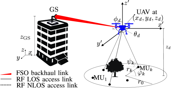
Figure 1: UAV-based communication system with FSO backhaul connection to the GS.

We consider an uplink UAV-based communication system, cf. Fig. 1, with $K$ single-antenna MUs transmitting data over RF links to a hovering UAV equipped with $N$ RF antennas and a single aperture which relays the received data over an FSO backhaul link to a GS equipped with a single PD. The position of the GS, MUs, and UAV are as follows. The GS is installed at height $z_{\mathrm{GS}}$ of a building located in the origin of the Cartesian coordinate system $(x,y,z)$, i.e., the GS has coordinates $(0,0,z_{\mathrm{GS}})$. Moreover, the $K$ MUs are randomly distributed in a cell of radius $r_{0}$ centered at $(x_{0},y_{0},0)$. The random position of $\text{MU}_{k},k\in\{1,2,\dots,K\}$, is modeled by a homogeneous Poisson point process, $\Phi$, with density $\lambda$, and is characterized by polar coordinates $(r_{k},\varphi_{k})\in\Phi$, where $0\leq r_{k}\leq r_{0}$ is the radial distance from the cell center and $\varphi_{k}\in[0,2\pi]$ is the polar angle. Furthermore, the UAV is located at position $\mathbf{p}_{d}=(x_{d},y_{d},z_{d})$ and its beam direction is determined by orientation variables $\mathbf{o}_{d}=(\theta_{d},\phi_{d})$. Consider $(x^{\prime},y^{\prime},z^{\prime})$ as a translation of the primary coordinate system, $(x,y,z)$, by vector $(x_{d},y_{d},z_{d})$, cf. Fig. 1. Then, $\phi_{d}$ is defined as the angle between the laser beam and the $z^{\prime}$-axis and $\theta_{d}$ is the angle between the $x^{\prime}$-axis and the projection of the beam onto the $x^{\prime}-y^{\prime}$ plane.

Now, the uplink transmission can be divided into two hops, the MUs-to-UAV hop and the UAV-to-GS hop. The MUs are connected via RF access links to the UAV and by assuming frequency division multiple access (FDMA), each MU’s signal is assigned to an orthogonal subchannel. Thus, the signal received at the UAV from $\text{MU}_{k}$ is given by

$$\mathbf{y}_{k}=\mathbf{h}_{k}x_{k}+\mathbf{n}_{k},$$ (1)

where $\mathbf{h}_{k}=[h_{k,1},\dots,h_{k,n},\dots,h_{k,N}]^{T}$, $h_{k,n}$ is the flat fading channel coefficient from $\text{MU}_{k}$ to the $n$-th antenna of the UAV, and $x_{k}$ is the transmit symbol of $\text{MU}_{k}$ with power $P=\mathbb{E}\{|x_{k}|^{2}\}$. Moreover, $\mathbf{n}_{k}\sim\mathcal{CN}(\mathbf{0},\zeta^{2}\mathbf{I}_{N})$ is complex circularly symmetric additive white Gaussian noise. Assuming perfect channel state information (CSI) at the UAV, the elements of the received signal vector, $\mathbf{y}_{k}$, are combined by maximum ratio combining (MRC), and the resulting signal is decoded and forwarded to the GS via the FSO link. Furthermore, the UAV can transmit and receive simultaneously due to the mutual orthogonality of the RF and FSO channels. We consider both non-BA and BA relaying at the UAV. In the former case, the UAV immediately forwards the data received from the MUs to the GS, whereas, in the latter case, the UAV can select to either receive and transmit the packets in the same time slot or to store them in its buffer and forward them in a later time slot when the FSO channel conditions are more favorable [19]. Therefore, unlike non-BA relaying, BA relaying relaxes the constraint to transmit and receive according to a predetermined schedule and the UAV can select the best strategy (transmit, receive, or transmit and receive simultaneously) based on the conditions of the MUs-to-UAV and UAV-to-GS links. Hence, BA relaying can enhance the end-to-end achievable rate at the expense of an increased delay [16], [20].

For the UAV-to-GS hop, the UAV maintains an FSO connection to the GS via a single laser aperture. Next, assuming perfect CSI at the GS and an intensity modulation and direct detection (IM/DD) FSO system, the signal intensity received at the GS’s PD can be modeled as

$$\bar{y}=g\bar{x}+\bar{n},$$ (2)

where $\bar{x}\in\mathcal{R}^{+}$ is the intensity modulated optical signal, $g$ is the scalar FSO channel coefficient, and $\bar{n}\sim\mathcal{N}(0,\rho^{2})$ is the background Gaussian shot noise obtained after removing the ambient noise [21].

II-B UAV-Based RF Channel Model

The main difference between UAV-based RF channels and the conventional channel models for satellite and terrestrial mobile communications lies in the characteristics of the LOS component. In particular, in satellite channels, the LOS path is almost always present, leading to Rician fading, whereas in urban mobile communication, due to the large number of obstacles (e.g. high rise buildings) in the environment, having an LOS path is less probable and Rayleigh fading is expected [22]. On the other hand, UAV-based communication is performed at altitudes that are between these two cases. Thus, the presence and absence of LOS links depends on the position of the UAV. This behavior was modeled in [23] and [24] via the probability of attaining an LOS link between $\text{MU}_{k}$ and the UAV which is given as follows

$$\mathrm{P}_{\mathrm{LOS},k}=\frac{1}{1+C\exp(-B\psi_{k})}\ ,$$ (3)

where $\psi_{k}=\frac{180}{\pi}\tan^{-1}(\frac{z_{d}}{r_{DM}})$ is the elevation angle between the UAV and $\text{MU}_{k}$, $r_{DM}=\big{(}(x_{d}-x_{0}-r_{k}\cos\phi_{k})^{2}+(y_{d}-y_{0}-r_{k}\sin\phi_{k})^{2}\big{)}^{1/2}$ is the radial distance between the UAV and $\text{MU}_{k}$, and $C$ and $B$ are constants whose values depend on the environment (e.g., rural, urban, and high-rise areas). Eq. (3) suggests that, at higher UAV operating altitudes, the LOS link is more likely to be present, which in turn comes at the expense of a higher path loss. Accordingly, the probability of having a non-LOS (NLOS) connection from the UAV to $\text{MU}_{k}$ is given by $\mathrm{P}_{\mathrm{NLOS},k}=1-\mathrm{P}_{\mathrm{LOS},k}$. Now, based on the LOS probability, the RF channel coefficient, $h_{k,n}$, may be either LOS or NLOS and is given by [23, 25]

$$h_{k,n}=\begin{cases}h^{p}_{k}h^{r}_{k,n}e^{j\Psi_{k,n}},&\quad\mathrm{NLOS},\\ h^{p}_{k}h^{sr}_{k,n},&\quad\mathrm{LOS},\end{cases}$$ (4)

where $h^{p}_{k}$ is the free-space path loss, and $h^{r}_{k,n}e^{j\Psi_{k,n}}$ and $h^{sr}_{k,n}$ are the Rayleigh and shadowed Rician fading coefficients, respectively. In particular, the path loss is given by $h^{p}_{k}=\frac{1}{c\sqrt{{r}_{DM}^{2}+z_{d}^{2}}}$, where $c={f\over 23.85}$ and $f$ is the center operating frequency in MHz. The NLOS scenario is characterized by the Rayleigh fading coefficient, $h^{r}_{k,n}e^{j\Psi_{k,n}}$, with power $\mathbb{E}\{\left(h^{r}_{k,n}\right)^{2}\}=\eta^{2}$ and uniformly distributed phase, $\Psi\sim\mathcal{U}(0,2\pi)$. The probability density function (pdf) of $h^{r}_{k,n}$, denoted by $f_{h^{r}_{k,n}}(x)$, is given by

$$f_{h^{r}_{k,n}}(x)={{x}\over{\eta^{2}}}e^{-{x^{2}}\over{2\eta^{2}}}.$$ (5)

Moreover, the distribution of $\varsigma=\sum\limits_{n=1}^{N}|h_{k,n}^{r}|^{2}$, which characterizes the combined signal after MRC at the UAV, is given by a chi-distribution with $2N$ degrees of freedom, i.e., $\varsigma\sim\chi^{2}(2N)$. In the LOS case, the channel is affected by both shadowing and small scale fading which is modeled via the Loo model [26], [27], [28]. In this model, the shadowed Rician fading coefficient is modeled as $h^{sr}_{k,n}\overset{\Delta}{=}h^{s}_{k}+h^{r}_{k,n}e^{j\Psi_{k,n}}$, where $h^{s}_{k}\sim\text{lognormal}(\mu,\sigma^{2})$ is the lognormal shadowed LOS component which is added to the Rayleigh scattering component. Here, the log-normal shadowed component is identical across all RF antennas of the UAV, but the small scale Rayleigh fading is independent across antennas. Unfortunately, the combination of log-normal shadowing and Ricean fading does not lend itself to a closed-form expression for the resulting distribution. Thus, as a widely accepted approximation [26], [29], the log-normal distribution is fitted to the Nakagami distribution and the shape and spread parameters of the Nakagami pdf are obtained via moment matching to the log-normal pdf as follows

$$q=\frac{1}{\exp(\frac{4\sigma^{2}}{\varepsilon^{2}})-1},\quad\omega=\exp\left({2\over\varepsilon}\left(\mu+\frac{\sigma^{2}}{\varepsilon}\right)\right),$$ (6)

where $\varepsilon=\frac{20}{\ln(10)}$ and thus, $h^{s}_{k}\sim\text{Nakagami}(q,\omega)$. Based on this approximation, the shadowed-Rician pdf is modeled in [26]. In the following Lemma, we characterize the distribution of $\tau=\sum\limits_{n=1}^{N}|h_{k,n}^{sr}|^{2}$.

Lemma 1

For the proposed Nakagami approximation of $h_{k}^{s}$, the distribution of $\tau=\sum\limits_{n=1}^{N}|h_{k,n}^{sr}|^{2}$ is given by

$$f_{{\tau}}\left(x\right)=\frac{\left(\frac{N\omega}{2q\eta^{2}}+1\right)^{-q}x^{N-1}}{2^{N}\eta^{2N}\left(N-1\right)!e^{\frac{x}{2\eta^{2}}}}\,_{1}\mathcal{F}_{1}\left(q,N;\frac{x}{2\eta^{2}+\frac{4\eta^{4}q}{N\omega}}\right),\qquad$$ (7)

where ${}_{1}F_{1}(\cdot,\cdot;\cdot)$ is the confluent hypergeometric function.

Proof:

The proof is given in Appendix A. ∎

Thus, the pdf of $\lVert{\mathbf{{h}}}_{k}\rVert^{2}=\sum\limits_{n=1}^{N}|h_{k,n}|^{2}$ is given by

$$f_{\lVert{\mathbf{{h}}}_{k}\rVert^{2}}(h)=\frac{1}{|h^{p}_{k}|^{2}}\left(f_{\tau}\left(\frac{h}{|h^{p}_{k}|^{2}}\right)\mathrm{P}_{\mathrm{NLOS},k}+f_{\varsigma}\left(\frac{h}{|h^{p}_{k}|^{2}}\right)\mathrm{P}_{\mathrm{LOS},k}\right).$$

II-C UAV-Based FSO Channel Model

The UAV-based FSO channel differs from conventional FSO channels with fixed transceivers mounted on top of buildings in the following two aspects. First, in contrast to fixed transceivers, the FSO beam of the UAV is not necessarily orthogonal to the PD plane. Second, the instability of the UAV, i.e., the random vibrations of the UAV, introduces a random power loss. Taking these effects into account, the point-to-point UAV-based FSO channel, $g$, can be modeled as follows [30, 31]

$$g=R_{s}g_{p}g_{a}g_{g},$$ (9)

where $R_{s}$, $g_{p}$, $g_{a}$, and $g_{g}$ represent the responsivity of the PD, the atmospheric loss, the atmospheric turbulence, and the geometric and misalignment loss (GML), respectively.

II-C1 Atmospheric Loss

The atmospheric loss, $g_{p}$, is due to scattering and absorption of the laser beam by atmospheric particles and is given by [30]

$$g_{p}=10^{-\frac{\kappa L}{10}},$$ (10)

where $\kappa$ is the attenuation factor, whose value depends on the weather conditions (e.g.  clear, foggy), and $L=\sqrt{x_{d}^{2}+y_{d}^{2}+(z_{d}-z_{\mathrm{GS}})^{2}}$ is the distance between the UAV and the GS.

II-C2 Atmospheric Turbulence

The atmospheric turbulence, $g_{a}$, is caused by variations of the refractive index in different layers of the atmosphere due to fluctuations in pressure and temperature. As a universal model that considers both small and large scale irradiance fluctuations, the Gamma-Gamma (GG) distribution, $g_{a}\sim\mathcal{GG}(\alpha,\beta)$, is considered. Here, $\alpha$ and $\beta$ are the small and large scale turbulence parameters, respectively, and are given by [32]

$$\alpha=\left[\exp\left({{0.49\sigma_{R}^{2}}\over{\left(1+0.18\iota^{2}+0.56\sigma_{R}^{\frac{12}{5}}\right)^{\frac{7}{6}}}}\right)-1\right]^{-1},$$

$$\beta=\left[\exp\left({{0.51\sigma_{R}^{2}\left(1+0.69\sigma_{R}^{\frac{12}{5}}\right)^{-\frac{5}{6}}}\over{\left(1+0.9\iota^{2}+0.62\iota^{2}\sigma_{R}^{\frac{12}{5}}\right)^{\frac{5}{6}}}}\right)-1\right]^{-1},\quad\quad$$ (11)

where $\iota=\left(k(2a)^{2}/4L\right)^{1/2}$, $\sigma_{R}^{2}=1.23C_{n}^{2}k^{{7}/{6}}L^{{11}/{6}}$ is the Ryotov variance, $C_{n}^{2}$ represents the index of refraction structure parameter, $k$ denotes the wave number, and $a$ is the radius of the PD. The Hufnagle-Valley (H-V) model suggests that $C_{n}^{2}$ decreases with increasing height of the UAV (up to 3 km) and is given by $C_{n}^{2}\approx C_{n}^{2}(0)\exp\left({-z_{d}\over 100}\right)$, where $C_{n}^{2}(0)$ is the ground level refraction structure parameter [7], [33]. Thus, the Ryotov variance and accordingly the scintillation variance, $\mathrm{var}\{g_{a}\}=\frac{1}{\alpha}+\frac{1}{\beta}+\frac{1}{\alpha\beta}$, depend on both the distance between the laser aperture and the PD, $L$, and the UAV operating height, $z_{d}$. Now, for conventional applications where UAVs are used to build temporary networks, short distances between the UAV and the GS, e.g., $L\leq 600\ \text{m}$, are expected. In this operating range and typical heights of $z_{d}>30\ \text{m}$, the impact of scintillation becomes very weak even in clear weather condition, i.e., $\mathrm{var}\{g_{a}\}\leq 0.15$, and hence for our analysis in Section III, we ignore the effect of turbulence, i.e., $g_{a}=\mathcal{E}\{g_{a}\}=1$ is assumed. Then, in Section IV, we use simulations to investigate the impact of this simplifying assumption on the end-to-end achievable rate of the system.

II-C3 GML

The GML, $g_{g}$, comprises the geometric loss due to the beam spread along the propagation path and the misalignment loss due to the random fluctuations of the position and orientation of the UAV. These random fluctuations are caused by different phenomena, including random air fluctuations around the UAV, internal vibrations of the UAV, and tracking errors, see [31] for a detailed discussion. Also, for the UAV-based FSO channel, the positioning of the UAV may lead to non-orthogonality between the laser beam and the PD plane, which in turn introduces an additional geometric loss. Taking the aforementioned effects into account, the GML for UAV-based FSO channels can be modeled as follows [30]

$$g_{g}=A_{0}\exp\left(-\frac{2u^{2}}{k_{g}w^{2}}\right),$$ (12)

where $u$ is the misalignment factor, $w$ is the beam width at distance $L$, $A_{0}=\text{erf}(\nu_{\mathrm{min}})\text{erf}(\nu_{\mathrm{max}})$, $k_{g}=\frac{k_{\mathrm{min}}+k_{\mathrm{max}}}{2}$, $k_{\mathrm{min}}=\frac{\sqrt{\pi}\mathrm{erf}(\nu_{\mathrm{min}})}{2\nu_{\mathrm{min}}\exp(-\nu^{2}_{\mathrm{min}})}$, $\nu_{\mathrm{min}}=\sqrt{\frac{\pi}{2}}\frac{a}{w}$, $k_{\mathrm{max}}=\frac{\sqrt{\pi}\mathrm{erf}(\nu_{\mathrm{max}})}{2\sin^{2}(\phi_{d})\cos^{2}(\theta_{d})\nu_{\mathrm{max}}\exp(-\nu^{2}_{\mathrm{max}})}$, and $\nu_{\mathrm{max}}=|\sin(\phi_{d})\cos(\theta_{d})|\nu_{\mathrm{min}}$. Here, $\text{erf}(x)=\frac{1}{\sqrt{\pi}}\int_{-x}^{x}\exp(-t^{2})\mathrm{d}t$ is the error function.

Assuming perfect tracking, i.e., $\mathbb{E}\{u\}=0$, the random variations of the position and orientation of the UAV can be characterized by a Hoyt distributed misalignment factor, i.e., $u\sim\mathcal{H}(m,\Omega)$, and accordingly, the pdf of the GML is given by [30]

$$f_{g_{g}}(g_{g}) =\frac{\varrho}{A_{0}}\left(\frac{g_{g}}{A_{0}}\right)^{\frac{(1+m^{2})\varrho}{2m}-1}$$ (13)

$$\times{I}_{0}\left(-\frac{(1-m^{2})\varrho}{2m}\ln\left(\frac{g_{g}}{A_{0}}\right)\right),\hskip 1.42262pt0\leq g_{g}\leq A_{0},\quad$$

where ${I}_{0}(\cdot)$ is the zero-order modified Bessel function of the first kind, $\varrho=\frac{(1+m^{2})k_{g}w^{2}}{4m\Omega}$, $m=\sqrt{\frac{\min\{\lambda_{1},\lambda_{2}\}}{\max\{\lambda_{1},\lambda_{2}\}}}$, $\Omega=\lambda_{1}+\lambda_{2}\$, and $\lambda_{1}$ and $\lambda_{2}$ are the eigenvalues of matrix

$$\mathbf{\Sigma}=\begin{bmatrix}\sigma_{y_{d}}^{2}+c_{1}^{2}\sigma_{x_{d}}^{2}+c_{2}^{2}\sigma_{\theta_{d}}^{2}&c_{1}c_{5}\sigma_{x_{d}}^{2}+c_{2}c_{4}\sigma_{\theta_{d}}^{2}\\ c_{1}c_{5}\sigma_{x_{d}}^{2}+c_{2}c_{4}\sigma_{\theta_{d}}^{2}&\sigma_{z_{d}}^{2}+c_{5}^{2}\sigma_{x_{d}}^{2}+c_{4}^{2}\sigma_{\theta_{d}}^{2}+c_{3}^{2}\sigma_{\phi_{d}}^{2}\end{bmatrix}.$$

(14)

Here, $\sigma^{2}_{i},i\in\{x_{d},y_{d},z_{d},\theta_{d},\phi_{d}\}$, denotes the variance of the random fluctuations of the UAV along the position and orientation variables, $c_{1}=-\tan(\theta_{d})$, $c_{2}=-\frac{x_{d}}{\cos^{2}(\theta_{d})}$, $c_{3}=\frac{x_{d}}{\sin^{2}(\phi_{d})\cos(\theta_{d})}$, $c_{4}=-\frac{x_{d}\cot(\phi_{d})\tan(\theta_{d})}{\cos(\theta_{d})}$, and $c_{5}=-\frac{\cot(\phi_{d})}{\cos(\theta_{d})}$.

Next, given (9) and (13), the pdf of the FSO channel, disregarding the atmospheric turbulence, can be modeled as

$$f_{g}(g)=\frac{1}{R_{s}g_{p}}f_{g_{g}}\left(\frac{g}{R_{s}g_{p}}\right),\quad 0\leq g\leq R_{s}g_{p}A_{0}.$$ (15)

Remark 1

To shed some light on the impact of the various system parameters on the distribution of the misalignment factor $u$, we consider special cases. Let us assume $\sigma_{x_{d}}=\sigma_{y_{d}}=\sigma_{z_{d}}=\sigma_{p}$ and $\sigma_{\theta_{d}}=\sigma_{\phi_{d}}=\sigma_{o}$. If the UAV flies in the $x$–$z$ plane, i.e., $y_{d}=\theta_{d}=0$, then we obtain $\lambda_{1}=\sigma_{p}^{2}+x_{d}^{2}\sigma_{o}^{2}$, $\lambda_{2}=\sigma_{p}^{2}(1+\cot^{2}\phi_{d})+\frac{x_{d}^{2}}{\sin^{2}\phi_{d}}\sigma_{o}^{2}$, $m={\lambda_{1}\over\lambda_{2}}$, and $\Omega=\lambda_{1}+\lambda_{2}$. Under this assumption, we consider the following special cases for $u\sim\mathcal{H}(m,\Omega)$:

• UAV flies along the $z$-axis and $x_{d}=x_{0}$: By increasing $|z_{d}-z_{\mathrm{GS}}|$, $m$ reduces and $\Omega$ increases.

• UAV flies along the $x$-axis and $z_{d}=z_{\mathrm{GS}}$: Now, $\phi_{d}=\pi/2$ and $m=1$ and decreasing $x_{d}$ reduces $\Omega$.

• UAV hovers in front of the GS: $y_{d}=0$, $z_{d}=z_{\mathrm{GS}}$, $\theta_{d}=0$, and $\phi_{d}=\frac{\pi}{2}$, then we obtain $m=1$, and $\Omega=2(\sigma_{p}^{2}+x_{d}^{2}\sigma_{o}^{2})$. In this case, the FSO beam is orthogonal to the PD plane and the misalignment factor $u$ is Rayleigh distributed.

In summary, the models for both the RF channel and the FSO channel of UAV-based relay networks differ substantially from the corresponding models for conventional relay networks without UAVs. In particular, the positioning of the UAV affects the path loss and LOS characteristics of the RF access links and the atmospheric loss of the FSO backhaul channel. Furthermore, the instability of the UAV impacts the GML of the FSO backhaul channel. In the following, we study the impact of these effects on the end-to-end achievable rate of the system.

III End-to-End Ergodic Sum Rate Analysis

In this section, the ergodic sum rate, $\mathbb{E}\{C_{\mathrm{sum}}\}$, is adopted as a metric for analyzing the end-to-end system performance. Assuming DF relaying at the UAV, the end-to-end achievable sum rate is restricted to the rate of the weaker of the two involved links as a consequence of the max-flow min-cut theorem [34]. In particular, for non-BA relaying, the achievable sum rate depends on the instantaneous fading states of both hops [18]. Thus, the non-BA ergodic sum rate, denoted by $\bar{C}^{\mathrm{NB}}_{\mathrm{sum}}$, is given by

$$\bar{C}^{\mathrm{NB}}_{\mathrm{sum}}=\mathbb{E}\{C_{\mathrm{sum}}\}=\mathbb{E}\{\min\left(C^{\mathrm{RF}},C^{\mathrm{FSO}}\right)\},$$ (16)

where $C^{\mathrm{RF}}$ and $C^{\mathrm{FSO}}$ are the instantaneous achievable rates of the RF and FSO links, respectively. In the BA scenario, the relay is equipped with buffers to store the data received from the MUs and to transmit it when the FSO channel is in a favorable state [17]. Here, for unlimited buffer sizes, the BA ergodic sum rate is given by

$$\bar{C}_{\mathrm{sum}}^{\mathrm{BA}}=\min\left(\mathbb{E}\{C^{\mathrm{RF}}\},\mathbb{E}\{C^{\mathrm{FSO}}\}\right).$$ (17)

Remark 2

Although, we assume an unlimited buffer size in (17), in practice, the buffer size is finite and hence, (17) constitutes a performance upper bound for practical BA relaying systems. However, in [17] and [18], it has been shown that the performance of BA relays with sufficiently large buffer sizes closely approaches the upper bound for unlimited buffer size.

Remark 3

Exploiting Jensen’s inequality for concave $\min$ function, $\mathbb{E}\{f(x)\}\leq f(\mathbb{E}\{x\})$, we can relate the ergodic sum rates for non-BA and BA relaying as follows

$$\bar{C}^{\mathrm{NB}}_{\mathrm{sum}}\leq\bar{C}_{\mathrm{sum}}^{\mathrm{BA}}.$$ (18)

Hence, the ergodic sum rate achieved with BA relaying is an upper bound for the ergodic sum rate of the non-BA case which suggests that buffering data is advantageous for achieving a high ergodic sum rate for the end-to-end system. Nevertheless, this gain comes at the expense of a higher end-to-end delay. Therefore, BA relaying is suitable for delay-tolerant applications.

Next, we analyze the ergodic rate for non-BA (16) and BA (17) relay UAVs for the UAV-based mixed RF-FSO channel model presented in Section II .

III-A Ergodic Rate Analysis for BA Relay UAV

The achievable rate for a BA relay UAV depends only on the individual ergodic rates of the RF and FSO channels, i.e., $\mathbb{E}\{C^{\mathrm{RF}}\}$ and $\mathbb{E}\{C^{\mathrm{FSO}}\}$ in (17). Therefore, in the following, we analyze these ergodic rates separately.

III-A1 Achievable Ergodic Sum Rate of the RF Channel

Given that the MUs employ orthogonal subchannels, the instantaneous rate of the RF channel, $C^{\mathrm{RF}}$, can be written as a summation of all MUs’ rates and is given by

$$C^{\mathrm{RF}}=W_{\mathrm{sub}}^{\mathrm{RF}}\sum\limits_{(r_{k},\phi_{k})\in\Phi}R_{k}^{\mathrm{RF}},$$ (19)

where ${W}_{\mathrm{sub}}^{\mathrm{RF}}$ is the subchannel bandwidth and $R_{k}^{\mathrm{RF}}=\log_{2}(1+\frac{P}{\zeta^{2}}\lVert\mathbf{h}_{k}\rVert^{2})$ is the achievable rate of $\text{MU}_{k}$. Now, the RF ergodic rate is determined by averaging over the random fluctuations of the shadowed Rician and Rayleigh fading in the RF channel and the random MU positions. Taking these effects into account, the ergodic sum rate of the RF channel, denoted by $\bar{C}^{\mathrm{RF}}$, is given in the following theorem.

Theorem 1

The ergodic sum rate of the RF channel is given as follows

$$\bar{C}^{\mathrm{RF}} =\mathbb{E}_{h,\Phi}\{C^{\mathrm{RF}}\}=\frac{\pi^{3}\lambda r_{0}^{2}}{4HM}W_{\mathrm{sub}}^{\mathrm{RF}}\sum_{i=1}^{H}\sum_{j=1}^{M}\sqrt{(1-x_{i}^{2})(1-y_{j}^{2})}(x_{i}+1)\big{[}\mathbb{E}_{h_{\mathrm{r}}}\{R^{\mathrm{RF}}\}+$$ (20)

$$+\left(\mathbb{E}_{h_{\mathrm{sr}}}\{R^{\mathrm{RF}}\}-\mathbb{E}_{h_{\mathrm{r}}}\{R^{\mathrm{RF}}\}\right)P_{\mathrm{LOS}}\big{]}+E_{H}+E_{M},$$

where $R^{\mathrm{RF}}=\log_{2}(1+\gamma\lVert{\mathbf{\tilde{h}}}_{k}\rVert^{2})$, ${\mathbf{\tilde{h}}}_{k}=\frac{1}{h_{k}^{p}}{\mathbf{h}}_{k}$, $\gamma=\frac{{P}}{{\zeta^{2}}c^{2}(z_{d}^{2}+\tilde{r}_{\mathrm{DM}}^{2})}$, $P_{\mathrm{LOS}}=P_{\mathrm{LOS},k}(\tilde{\psi}_{k})$ , $\tilde{\psi}_{k}=\frac{180}{\pi}\tan^{-1}(\frac{z_{d}}{\tilde{r}_{\mathrm{DM}}})$, $\tilde{r}_{\mathrm{DM}}^{2}=(x_{d}-x_{0}+\frac{r_{0}}{2}(x_{i}+1)\cos(\pi y_{j}))^{2}+(y_{d}-y_{0}+\frac{r_{0}}{2}(x_{i}+1)\sin(\pi y_{j}))^{2}$, $x_{i}=\cos\left(\frac{2i-1}{2H}\pi\right)$, $y_{j}=\cos\left(\frac{2j-1}{2M}\pi\right)$. Additionally, the ergodic rates for Rayleigh and shadowed-Rician fading are respectively given as follows

$$\mathbb{E}_{h_{\mathrm{r}}}\{R^{\mathrm{RF}}\} =\sum_{\ell=0}^{N-1}\frac{1}{(2\eta^{2}\gamma)^{\ell}}\ e^{\frac{1}{2\eta^{2}\gamma}}\ \Gamma\left(-\ell,\frac{1}{2\eta^{2}\gamma}\right),$$ (21)

$$\mathbb{E}_{h_{\mathrm{sr}}}\{R_{k}^{\mathrm{RF}}\} =\frac{\left(\frac{N\omega}{2q\eta^{2}}+1\right)^{-q}e^{-1/2\eta^{2}\gamma}}{2^{N}\eta^{2N}}\sum\limits_{n=0}^{\infty}\frac{(q)_{n}}{n!\left(2\eta^{2}+\frac{4\eta^{4}q}{N\omega}\right)^{n}\gamma^{n+N}}$$ (22)

$$\times\sum\limits_{\ell=1}^{n+N}\Gamma\left(\ell-n-N,\frac{1}{2\eta^{2}\gamma}\right)\left(2\eta^{2}\gamma\right)^{\ell},\quad$$

where $\Gamma(\cdot,\cdot)$ and $(x)_{n}$ denote incomplete Gamma function and the (rising) Pochhammer symbol, respectively [35].

Proof:

The proof is given in Appendix B. ∎

For the error terms, we have $E_{H},E_{M}\rightarrow 0$ as $H$ and $M$ increase. In Section IV, we will show that even for small values of $H$ and $M$ (e.g., $H=M=10$), (20) yields accurate results. Theorem 1 explicitly reveals the dependence of the ergodic sum rate of the RF channel on the position of the UAV via parameters $\gamma$ and $P_{\mathrm{LOS}}$. In particular, by moving the UAV upwards (larger $z_{d}$) or towards the GS (smaller $x_{d}$ or $y_{d}$), $\gamma$ and accordingly both ergodic sum rate terms, $\mathbb{E}_{h_{\mathrm{sr}}}\{R^{\mathrm{RF}}\}$ and $\mathbb{E}_{h_{\mathrm{r}}}\{R^{\mathrm{RF}}\}$, decrease. Given the LOS path in $h_{sr}$, for the same multipath power $\eta^{2}$, the ergodic sum rate for shadowed Rician fading is always larger than that for Rayleigh fading, and the term $\mathbb{E}_{h_{\mathrm{sr}}}\{R^{\mathrm{RF}}\}-\mathbb{E}_{h_{\mathrm{r}}}\{R^{\mathrm{RF}}\}$ decreases by moving the UAV further from the cell center. On the other hand, the LOS probability, $P_{\mathrm{LOS}}$, increases for larger $z_{d}$ and decreases for smaller $x_{d}$ and $y_{d}$. Therefore, the ergodic sum rate of the RF channel always degrades if the UAV moves away from the cell center towards the GS (smaller $x_{d}$ or $y_{d}$), but for vertical movement of the UAV (larger $z_{d}$), there is a trade-off between the LOS probability and the path loss. Thus, the positioning of the UAV plays an important role for the achievable rate of the RF channel.

III-A2 Achievable Ergodic Rate of the FSO Channel

In the second hop, for an average power constraint, $\bar{p}$, the achievable rate of an IM/DD FSO system is given by [21]

$$C^{\mathrm{FSO}}=\frac{1}{2}W^{\mathrm{FSO}}\log_{2}\left(1+\frac{e\bar{p}^{2}}{2\pi\rho^{2}}g^{2}\right),$$ (23)

where $W^{\mathrm{FSO}}$ denotes the FSO bandwidth. Unfortunately, the ergodic rate of the FSO system cannot be computed in closed form for the entire range of signal-to-noise ratios (SNRs). In fact, the expected value of (23) w.r.t. the squared Hoyt variable, $u^{2}$, i.e., $\bar{C}^{\mathrm{FSO}}=\frac{W^{\mathrm{FSO}}(1+m^{2})}{4m\Omega}$ $\times\int\limits_{0}^{\infty}\log_{2}\left(\!1+\bar{\gamma}^{2}e^{\!-\frac{4x}{k_{g}w^{2}}}\right)e^{-\frac{(1+m^{2})^{2}x}{4m^{2}\Omega}}I_{0}\left(\frac{(1-m^{4})x}{4m^{2}\Omega}\right)\mathrm{d}x$, does not have a closed-form solution and can only be obtained numerically. Nevertheless, the following theorem presents the ergodic rate for low and high SNRs.

Theorem 2

The ergodic rate of the FSO system for the low and high SNR regimes, i.e., $\bar{\gamma}<1$ and $\bar{\gamma}\gg 1$, respectively, is given by

$$\bar{C}^{\mathrm{FSO}}_{\mathrm{low}} =\frac{W^{\mathrm{FSO}}}{\ln(2)}\sum_{\ell=1}^{\infty}\frac{(-1)^{\ell+1}\left(\bar{\gamma}\right)^{2\ell}}{\ell\sqrt{\frac{(4\ell)^{2}}{\varrho^{2}}+4\left(1+\frac{8\ell\Omega}{k_{g}w^{2}}\right)}},\qquad$$ (24a)

$$\bar{C}^{\mathrm{FSO}}_{\mathrm{high}} =\frac{W^{\mathrm{FSO}}}{2}\left(\log_{2}(\bar{\gamma}^{2})-\frac{4\Omega}{\ln(2)k_{g}w^{2}}\right),\qquad$$ (25a)

where $\bar{\gamma}=R_{s}g_{p}A_{0}\left(\frac{e\bar{p}^{2}}{2\pi\rho^{2}}\right)^{1\over 2}$.

Proof:

Please refer to Appendix C. ∎

As will be shown in Section IV, (24a) yields an accurate approximation even if the number of summation terms is limited to only $5$. Here, variables $w,\Omega,\varrho,g_{p}$, and $A_{0}$ are dependent on the position and orientation parameters of the UAV, namely $\mathbf{p}_{d}$ and $\mathbf{o}_{d}$. Theorem 2 reveals that the ergodic rate of the FSO channel depends on the positioning of the UAV via $g_{p}$, $w$, $A_{0}$ and on the instability of the UAV via Hoyt parameters $m$ and $\Omega$.

Remark 4

To gain some insights, let us consider the case where the UAV changes only its altitude and flies along the $x$-axis. When the UAV is located at the same height as the GS, the beam is orthogonal to the PD plane. Recall from Remark 1 that in this case, $m=1$, $\Omega$ assumes its minimum value and since, the beam has the maximum possible footprint on the PD, $A_{0}$ takes its maximum value. Then, if the UAV moves to higher or lower altitudes than the GS, $m$ and $A_{0}$ decrease, $\Omega$ increases, and accordingly, the GML increases. Moreover, due to the larger distance between the UAV and the GS, the additional atmospheric loss increases which further deteriorates the FSO channel. Hence, $\bar{\gamma}$ decreases which in turn degrades the ergodic rate of the FSO channel. Thus, the UAV’s position and its (in)stability crucially affect the ergodic rate of the FSO channel via $\bar{\gamma}$ and parameters $m$ and $\Omega$, respectively.

Finally, the BA ergodic sum rate in (17) is given by

$$\bar{C}_{\mathrm{low}}^{\mathrm{BA}} =\min\left(\bar{C}^{\mathrm{RF}},\bar{C}^{\mathrm{FSO}}_{\mathrm{low}}\right),\quad\bar{\gamma}<1,\qquad$$ (26a)

$$\bar{C}_{\mathrm{high}}^{\mathrm{BA}} =\min\left(\bar{C}^{\mathrm{RF}},\bar{C}^{\mathrm{FSO}}_{\mathrm{high}}\right),\quad\bar{\gamma}\gg 1,\qquad$$ (27a)

where $\bar{C}^{\mathrm{RF}}$, $\bar{C}^{\mathrm{FSO}}_{\mathrm{low}}$, and $\bar{C}^{\mathrm{FSO}}_{\mathrm{high}}$ are given by (20), (24a), and (25a), respectively. Eq. (26a) illustrates the inherent trade-off between the ergodic rates of the RF and FSO channels which are dependent on the position and the instability of the hovering UAV. The position of the UAV affects the LOS probability, path loss, and geometric loss of the RF and FSO channels and the instability of the UAV influences the misalignment loss of the FSO channel. Considering these effects, in Section IV, the expression in (26a) is employed to optimize the positioning of the BA UAV for maximization of the end-to-end system performance.

III-B Ergodic Rate Analysis for Non-BA Relay UAV

In this section, we assume that the UAV is not equipped with a buffer and the instantaneous rate in each channel hop determines the system’s end-to-end rate. The non-BA ergodic rate in (16) can be written as [36]

$$\bar{C}^{\mathrm{NB}}_{\mathrm{sum}}=\int_{t>0}\mathrm{Pr}(x>t)\ \mathrm{d}t=\int_{0}^{\infty}(1-F_{x}(t))\ \mathrm{d}t,$$ (28)

where $x=\min\left(C^{\mathrm{RF}},C^{\mathrm{FSO}}\right)$. Here, the cumulative distribution function (CDF), $F_{x}(x)$, depends on the CDF of both the RF and FSO channels as follows

$$F_{x}(x)=1-(1-F_{C^{\mathrm{RF}}}(x))(1-F_{C^{\mathrm{FSO}}}(x)).$$ (29)

Here, $F_{C^{\mathrm{RF}}}(x)=F_{R_{1}^{\mathrm{RF}}}(\tilde{x})*\dots*F_{R_{K}^{\mathrm{RF}}}(\tilde{x})$, where $F_{R_{k}^{\mathrm{RF}}}(\tilde{x})$ denotes the CDF of the sum rate of $\text{MU}_{k}$ and $\tilde{x}=\frac{x}{W_{\mathrm{sub}}^{\mathrm{RF}}}$. Particularly, $F_{R_{k}^{\mathrm{RF}}}(\tilde{x})$ is the summation of the CDFs of the sum of a squared shadowed Rician RV and a squared Rayleigh RV. Thus, $F_{C^{\mathrm{RF}}}(u)$ does not lend itself to a closed-form expression. To cope with this issue, the following lemma is proposed.

Lemma 2

Assuming the number of MUs is sufficiently large, $\lim\limits_{K\rightarrow\infty}{C}^{\mathrm{RF}}=\bar{C}^{\mathrm{RF}}$, then the ergodic rate for the non-BA relay UAV is given by

$$\lim\limits {}_{K\rightarrow\infty}\bar{C}^{\mathrm{NB}}_{\mathrm{sum}}=$$ (30)

$$\mathbb{E}_{g}\{\!C^{\mathrm{FSO}}|C^{\mathrm{FSO}}\leq\bar{C}^{\mathrm{RF}}\!\}+\bar{C}^{\mathrm{RF}}(1-F_{C^{\mathrm{FSO}}}(\bar{C}^{\mathrm{RF}})).\qquad$$

Proof:

Please refer to Appendix D. ∎

In Section IV, we provide simulation results to confirm that even for comparatively small numbers of MUs (e.g., $\bar{K}=\mathbb{E}\{K\}\geq 50$), (30) is an accurate approximation. Based on (30), two terms are needed to analyze the non-BA ergodic rate, namely $F_{C^{\mathrm{FSO}}}(\bar{C}^{\mathrm{RF}})$ and $\mathbb{E}_{g}\{C^{\mathrm{FSO}}|C^{\mathrm{FSO}}\leq\bar{C}^{\mathrm{RF}}\}$, which are determined in the following. The CDF of the achievable rate of the FSO channel is a function of the CDF of a squared Hoyt distributed RV, $u^{2}$, [37] and is given by

$$F_{C^{\mathrm{FSO}}}(x) =1-\frac{2m}{1+m^{2}}\,\textrm{Ie}\left(\!\frac{1-m^{2}}{1+m^{2}},\frac{(1+m^{2})^{2}}{4m^{2}\Omega}\chi(x)\!\right),\quad\chi(x)\geq 0,\qquad$$ (31)

where $\chi(x)=\frac{-k_{g}w^{2}}{4}\ln\left(\frac{1}{\bar{\gamma}^{2}}\left({e^{\frac{2\ln(2)x}{W^{\mathrm{FSO}}}}-1}\right)\right),0\leq x\leq\frac{W^{\mathrm{FSO}}}{2}\log_{2}(\bar{\gamma}+1)$, and the Rice-Ie function is defined as

$$\textrm{Ie}(v,t)=\frac{1}{\sqrt{1-v^{2}}}\left[{Q(\sqrt{v_{1}t},\sqrt{v_{2}t})-Q(\sqrt{v_{2}t},\sqrt{v_{1}t})}\right],\qquad$$ (32)

where $v_{1}=1+\sqrt{1-v^{2}}$, $v_{2}=1-\sqrt{1-v^{2}}$, and $Q(\cdot,\cdot)$ denotes the Marcum $Q$-function. For the special case, where the FSO beam is orthogonal to the PD plane, i.e., $m=1$, (31) becomes the CDF of an exponential distribution. This result is in line with [30], where for an orthogonal beam, misalignment factor $u$ was shown to be Rayleigh distributed, which implies that $u^{2}$ is exponentially distributed.

Theorem 3

For low and high SNRs, the average FSO rate, conditioned on the FSO channel being the instantaneous bottleneck of the end-to-end achievable rate, is given by

$$\mathbb{E}^{\mathrm{low}}_{g}\{C^{\mathrm{FSO}}|C^{\mathrm{FSO}}\leq\bar{C}^{\mathrm{RF}}\}=\frac{W^{\mathrm{FSO}}(1+m^{2})}{4\pi\ln(2)m\Omega}\sum_{\ell=1}^{\infty}\frac{(-\bar{\gamma}^{2})^{\ell}}{\ell}e^{-a\chi(\bar{C}^{\mathrm{RF}})}\int\limits_{0}^{\pi}\frac{e^{b\chi(\bar{C}^{\mathrm{RF}})\cos t}}{a-b\cos t}\mathrm{d}t,\quad\bar{\gamma}<1,\qquad$$ (33a)

$$\mathbb{E}^{\mathrm{high}}_{g}\{C^{\mathrm{FSO}}|C^{\mathrm{FSO}}\leq\bar{C}^{\mathrm{RF}}\} =\frac{W^{\mathrm{FSO}}}{2\ln(2)}\Big{(}\ln\left(\bar{\gamma}^{2}\right)F_{C^{\mathrm{FSO}}}(\bar{C}^{\mathrm{RF}})-\frac{2(1+m^{2})e^{-\delta\chi(\bar{C}^{\mathrm{RF}})}}{\pi k_{g}w^{2}m\Omega}$$ (34a)

$$\times\int\limits_{0}^{\pi}\frac{e^{b\chi(\bar{C}^{\mathrm{RF}})\cos t}(1+\chi(\bar{C}^{\mathrm{RF}})(\delta-b\cos t))}{(\delta-b\cos t)^{2}}\mathrm{d}t\Big{)},\quad\bar{\gamma}\gg 1,$$

where $a=\frac{4\ell}{k_{g}w^{2}}+\delta$, $b=\frac{(1-m^{4})}{4m^{2}\Omega}$, and $\delta=\frac{(1+m^{2})^{2}}{4m^{2}\Omega}$.

Proof:

The proof is given in Appendix E. ∎

In Section IV, we will show that the infinite sum in (33a) converges to the exact result if only the first $5$ terms are used. Moreover, (33a) and (34a) include finite-range integrals that can be calculated numerically. Furthermore, it can be shown that Theorem 2 is a special case of Theorem 3. In particular, if the RF channel always supports a higher achievable rate than the FSO channel, or equivalently if the conditions in the expected values in (33a) and (34a) are always fulfilled by assuming $\bar{C}^{\mathrm{RF}}\rightarrow\infty$, then (33a) approaches the ergodic rate of the FSO channel in Theorem 2.

In summary, we can closely approximate the ergodic sum rate for UAVs employing non-BA relaying by substituting (20), (31), (33a), and (34a) into (30) to obtain

$$\lim\limits_{K\rightarrow\infty}\bar{C}^{\mathrm{NB}}_{\mathrm{low}} =\mathbb{E}^{\mathrm{low}}_{g}\{C^{\mathrm{FSO}}|C^{\mathrm{FSO}}\leq\bar{C}^{\mathrm{RF}}\}+\bar{C}^{\mathrm{RF}}(1-F_{C^{\mathrm{FSO}}}(\bar{C}^{\mathrm{RF}})),\quad\bar{\gamma}<1,\qquad$$ (35a)

$$\lim\limits_{K\rightarrow\infty}\bar{C}^{\mathrm{NB}}_{\mathrm{high}} =\mathbb{E}^{\mathrm{high}}_{g}\{C^{\mathrm{FSO}}|C^{\mathrm{FSO}}\leq\bar{C}^{\mathrm{RF}}\}+\bar{C}^{\mathrm{RF}}(1-F_{C^{\mathrm{FSO}}}(\bar{C}^{\mathrm{RF}})),\quad\bar{\gamma}\gg 1.\qquad$$ (36a)

Eq. (35a) together with (20), (31), and (33a) reveals that the ergodic rate for non-BA relaying at the UAV crucially depends on the position and the instability of the UAV via $\bar{\gamma}$, ${\gamma}$, $m$, and $\Omega$. In Section IV, we investigate the accuracy of (35a) for small numbers of MUs and employ this expression to study the performance of non-BA relaying UAV-based communications networks and to optimize the position of the non-BA relaying UAV.

IV Simulation Results

In this section, first we use simulation results to validate the analytical results in (26a) and (35a) for BA and non-BA relay UAVs, respectively. Then, we investigate the impact of the positioning of the UAV on the system performance. Finally, we study the inherent trade-offs in the considered network and the impact of different system and channel parameters on the end-to-end ergodic sum rate.

For the considered system and channel models, the parameter values provided in Table I are adopted, unless specified otherwise. The MUs are homogeneous Poisson distributed with density $\lambda=0.008$ $\mathrm{MUs}/\mathrm{m^{2}}$ over a circular area with radius $r_{0}=50\$m, where the center of this area is located at $(x_{0},y_{0},0)=(600,0,0)$ m. We allocate $W^{\mathrm{RF}}_{\mathrm{sub}}=\frac{W^{\mathrm{RF}}}{\bar{K}}=79.4\ \mathrm{kHz}$ to each MU where $W^{\mathrm{RF}}=5\ \mathrm{MHz}$ and $\bar{K}=\mathbb{E}\{K\}=\lambda\pi r_{0}^{2}=63.3$. The GS is located at a height of $z_{\mathrm{GS}}=100$ m above the origin of the Cartesian coordinate system.

TABLE I: System and Channel Parameters [2], [24], [30].

FSO Channel Parameters	Symbol	Value
FSO bandwidth	$W^{\text{FSO}}$	$1\ \mathrm{GHz}$
Aperture radius	$a$	$10\ \mathrm{cm}$
Beam waist radius	$w_{0}$	$0.25\ \mathrm{mm}$
Responsivity	$R$	$0.5$
Index of refraction structure parameter	$C^{2}_{n}(0)$	$1.7\times 10^{-14}\ \mathrm{m}^{2/3}$
Tx power	$\bar{p}$	$0.1\ \mathrm{mW}$
Noise variance	$\rho^{2}$	$10^{-14}\ \mathrm{A}^{2}/\mathrm{Hz}$
Attenuation factor	$\kappa$	$16.8\times 10^{-3}\frac{\mathrm{dB}}{m}$
GS height	$z_{\mathrm{GS}}$	$100\ \mathrm{m}$
RF Channel Parameters
Operating frequency	$f$	$2\ \mathrm{GHz}$
RF bandwidth	$W^{\text{RF}}_{\mathrm{sub}}$	$79\ \mathrm{kHz}$
User transmit power	$P$	$20\ \mathrm{dBm}$
Multipath power	$\eta^{2}$	$22\ \mathrm{dBm}$
Noise power spectral density	$N_{0}$	$-114\ \mathrm{dBm}/\mathrm{MHz}$
Shadowing parameters	$(\mu,\sigma^{2})$	$(0,3)\ \mathrm{dB}$
Radius of MUs’ area	$r_{0}$	$50\ \mathrm{m}$
LOS probability	$(B,C)$	$(0.136,60.69)$
MU density	$\lambda$	$0.008$ $\mathrm{MUs}/\mathrm{m}^{2}$
UAV Parameters
Position STD	$\sigma_{p}$	$1\ \mathrm{cm}$
Orientation STD	$\sigma_{o}$	$0.3\ \mathrm{mrad}$
Number of RF antennas	$N$	$2$
Initial Position	$(x_{0},y_{0},z_{d0})$	$(600,0,30)\ \mathrm{m}$

For the RF channel, the two state channel model in (4) with LOS and NLOS states is adopted. In the NLOS and LOS states, Rayleigh fading with multipath power $\eta^{2}$ and shadowed Rician fading with lognormal shadowing parameters $(\mu,\sigma)$ are assumed, respectively. The LOS probability parameters, $(B,C)$, in (3) are chosen for an urban environment [24]. For the FSO channel, simulations with and without GG atmospheric turbulence were conducted. The atmospheric loss and GML are incorporated according to (9). The UAV is assumed to be able to track the PD with zero mean misalignment factor, $u$, and the UAV’s instability in the hovering state is accounted for by the position and orientation standard deviations (STD) $\sigma_{o}=0.3\ \mathrm{mrad}$ and $\sigma_{p}=1\ \mathrm{cm}$, respectively. Given the above assumptions and parameters, we obtained the results reported in this section by averaging over $10^{6}$ realizations of the RF and FSO channels as well as of the MU distributions.

IV-A Validation of Analytical Results

In this subsection, we investigate the accuracy of the following assumptions and approximations made in our analysis: 1) ignorance of the atmospheric turbulence, $g_{a}$, in the FSO channel, 2) accuracy of $\bar{C}^{\mathrm{NB}}_{\mathrm{sum}}$ in (30) for finite $K$, 3) fitting of the lognormal shadowing to Nakagami fading in (7), 4) Gaussian-Chebyshev Quadrature (GCQ) numerical approximation in (20), 5) Taylor series expansions in (26a) and (35a). Furthermore, we confirm our analytical results in (26a) and (35a) for low and high SNR scenarios.

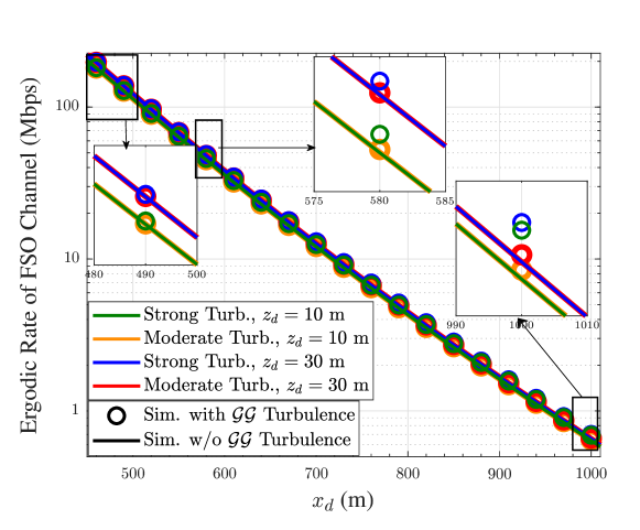
Figure 2: Ergodic rate of the FSO channel vs. distance of the UAV from the GS under strong ($C_{n}^{2}(0)=10^{-13}$) and moderate ($C_{n}^{2}(0)=10^{-14}$) turbulence conditions and UAV altitudes of $z_{d}=10,30$ m.

In Section II-C2, we argued that the atmospheric turbulence factor, $g_{a}$, can be ignored when the UAV flies at typical operating altitudes and for small distances from the GS. Fig. 2 investigates the accuracy of this approximation by comparing the ergodic rates of the FSO channel with and without GG fading as functions of the distance between the UAV and the GS. Here, strong and moderate turbulence conditions, which have different ground level refraction structure parameters, $C_{n}^{2}(0)$, and different UAV operating altitudes, $z_{d}$, are considered. Fig. 2 suggests that at a distance of $1$ km, the gap between the curves with and without GG fading at altitudes of $10$ m and $30$ m is respectively about $7\%$ and $5\%$ for strong turbulence. The smaller gap for the higher altitude is due to the H-V model since $C_{n}^{2}(z_{d})$ decreases if $z_{d}$ increases. Furthermore, Fig. 2 shows that the gap between the ergodic rates with and without GG fading vanishes for small distances. Considering the dependence of parameters $\alpha$ and $\beta$ on the distance in (II-C2), the impact of atmospheric turbulence decreases for shorter distances. Since the practical operating range of UAVs is expected to be within one kilometer of the GS and its typical operating altitude is expected to be above $30$ m, the impact of atmospheric turbulence can be savely ignored.

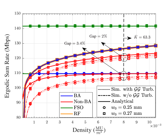
Figure 3: Ergodic sum rate vs. MU density for BA and non-BA relay UAVs for $W_{\mathrm{RF}}^{\mathrm{sub}}=\frac{W_{\mathrm{RF}}}{\bar{K}}$ and $\bar{K}=\lambda\pi r_{0}^{2}$. The analytical results for the FSO channel, the RF channel, BA relaying, and non-BA relaying are obtained from (24a), (20), (35a), and (26a), respectively.

Fig. 3 shows the ergodic sum rate versus MU density, $\lambda$, for FSO beam waists of $w_{0}=w({L=0})=0.25$ mm and $0.27$ mm. Here, the subchannel bandwidth assigned to the MUs is proportional to the average number of MUs and the total bandwidth is kept constant for all values of $\lambda$, i.e., $W^{\mathrm{RF}}_{\mathrm{sub}}=\frac{W^{\mathrm{RF}}}{\bar{K}}$ where $W^{\mathrm{RF}}=5\mathrm{MHz}$ and $\bar{K}=\mathbb{E}\{K\}=\lambda\pi r_{0}^{2}$. Fig. 3 confirms that not taking into account $g_{a}$ does not affect the ergodic rate of the FSO channel and yields accurate results for BA relaying. For non-BA relaying, there is a small gap of about $1\%$ between the simulation results with and without GG fading. Furthermore, in the non-BA case, the simulation results are upper bounded by the analytical results obtained from (35a). However, for sufficiently large numbers of MUs or equivalently for sufficiently high MU densities, the instantaneous sum rate of the RF channel approaches the ergodic sum rate of the RF channel (see Lemma 2) and hence, the gap between numerical and analytical results vanishes also for non-BA relaying. Fig. 3 suggests that even for a relatively small number of MUs, this gap is small. For example, for $\lambda=0.008$ or equivalently $\bar{K}=63.3\ \mathrm{MU}$, the gap is only about $2\%$ and $3.4\%$ for $w_{0}=0.25$ mm and $w_{0}=0.27$ mm, respectively.

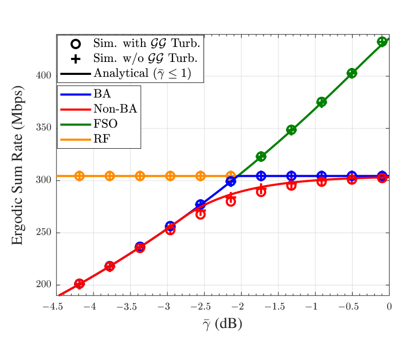
Figure 4: Ergodic sum rate of RF and FSO channels and BA and non-BA relaying vs. SNR of FSO channel in the low SNR regime. Analytical results for FSO channel (24a), RF channel (20), BA relaying (26a), and non-BA relaying (35a) are shown. $r_{0}=80$ m.

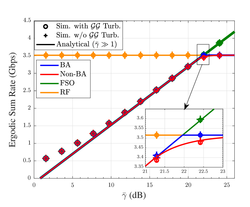
Figure 5: Ergodic sum rate of RF and FSO channels and BA and non-BA relaying vs. SNR of FSO channel in the high SNR regime. Analytical results for FSO channel (25a), RF channel (20), BA relaying (27a), and non-BA relaying (36a) are shown. $r_{0}=300$ m.

In Figs. 5 and 5, we compare the analytical and simulation results for low and high SNRs, respectively, and make the following observations. 1) Although we consider only the first five terms in the summation of the Taylor series in (24a), the analytical ergodic rate of the FSO channel perfectly matches the corresponding simulation results. 2) The analytical ergodic sum rate of the RF channel, where we consider only 10 terms ($H=M=10$) for the GCQ approximation in (20), agrees well with the simulation results. This also confirms that the approximation of the log-normal distribution by Nakagami fading for shadowed Rician fading in (7) is justified. Overall, we conclude that the analytical ergodic sum rate expressions for BA and non-BA relaying UAVs in (27a) and (36a), respectively, are accurate.

IV-B Impact of Positioning of the UAV

Next, we investigate the impact of the placement of the UAV on the end-to-end ergodic rate. Fig. 6 depicts the ergodic sum rate as a function of the UAV’s altitude, where the UAV is located at the center of the MUs’ area. Here, the ergodic sum rate of the RF link suggests an optimum altitude of $30\ \mathrm{m}$, which is a direct consequence of the trade-off between the probability of a LOS link and the value of the path loss. Furthermore, the ergodic rate of the FSO channel reaches its maximum value at a height of $100$ m; the same height at which the PD is installed. At this altitude, the FSO beam is orthogonal w.r.t. the PD plane and accordingly, the GML, $g_{g}$, and the atmospheric loss, $g_{p}$, assume their respective minimum values, cf. Remark 4. The optimum height for BA relaying, $z_{d}^{\mathrm{BA}}$, depends on the altitude at which the ergodic sum rate curves of both links intersect, i.e., $\bar{C}^{\mathrm{RF}}=\bar{C}^{\mathrm{FSO}}$ and is marked by $\davidsstar$ in Fig. 6. On the other hand, for non-BA relaying, the gap between the analytical and simulation results is only $2\%$ and the altitudes that maximize the respective curves, $z_{d}^{\mathrm{NB}}$, are only 8 m apart. Because of the benefits of buffering, BA relaying yields a higher ergodic sum rate than non-BA relaying.

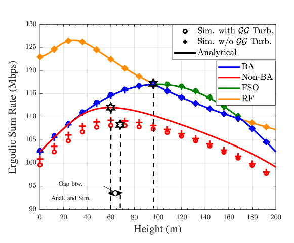
Figure 6: Ergodic sum rate vs. UAV altitude ($z_{d}$) when the UAV hovers above the center of the MUs’ area. Analytical results for the FSO channel (24a), the RF channel (20), BA relaying (26a), non-BA relaying (35a) are shown.

In Fig. 7, the UAV operates at a height of $30$ m and moves along the $x$-axis from the cell center towards the GS. By reducing the distance to the GS, the ergodic rate of the FSO channel drastically increases, due to the exponential reduction of the atmospheric loss. On the other hand, the ergodic rate of the RF channel decreases due to the larger path loss and the smaller LOS probability caused by the smaller elevation angle in (3). Consequently, farther from the cell center, the RF channel is the performance bottleneck and the ergodic rates of both BA and non-BA relaying approach the ergodic sum rate of the RF channel. On the other hand, when the UAV is farther from the GS, the FSO channel limits the performance of both types of relaying. For BA relaying, the intersection of the RF and FSO ergodic sum rate curves corresponds to the optimal position of the UAV at $11$ m, and analysis and simulations yield the same value. On the other hand, comparing the analytical and simulated ergodic rates for non-BA relaying reveals a gap of only $1\%$. The maxima of the corresponding curves are 5 m apart, which has little impact on the optimal value since the ergodic rate curves are flat around the maxima. Figs. 6 and 7 confirm that the optimal positioning of the relay depends on the parameters of the RF and FSO channels as well as the type of relaying.

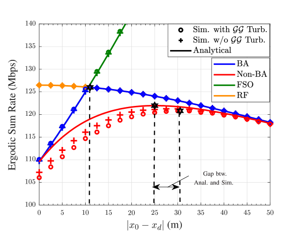
Figure 7: Ergodic sum rate vs. UAV’s distance from the center of the MUs’ cell. UAV moves along x-axis. Analytical results for the FSO channel (24a), the RF channel (20), BA relaying (26a), non-BA relaying (35a) are shown.

IV-C Impact of System Parameters

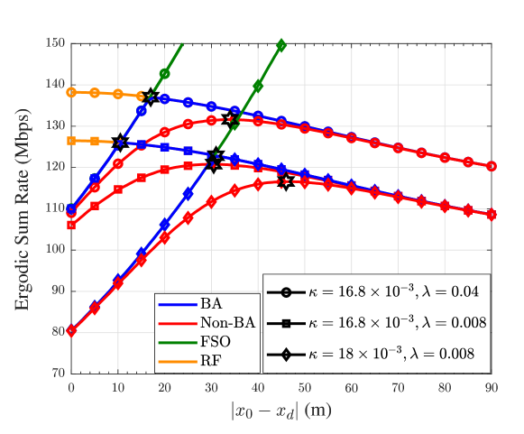
Figure 8: Simulated ergodic sum rate vs. UAV’s distance from cell center for attenuation factors $\kappa=[16.8,18]\times 10^{-3}\frac{\mathrm{dB}}{m}$ and MU densities $\lambda=[0.008,0.04]\ \mathrm{MUs}/\mathrm{m}^{2}$.

In this subsection, we investigate the impact of the weather-dependent FSO attenuation factor, $\kappa$, and the density of the MUs, $\lambda$, on the end-to-end system performance. Here, for clarity of presentation, we only show simulated ergodic sum rates.

Fig. 8 shows the impact of different weather-dependent FSO attenuation factors, i.e., $\kappa=[16.8,18]\times 10^{-3}\frac{\mathrm{dB}}{m}$, and different MU densities, i.e., $\lambda=[0.008,0.04]\ {\mathrm{MU}}/{\mathrm{m}^{2}}$, on the system performance and the optimum position of the UAV. As expected, for larger attenuation factors, the ergodic rate of the FSO link degrades due to the larger atmospheric loss. Thus, for larger $\kappa$, for both BA and non-BA relay UAVs, a position closer to the GS (i.e., larger $|x_{0}-x_{d}|$) is preferable in order to compensate for the reduced ergodic rate in the FSO link. Furthermore, for higher densities $\lambda$, the bandwidth available for each MU decreases, and accordingly, the $\mathrm{SNR}=\frac{P}{N_{0}W_{\mathrm{sub}}^{\mathrm{RF}}}$ for each MU increases. Thus, the ergodic rate of the RF channel improves. Although, a larger number of MUs does not affect the ergodic rate of the FSO channel, the FSO backhaul has to support the increased rate of the RF channel. Therefore, for larger MU densities, for both BA and non-BA relaying the UAV benefits from moving towards the GS (i.e., increasing $|x_{0}-x_{d}|$) to improve the quality of its backhaul channel.

V Conclusions

In this paper, the end-to-end performance of a UAV-based communication system, where a relay UAV connects MUs via RF access links to a GS via an FSO backhaul link, was analyzed in terms of the ergodic sum rate. The UAV’s characteristics including its relative position w.r.t. the GS and the MUs and its (in)stability in the hovering state were taken into account in the adopted RF and FSO channel models. In particular, the probability of attaining an LOS path in the RF channel and the GML in the FSO channel were accounted for. Furthermore, to address the application dependent sensitivity to delay, both BA and non-BA relay UAVs were investigated. Exact and approximate expressions for the ergodic sum rate were derived for BA and non-BA relay UAVs, respectively. We validated the accuracy of the obtained analytical result and investigated the trade-offs affecting the optimum position of BA and non-BA relay UAVs. Our results revealed that the impact of atmospheric turbulence on the quality of the FSO channel can be ignored for practical UAV-GS distances of less than 1 km. Furthermore, the derived approximate analytical expression for the ergodic sum rate for non-BA relays was shown to approach the corresponding simulation results for sufficiently large numbers of MUs. Moreover, our simulations revealed that the random variations of the FSO channel caused by the UAV’s instability can be mitigated by BA relaying which results in larger achievable ergodic sum rate compared to non-BA relaying at the expense of introducing an additional delay into the system. Our results also show that when the weather conditions get worse and accordingly the atmospheric loss in the backhaul channel increases, the UAV prefers a position closer to the GS to improve the quality of the backhaul channel. Furthermore, for higher MU densities and the resulting larger amounts of data received via the RF access channel, the end-to-end performance can be improved if the UAV moves closer to the GS in order to enhance the backhaul link quality. Considering our simulation and analytical results, we conclude that the specific properties of both the FSO backhaul and RF access channels have to be simultaneously taken into account for performance evaluation and optimization of UAV-based communication networks employing mixed RF-FSO channels.

Appendix A Proof of Lemma 1

Given that $h_{k,n}^{sr}=h_{k}^{s}+h^{r}_{k,n}e^{j\Psi_{k,n}}$ is a Rician distributed RV with Nakagami distributed parameter $h_{k}^{s}\sim\mathrm{Nakagami}(q,\omega)$, the conditional distribution of $\sqrt{\tau}$ is given by a non-central chi distribution as follows

$$f_{\sqrt{\tau}|h_{k}^{s}}\left(x\right)=\frac{x^{N}}{\eta^{2}\varkappa^{N-1}}\exp\left(-\frac{x^{2}+\varkappa^{2}}{2\eta^{2}}\right)I_{N-1}\left(\frac{\varkappa x}{\eta^{2}}\right),\qquad$$ (37)

where $\varkappa^{2}=\sum\limits_{n=1}^{N}(h^{s}_{k})^{2}=N(h^{s}_{k})^{2}$. Since $h^{s}_{k}\sim\mathrm{Nakagami}\left(q,\omega\right)$, thus, $(h^{s}_{k})^{2}$ is a Gamma distributed RV and the pdf of $\varkappa^{2}$ is given by

$$f_{\varkappa^{2}}\left(y\right)=\frac{q^{q}}{\left(\omega N\right)^{q}\Gamma(q)}y^{q-1}e^{-qy/\left(N\omega\right)}.\quad$$ (38)

Then, we can obtain the unconditional distribution of $\sqrt{\tau}$ as $f_{\sqrt{\tau}}\left(x\right)=\int\limits_{0}^{\infty}f_{\sqrt{\tau}|h_{k}^{s}}\left(x\right)f_{\varkappa^{2}}\left(y\right)\mathrm{d}y$. To solve this integral, we exploit $I_{v}(x)=\frac{(x/2)^{v}}{v!}\,_{0}\mathcal{F}_{1}\left(v+1,x^{2}/4\right)$ [39] and [35, Eq. (7.522-9)], where ${}_{0}\mathcal{F}_{1}\left(\cdot,\cdot\right)$ is the confluent hypergeometric function. Thus, the pdf of $\sqrt{\tau}$ is given by

$$f_{\sqrt{\tau}}\left(x\right)=\frac{2\left(\frac{N\omega}{2q\eta^{2}}+1\right)^{-q}x^{2N-1}}{(2\eta^{2})^{N}\left(N-1\right)!e^{\frac{x^{2}}{2\eta^{2}}}}\,_{1}\mathcal{F}_{1}\left(q,N;\frac{x^{2}}{2\eta^{2}+\frac{4\eta^{4}q}{N\omega}}\right).$$

Then, using the relation $f_{\tau}(x)=\frac{1}{2\sqrt{x}}f_{\sqrt{\tau}}(\sqrt{x})$, the pdf of $\tau$ is obtained as in (7) and this concludes the proof.

Appendix B Proof of Theorem 1

First, the ergodic rate corresponding to (19) can be simplified to a summation of the ergodic rates for the LOS and NLOS states as follows

$$\bar{C}^{\mathrm{RF}} =\mathbb{E}_{h,\Phi}\{C^{\mathrm{RF}}\}=W_{\mathrm{sub}}^{\mathrm{RF}}\ \mathbb{E}_{h,\Phi}\left\{\sum\limits_{(r_{k},\phi_{k})\in\Phi}R^{\mathrm{RF}}_{k}\right\}$$ (40)

$$\overset{(a)}{=}W_{\mathrm{sub}}^{\mathrm{RF}}\,\mathbb{E}_{\Phi}\left\{\!\sum\limits_{(r_{k},\phi_{k})\in\Phi}\mathbb{E}_{h_{\mathrm{r}}}\{\!R_{k}^{\mathrm{RF}}\!\}\mathrm{P}_{\!\mathrm{NLOS},k}\!+\!\mathbb{E}_{h_{\mathrm{sr}}}\{R_{k}^{\mathrm{RF}}\}\mathrm{P}_{\mathrm{LOS},k}\!\right\},\qquad$$

where for equality $(a)$, we exploited the linearity of expectation.

Then, using Campbell’s law, which states that $\mathbb{E}\left(\sum\limits_{x\in\Phi}f(x)\right)=\lambda\int\limits_{\mathcal{R}^{2}}f(x)\mathrm{d}x$, where $\Phi$ is a homogeneous Poisson process with intensity $\lambda$ and $f$ is any nonnegative function [40], we obtain

$$\mathbb{E}_{\Phi,h}\{\!C^{\mathrm{RF}}\!\} =\lambda W_{\mathrm{sub}}^{\mathrm{RF}}\int\limits_{0}^{2\pi}\int\limits_{0}^{r_{0}}\Big{(}\mathbb{E}_{h_{\mathrm{r}}}\{R_{k}^{\mathrm{RF}}\}\mathrm{P}_{\mathrm{NLOS},k}$$ (41)

$$+\mathbb{E}_{h_{\mathrm{sr}}}\{R_{k}^{\mathrm{RF}}\}\mathrm{P}_{\mathrm{LOS},k}\Big{)}r_{k}\mathrm{d}r_{k}\mathrm{d}\varphi_{k}.$$

The above integrals can be solved only numerically. To obtain a suitable numerical approximation, we first change variables $r_{k}$ and $\phi_{k}$ to $x=\frac{2r_{k}}{r_{0}}-1$ and $y=\frac{\phi_{k}}{\pi}-1$, respectively, which yields

$$\mathbb{E}_{\Phi,h}\{C^{\mathrm{RF}}\} =\lambda W_{\mathrm{sub}}^{\mathrm{RF}}\ \int\limits_{-1}^{1}\int\limits_{-1}^{1}\Big{(}\mathbb{E}_{h_{\mathrm{r}}}\{R_{k}^{\mathrm{RF}}\}\mathrm{P}_{\mathrm{NLOS},k}$$ (42)

$$+\mathbb{E}_{h_{\mathrm{sr}}}\{R_{k}^{\mathrm{RF}}\}\mathrm{P}_{\mathrm{LOS},k}\Big{)}x\mathrm{d}x\mathrm{d}y.$$

Then, we note that any definite integral can be transformed to a weighted summation using Gaussian-Chebyshev Quadrature (GCQ) as $\int\limits_{-1}^{+1}f(x)\frac{1}{\sqrt{1-x^{2}}}\mathrm{d}x=\varpi\sum\limits_{i=1}^{H}f(x_{i})+\tilde{E}_{H}$, where $\varpi=\frac{\pi}{H}$ and $x_{i}=\cos\left(\frac{2i-1}{2H}\pi\right)$ [41]. Thus, letting $f(x,y)=x\sqrt{(1-x^{2})}\times\linebreak[0]\sqrt{(1-y^{2})}\big{(}\mathbb{E}_{h_{\mathrm{r}}}\{R_{k}^{\mathrm{RF}}\}\mathrm{P}_{\mathrm{NLOS},k}$ $+\mathbb{E}_{h_{\mathrm{sr}}}\{R_{k}^{\mathrm{RF}}\}\mathrm{P}_{\mathrm{LOS},k}\big{)}$, (42) can be written as

$$\mathbb{E}_{\Phi,h}\{C^{\mathrm{RF}}\}=\lambda W_{\mathrm{sub}}^{\mathrm{RF}}\ \int\limits_{-1}^{1}\int\limits_{-1}^{1}f(x,y)\frac{1}{\sqrt{1-x^{2}}}\frac{1}{\sqrt{1-y^{2}}}\mathrm{d}x\mathrm{d}y$$

$$\overset{(a)}{=}\lambda W_{\mathrm{sub}}^{\mathrm{RF}}\ \int\limits_{-1}^{1}\left(\frac{\pi}{H}\sum\limits_{i=1}^{H}f(x_{i},y)+\tilde{E}_{H}\right)\frac{1}{\sqrt{1-y^{2}}}\mathrm{d}y$$

$$\overset{(b)}{=}\lambda W_{\mathrm{sub}}^{\mathrm{RF}}\left(\frac{\pi}{H}\sum\limits_{i=1}^{H}\int\limits_{-1}^{1}f(x_{i},y)\frac{1}{\sqrt{1-y^{2}}}\mathrm{d}y\right)+{E}_{H}\mathrm{}$$

$$=\frac{\pi^{2}\lambda W_{\mathrm{sub}}^{\mathrm{RF}}}{HM}\sum\limits_{j=1}^{M}\sum\limits_{i=1}^{H}f(x_{i},y_{j})+E_{H}+E_{M},$$ (43)

where in $(a)$ and $(b)$ the GCQ is applied to the integrals over $x$ and $y$, respectively.

Next, we determine the ergodic rate for shadowed Rician fading, denoted by $\mathbb{E}_{h_{\mathrm{sr}}}\{R_{k}^{\mathrm{RF}}\}=\mathbb{E}_{h_{\mathrm{sr}}}\left\{\log_{2}(1+\gamma\lVert{\mathbf{\tilde{h}}}_{k}\rVert^{2})\right\}$ as follows

$$\mathbb{E}_{h_{\mathrm{sr}}}\{R_{k}^{\mathrm{RF}}\}=\int\limits_{0}^{\infty}\log_{2}(1+\gamma x)f_{{\tau}}\left(x\right)\mathrm{d}x,$$ (44)

where $f_{{\tau}}\left(x\right)$ is given in Lemma 1. The above integral can be solved using the identity $\,{}_{1}\mathcal{F}_{1}\left(a,b;x\right)=\sum\limits_{n=0}^{\infty}\frac{(a)_{n}}{n!(b)_{n}}x^{n}$ [42] and [39, Eq. (78)]. This leads to the ergodic sum rate for shadowed Rician fading in (22). Then, using [42, Eq. (40)] for the ergodic sum rate for Rayleigh fading leads to (21) and this concludes the proof.

Appendix C Proof of Theorem 2

Based on (23), the ergodic rate of the FSO channel is given by

$$\mathbb{E}_{g}\{C^{\mathrm{FSO}}\}=\frac{W^{\mathrm{FSO}}}{2}\mathbb{E}_{g}\left\{\log_{2}\left(1+\frac{e\bar{p}^{2}}{2\pi\rho^{2}}g^{2}\right)\right\}.$$ (45)

By substituting $g=R_{s}g_{p}g_{g}$ and $g_{g}$ from (12), we obtain

$$\mathbb{E}_{g}\!\{\!C^{\mathrm{FSO}}\!\}\!=\!\frac{W^{\mathrm{FSO}}}{2}\mathbb{E}_{u^{2}}\left\{\!\log_{2}\left(\!1+\bar{\gamma}^{2}\exp\left(\!-\frac{4u^{2}}{k_{g}w^{2}}\!\right)\!\right)\!\right\}.\qquad$$ (46)

Then, for low SNRs, we use the Taylor series $\ln(1+x)=\sum\limits_{\ell=1}^{\infty}\frac{(-1)^{\ell}}{\ell}x^{\ell}$ (for $|x|\leq 1$) to obtain

$$\bar{C}_{\mathrm{low}}^{\mathrm{FSO}}=\frac{W^{\mathrm{FSO}}}{2\ln(2)}\sum_{\ell=1}^{\infty}\frac{(-1)^{\ell}}{\ell}(\bar{\gamma})^{2\ell}\mathbb{E}_{u^{2}}\left\{\exp\left(-\frac{4\ell u^{2}}{k_{g}w^{2}}\right)\right\}.\qquad$$ (47)

The expectation over the Hoyt-squared variable, $u^{2}$, can be solved by [35, 6.611-4]. This leads to (24a).

For high SNRs, we use $\ln(1+x)\big{|}_{x\gg 1}{\approx}\ln(x)$ to obtain

$$\bar{C}_{\mathrm{high}}^{\mathrm{FSO}}=\frac{W^{\mathrm{FSO}}}{2}\left(\log_{2}\left(\bar{\gamma}^{2}\right)-\frac{4\mathbb{E}\{u^{2}\}}{\ln(2)k_{g}w^{2}}\right).$$ (48)

Substituting $\mathbb{E}_{u}\{u^{2}\}=\Omega$ into (48), we obtain (25a) which concludes the proof.

Appendix D Proof of Lemma 2

First, exploiting Jensen’s inequality for concave functions, i.e., $\mathbb{E}\{f(x)\}\leq f(\mathbb{E}\{x\})$, the mutual independence of the FSO channel and the RF channels, and the MUs’ random positions, we obtain

$$\bar{C}_{\mathrm{sum}}^{\mathrm{NB}} =\mathbb{E}_{h,\Phi,g}\{\min\left(C^{\mathrm{RF}},C^{\mathrm{FSO}}\right)\}$$ (49)

$$\leq\mathbb{E}_{g}\{\min\big{(}\mathbb{E}_{h,\Phi}\{C^{\mathrm{RF}}\},C^{\mathrm{FSO}}\big{)}\},$$

where equality holds if $C^{\mathrm{RF}}=\mathbb{E}_{h,\Phi}\{C^{\mathrm{RF}}\}$. For $K\rightarrow\infty$, the instantaneous rate in (19) and the ergodic rate of the RF channel in (20) become identical since

$$\lim\limits_{K\rightarrow\infty}C^{\mathrm{RF}} =\lim\limits_{K\rightarrow\infty}W^{\mathrm{RF}}_{\mathrm{sub}}\sum\limits_{(r_{k},\phi_{k})\in\Phi}R_{k}^{\mathrm{RF}} \overset{(a)}{=}\mathbb{E}_{h,\Phi}\{C^{\mathrm{RF}}\},\quad$$ (50)

where $(a)$ exploits the definition of the ergodic rate. Given this relation, equality holds in (49). Denoting $\mathbb{E}_{h,\Phi}\{C^{\mathrm{RF}}\}$ by $\bar{C}^{\mathrm{RF}}$, we obtain,

$$\lim\limits_{K\rightarrow\infty}\bar{C}_{\mathrm{sum}}^{\mathrm{NB}} =\mathbb{E}_{g}\{\min\big{(}\bar{C}^{\mathrm{RF}},C^{\mathrm{FSO}}\big{)}\}$$ (51)

$$\overset{(a)}{=}\!\mathbb{E}_{g}\{\bar{C}^{\mathrm{RF}}\mathrm{Pr}\left(C^{\mathrm{FSO}}\geq\bar{C}^{\mathrm{RF}}\right)+C^{\mathrm{FSO}}\mathrm{Pr}\left(C^{\mathrm{FSO}}\leq\bar{C}^{\mathrm{RF}}\right)\}$$

$$\overset{(b)}{=}\!\Big{[}\bar{C}^{\mathrm{RF}}\left(1-F_{C^{\mathrm{FSO}}}\left(\bar{C}^{\mathrm{RF}}\right)\right)+\mathbb{E}_{g}\left\{C^{\mathrm{FSO}}|C^{\mathrm{FSO}}\leq\bar{C}^{\mathrm{RF}}\right\}\Big{]},\qquad$$

where in $(a)$ we apply $\min(\bar{c},x)=x\text{Pr}(x\leq\bar{c})+\bar{c}\,\text{Pr}(\bar{c}<x)$, where $\bar{c}$ is a constant. In $(b)$, we substitute the definition of the CDF $F_{C^{\mathrm{FSO}}}(x)=1-\mathrm{Pr}(C^{\mathrm{FSO}}\geq x)$. This concludes the proof.

Appendix E Proof of Theorem 3

For low SNRs, we can use a conditional version of (47) as follows

$$\mathbb{E}^{\mathrm{low}}_{g}\{C^{\mathrm{FSO}}|C^{\mathrm{FSO}}\leq\bar{C}^{\mathrm{RF}}\}=\frac{W^{\mathrm{FSO}}}{2\ln(2)}\sum_{\ell=1}^{\infty}\frac{(-1)^{\ell}}{\ell}(\bar{\gamma})^{2\ell}\mathbb{E}_{u^{2}}\left\{\exp\left(-\frac{4\ell u^{2}}{k_{g}w^{2}}\right)\big{|}u^{2}\geq\chi(\bar{C}^{\mathrm{RF}})\right\}$$

$$\overset{(a)}{=}\frac{W^{\mathrm{FSO}}(1+m^{2})}{2\ln(2)m\Omega}\sum_{\ell=1}^{\infty}\frac{(-1)^{\ell}}{\ell}\left(\bar{\gamma}\right)^{2\ell}\int\limits_{\chi(\bar{C}^{\mathrm{RF}})}^{\infty}e^{-ax}{I}_{0}(bx)\mathrm{d}x,\qquad$$ (52)

where in $(a)$, the pdf of a squared Hoyt RV, i.e., $f_{u^{2}}(x)=\frac{1+m^{2}}{2m\Omega}\exp\left(-\frac{(1+m^{2})^{2}x}{4m^{2}\Omega}\right)I_{0}\left(\frac{(1-m^{4})x}{4m^{2}\Omega}\right)$, is substituted. Next, we change the integration variable to $y=x-\chi(\bar{C}^{\mathrm{RF}})$, and use the integral form of the modified Bessel function, $I_{0}(x)=\frac{1}{\pi}\int_{0}^{\pi}e^{x\cos(t)}\mathrm{d}t$ [35, 8.431-5] to obtain

$$\mathbb{E}^{\mathrm{low}}_{g}\{C^{\mathrm{FSO}}|C^{\mathrm{FSO}}\leq\bar{C}^{\mathrm{RF}}\} =\frac{W^{\mathrm{FSO}}(1+m^{2})}{2\pi\ln(2)m\Omega}\sum_{\ell=1}^{\infty}\frac{(-1)^{\ell}}{\ell}\left(\bar{\gamma}\right)^{2\ell}e^{-a\chi(\bar{C}^{\mathrm{RF}})}$$ (53)

$$\times\int_{0}^{\pi}e^{b\chi(\bar{C}^{\mathrm{RF}})\cos t}\int\limits_{0}^{\infty}e^{-(a-b\cos t)y}\mathrm{d}y\mathrm{d}t.$$

The inner integral yields $\frac{1}{a-b\cos(t)}$ [35, 3.310], where $a-b\cos(t)>0$, which directly leads to (33a).

For high SNRs, we use $\ln(1+x)\big{|}_{x\gg 1}{\approx}\ln(x)$ to obtain

$$\mathbb{E}^{\mathrm{high}}_{g}\{C^{\mathrm{FSO}}|C^{\mathrm{FSO}}\leq\bar{C}^{\mathrm{RF}}\}=\frac{W^{\mathrm{FSO}}}{2\ln(2)}\int\limits_{\chi(\bar{C}^{\mathrm{RF}})}^{\infty}\left(\ln\left(\bar{\gamma}^{2}\right)-\frac{4x}{\ln(2)k_{g}w^{2}}\right)f_{u^{2}}(x)\mathrm{d}x$$

$$=\frac{W^{\mathrm{FSO}}}{2\ln(2)}\times\Bigg{(}\ln\left(\bar{\gamma}^{2}\right)F_{C^{\mathrm{FSO}}}(\bar{C}^{\mathrm{RF}})-\frac{2(1+m^{2})}{\pi k_{g}w^{2}m\Omega}\int\limits_{\chi(\bar{C}^{\mathrm{RF}})}^{\infty}xe^{-\delta x}{I}_{0}(bx)\mathrm{d}x\Bigg{)}.\qquad$$ (54)

Then, substituting $y=x-\chi(\bar{C}^{\mathrm{RF}})$ and applying the integral form of the modified Bessel function, we obtain

$$\mathbb{E}^{\mathrm{high}}_{g}\{C^{\mathrm{FSO}}|C^{\mathrm{FSO}}\leq\bar{C}^{\mathrm{RF}}\}$$

$$=\frac{W^{\mathrm{FSO}}}{2\ln(2)}\Big{(}\ln\left(\bar{\gamma}^{2}\right)F_{C^{\mathrm{FSO}}}(\bar{C}^{\mathrm{RF}})-\frac{2(1+m^{2})}{\pi k_{g}w^{2}m\Omega}e^{-\delta\chi(\bar{C}^{\mathrm{RF}})}$$

$$\times\int\limits_{0}^{\pi}e^{b\chi(\bar{C}^{\mathrm{RF}})\cos t}\int\limits_{0}^{\infty}\left(y+\chi(\bar{C}^{\mathrm{RF}})\right)e^{-(\delta-b\cos t)y}\mathrm{d}y\mathrm{d}t\Big{)},\qquad$$ (55)

and applying [35, 3.326-2, 3.310] to the inner integral leads to (34a).

References

- [1] A. Osseiran, F. Boccardi, V. Braun, K. Kusume, P. Marsch, M. Maternia, O. Queseth, M. Schellmann, H. Schotten, H. Taoka, H. Tullberg, M. A. Uusitalo, B. Timus, and M. Fallgren, “Scenarios for 5G mobile and wireless communications: the vision of the METIS project,” IEEE Commun. Mag., vol. 52, no. 5, pp. 26–35, May 2014.
- [2] M. Mozaffari, W. Saad, M. Bennis, and M. Debbah, “Efficient deployment of multiple unmanned aerial vehicles for optimal wireless coverage,” IEEE Commun. Lett., vol. 20, no. 8, pp. 1647–1650, Aug. 2016.
- [3] A. M. Hayajneh, S. A. R. Zaidi, D. C. McLernon, M. D. Renzo, and M. Ghogho, “Performance analysis of UAV enabled disaster recovery networks: A stochastic geometric framework based on cluster processes,” IEEE Access, vol. 6, pp. 26 215–26 230, 2018.
- [4] Y. Dong, M. Z. Hassan, J. Cheng, M. J. Hossain, and V. C. M. Leung, “An edge computing empowered radio access network with UAV-mounted FSO fronthaul and backhaul: Key challenges and approaches,” IEEE Wireless Commun., vol. 25, June 2018.
- [5] N. H. Motlagh, T. Taleb, and O. Arouk, “Low-altitude unmanned aerial vehicles-based internet of things services: Comprehensive survey and future perspectives,” IEEE Internet Things J., vol. 3, no. 6, pp. 899–922, Dec. 2016.
- [6] S. Chandrasekharan, K. Gomez, A. Al-Hourani, S. Kandeepan, T. Rasheed, L. Goratti, L. Reynaud, D. Grace, I. Bucaille, T. Wirth, and S. Allsopp, “Designing and implementing future aerial communication networks,” IEEE Commun. Mag., May 2016.
- [7] M. Alzenad, M. Z. Shakir, H. Yanikomeroglu, and M.-S. Alouini, “FSO-based vertical backhaul/fronthaul framework for 5G+ wireless networks,” IEEE Commun. Mag., vol. 56, Jan. 2018.
- [8] M. A. Khalighi and M. Uysal, “Survey on free space optical communication: A communication theory perspective,” IEEE Commun. Surveys Tuts., vol. 16, Fourthquarter 2014.
- [9] K. Sundaresan, E. Chai, A. Chakraborty, and S. Rangarajan, “SkyLiTE: End-to-end design of low-altitude UAV networks for providing LTE connectivity,” ArXiv Preprints, Feb 2018. [Online]. Available: https://arxiv.org/abs/1802.06042
- [10] S. Chandrasekharan, K. Gomez, A. Al-Hourani, S. Kandeepan, T. Rasheed, L. Goratti, L. Reynaud, D. Grace, I. Bucaille, T. Wirth, and S. Allsopp, “Designing and implementing future aerial communication networks,” IEEE Commun. Mag., vol. 54, no. 5, pp. 26–34, May 2016.
- [11] K. Waclawicz and Y. Maguire, “Aquila: What’s next for high-altitude connectivity?” Oct 2017. [Online]. Available: https://engineering.fb.com/connectivity/aquila-what-s-next-for-high-altitude-connectivity-/
- [12] L. Nagpal and K. Samdani, “Project Loon: Innovating the connectivity worldwide,” in Proc. IEEE Int. Conf. RTEICT, May 2017, pp. 1778–1784.
- [13] Y. Zeng, R. Zhang, and T. J. Lim, “Throughput maximization for UAV-enabled mobile relaying systems,” IEEE Trans. Commun., vol. 64, no. 12, Dec. 2016.
- [14] M. Mozaffari, W. Saad, M. Bennis, and M. Debbah, “Optimal transport theory for power-efficient deployment of unmanned aerial vehicles,” in Proc. IEEE Int. Conf. Commun. (ICC), May 2016, pp. 1–6.
- [15] E. Kalantari, I. Bor-Yaliniz, A. Yongacoglu, and H. Yanikomeroglu, “User association and bandwidth allocation for terrestrial and aerial base stations with backhaul considerations,” in Proc. IEEE Annu. Int. Symp. Pers., Indoor, Mobile Radio Commun. (PIMRC), Oct. 2017.
- [16] V. Jamali, D. S. Michalopoulos, M. Uysal, and R. Schober, “Link allocation for multiuser systems with hybrid RF/FSO backhaul: Delay-limited and delay-tolerant designs,” IEEE Trans. Wireless Commun., vol. 15, no. 5, pp. 3281–3295, May 2016.
- [17] V. Jamali, N. Zlatanov, and R. Schober, “Bidirectional buffer-aided relay networks with fixed rate transmission-Part I: Delay-unconstrained case,” IEEE Trans. Wireless Commun., vol. 14, no. 3, pp. 1323–1338, March 2015.
- [18] ——, “Bidirectional buffer-aided relay networks with fixed rate transmission-Part II: Delay-constrained case,” IEEE Trans. Wireless Commun., vol. 14, no. 3, pp. 1339–1355, March 2015.
- [19] N. Zlatanov, D. Hranilovic, and J. S. Evans, “Buffer-aided relaying improves throughput of full-duplex relay networks with fixed-rate transmissions,” IEEE Commun. Lett., vol. 20, no. 12, pp. 2446–2449, Dec 2016.
- [20] M. Najafi, V. Jamali, and R. Schober, “Optimal relay selection for the parallel hybrid RF/FSO relay channel: Non-buffer-aided and buffer-aided designs,” IEEE Trans. Commun., vol. 65, no. 7, pp. 2794–2810, July 2017.
- [21] A. Lapidoth, S. M. Moser, and M. A. Wigger, “On the capacity of free-space optical intensity channels,” IEEE Trans. Inf. Theory, vol. 55, no. 10, pp. 4449–4461, Oct. 2009.
- [22] M. K. Simon and M.-S. Alouini, Digital Communication over Fading Channels. Newark, NJ: Wiley, 2005.
- [23] A. Al-Hourani, S. Kandeepan, and A. Jamalipour, “Modeling air-to-ground path loss for low altitude platforms in urban environments,” in Proc. IEEE Globcom, Dec. 2014.
- [24] A. Al-Hourani, S. Kandeepan, and S. Lardner, “Optimal LAP altitude for maximum coverage,” IEEE Wireless Commun. Lett., vol. 3, no. 6, pp. 569–572, Dec. 2014.
- [25] N. Goddemeier and C. Wietfeld, “Investigation of air-to-air channel characteristics and a UAV specific extension to the Rice model,” in Proc. IEEE Globecom Workshops, Dec. 2015, pp. 1–5.
- [26] A. Abdi, W. C. Lau, M.-S. Alouini, and M. Kaveh, “A new simple model for land mobile satellite channels: First- and second-order statistics,” IEEE Trans. Wireless Commun., vol. 2, no. 3, pp. 519–528, May 2003.
- [27] A. A. Khuwaja, Y. Chen, N. Zhao, M.-S. Alouini, and P. Dobbins, “A survey of channel modeling for UAV communications,” IEEE Commun. Surveys Tuts., vol. 20, no. 4, pp. 2804–2821, Fourthquarter 2018.
- [28] M. Simunek, F. P. Fontán, and P. Pechac, “The UAV low elevation propagation channel in urban areas: Statistical analysis and time-series generator,” IEEE Trans. Antennas Propag., vol. 61, no. 7, pp. 3850–3858, July 2013.
- [29] H. Samimi, “Approximate outage analysis of land mobile satellite systems in lognormally shadowed Rician channels,” Wireless Personal Communications, vol. 61, no. 2, pp. 477–490, Nov. 2011.
- [30] M. Najafi, H. Ajam, V. Jamali, P. D. Diamantoulakis, G. K. Karagiannidis, and R. Schober, “Statistical modeling of FSO fronthaul channel for drone-based networks,” in Proc. IEEE Int. Conf. Commun. (ICC), May 2018.
- [31] M. Najafi, H. Ajam, V. Jamali, P. D. Diamantoulakis, G. K. Karagiannidis, and R. Schober, “Statistical modeling of the FSO fronthaul channel for UAV-based networks,” ArXiv Preprints, May 2019. [Online]. Available: https://arxiv.org/abs/1905.12424
- [32] M. Uysal, J. Li, and M. Yus, “Error rate performance analysis of coded free-space optical links over gamma-gamma atmospheric turbulence channels,” IEEE Trans. Wireless Commun., vol. 5, no. 6, June 2006.
- [33] L. C. Andrews, R. L. Phillips, and C. Y. Hopen, Laser Beam Scintillation with Applications. Bellingham, Washington: SPIE Press, 2001.
- [34] A. E. Gamal and Y.-H. Kim, Network Information Theory. Cambridge Univ. Press, 2012.
- [35] I. S. Gradshteyn and I. M. Ryzhik, Table of Integrals, Series, and Products. San Diego, CA: Academic, 1994.
- [36] B. Hajek, Random Processes for Engineers. Cambridge Univ. Press, 2015.
- [37] J. M. Romero-Jerez and F. J. Lopez-Martinez, “A new framework for the performance analysis of wireless communications under Hoyt (Nakagami- ) fading,” IEEE Trans. Inf. Theory, vol. 63, no. 3, pp. 1693–1702, March 2017.
- [38] P. V. Trinh, N. T. Dang, and A. T. Pham, “All-optical relaying FSO systems using EDFA combined with optical hard-limiter over atmospheric turbulence channels,” J. Lightw. Technol., vol. 33, no. 19, pp. 4132–4144, Oct 2015.
- [39] G. Alfano and A. D. Maio, “Sum of squared shadowed-Rice random variables and its application to communication systems performance prediction,” IEEE Trans. Wireless Commun., vol. 6, no. 10, pp. 3540–3545, Oct. 2007.
- [40] M. Haenggi, J. G. Andrews, F. Baccelli, O. Dousse, and M. Franceschetti, “Stochastic geometry and random graphs for the analysis and design of wireless networks,” IEEE J. Sel. Areas Commun., vol. 27, no. 7, pp. 1029–1046, Sept. 2009.
- [41] M. Abramowitz and I. A. Stegun, Handbook of Mathematical Functions with Formulas, Graphs, and Mathematical Tables. New York: Dover, 1964.
- [42] M.-S. Alouini and A. J. Goldsmith, “Capacity of Rayleigh fading channels under different adaptive transmission and diversity-combining techniques,” IEEE Trans. Veh. Technol., vol. 48, no. 4, pp. 1165–1181, July 1999.