The critical behaviors and the scaling functions of a coalescence equation

Abstract

We show that a coalescence equation exhibits a variety of critical behaviors, depending on the initial condition. This equation was introduced a few years ago to understand a toy model studied by Derrida and Retaux to mimic the depinning transition in presence of disorder. It was shown recently that this toy model exhibits the same critical behaviors as the equation studied in the present work. Here we find several families of exact solutions of this coalescence equation, in particular a family of scaling functions which are closely related to the different possible critical behaviors. These scaling functions lead to new conjectures, in particular on the shapes of the critical trees, that we have checked numerically.

1 Introduction

The present work is totally devoted to the study of the long time behavior of a density $f(x,t)\geq 0$ on the positive real axis ($x\geq 0$) which evolves according to

$${{df(x,t)\over dt}={df(x,t)\over dx}+{1\over 2}\int_{0}^{x}f(x-y,t)f(y,t)dy}$$ (1)

(note that we do not require $f$ to be normalized).

This time evolution was introduced [12] to analyze a simple renormalization problem [8, 9, 12] which can be formulated as follows. Given a distribution $P(X_{0})$ of a positive random variable $X_{0}$, what can be said on the distribution of the random variable $X_{n}$ constructed through the following recursion

$$X_{n}=\max\left[X_{n-1}^{(1)}+X_{n-1}^{(2)}-1,0\right]$$ (2)

where $X_{n-1}^{(1)}$ and $X_{n-1}^{(2)}$ are two independent realizations of the variable $X_{n-1}$ (see Figure 1).

Figure 1: The random variable $X_{n}$ is a determinisitic function (2) of $2^{n}$ independent realizations of the random variable $X_{0}$ located at the top of a binary tree.

This model was itself a simplified version of an old problem in the theory of disordered systems, the problem of depinning in presence of impurities [13, 11, 23, 14, 16, 10, 21] and the relevant quantity (which plays the role of the free energy in the depinning problem) is the expectation of the free energy

$${\cal F}_{\infty}=\lim_{n\to\infty}{1\over 2^{n}}\sum_{k\geq 0}k\ P(X_{n}=k)$$ (3)

(the proof of the existence of this limit follows directly from the facts that $X_{n}\geq 0$ and that the sequence $\langle X_{n}\rangle\over 2^{n}$ is decreasing). So the main question is to understand how the free-energy (3) depends on the initial distribution $P(X_{0})$, in particular in the neighborhood of the phase transition between a phase where ${\cal F}_{\infty}=0$ and a phase where ${\cal F}_{\infty}>0$.

1.1 A short history of recursion (2)

By far the easiest (non-trivial) case to consider is when the initial distribution is concentrated on positive integer values ($X_{0}\geq 0$), in which case it is easy to see from (2) that the evolution of $Q_{n}(k)\equiv P(X_{n}=k)$ is given by

$$Q_{n+1}(k)=2\Big{(}1-\sum_{k^{\prime}\geq 1}Q_{n}(k^{\prime})\Big{)}\ Q_{n}(k+1)+\sum_{k^{\prime}=1}^{k}Q_{n}(k^{\prime})\ Q_{n}(k+1-k^{\prime})$$ (4)

and that the generating function of the distribution of $X_{n}$

$$H_{n}(z)=\sum_{k\geq 0}P(X_{n}=k)z^{k}$$

satisfies the following exact recursion

$$H_{n+1}(z)={H_{n}(z)^{2}-H_{n}(0)^{2}\over z}+H_{n}(0)^{2}\ .$$ (5)

This recursion was first studied long time ago by Collet, Eckmann, Glaser and Martin [9, 8] in the context of spins glasses. Defining

$$\Delta\equiv 2H^{\prime}_{0}(2)-H_{0}(2)$$ (6)

they were able to determine the critical manifold

$$\Delta=0$$ (7)

(so that $\Delta$ represents the distance to the critical manifold) and to prove that

$$\begin{array}[]{cccccc}{\cal F}_{\infty}&=0&&{\rm when}&\Delta\leq 0&\\ {\cal F}_{\infty}&>0&&{\rm when}&\Delta>0&\ .\end{array}$$ (8)

On the critical manifold (7) they also conjectured that, for large $n$,

$$1-P(X_{n}=0)=1-H_{n}(0)\simeq{4\over n^{2}}$$ (9)

and that [6]

$$P(X_{n}=k|X_{n}\neq 0)\to{1\over 2^{k}}\ \ \ \ \ {\rm for}\ \ k\geq 1\ \ .$$ (10)

For example for a two-valued distribution of the form

$$P(X_{0})=(1-p)\,\delta_{X_{0}}+p\,\delta_{X_{0}-2}$$ (11)

one has $H_{0}(z)=1-p+pz^{2}$ and the phase transition (6,7) takes place at $p_{c}={1\over 5}$ meaning for the free energy defined in (3) that ${\cal F}_{\infty}>0$ for ${p>p_{c}}$ and ${\cal F}_{\infty}=0$ for ${p\leq p_{c}}$.

By relating the problem (2,3) to solutions of the continuous space-time equation (1) (see also sections 2 and 4), the following critical behavior was conjectured in [12, 23]

$${\cal F}_{\infty}\sim\exp\left[-\,{\Delta^{-{1\over 2}+o(1)}}\right]\ \ \ \ \ {\rm as}\ \ \ \ \ \Delta\to 0^{+}$$ (12)

as the distance $\Delta$ to the critical manifold vanishes. (For the two delta peak distribution (11), one has $\Delta=5\,p-1\sim(p-p_{c})$ and numerical evidence for the critical behavior (12) was shown in [12]).

Trying to establish the conjecture (12) by a mathematical proof [7] it appeared that it was necessary to assume the following additional condition on the critical manifold $\Delta=0$ (see (7))

$$H_{0}^{\prime\prime\prime}(2)<\infty$$ (13)

If this condition is not satisfied, in particular for distributions which have the following large $k$ decays

$$P(X_{0}=k)\simeq{{\rm Constant}\over 2^{k}\ k^{\alpha}}\ \ \ \ \ \ \ {\rm with}\ \ \ 2<\alpha\leq 4,$$ (14)

then precise bounds were obtained in [7] which predict that (12) becomes

$${\cal F}_{\infty}\sim\exp\left[-\ \Delta^{-{1\over\alpha-2}+o(1)}\right]\ \ \ \ \ {\rm as}\ \ \ \ \ \Delta\to 0^{+}\ \ .$$ (15)

The critical behaviors (12,15) are confirmed in the data of Figures 2 and 3 where we show the results of exact numerical calculations of

$${\cal F}_{n}={1\over 2^{n}}\sum_{k\geq 0}k\ P(X_{n}=k)$$ (16)

as a function of $p$ for increasing values of $n$ for the distribution (11) and for the distribution (17)

$$P(X_{0}=k) ={p\over 2^{k}\ k^{\alpha}}\ \ \ \ \ {\rm for}\ k\geq 1$$ (17)

$$P(X_{0}=0) =1-\sum_{k\geq 1}{p\over 2^{k}\ k^{\alpha}}\ \ \ \ \ {\rm for}\ k=0\ \ .$$

   

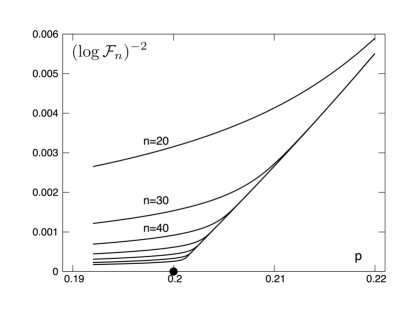
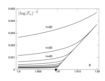
Figure 2: According to (12), the plot $(\log{\cal F}_{n})^{-2}$ versus $\Delta$ (here $\Delta$ is proportional to $p$) should vanish linearly at the transition point $p_{c}$. The two curves show this plot for the two distributions (11) and (17) in the case $\alpha=6$. (From (6,7) the exact values of $p_{c}$ shown by small black circles can be determined: $p_{c}=.2$ and $p_{c}=1.90956...$). As $n$ increases, the linearity of the plot looks better and bettter.

   

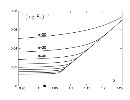
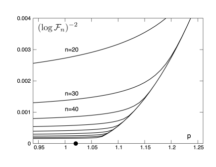
Figure 3: In contrast to the two examples of Figure 2, it is the plot of $(-\log{\cal F}_{n})^{-1}$ which should be linear (see (15)) for the distribution (17) when $\alpha=3$. This behavior is clearly seen in this case, in the vicinity of the exact critical point $p_{c}\simeq 1.02031...$. On the other hand, if one plots $(\log{\cal F}_{n})^{-2}$ as in Figure 2, the shape does not look linear indicating that (12) is no longer valid.

Remark: the above critical behaviors (12,15) as well as the conjecture (9) do remain valid [7] when, for any integer $m\geq 3$, the recursion (2) is replaced by

$$X_{n}=\max\left[X_{n-1}^{(1)}+X_{n-1}^{(2)}\cdots+X_{n-1}^{(m)}-1,0\right]$$ (18)

provided that (7,9,13,14) are modified to become

$$H_{0}(m)-m(m-1)H^{\prime}_{0}(m)=0\ \ \ \ \ ;\ \ \ \ 1-H_{n}(0)\simeq{4\over(m-1)^{2}\ n^{2}}$$

and

$$H_{0}^{\prime\prime\prime}(m)<\infty\ \ \ \ \ ;\ \ \ \ P(X_{0}=k)\simeq{{\rm Constant}\over m^{k}\ k^{\alpha}}\ \ .$$

1.2 Outline of the present paper

One of the goals of the present paper is to analyze the case (14) from the perspective of the continuous equation (1). We will see in Section 3 that, along the critical manifold ($\Delta=0$), the distribution $P(X_{n})$ takes a scaling form which depends on $\alpha$ for $2<\alpha<4$ and that this scaling form is described by particular solutions of (1). We will also see in Section 4 how the $\alpha$-dependent critical behavior (15) emerges from the linearization of (1) in the vicinity of the critical manifold. In section 5 we will discuss the shape of the tree connecting, at criticality and in the scaling regime, some non zero value $X_{n}$ to the initial values $X_{0}$. But we will start in section 2 by recalling a few known facts about the relation between the discrete problem (2) and the continuous equation (1).

2 The relation between the continuous equation (1) and the discrete problem (2,3)

Based on the analysis of numerical studies of the recursion (2) in [12] it was noticed that, after a transient time and in the neighborhood of the critical manifold ($\Delta\ll 1$), the distribution $P(X_{n})$ evolves very slowly and that the data were consistent, for $k\geq 1$, with a scaling form

$$P(X_{n}=k)\equiv Q_{n}(k)\simeq{u^{2}\over 2^{k}}\ f\left(u\,k,u\,n\right)$$ (19)

where $u$ is a small parameter. In the scaling regime, defining $x$ and $t$ by

$$k={x\over u}\ \ \ \ \ ;\ \ \ \ n={t\over u}$$ (20)

and inserting these forms into the recursion (4) for $k\geq 1$ one obtains (1) by keeping the leading order in $u$.

For distributions of the form (19) one can also see (by keeping the leading order in $u$) that the critical manifold (6,7) becomes

$$\int_{0}^{\infty}xf(x,0)dx=1$$ (21)

and that (9,6,16)

$$1-P(X_{n}=0)\simeq u^{2}f(0,{u\,n})\ \ \ \ \ ;\ \ \ \ \ \Delta=\int_{0}^{\infty}xf(x,0)dx-1$$ (22)

and

$${\langle X_{n}\rangle\over 2^{n}}\simeq 2^{1-{t\over u}}\ u^{2}\ f(0,t)\ \ .$$ (23)

(One can check that (21) remains invariant under the evolution (1).)

It was shown in [12] that one particular solution of (1) is

$$f(x,t)={4\kappa^{2}\over\sin[\kappa(t+t_{0})]^{2}}\ \exp\left[-{2\kappa\,x\over\tan[\kappa(t+t_{0})]}\right]$$ (24)

where $\kappa$ and $t_{0}$ can be arbitrary ($\kappa$ could be real or purely imaginary). For this distribution one has

$$\Delta={1\over\cos(\kappa\,t_{0})^{2}}-1$$ (25)

so that $\Delta>0$ corresponds to $\kappa$ real (with $0<\kappa\,t_{0}<2\pi$), and $\Delta<0$ corresponds to $\kappa$ purely imaginary. Along the critical case $\Delta=0$ (given by $\kappa=0$)

$$f(x,t)={4\over(t+t_{0})^{2}}\ \exp\left[-{2x\over t+t_{0}}\right]$$ (26)

and it is easy to see (20,22) that (9) is satisfied in the limit $n\to\infty$.

For $\Delta>0$ (i.e. for $\kappa$ real), it is clear that the solution (24) diverges as $t\to t_{c}$ where

$$t_{c}\equiv{\pi\over\kappa}-t_{0}$$ (27)

(because $\tan(\kappa(t+t_{0}))\to 0^{-}$).

When $t$ approaches this limit, the scaling form (19) ceases to be valid (i.e. the system exits the scaling regime and $P(X_{n})$ is no longer given by (19)). This can be seen in particular in the expression (22) where the divergence of $f(x,t)$ would make $P(X_{n}=0)$ become negative which is not possible. For $n\geq{t_{c}\over u}$, the probability $P(X_{n}=0)$ becomes small, so that one can forget the events where $X_{n}=0$ and one can replace the recursion (2) by simply $X_{n+1}=X_{n}^{(1)}+X_{n}^{(2)}-1$. This leads to the following expression of ${\cal F}_{\infty}$ defined by (3) when $t\to t_{c}$ (see (23))

$${\cal F}_{\infty}\sim{\cal F}_{n={t_{c}\over u}}\sim 2^{-{t_{c}\over u}}$$ (28)

(one way to justify (28) is to say that, for $u$ small, the scaling (23) form remains valid as long as $t_{c}-t\geq u$). As the limit $\Delta\to 0^{+}$ corresponds to the limit $\kappa\to 0$ (see (25)) which gives $\Delta\simeq{\kappa^{2}t_{0}^{2}\over 2}$ one gets from (28, 27)

$${\cal F}_{\infty}\sim 2^{-{\pi\over u\,\kappa}}\sim 2^{-{\pi\,t_{0}\over\sqrt{2}u}\,{1\over\sqrt{\Delta}}}$$ (29)

in agreement with (12).

Remark: any initial condition $f(x,0)$ consisting of a single exponential can be written as (24) by adjusting the parameters $\kappa$ and $t_{0}$. For more general initial conditions $f(x,0)$, one expects that

$$\begin{array}[]{ccccc}f(x,t)\to&\ 0&&{\rm as}\ \ \ t\to\ \infty&{\rm for}\ \ \ \Delta\leq 0\\ f(x,t)\to&\ \infty&&{\rm as}\ \ \ t\to\ t_{c}(\Delta)&{\rm for}\ \ \ \Delta>0\end{array}$$

depending on the sign of $\Delta$ defined in (22). Then, as in (28,29), knowing how $t_{c}(\Delta)$ diverges as $\Delta\to 0$ allows one to predict the critical behavior of ${\cal F}_{\infty}$.

As for recursion (2) we will see that (29) is expected to hold only when condition (13) is fulfilled which, in the context of (1), means that

$$\int_{0}^{\infty}x^{3}\,f(x,0)dx<\infty\ \ .$$ (30)

Remark: we will see in Section 4 that both the critical behaviors (12) and (15) can also be understood by linearizing (1) in the neighborhood of the scaling function (26) as well as of the other scaling functions discussed in Section 3.2.

Remark: for distributions of the type (14), when $\alpha<2$ one has $\Delta=\infty$ (see (6)) so that taking the limit $\Delta\to 0^{+}$ is meaningless. One expects however [20] in this case that for distributions of the form (17)

$${\cal F}_{\infty}\sim\exp\left[-\ p^{-{1\over 2-\alpha}+o(1)}\right] \ \ \ \ \ \ {\rm as}\ \ p\to 0\ \ .$$ (31)

From the view point of (1) it is easy to check that, if $f(x,t)$ is the solution of (1) for the initial condition $f(x,0)=x^{-\alpha}$, then $f^{*}(x,t)=p^{2\over 2-\alpha}f(x\,p^{1\over 2-\alpha},t\,p^{1\over 2-\alpha})$ is the solution of (1) for the inititial condition $f^{*}(x,0)=p\,x^{-\alpha}$. Therefore if $f(x,t)$ blows up at some critical time $t_{c}$, then $f^{*}(x,t)$ blows up at time $t_{c}^{*}=p^{-{1\over 2-\alpha}}\,t_{c}$ and repeating the reasoning going from (28) to (29) leads to (31).

Remark: motivated by the discrete problem (2), Hu, Mallein and Pain proposed in [19] a continuous space-time continuous version of the model whose evolution differs from (1)

$${{df(x,t)\over dt}=-f(x,t)+{df(x,t)\over dx}+{1\over 2}\int_{0}^{x}f(x-y,t)f(y,t)dy}\ \ .$$ (32)

For this problem too they were able to find a family of exact solutions consisting of a single exponential allowing them to prove the critical behavior (12).

3 Families of exact solutions of (1)

In [12] the main predictions (9,12) were based on the exact solution (24) of (1). In this section we will exhibit several other families of solutions of (1). Our interest is limited to solutions of (1) with non negative initial conditions ($f(x,0)\geq 0$) because $P(X_{0}=k)$ is a probability distribution (19). Intuitively it is clear that, since (1) was obtained through the scaling (19), $f(x,t)$ should remain non-negative at $t>0$. A proof that evolving (1) with a non-negative initial condition $f(x,0)$ leads to a non-negative solution $f(x,t)$ is given in A.

3.1 The fixed points of (1)

As shown in B, one can find a fixed point solution (i.e. a time independent solution) $f(x)$ of (1) for any choice of $f(0)$. All these solutions can be expressed in terms of a Bessel function whose sign varies along the positive real axis. Therefore there is no way that such fixed point solutions can be reached or approached if one evolves (1) starting with a non-negative initial condition $f(x,0)$. So we can forget these fixed point solutions.

3.2 The scaling functions

An important family of solutions of (1) which will be central in our understanding of (15) are scaling solutions of the form

$$f(x,t)={1\over(t+t_{0})^{2}}F\left({x\over t+t_{0}}\right)\ \ .$$ (33)

They generalize (26). Inserting (33) into (1) one gets immediately that the scaling function $F$ should satisfy

$$xF^{\prime}+2F+F^{\prime}+{1\over 2}\int_{0}^{x}F(y)F(x-y)\ dy=0\ \ .$$ (34)

For an arbitrary value $F_{0}$ of $F(0)$ one can solve (34) in powers of $x$ or in powers of $F_{0}$:

$$F(x) = F_{0}-2F_{0}\ x+\left(3F_{0}-{F_{0}^{2}\over 4}\right)x^{2}+\left(-4F_{0}+{2F_{0}^{2}\over 3}\right)x^{3}+O(x^{4})$$ (35)

$$= {F_{0}\over(1+x)^{2}}+F_{0}^{2}\left({x\over 2(1+x)^{2}(2+x)}-{\log(1+x)\over(2+x)^{2}}\right)+O(F_{0}^{3})\ \ .$$

Apart from the special case $F_{0}=4$ for which $F(x)=4e^{-2x}$ (see (26)) it is not clear whether these series in powers of $x$ or in powers of $F_{0}$ converge, nor can one tell from these expansions for which values of $F_{0}$, the scaling function $F$ remains non-negative. One can however integrate numerically (34) as in Figure 4. Except for $F_{0}=4$, one can observe a power law decay of $F(x)$ and that for $F_{0}>4$ the solution becomes negative.  
 

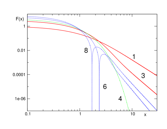
Figure 4: The solution $F(x)$ of (34) (or rather its absolute value $|F(x)|$ in the cases $F(0)=6$ or $8$) for several choices ($F(0)=1,3,4,6,8$) of $F(0)$. Except for $F(0)=4$ the large $x$ decay is a power law $F(x)\sim x^{-\alpha}$. We will see (46) that $\alpha=1+\sqrt{1+2F(0)}$ . As here the figure shows a log-log plot of $|F(x)|$, the zeroes of $F(x)$ appear as singularities (where $\ln|F(x)|\to-\infty$) in the cases $F(0)=6$ or $8$.

In order to go further, it is easier to work with Laplace transforms. The Laplace transform $\widetilde{f}$ of $f$

$$\widetilde{f}(p,t)=\int_{0}^{\infty}f(x,t)\ e^{-px}dx$$ (36)

evolves (see (1)) according to

$${d\widetilde{f}(p,t)\over dt}=-f(0,t)+p\widetilde{f}(p,t)+{1\over 2}\widetilde{f}(p,t)^{2}\ \ .$$ (37)

For scaling solutions of the form (33) the Laplace transform $\widetilde{f}$ of $f$ takes also a scaling form

$$\widetilde{f}(p,t)={1\over t+t_{0}}\widetilde{F}(p(t+t_{0}))$$ (38)

where $\widetilde{F}(q)$ satisfies

$$\widetilde{F}+q\widetilde{F}+{1\over 2}\widetilde{F}^{2}-F(0)-q\widetilde{F}^{\prime}=0\ \ .$$ (39)

This is a non-linear equation! It turns out that it can be solved in terms of Bessel functions: if one looks for a solution of the form

$$\widetilde{F}(q)=-1-q-q\ {y^{\prime}({q\over 2})\over y({q\over 2})}$$ (40)

one gets from (39) that $y(q)$ should satisfy

$$q^{2}y^{\prime\prime}+qy^{\prime}-\left(q^{2}+\beta^{2}\right)y=0\ \ \ \ \ {\rm where}\ \ \beta^{2}={1\over 4}+{F(0)\over 2}\ \ .$$ (41)

As $y$ is solution of a second order equation, it depends a priori on two arbitrary constants. For example for large $q$ it depends on the two constants $B$ and $B^{\prime}$:

$$y= B\ {e^{-q}\over\sqrt{q}}\left(1+{4\beta^{2}-1\over 8\ q}+{(4\beta^{2}-1)(4\beta^{2}-9)\over 128\ q^{2}}+\cdots\right)$$ (42)

$$+ B^{\prime}\ {e^{q}\over\sqrt{q}}\left(1-{4\beta^{2}-1\over 8\ q}+{(4\beta^{2}-1)(4\beta^{2}-9)\over 128\ q^{2}}\ \ .+\cdots\right)\ \ .$$

If $B^{\prime}\neq 0$ then $\widetilde{F}(q)\simeq-2q$ for large $q$ which cannot be as $\widetilde{F}(q)$ is the Laplace transform of a non-negative function. Therefore $B^{\prime}=0$. Moreover only the logarithmic derivative of $y$ is needed (see (40)) so that the choice of the constant $B$ does not matter. Therefore one can choose for $y$ the modified Bessel function $K_{\beta}$:

$$y=K_{\beta}(q)\equiv\int_{0}^{\infty}dt\,\cosh(\beta t)\ \exp[-q\cosh(t)]\ \ .$$ (43)

From (42) (with $B^{\prime}=0$) one gets for large $q$

$$\widetilde{F}(q)={4\beta^{2}-1\over 2q}-{4\beta^{2}-1\over q^{2}}-{(4\beta^{2}-1)(4\beta^{2}-25)\over 8q^{3}}+\cdots$$

This coincides, as it should, with the large $q$ expansion which can be obtained directly from (39)

$$\widetilde{F}(q)={F(0)\over q}-{2F(0)\over q^{2}}+{F(0)(12-F(0))\over 2q^{3}}+\cdots$$

when $F(0)$ and $\beta$ are related as in (41).  
 
For small $q$, one can also show from (43) that

$$y(q)\simeq \ 2^{\beta-1}\ q^{-\beta}\left(\Gamma(\beta)-q^{2}{\Gamma(\beta-1)\over 4}+q^{4}{\Gamma(\beta-2)\over 32}+\cdots\right)$$

$$+2^{-\beta-1}\ q^{\beta}\left(\Gamma(-\beta)-q^{2}{\Gamma(-\beta-1)\over 4}+q^{4}{\Gamma(-\beta-2)\over 32}+\cdots\right)$$

which gives using (40)

$$\widetilde{F}(q)= \left((2\beta-1)-q+{q^{2}\over 4(\beta-1)}-{q^{4}\over 64(\beta-1)^{2}(\beta-2)}+\cdots\right)$$

$$+\ c(\beta)\,q^{2\beta}\left(1+{q^{2}\over 8(\beta-1)}+\cdots\right)\ +\ c(\beta)^{2}\,q^{4\beta}\left({1\over 4\beta}+\cdots\right)+\cdots$$

where

$$c(\beta)=2^{2-4\beta}{\Gamma(1-\beta)\over\Gamma(\beta)}\ \ .$$ (45)

The non-analytic term in the small $q$ expansion determines the large $x$ decay of the scaling function $F(x)$

$$F(x)\simeq{c(\beta)\over\Gamma(-2\beta)\ x^{1+2\beta}}={2^{4-2\alpha}\Gamma({3-\alpha\over 2})\over\Gamma(1-\alpha)\ \Gamma({\alpha-1\over 2})}{1\over x^{\alpha}}\ \ \ \ \ {\rm where}\ \ \alpha=1+2\beta=1+\sqrt{1+2F(0)}\ \ \$$ (46)

(see (41)). So varying $F(0)$, i.e. varying $\beta$, changes the power-law decay of the scaling function $F$.  
 
Remark: in (3.2) one should reorder the terms in the small $q$ expansion depending on the value of $\beta$. For example for ${1\over 2}<\beta<1$

$$\widetilde{F}(q)=(2\beta-1)-q+c(\beta)\,q^{2\beta}+O(q^{2})$$

whereas for $1<\beta<{3\over 2}$

$$\widetilde{F}(q)=(2\beta-1)-q+{q^{2}\over 4(\beta-1)}+\ c(\beta)\ q^{2\beta}+o(q^{3})\ \ .$$

Remark: we did not treat the cases where $\beta$ is an integer or half an integer. They could be analyzed as limiting cases of (3.2). For half integer values of $\beta$ there are only a finite number of terms in the sums (42) and $\widetilde{F}$ is a rational function. For example

$$\widetilde{F}(q) ={4\over q+2}\ \ \ \ \ {\rm for}\ \ \beta={3\over 2}$$

$$\widetilde{F}(q) ={12(q+4)\over q^{2}+6q+12}\ \ \ \ \ {\rm for}\ \ \beta={5\over 2}$$ (47)

$$\widetilde{F}(q) ={24(q^{2}+10q+30)\over q^{3}+12q^{2}+60q+120}\ \ \ \ \ {\rm for}\ \ \beta={7\over 2}\ \ .$$

Except for the case $\beta={3\over 2}$ which corresponds to the scaling function (26), these solutions do not remain non-negative along the whole positive real axis. For example for $\beta={5\over 2}$ one gets

$$F(x)=12e^{-3x}\cos(\sqrt{3}x)+4\sqrt{3}e^{-3x}\sin(\sqrt{3}x)$$ (48)

which obviously does not remain positive along the whole real axis. So as for the fixed points of (1) one can forget these solutions.

The particular solutions (47) correspond to the following expressions of $y(q)$

$$y(q) ={q+1\over q^{3\over 2}}\ e^{-q}\ \ \ \ \ {\rm for}\ \ \beta={3\over 2}$$

$$={q^{2}+3q+3\over q^{5\over 2}}\ e^{-q}\ \ \ \ \ {\rm for}\ \ \beta={5\over 2}$$

$$={q^{3}+6q^{2}+15q+15\over q^{7\over 2}}\ e^{-q}\ \ \ \ \ {\rm for}\ \ \beta={7\over 2}\ \ .$$

Remark: we believe, but did not succeed to prove from (40), that $\widetilde{F}(q)$ is the Laplace transform of a non-negative function $F(x)$ when $2<\alpha\leq 4$. One can however see that the tail (46) is negative for $0\leq\alpha<2$, $4<\alpha<6$, $8<\alpha<10$, etc . Moreover for $\alpha>4$, that is for $\beta>3/2$, the expansion (3.2) gives $\widetilde{F}(q)=2\beta-1-q+{q^{2}\over 4(\beta-1)}+o(q^{3})$ which implies that $\int_{0}^{\infty}x^{3}F(x)dx=0$. Therefore the scaling function cannot be non-negative on the entire positive real axis for $\alpha>4$. (In Figure 4 it was already clear that the scaling function $F(x)$ has at least one zero for $\alpha>4$.)  
 
Remark: it is easy to see that for $2<\alpha\leq 4$ (remember (46) that $\alpha=1+2\beta=1+\sqrt{1+2F(0)}$), the large $t$ decay of the scaling solutions (33) is

$$f(0,t)\simeq{F(0)\over t^{2}}={\alpha(\alpha-2)\over 2\,t^{2}}$$

If one comes back (see (19)) to $P(X_{n})$ this means that

$$1-P(X_{n}=0)=\sum_{k\geq 1}P(X_{n}=k)\simeq u^{2}f(0,t)\simeq{\alpha(\alpha-2)\over 2\,n^{2}}$$ (49)

to be compared with (9) when condition (13) is fulfilled.

Figure 5 shows the product $n^{2}\Big{(}1-P(X_{n}=0)\Big{)}$ versus $1/n$ (with $P(X_{n}=k)$ obtained by iterating (2)) for the three initial conditions already considered in Figures 2 and 3. For the two delta-peak distribution and for the distribution (17) with $\alpha=6$ the data confirm (9), indicating that the large $n$ asymptotics of $P(X_{n})$ is described by (26). When condition (13) is not satisfied, here in the case of (17) with $\alpha=3$, the data are consistent with (49) suggesting that the asymptotics follow the $\alpha$-dependent scaling function $F(x)$.

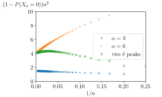
Figure 5: For the two delta peak distribution (11) (at criticality i.e. for $p={1\over 5}$) as well for the distribution (17) when $\alpha=6$ (at criticality i.e. for $p=1.90956...$), which both satisfy condition (13), the large $n$ asymptotics agrees with the prediction (9) that $n^{2}(1-P(X_{n}=0))\to 4$. On the other hand for (17) with $\alpha=3$ (at criticality i.e. for $p=1.02031...$) which does not satisfy condition (13), one observes the asymptotics (49), i.e. $n^{2}(1-P(X_{n}=0))\to\alpha(\alpha-2)/2$.

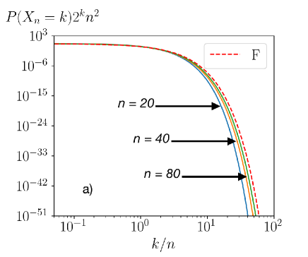
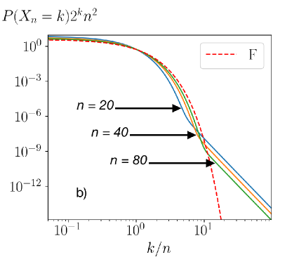
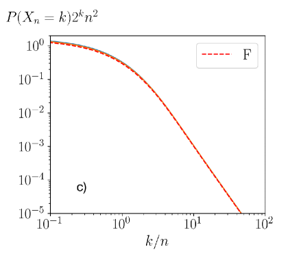
Figure 6: We compare the scaling functions (33) solutions of (34) (dashed lines) with the solutions of (4) for the same three cases as in Figure 5 at times $n=20$, $40$ and $80$. As $n$ increases the convergence to $F$, the expected scaling function (26), is better and better for the two delta peak distribution (figure a) and for the distribution (17) with $\alpha=6$ (figure b). For the distribution (17) with $\alpha=3$ the convergence is even faster (figure c) but the scaling function, solution of (34), is different. It is the one with $F(0)={3\over 2}$ (see (46)).

Figure 6 compares the scaling functions solutions (33) solution of (34) with the the distributions $P(X_{n})$ obtained by a numerical iteration of (4) with an initial condition which is either a two delta peaks (11) with $p=1/5$ or (17) for $\alpha=6$ and $\alpha=3$. In all cases the expected convergence to the scaling function is observed.

3.3 Sums of exponentials

One can build another family of exact solutions of (1) which generalizes (24): if the initial condition is the sum of exponentials, then the solution at all times remains a sum of exponentials

$$f(x,t)=\sum_{i}a_{i}(t)e^{x\,b_{i}(t)}$$ (50)

with the parameters $a_{i}(t)$ and $b_{i}(t)$ evolving according to

$$\dot{a_{i}} =a_{i}\ b_{i}+a_{i}\sum_{j\neq i}{a_{j}\over b_{i}-b_{j}}$$

$$\dot{b_{i}} ={a_{i}\over 2}$$ (51)

(The scaling function (33,48) was an example of such a solution in the case of two exponentials).

It is easy to check that

$$\sum_{i}a_{i}-b_{i}^{2}={\rm Constant}$$ (52)

is left invariant by the evolution (51). One can also verify that initial conditions on the critical manifold (21), i.e. such that

$$\sum_{i}{a_{i}\over b_{i}^{2}}=1$$ (53)

remain on the critical manifold. Apart from these two invariants (52,53), it is in general difficult to integrate the evolution (51).

Along the critical manifold (53) however, one can find the general solution of (1) when it consists of a sum of two exponentials. It is of the form

$$f(x,t)=2\ {db_{1}(t)\over dt}\ e^{x\,b_{1}(t)}+2\ {db_{2}(t)\over dt}\ e^{x\,b_{2}(t)}$$ (54)

where $b_{1}(t)$ and $b_{2}(t)$ are given by

$$b_{1,2}(t)=-{4K\over K(t+t_{1})\pm\sqrt{K^{2}(t+t_{1})^{2}-4K(t+t_{1})\tanh(K(t+t_{0}))+4}}$$ (55)

where the free parameters $t_{0},t_{1}$ and $K$ could be determined from the initial condition  $a_{1}(0),a_{2}(0),b_{1}(0),b_{2}(0)$. (Here one needs to satisfy the condition (52) to be on the critical manifold together with $b_{1}(0)<0$ and $b_{2}(0)<0$, and this is why one is left in (55) with only 3 parameters.)

For real $K,t_{0}$ and $t_{1}$ this gives in the long time limit

$$b_{1}\simeq-{2\over t}\ \ \ ;\ \ \ a_{1}\simeq{4\over t^{2}}\ \ \ \ \ \ \ {\rm and}\ \ \ \ \ \ \ b_{2}\to-2K\ \ ;\ \ a_{2}\simeq 16K^{2}e^{-2K(t+t_{0})}\ \ .$$

This shows that $a_{2}$ decays very fast, so that a single exponential dominates and the solution becomes given by (26).

In fact, on the critical manifold (21), for any non negative intial condition consisting of a finite number of decreasing exponentials, one expects that in the long time limit, all the amplitudes $a_{i}$ decay exponentially except one and that, asymptotically, the solution is given by (26).  
 
Remark: by taking $t_{1}=0$, $t_{0}=i{\pi\over 2K}+{8K^{2}\over p}$ and then the limit $K\to 0$ one finds

$$b_{1,2}={3\,p\,t^{2}\pm\sqrt{288\,pt-3\,p^{2}\,t^{4}}\over 24-p\,t^{3}}$$

which corresponds to the initial condition $f(x,0)=p\,x$. One can notice that this solution blows up at a time $t_{c}=(24/p)^{1\over 3}$ as expected in (31) in the case $\alpha=-1$.  
 
Remark: the single exponential (24) is also a particular case of (55) as it corresponds to the limit $t_{1}\to\infty$.  
 
Remark: in [19], it was also noticed that finite sums of exponentials with time-dependent parameters solve the equation (32). Equations similar to (51) but simpler were also discussed [22] in the context of integrable systems and random polynomials.  
 

4 Expanding around the scaling functions

We have obtained in Section 3.2 a one parameter family of solutions (33) which all lie on the critical manifold. In this section we discuss the evolution of small perturbations around these scaling functions. To do so we consider solutions of (1) of the form

$$f(x,t)={1\over(t+t_{0})^{2}}F\left({x\over t+t_{0}}\right)+\epsilon\ g(x,t)$$

or equivalently

$$\widetilde{f}(p,t)={1\over t+t_{0}}\widetilde{F}\Big{(}p(t+t_{0})\Big{)}+\epsilon\ \widetilde{g}(p,t)\ \ .$$ (56)

with $\widetilde{F}$ given by (40). Then at order $\epsilon$, $\widetilde{g}$ evolves according to

$${d\widetilde{g}(p,t)\over dt}=-g(0,t)+p\,\widetilde{g}(p,t)+{1\over t+t_{0}}\widetilde{F}\big{(}p(t+t_{0})\big{)}\ \widetilde{g}(p,t)\ \ .$$ (57)

Although this equation is linear, it is non-local in the $q$ variable, because of the presence of $g(0,t)$, and we did not succeed in finding an explicit solution for an arbitrary initial condition $\widetilde{g}(p,0)$.

One can however obtain “eigenfunctions” corresponding to this linear evolution: if one chooses $g(x,t)$ or $\widetilde{g}(p,t)$ of the form

$$g(x,t)=(t+t_{0})^{\gamma-2}\ G_{\gamma}\left({x\over t+t_{0}}\right)\ \ \ \ \ \Longleftrightarrow\ \ \ \ \ \widetilde{g}(p,t)={(t+t_{0})^{\gamma-1}}\ \widetilde{G}_{\gamma}\Big{(}p(t+t_{0})\Big{)}$$ (58)

where $\gamma$ plays the role of an eigenvalue, one gets from (57) that $\widetilde{G}_{\gamma}$ should satisfy

$$q\widetilde{G}_{\gamma}(q)+\widetilde{F}(q)\widetilde{G}_{\gamma}(q)-q\widetilde{G}_{\gamma}^{\prime}(q)-(\gamma-1)\widetilde{G}_{\gamma}(q)=G_{\gamma}(0)\ \ .$$ (59)

Replacing $\widetilde{F}$ by its expression (40) one finds for $\widetilde{G}_{\gamma}$

$$\widetilde{G}_{\gamma}(q)=G_{\gamma}(0)\ q^{-\gamma}\,\left[y\left({q\over 2}\right)\right]^{-2}\int_{q}^{\infty}q_{1}^{\gamma-1}\left[y\left({q_{1}\over 2}\right)\right]^{2}dq_{1}$$ (60)

(one has to choose the solution of (59) which decays in the limit $q\to\infty$ and this fixes the arbitrary constant in the solution of the linear differential equation (59)). For small $q$ one gets formally from (60) or directly by solving (59)

$$\widetilde{G}_{\gamma}(q)={G_{\gamma}(0)\over 2\beta-\gamma}-{G_{\gamma}(0)\ q^{2}\over 4(2\beta-\gamma)(2\beta-\gamma-2)(\beta-1)}+\cdots$$

$$+c(\beta)\,q^{2\beta}\left({G_{\gamma}(0)\over(\gamma+2)(2\beta-\gamma)}+\cdots\right)+$$ (61)

$$+d(\beta,\gamma)\ q^{2\beta-\gamma}\left(G_{\gamma}(0)+\cdots\right)\ +\cdots$$

where $c(\beta)$ is given by (45) and $d(\beta,\gamma)$ takes different forms depending on the values of $\beta$ and $\gamma$. For example for $\gamma-2\beta>0$, one has

$$d(\beta,\gamma)=4\int_{0}^{\infty}q_{1}^{\gamma-1}\left[y\left({q_{1}\over 2}\right)\right]^{2}dq_{1}$$

whereas for $-1<\gamma-2\beta<0$, one has

$$d(\beta,\gamma)=4\int_{0}^{\infty}q_{1}^{\gamma-1}\left(\left[y\left({q_{1}\over 2}\right)\right]^{2}-2^{2\beta-2}\ \Gamma(\beta)^{2}\ q_{1}^{-2\beta}\right)dq_{1}\ \ .$$

(This is reminiscent of the various integral expressions of the $\Gamma$ function.)

As in (3.2) one needs to reorder the terms in (61) by increasing powers of $q$ in the various sectors of $\gamma-2\beta$ .  
 
Remark: for general $\beta$ and $\gamma$ we could not find expressions of $\widetilde{G}_{\gamma}(q)$ simpler than (60). However, in the case $\gamma=-1$, one can easily check that

$$\widetilde{G}_{-1}(q)={G_{-1}(0)\over 2F(0)}\Big{(}\widetilde{F}(q)-q\widetilde{F}^{\prime}(q)\Big{)}$$ (62)

and that in the case $\gamma=0$

$$\widetilde{G}_{0}(q)=G_{0}(0)\ {\partial\widetilde{F}(q)\over\partial F(0)}\ \ .$$

Also for particular values of $\beta$ and $\gamma$ the eigenfunction $\widetilde{G}_{\gamma}(q)$ is rational and one can get some closed expressions. For example for $\beta$ half-integer and $\gamma=2\beta-1$

$$\widetilde{G}_{2}(q) =G_{2}(0)\ {q+4\over(q+2)^{2}}\ \ \ \ \ {\rm for}\ \ \beta={3\over 2}$$

$$\widetilde{G}_{4}(q) =G_{4}(0)\ {q^{3}+14q^{2}+74q+144\over(q^{2}+6q+12)^{2}}\ \ \ \ \ {\rm for}\ \ \beta={5\over 2}$$

and so on.

A priori, to understand the neighborhood of the scaling solution (56), one could try to decompose the initial perturbation $\widetilde{g}(p,0)$ on the eigenfunctions (60). We did not succeed in doing this decomposition. One can however analyze the long time behavior of perturbations as $\gamma$ varies.

• For $\gamma<0$, we see in (56,58) that the perturbation becomes much smaller than the dominant term in (56). In the particular case $\gamma=-1$ (see (62)) the perturbation is nothing but a shift of order $\epsilon$ of the time $t_{0}$. So asymptotically the perturbation disappears.
  

• For $0<\gamma<2\beta-1$ the perturbation is relevant, in the sense that the perturbation in (56) grows faster than the dominant term. Still as long as $\gamma<2\beta-1$ the perturbation leaves the solution on the critical manifold (21) (because there is no linear term in $q$ in (61) so that (21) remains unchanged). It is clear from (61) that the large $x$ decay of the perturbation $G_{\gamma}(x)\sim x^{\gamma-2\beta-1}$ is slower that the decay $F(x)\sim x^{-2\beta-1}$ of the dominant term in (56). Therefore one expects to observe in the long time limit another scaling function $F$, the one corresponding to $2\beta$ being replaced by $2\beta-\gamma$.
  

• For $\gamma=2\beta-1$, the perturbation moves the initial condition away from the critical manifold and

  $$\int_{0}^{\infty}x\,f(x,0)dx=1+O(\epsilon)\ \ .$$

  In this case the perturbation remains small compared to the leading term in (56) as long as $\epsilon\ t^{\gamma}<1$ . Therefore one expects a critical time $t_{c}$ to scale with the distance $\epsilon$ to the critical manifold to scale like

  $$t_{c}\sim\epsilon^{-{1\over\gamma}}=\epsilon^{-{1\over 2\beta-1}}=\epsilon^{-{1\over\alpha-2}}\ \ .$$

  By repeating the same argument (28) which led to (29) one can then recover (15).
  

• For $\gamma>2\beta-1$, one has $f(x,0)\sim g(x,0)\sim x^{\gamma-2\beta-1}$ for large $x$ (due to the term $q^{2\beta-\gamma}$ in (61)) and one expects a singularity of the form (31), i.e. ${\cal F}_{\infty}\sim\exp[-\epsilon^{-{1\over\gamma-2\beta+1}+o(1)}]$.

5 The critical trees

To each realization of the process (2) leading to a non-zero value of $X_{n}$, one can associate a random tree, representing how this value of $X_{n}$ is obtained. This tree connects this value $X_{n}$ to all the non-zero values of $X_{k}$ which contribute to $X_{n}$. It can be constructed according to the following recursive rule for $1\leq m\leq n$: one starts at the bottom of the tree with the value $X_{n}$. Then if $X_{m}$ is a non-zero value on this tree at level $m$,

• either there is no branching between level $m$ and $m-1$ and $X_{m-1}=X_{m}+1$ with a probability

  $${\rm Pro}(X_{m-1}|X_{m})\ =\ {2\,Q_{m-1}(X_{m}\,+\ 1)\ Q_{m-1}(0)\over Q_{m}(X_{m})}\ \delta(X_{m-1},X_{m}+1)\ \ .$$

• or there is a branching event between level $m$ and $m-1$ with probability $1-2\,Q_{m-1}(X_{m}+1)\,Q_{m-1}(0)/Q_{m}(X_{m})$ leading to two non-zero random values $X_{m-1}^{(1)}$ and $X_{m-1}^{(2)}$ at level $m-1$ with a probability

  $${\rm Pro}(X_{m-1}^{(1)},X_{m-1}^{(2)}|X_{m})={Q_{m-1}(X_{m-1}^{(1)})\ Q_{m-1}(X_{m-1}^{(2)})\over{Q_{m}(X_{m})-2\,Q_{m-1}(X_{m}+1)Q\,_{m-1}(0)}}\ \delta(X_{m-1}^{(1)}+X_{m-1}^{(2)}\ ,\ X_{m}+1)\ \ .$$ (63)

It follows immediately from this construction that the probability ${\cal P}_{m^{\prime},m}(X_{m})$ that there is no branching up to the level $m^{\prime}$, if one starts at a value $X_{m}$ at the $m$-th level of the tree, is

$${\cal P}_{m^{\prime},m}(X_{m})=2^{m-m^{\prime}}\ {Q_{m^{\prime}}(X_{m}+m-m^{\prime})\over Q_{m}(X_{m})}\prod_{\mu=m^{\prime}}^{m-1}Q_{\mu}(0)\ \ .$$ (64)

Using the scaling form (19) which relates the discrete problem (2) to the continuous time equation (1) and taking the limit $u\to 0$ one gets from (64) that, starting with a value $x$ at time $t$, the probability $\psi_{t^{\prime},t}(x)$ that there is no branching up to the time $t^{\prime}$ is

$${\psi}_{t^{\prime},t}(x)={f(x+t-t^{\prime},t^{\prime})\over f(x,t)}$$ (65)

(note that to leading order in $u$ the product in (64) does not contribute). Similarly, given that there is a branching at time $t$, the density probability $\Psi_{t}(x_{1},x_{2}|x)$ that a value $x$ splits into two value $x_{1}$ and $x_{2}$ is

$$\Psi_{t}(x_{1},x_{2}|x)={f(x_{1},t)\ f(x_{2},t)\over\int_{0}^{x}f(x^{\prime},t)f(x-x^{\prime},t)dx^{\prime}}\ \delta(x_{1}+x_{2}-x)\ \ .$$ (66)

The study of the above constructed tree on the critical manifold (7) was crucial [7] in the mathematical proofs of (12) and of (15). On the critical manifold (7), as one expects (see (19,33)) that in the large $n$ limit

$$2^{k}\ Q_{n}(k)\simeq{1\over n^{2}}\ F\left({k\over n}\right)$$

with $F$ solution of (34), these expressions become

$${\psi}_{t^{\prime},t}(x)=\left({t\over t^{\prime}}\right)^{2}\ {F({x+t-t^{\prime}\over t^{\prime}})\over F({x\over t})}$$ (67)

$$\Psi_{t}(x_{1},x_{2}|x)={F({x_{1}\over t})\ F({x_{2}\over t})\over\int_{0}^{x}F({x^{\prime}\over t})F({x-x^{\prime}\over t})dx^{\prime}}\ \delta(x_{1}+x_{2}-x)\ \ .$$ (68)

For initial distributions which decay fast enough (i.e. which satisfy (13) for the discrete time problem (2) or (30) for the continuous time problem (1)) one expects the scaling function $F$ to be given by $F(x)=4e^{-2x}$ so that the above expressions (67) and (68) become

$${\psi}_{t^{\prime},t}(x)=\left({t\over t^{\prime}}\right)^{2}\ e^{-{2(t-t^{\prime})(x+t)\over t\,t^{\prime}}}\ \ \ \ \ ;\ \ \ \ \Psi_{t}(x_{1},x_{2}|x)={1\over x}\ \ .$$ (69)

This leads to the same critical random trees as those obtained in [19] for the problem (32) which can be constructed in the present context as follows:

1. one starts with a single particle of mass $\mu_{t}=x$ at time $t$ at the bottom of the tree.

2. then going down in time the mass $\mu_{t}$ increases linearly $\mu_{t^{\prime}}=\mu_{t}+t-t^{\prime}$ until the first branching event at time $t^{\prime}$ is reached.

3. this branching event occurs at rate

   $${2\mu_{t^{\prime}}\over t^{\prime 2}}$$ (70)

   and the mass $\mu_{t^{\prime}}$ is split uniformly between two branches. The masses on these two branches continue to grow and to split independently up to time $0$, in the same way as the branch we started with at time $t$.

For initial distributions (on the critical manifold) which do not satisfy conditions (13) or (30), like (14, 17) for the discrete problem (2) or $f(x,0)\sim x^{-\alpha}$ for the continuous problem (1) for $2\leq\alpha<4$, the above expressions (67) and (68) remain valid if one chooses the scaling function $F$ solution (see section 3.2) which decays with the same power law $\alpha$ as the initial condition. In this case the critical random trees can also be constructed:

1. one starts with a single particle of mass $\mu_{t}=x$ at time $t$ at the bottom of the tree.

2. then going up in time the mass $\mu_{t}$ increases linearly $\mu_{t^{\prime}}=\mu_{t}+t-t^{\prime}$ until the first branching event at time $t^{\prime}$ is reached

3. this branching event occurs at rate

   $$-{2\over t^{\prime}}-\left({1\over t^{\prime}}+{\mu_{t^{\prime}}\over t^{\prime 2}}\right){F^{\prime}({\mu_{t^{\prime}}\over t^{\prime}})\over F({\mu_{t^{\prime}}\over t^{\prime}})}$$ (71)

   instead of (70). The way the mass is split remains given by (68) but is no longer uniform.

In Figure 7 we see that the expressions (64) obtained by the numerical iteration of (4) converge very well to the expected scaling form (67).

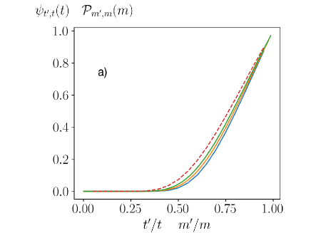
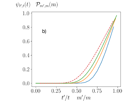
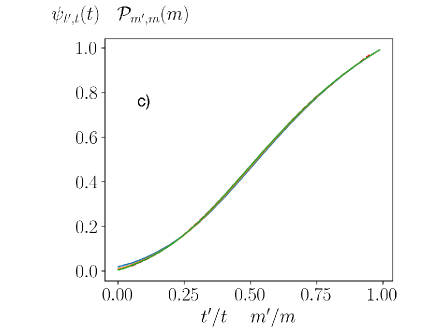
Figure 7: We compare the predictions (67) and (69) with the expressions (64) obtained by iterating numerically (4) for the probability of no branching up to time $m^{\prime}$ for two critical distributions which satisfy (13) and one which does not (the two delta peaks (11) with $p=p_{c}=.2$ (figure a) and the distribution (17) with $p=p_{c}=1.90956...$ for the case $\alpha=6$ (figure b) and with $p=p_{c}=1.02031..$ for the case $\alpha=3$ (figure c)). Here we choose as the starting point $X_{m}=m$. In the three cases, we draw the expression (64) for $m=20,40,80$. The expected convergence is very good if one chooses in each case the appropriate scaling function (69) for figures a and b and (67) using the scaling function $F$ with the right power law decay (here the one with $F(0)={3\over 2})$ in the case of figure c.

For the same three distributions as in Figure 7 one can also check in Figure 8 the convergence of the splitting probabilities (63) to their predicted scaling forms (66).

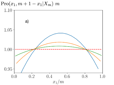
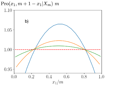
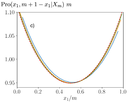
Figure 8: For the same three distributions as in Figure 7 and same sizes ($m=20,40,80$) we compare the spliting probabilities (63) to their scaling forms (68) which is drawn as a dashed line. We choose the starting point to be $X_{m}=m$. For the two delta peaks (figure a) and the case $\alpha=6$ (figure b) we observe the expected convergence of $m\ \mathrm{Pro}(x_{1},m+1-x_{1}|X_{m})$ to $1$. In the case $\alpha=3$ (figure c) one observes also a convergence but to (68) with the right choice of $F$, i.e here : $F(0)=3/2$.

Remark: all these random critical trees are scale invariant, in the sense that if all the masses and all the times are multiplied by a fixed factor: $t\to\lambda t$ and $x\to\lambda x$, they obey the same statistics as the above constructed trees.  
 
Remark: in the limit $F_{0}\to 0$, i.e. $\alpha\to 2$, the expression (35) gives $F(x)\simeq F_{0}/(1+x)^{2}+O(F_{0}^{2})$, so that all the branching rates (71) are of order $F_{0}$. This means that in this limit, the tree reduces to a single straight line: $\mu_{t}^{\prime}=\mu_{t}+t-t^{\prime}$. At the next order in $F_{0}$, one could see also trees with a single branching, and so on: each new order in the small $F_{0}$ expansion would add trees with an additional branching.

6 Conclusion

One of the main progress of the present work was to obtain exact expressions (34, 40) for a family of scaling functions solutions of (1). These scaling functions are indexed by a parameter $\alpha=1+2\beta=1+\sqrt{1+2F(0)}$ which controls their power law decay (46). They generalize the already known scaling function (26) which was at the origin of the conjecture (12). The analysis of the neighborhood of this family of scaling functions in section 4 confirmed all the other possible critical behaviors (15). We gave numerical evidence in Figure 4 that these scaling functions are positive on the whole positive real axis when $2<\alpha\leq 4$ and only in this range (see one of the remarks of section 3.2). We also saw in Figures 5 and 6 that, for the original problem (2), starting with initial conditions on the critical manifold the distribution properly rescaled converges asymptotically to one of these scaling functions: initial conditions whose large $X$ decay is fast enough such as (11) or (17) for $\alpha>4$ converge to the scaling function (26) whereas initial conditions with a slower decay converge to the scaling function $F$ with the same power law decay. Lastly we showed in section 5 that to each scaling function one can associate critical trees which generalize the trees found in [19].

Several aspects discussed in the present paper would need a mathematical proof or further developments, in particular:

1. the positivity of the scaling functions for the whole range $2<\alpha<4$.

2. the observed convergence (see Figure 6) of initial conditions on the critical manifold to the scaling functions.

3. the asymptotics (49) observed numerically in Figure 5.

4. what happens in the presence of extra logarithmic factors in the initial distribution

   $$P(X_{0}=k)\simeq{{\rm Constant}\over 2^{k}\ k^{\alpha}\ (\log k)^{\alpha^{\prime}}}\ \ \ \ \ \ \ {\rm with}\ \ \ 2<\alpha\leq 4\ \ ?$$ (72)

   In the particular case $\alpha=2$ and $\alpha^{\prime}>1$ where there is still a transition and (49) one expects from the last remark of Section 5 that the tree consists of a single branch which connects $X_{n}$ to a single leaf $X_{0}=X_{n}+n$ implying that $(1-P(X_{n}))\sim 1/(n^{2}\ (\log n)^{\alpha^{\prime}})$ instead of (49).

5. it would be alsointeresting to see what features (such as distribution of the number of leaves or the distribution of coalescence times [5, 4]) of the critical trees of section 5 could be computed.

The renewed interest for the problem (2) introduced 35 years ago in the context of spin glasses [8, 9] originated from attempts to understand the depinning transition in presence of disorder [16, 14, 2, 10, 17, 15, 21, 3] and in particular its version on a hierarchical lattice [11, 23, 18, 12]. At the end of the present work, it would be interesting to see whether the rich variety of critical behaviors discussed in [7] and here is also present for the depinning problem. In the case of the hierarchical lattice, as explained in [12], the only difference with the problem (2) is that the $\max$ function is replaced by a slightly more complicated non-linear function

$$X_{n}={\cal G}\left(X_{n-1}^{(1)}+X_{n-1}^{(2)}\right)\ \ \ \ \ {\rm with}\ \ \ \ {\cal G}(X)=X+\log\left(\frac{1+(b-1)e^{-X}}{b}\right)\ \ .$$ (73)

One can also try to generalize (1) in the following way:

$${df(x)\over dt}={df(x)\over dx}+{1\over\nu}\int_{0}^{x}\,f(x_{1})dx_{1}\cdots\int_{0}^{x}f(x_{\nu})dx_{\nu}\ \delta(x_{1}+\cdots+x_{\nu}-x)\ \ .$$ (74)

If one looks for scaling functions as in section 3.2 one gets

$$f(x,t)=t^{-{\nu\over\nu-1}}\ F\left({x\over t}\right)$$

where $F$ satisfies

$$F^{\prime}+xF^{\prime}+{\nu\over\nu-1}F+{1\over\nu}\int_{0}^{x}F(x_{1})dx_{1}\cdots\int_{0}^{x}F(x_{\nu})dx_{\nu}\ \delta(x_{1}+\cdots x_{\nu}-x)=0\ \ .$$ (75)

Trying to determine for which value of the exponent $\alpha$ (which controls the large $x$ decay of the scaling function $F(x)\sim x^{-\alpha}$) the solution of (75) is positive, as we did in Figure 4, we found numerically that $1.5<\alpha<2.6$ for the case $\nu=3$. (For the lower value, 1.5, one can show using the equation satisfied by the Laplace transform that it is in general ${\nu\over\nu-1}$ and that $F(0)={\alpha\over\nu}\left(\alpha-{\nu\over\nu-1}\right)^{1\over\nu-1}$; on the other hand we have no theory for the value 2.6. We also wonder how to generalize for $\nu\geq 3$ the equation (21) which characterizes the critical manifold).

Appendix A On the positivity of the solution of $f(x,t)$ solution of (1)

In this appendix we show that if the initial condition $f(x,0)\equiv f_{{\rm initial}}(x)$ is non negative, then the solution $f(x,t)$ of (1) remains non negative at any later time $t$. Let us define the non-decreasing function ${g}(x)$ by

$${g}(x)=\max_{0\leq y\leq x}f_{\rm initial}(y)$$ (76)

and a sequence $u_{n}(x,t)$ of positive functions by

$$u_{0}(x,t) =f_{{\rm initial}}(x+t)$$ (77)

$$u_{n}(x,t) ={1\over 2}\sum_{m=0}^{n-1}\int_{0}^{t}d\tau\int_{0}^{x+t-\tau}dy\ u_{m}(x+t-\tau-y,\tau)\ u_{n-m-1}(y,\tau)\ \ .$$

Then it is easy to check from (77) that

$$u_{n}(x,t)\geq 0$$

and that

$${du_{n}(x,t)\over dt}={du_{n}(x,t)\over dx}+{1\over 2}\sum_{m=0}^{n-1}\int_{0}^{x}dy\ u_{m}(x-y,t)\ u_{n-m-1}(y,t)\ \ .$$

One can also check that

$$0\leq u_{n}(x,t)<{t^{n}\over 2^{n}}\ (x+t)^{n}\ {g}(x+t)^{n+1}$$

This can be shown using the following inequalities

$$\int_{0}^{t}d\tau\,\tau^{n-1}\int_{0}^{x+t-\tau}dy\,{g}(x+t-y)^{m+1}(x+t-y)^{m}\ {g}(y+\tau)^{n-m}\,(y+\tau)^{n-m-1}$$

$$\leq{g}(x+t)^{n+1}\ (x+t)^{n-1}\int_{0}^{t}\,d\tau\ \tau^{n-1}\int_{0}^{x+t-\tau}\,dy\ \ \ \ \ \ \ \ \ \ \ \ \ \ \ \ \ \ \ \$$

$$\leq{g}(x+t)^{n+1}\ (x+t)^{n}\int_{0}^{t}d\tau\ \tau^{n-1}={g}(x+t)^{n+1}\ (x+t)^{n}\ {t^{n}\over n}\ \ .$$

Therefore at least when $t\,(x+t)\,{g}(x+t)<2$

$$f(x,t)=\sum_{n=0}^{\infty}u_{n}(x,t)$$

is a convergent series of positive numbers so that the solution of (1) is positive and finite.

Appendix B The unphysical fixed points of (1)

In this appendix we give the expressions of the fixed points of (2). (The discussion is simpler although similar to the one on the fixed points of (5) in [12]). As we will see, none of these fixed points $f(x)$ is positive on the whole positive real axis, so none of them is reachable if the initial condition of (2) is positive. A fixed point of (2) satisfies

$${df(x)\over dx}+{1\over 2}\int_{0}^{x}f(x-y)f(y)dy=0\ .$$ (78)

For any value $f(0)$ one can find a solution of (78) perturbatively in powers of $x$

$$f(x)=f(0)-{f(0)^{2}\over 4}x^{2}+{f(0)^{3}\over 48}x^{4}-{f(0)^{4}\over 1152}x^{6}+\cdots$$

It turns out that $\widetilde{f}$, the Laplace transform (36) of $f$, is solution of

$$\widetilde{f}^{2}+2p\widetilde{f}-2f(0)=0$$

and one has

$$\widetilde{f}(p)=\sqrt{p^{2}+2f(0)}-p$$ (79)

which implies that for large $x$

$$f(x)\simeq-{(8f(0))^{1\over 4}\over\sqrt{\pi}}{\cos\left(\sqrt{2f(0)}\ x+{\pi\over 4}\right)\over x^{3\over 2}}\ \ .$$

In fact the fixed point solution can be written as

$$f(x)=\sqrt{2f(0)}\ {J_{1}\big{(}x\,\sqrt{2f(0)}\big{)}\over x}$$ (80)

in terms of the Besssel function $J_{1}(x)$

$$J_{1}(x)={1\over 2\pi}\int_{0}^{2\pi}e^{i[t-x\sin(t)]}dt\ \ .$$ (81)

As this Bessel function has zeros along the positive real axis, ($x_{1}=3.832...\ ;\ x_{2}\simeq 7.016...$  ;  etc..) and is negative for $x_{1}<x<x_{2}$, none of the fixed points (80,81) can be reached by a solution of (1) when the initial condition $f(x,0)$ is non negative.

References

- [1]
- [2] Alexander, K.S. (2008). The effect of disorder on polymer depinning transitions. Commun. Math. Phys., 279, 117–146.
- [3] Berger, Q., Lacoin, H. (2018). Pinning on a defect line: characterization of marginal disorder relevance and sharp asymptotics for the critical point shift. Journal of the Institute of Mathematics of Jussieu, 17(2), 305-346.
- [4] Bertoin, J. (2006). Random fragmentation and coagulation processes, volume 102. Cambridge University Press, 2006.
- [5] Brunet, E. and Derrida, B. (2013). Genealogies in simple models of evolution. Journal of Statistical Mechanics: Theory and Experiment, P01006.
- [6] Chen, X., Derrida, B., Hu, Y., Lifshits, M., and Shi, Z. (2019). A max-type recursive model: some properties and open questions. In Sojourns in Probability Theory and Statistical Physics-III (pp. 166-186). Springer, Singapore.
- [7] X. Chen, V. Dagard, B. Derrida, Y. Hu, M. Lifshits, Z. Shi, The Derrida–Retaux conjecture on recursive models arXiv:1907.01601
- [8] Collet, P., Eckmann, J.P., Glaser, V. and Martin, A. (1984). A spin glass with random couplings. J. Statist. Phys. 36, 89–106.
- [9] Collet, P., Eckmann, J.P., Glaser, V. and Martin, A. (1984). Study of the iterations of a mapping associated to a spin-glass model. Commun. Math. Phys. 94, 353–370.
- [10] Derrida, B., Giacomin, G., Lacoin, H. and Toninelli, F. L. (2009). Fractional moment bounds and disorder relevance for pinning models. Commun. Math. Phys., 287, 867-887.
- [11] Derrida, B., Hakim, V. and Vannimenus, J. (1992). Effect of disorder on two-dimensional wetting. J. Statist. Phys. 66, 1189–1213.
- [12] Derrida, B. and Retaux, M. (2014). The depinning transition in presence of disorder: a toy model. J. Statist. Phys. 156, 268–290.
- [13] Forgacs, G., Luck, J. M., Nieuwenhuizen, T. M. and Orland, H. (1986). Wetting of a disordered substrate: exact critical behavior in two dimensions. Phys. Rev. Lett., 57(17), 2184.
- [14] Giacomin, G. (2007). Random Polymer Models. Imperial College Press.
- [15] Giacomin, G. (2011). Disorder and critical phenomena through basic probability models. École d’été Saint-Flour XL (2010), Lecture Notes in Mathematics 2025, Springer, Heidelberg.
- [16] Giacomin, G. and Toninelli, F.L. (2006). Smoothing effect of quenched disorder on polymer depinning transitions. Commun. Math. Phys. 266, 1–16.
- [17] Giacomin, G., Toninelli, F. and Lacoin, H. (2010). Marginal relevance of disorder for pinning models. Commun. Pure Appl. Math., 63, 233–265.
- [18] Giacomin, G., Lacoin, H. and Toninelli, F.L. (2010). Hierarchical pinning models, quadratic maps and quenched disorder. Probab. Theory Related Fields 147, 185–216.
- [19] Hu, Y., Mallein, B. and Pain, M. (2018+). An exactly solvable continuous-time Derrida–Retaux model. arXiv:1811.08749
- [20] Hu, Y. and Shi, Z. (2018). The free energy in the Derrida–Retaux recursive model. J. Statist. Phys. 172, 718–741.
- [21] Monthus, C. (2017). Strong disorder renewal approach to DNA denaturation and wetting: typical and large deviation properties of the free energy. J. Statist. Mech. Theory Exper. 2017(1), 013301.
- [22] Prosen, T. (1996). Parametric statistics of zeros of Husimi representations of quantum chaotic eigenstates and random polynomials. Journal of Physics A: Mathematical and General, 29(17), 5429.
- [23] Tang, L.H. and Chaté, H. (2001). Rare-event induced binding transition of heteropolymers. Phys. Rev. Letters 86(5), 830.