Phonon dispersion in two-dimensional solids from atomic probability distributions

Abstract

We propose a harmonic linear response (HLR) method to calculate the phonon dispersion relations of two-dimensional (2D) layers from equilibrium simulations at finite temperature. This HLR approach is based on the linear response of the system, as derived from the analysis of its centroid density in equilibrium path integral simulations. In the classical limit, this approach is closely related to those methods that study vibrational properties by the diagonalization of the covariance matrix of atomic fluctuations. The validity of the method is tested in the calculation of the phonon dispersion relations of a graphene monolayer, a graphene bilayer, and graphane. Anharmonic effects in the phonon dispersion relations of graphene are demonstrated by the calculation of the temperature dependence of the following observables: the kinetic energy of the carbon atoms, the vibrational frequency of the optical $E_{2g}$ mode, and the elastic moduli of the layer.

I Introduction

The analysis of vibrational modes of solids and molecules from equilibrium simulations at finite temperature has been an active topic of investigation, that led to a variety of methods for its calculation.(Ichiye and Karplus, 1991; Amadei et al., 1993; Ramírez and López-Ciudad, 2001; Wheeler and Dong, 2003; Schmitz and Tavan, 2004; Martinez et al., 2006; Turney et al., 2009; Thomas et al., 2010; Koukaras et al., 2015; Ravichandran and Broido, 2018) In principle, molecular dynamics (MD) simulations, that generate a time trajectory in the phase space of positions and momenta, may seem to be more appropriate than Monte Carlo (MC) methods for the analysis of vibrational modes. MC simulations are based on a random walk exploration of the configuration space of positions. This difference may be the reason why the most employed methods to study vibrational modes in equilibrium at finite temperatures are based on the analysis of Fourier transformed velocity time-correlation functions in MD simulations.(Martinez et al., 2006; Thomas et al., 2010; Koukaras et al., 2015) Other alternative methods seek to describe anharmonic shifts in vibrational frequencies in a lattice dynamics framework by considering third and fourth order force constants,(Turney et al., 2009) and renormalization.(Ravichandran and Broido, 2018)

Nevertheless, there are also efficient approaches to study collective vibrations that work on the configuration space of positions, being thus applicable to either classical MD or MC simulations. They are based on the study of the covariance matrix of the atomic displacements. The first applications of these methods were the analysis of collective motions,(Ichiye and Karplus, 1991) and the so-called essential dynamics in proteins.(Amadei et al., 1993) The principal mode analysis (PMA), based also on the study of spatial correlations by their covariance matrix, was applied to the study of molecular vibrations in condensed phases.(Wheeler and Dong, 2003; Wheeler et al., 2003; Schmitz and Tavan, 2004) Essentially the same method with focus in the calculation of phonon dispersion relations in periodic solids was formulated in Dove’s book on lattice dynamics. (Dove, 1993) A common characteristic of all these approaches is that they are applied within the framework of MC or MD equilibrium simulations in the classical limit.

The so-called harmonic linear response (HLR) analysis of vibrational problems is also based on the calculation of spatial correlations in the configuration space of positions, but in contrast to all the previous methods it was formulated within the framework of equilibrium quantum path integral (PI) simulations.(Ramírez and López-Ciudad, 2001) The PI formulation of statistical mechanics shows how a quantum system (here, molecule or periodic solid) can be mapped onto a classical model of interacting “ring polymers”.(Feynman and Hibbs, 1965; Feynman and Kleinert, 1986; Ceperley, 1995) An interesting concept in this mapping is the centroid density, i.e. the spatial probability density of the centroid coordinate. This coordinate is the center of mass of the ring polymer that represents a given quantum particle. In the classical limit, the ring polymer of the path integral formalism collapses spatially into its centroid, so that the centroid density becomes identical to the classical spatial probability density of the particle. Thus, in this limit, the HLR approach becomes closely related to the already mentioned methods of studying vibrational modes by means of the covariance matrix of atomic displacements.(Ichiye and Karplus, 1991; Ramírez and López-Ciudad, 2001; Amadei et al., 1993; Dove, 1993; Wheeler and Dong, 2003; Wheeler et al., 2003)

The HLR approach was derived by considering the statistical mechanics of linear response and the fluctuation-dissipation theorem.(Kubo et al., 1991) The latter formulates that the static response of a system in equilibrium to an external disturbance (here, an external force) is a function of the spontaneous fluctuation in the conjugate variable (here, the centroid displacement) in absence of the force. The HLR analysis of atomic fluctuations using the centroid variable displays a broad generality, in the sense that it can be applied to both MD and MC simulations, as well as to quantum and classical ones. Quantum vibrational energies of both molecules and crystals have been investigated by this method so far.(López-Ciudad et al., 2003; Ramírez and Herrero, 2005; Ramírez et al., 2006; Herrero et al., 2006; Herrero and Ramírez, 2009, 2010) However, the previous HLR treatment of periodic systems did not exploit the translational symmetry of the atoms within the simulation cell,(Ramírez and Herrero, 2005) a limitation that will be overcome in this paper.

The main purpose of the present work is then to investigate the capability of the HLR method in the study of the phonon dispersion of two-dimensional (2D) solids. Since the experimental characterization of graphene as a one-atom thick solid membrane,(Novoselov et al., 2004, 2005) a huge amount of experimental and theoretical work has been devoted to 2D materials.(Amorim et al., 2014; Roldan et al., 2017) In particular, several MC simulations focused on the study of surface ripples on graphene by the analysis of the Fourier transform of the correlation function of the out-of-plane displacements.(Fasolino et al., 2007; Liu and Zhang, 2009; Los et al., 2009; Zakharchenko et al., 2010; Roldán et al., 2011; Hašík et al., 2018) The interest of the HLR study of 2D solids, such as graphene, is to highlight several facts that, to a large extent, have been overlooked in previous simulations of this material: $i)$ the close relationship between the Fourier transform of correlation functions of out-of-plane coordinates and the phonon dispersion of the material; $ii)$ the complete phonon dispersion of the 2D layer can be derived by extending the analysis of out-of-plane fluctuations to the other in-plane coordinates. A necessary step for this goal is to formulate the HLR approach using symmetry adapted coordinates in solids with 2D periodicity.

The present paper is organized as follows. Sec. II focuses on the formulation of the HLR method to derive phonon dispersion relations of 2D solids. It is divided into three Subsections: A) an introduction of the HLR approach using a single particle moving in a 1D potential; B) the generalization of the method to the study of 2D layers in thermal equilibrium by either quantum PI or classical simulations; C) the treatment of reciprocal space. Several applications to illustrate the capability of the HLR method to calculate phonon dispersion relations of 2D solids are presented. Sec. III is devoted to graphene, while Sec. IV deals with a graphene bilayer and graphane. Our main interest is to check the internal consistency of the HLR approach as a tool to analyze spatial atomic fluctuations, derived by either classical or quantum path integral simulations. Therefore, whenever possible, we will compare HLR predictions of physical quantities that may be derived by other independent methods. The applications include the phonon dispersion of a graphene monolayer, a graphene bilayer and a graphane layer. In the case of graphene, the temperature dependence of several observables related to the anharmonicity of the layer have been also analyzed, namely, the atomic kinetic energy, the frequency of the $E_{g}$ optical modes, and the elastic moduli. The paper closes with a summary.

II The HLR Method

In this section, the HLR approach is introduced first for a single particle in an anharmonic potential, and then applied to the study of 2D solids by exploiting their translational symmetry.

II.1 Linear response to an external constant force

Spatial probability densities of particles in thermal equilibrium carry information about their linear response to applied external forces. For the sake of clarity, a quantum particle having bound states in a one-dimensional potential, $U(x)$, is considered in equilibrium at temperature $T$. The linear change of its average position $\left\langle x(f)\right\rangle$ under the application of an external constant force $f$ is given by(Ramírez and López-Ciudad, 2001)

$$\triangle x=\left\langle x(f)\right\rangle-\left\langle x(0)\right\rangle=\beta\delta X^{2}f+O(f^{2})\>,$$ (1)

where the brackets $\left\langle\>\right\rangle$ indicate a thermal average, $\beta=1/k_{B}T$ is the inverse temperature and $\delta X^{2}$ is the dispersion of the centroid density of the particle.(Feynman and Kleinert, 1986; Cao and Berne, 1990; Voth, 1991) This quantity is readily obtained from equilibrium path integral simulations of the unperturbed ($f\equiv 0$) system. In the classical limit for an arbitrary potential $U$, the dispersion $\delta X^{2}$ becomes identical to the dispersion of the spatial probability density of the particle in the potential $U$, i.e.,

$$\delta X^{2}\underset{cla}{\equiv}\delta x^{2}=\left\langle x^{2}\right\rangle-\left\langle x\right\rangle^{2}\>.$$ (2)

This relation, $\delta X^{2}=\delta x^{2}$, is also valid for a quantum particle in a harmonic potential, $U_{H}$, but anharmonicities in $U$ make that, for quantum systems, $\delta X^{2}$ and $\delta x^{2}$ become different.(Ramírez and López-Ciudad, 1999)

The shift $\triangle x$ of the average position of the particle with respect to an external force $f$ in Eq. (1) resembles the Hooke’s law of a mechanical system ($\triangle x=f/k_{eff}$), with the proportionality constant playing the role of the inverse of an effective force constant $k_{eff}$ of the particle vibrating in the potential $U$. Thus the angular frequency $\omega$ of the first vibrational excitation of the particle in an anharmonic potential may be approximated as a function of the centroid density as

$$m\omega^{2}=k_{eff}=\frac{1}{\beta\delta X^{2}}\>,$$ (3)

with $m$ being the particle mass. This expression is the harmonic linear response (HLR) approximation to vibrational excitation energies.(Ramírez and López-Ciudad, 2001) This approach is different from a standard harmonic approximation (HA). The HA is temperature independent and predicts a vibrational frequency, $\omega_{H}$, that assuming the position $x=0$ as the potential energy minimum, is given as

$$m\omega_{H}^{2}=\left(\frac{\partial^{2}U}{\partial x^{2}}\right)_{x=0}\>.$$ (4)

The HLR approach is sensitive to anharmonic effects that are neglected in a HA.(Ramírez and López-Ciudad, 2001) Note that the coefficient $k_{eff}$ in Eq. (3) defines a linear response of the particle in the potential $U$. Thus, in words Eq. (3) implies that, a fictitious particle moving in the (temperature dependent) harmonic potential $U_{H}=k_{eff}x^{2}/2$ would display identical linear response in thermal equilibrium as the true particle in the anharmonic potential $U$.

The extension of the HLR approach to a many-body vibrational system is straightforward.(Ramírez and López-Ciudad, 2001) Nevertheless, a previous treatment of periodic systems did not exploit the translational symmetry within the simulation supercell.(Ramírez and Herrero, 2005) Then, the whole set of vibrational frequencies, $\left\{\omega_{j}\right\}$, were derived as $\mathbf{k}=0$ states of the (small) folded Brillouin zone (BZ) of the employed supercell. This limitation is overcome in the next Subsections for the case of solids with 2D periodicity, allowing to assign to each of the computed frequencies, $\omega_{j}$, its corresponding $\mathbf{k}$-vector within the (larger) unfolded BZ of the primitive lattice.

II.2 Treatment of 2D solids

For the sake of generality, a $NPT$ simulation with a flexible 2D supercell defined with translation vectors $(\mathbf{a}_{1,}\mathbf{a}_{2})$ is considered. Both $NVT$ or $NPT$ simulations with isotropic volume changes are particular cases whose treatment is easily derived from the general one. We assume that global translations and global rotations of the simulation cell are excluded from the stored trajectory, i.e., all atomic displacements in the simulation will correspond to vibrational degrees of freedom. The absence of global translations is easily assured by maintaining the center of mass of the simulation cell fixed along the simulation run. Global rotations are not possible in $NVT$ or isotropic $NPT$ simulations, as they are incompatible with the application of periodic boundary conditions. In flexible $NPT$ simulations one should check that the algorithm employed to sample cell fluctuations does not allow for global cell rotations.(Martyna et al., 1996)

The output of any $NPT$ simulation is a trajectory showing the evolution of the simulation supercell and the $N$ atomic positions along the simulation. The equilibrium simulation cell is defined by a $2\times 2$ matrix $\mathbf{\left\langle\mathbf{\Gamma}\right\rangle},$ whose columns are the Cartesian coordinates of the cell axes,

$$\mathbf{a}_{i}=\mathbf{\left\langle\mathbf{\Gamma}_{\mathit{1i}}\right\rangle}\mathbf{\hat{e}}_{1}+\mathbf{\left\langle\mathbf{\Gamma}_{\mathit{2i}}\right\rangle}\mathbf{\hat{e}}_{2}\;,(i=1,2)\>,$$ (5)

where $\left\{\mathbf{\hat{e}}_{1},\mathbf{\hat{e}}_{2}\right\}$ represent unit vectors along the Cartesian axes and the brackets $\left\langle\>\right\rangle$ indicate an ensemble average. For a given observable $x$, $\left\langle x\right\rangle$ is estimated by an arithmetic mean over the generated trajectory,

$$\left\langle x\right\rangle=S^{-1}\sum_{s=1}^{S}x_{s}\>,$$ (6)

where $S$ is the number of steps in the simulation run.

In a quantum PIMD or PIMC simulation, we assume that the set of atomic centroid coordinates, $(\mathbf{r}_{i},z_{i})$ ($i=1,\ldots,N)$, are stored along the simulation run, while in the case of a classical MD or MC simulation, the coordinates $(\mathbf{r}_{i},z_{i})$ would correspond to the atomic positions. $\mathbf{r}_{i}$ is a 2D vector in the plane of the supercell, $(\mathbf{a}_{1},\mathbf{a}_{2})$, while $z_{i}$ is the Cartesian coordinate in the perpendicular out-of-plane direction.

It is convenient to define 2D atomic fractional coordinates, $\mathbf{c}_{i},$ using the cell axes as basis. At a given simulation step with a cell defined by $\mathbf{\Gamma}$, the fractional coordinates of the $i^{\prime}$th atom are

$$\mathbf{c}_{i}=\mathbf{\Gamma}^{-1}\mathbf{r}_{i}\>.$$ (7)

$\mathbf{\Gamma}$ fluctuates along a $NPT$ simulation, but will remain constant in a $NVT$ simulation. The average in-plane structure is calculated as

$$\mathbf{r}_{eq,i}=\left\langle\mathbf{\Gamma}\right\rangle\left\langle\mathbf{c}_{i}\right\rangle\>.$$ (8)

The dynamic information in the vibrational problem is derived here from the spatial atomic displacements $(\mathbf{R}_{i},Z_{i})$ along the simulation run. These displacement coordinates are spatial deviations with respect to the equilibrium average coordinates

$$\mathbf{R}_{i}=\left\langle\mathit{\mathbf{\Gamma}}\right\rangle\left(\mathbf{c}_{i}-\left\langle\mathbf{c}_{i}\right\rangle\right)\>,$$ (9)

$$Z_{i}=z_{i}-\left\langle z_{i}\right\rangle\>.$$ (10)

The next step for the derivation of the vibrational dispersion relations, $\omega_{j}(\mathbf{k})$, is to exploit the translational symmetry of the average 2D crystal structure. To this aim, the set of $N$ atoms in the simulation supercell, $\left\{\mathbf{r}_{i}\right\},$ is divided into disjoint basis subsets, $\left\{\mathbf{r}_{j}\right\}_{\alpha}$, with $\alpha=1,\ldots n$, where $n$ is the number of basis atoms, i.e., the number of atoms within the crystallographic primitive cell. The number of atoms is identical for all subsets. It is equal to the number of primitive cells, $P_{c}$, within the simulation supercell, i.e., $P_{c}=N/n$. E.g., for the 2D hexagonal structure of a graphene layer, the number of basis atoms is $n=2$. (see Fig. 1a). Thus, in a simulation supercell with $N$ atoms, the carbon atoms will be classified into two disjoint subsets, $\left\{\mathbf{r}_{j}\right\}_{1}$ and $\left\{\mathbf{r}_{j}\right\}_{2}$, each one with $N/2$ elements. Note that, in the average crystal structure, $\left\{\mathbf{r}_{eq,i}\right\}$, the $P_{c}$ atoms of a given subset $\left\{\mathbf{r}_{eq,j}\right\}_{\alpha}$ are all symmetry equivalent by the application of an appropriate primitive translation of the crystal lattice.

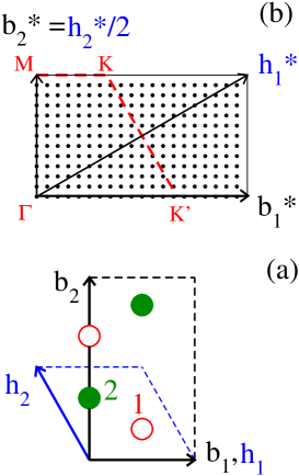
Figure 1: (a) The axes $(\mathbf{b}_{1},\mathbf{b}_{2})$ display a centered rectangular cell of a graphene layer containing four atoms. The primitive hexagonal axes are $(\mathbf{h}_{1,}\mathbf{h}_{2})$. There are 2 types of basis atoms, represented by closed and open circles, respectively. (b) The discrete $\mathbf{k}$-grid [see Eq. (17) ] used in the FT of Eq. (12) corresponding to a supercell $(\mathbf{a}_{1},\mathbf{a}_{2})=(20\mathbf{b}_{1},12\mathbf{b}_{2})$ is displayed by closed circles. $(\mathbf{b}_{1}^{*},\mathbf{b}_{2,}^{*})$ are the reciprocal basis vectors of the centered lattice, while $(\mathbf{h}_{1,}^{*},\mathbf{h}_{2,}^{*})$ are those of the primitive lattice. The reciprocal basis vectors of the simulation supercell are $(\mathbf{a}_{1}^{*},\mathbf{a}_{2}^{*})=(\mathbf{b}_{1}^{*}/20,\mathbf{b}_{2}^{*}/12).$ The points $\varGamma,M,K$, and $K^{\prime}$ are symmetry points at the boundary of the hexagonal BZ. The $\mathbf{k}$-points to the right of the $K-K^{\prime}$-line lie outside the first BZ. A translation by the reciprocal lattice vector $-\mathbf{h}_{1}^{*}=-(\mathbf{b}_{1}^{*}+\mathbf{b}_{2}^{*})$ moves these points within the first BZ.

It is now convenient to relabel the displacement coordinates of the $i^{\prime}$th atom to indicate the type of basis atom. Then the subindex $i$ ($i=1,\ldots N)$ will be replaced by a double subindex $\alpha j$,

$$(\mathbf{R}_{i},Z_{i})\longrightarrow(\mathbf{R}_{\alpha j},Z_{\alpha j})\equiv(X_{\alpha j},Y_{\alpha j,}Z_{\alpha j})\>,$$ (11)

where $\alpha$ ($\alpha=1,\ldots n)$ indicates that the $i^{\prime}$th atom belongs to the $\alpha^{\prime}$th basis subset, and $j$ ($j=1,\ldots,P_{c})$ is a running index for the $P_{c}$ symmetry equivalent atoms of the subset.

A symmetry adapted Bloch function, $\overline{X}_{\alpha}(\mathbf{k})$, is a collective variable defined as a linear combination of the mass-weighted displacement coordinates of the atoms within the $\alpha^{\prime}$th subset,(Kittel, 1966; Dove, 1993)

$$\overline{X}_{\alpha}(\mathbf{k})=\sqrt{\frac{m_{\alpha}}{P_{c}}}\sum_{j=1}^{P_{c}}X_{\alpha j}\exp\left(i\mathbf{k}\mathbf{r}_{eq,\alpha j}\right)\>.$$ (12)

$m_{\alpha}$ is the atomic mass of an atom in the $\alpha^{\prime}$th subset. The number of Bloch functions is $3n$, i.e., $\left[\overline{X}_{1}(\mathbf{k}),\overline{Y}_{1}(\mathbf{k}),\overline{Z}_{1}(\mathbf{k}),\ldots,\overline{X}_{n}(\mathbf{k}),\overline{Y}_{n}(\mathbf{k}),\overline{Z}_{n}(\mathbf{k})\right]$, that corresponds to the number of vibrational bands in the 2D solid. Note that the phase factor in the discrete Fourier transform (FT) is defined by the average crystal structure, $\left\{\mathbf{r}_{eq,\alpha j}\right\}$. This phase factor does not change when the coordinate $X_{\alpha j}$ is replaced by any other coordinate, $Y_{\alpha j}$ or $Z_{\alpha j}$, to derive the corresponding FT. The next (and nearly last) step is to calculate the hermitean susceptibility tensor, $\chi(\boldsymbol{\mathrm{k}})$.(Ramírez and López-Ciudad, 2001) Its $3n\times 3n$ elements are defined as ensemble averages of products of the form $\overline{A}_{\alpha}(\mathbf{k})\overline{B}_{\gamma}^{*}(\mathbf{k})$, with $\alpha$ and $\gamma$ as indices labeling basis atoms, and $A$ and $B$ as letters labeling any of the $(X,Y,Z)$ displacement coordinates. These products are the covariance of symmetry adapted functions of displacement coordinates. They provide a quantitative measure of the correlations in the atomic vibrations of the solid. A diagonal element of the tensor $\chi(\boldsymbol{\mathrm{k}})$ is derived as

$$\left\langle\overline{X}_{\alpha}(\mathbf{k})\overline{X}_{\alpha}^{*}(\mathbf{k})\right\rangle=S^{-1}\sum_{s=1}^{S}|\overline{X}_{\alpha}(\mathbf{k})|_{s}^{2}\>,$$ (13)

where $s$ is a running index for the simulation steps, and the vertical bars denote the modulus of the complex number. A non-diagonal element of $\chi(\boldsymbol{\mathrm{k}})$ is calculated as

$$\left\langle\overline{X}_{\alpha}(\mathbf{k})\overline{Y}_{\beta}^{*}(\mathbf{k})\right\rangle=S^{-1}\sum_{s=1}^{S}\left(\overline{X}_{\alpha}(\mathbf{k})\overline{Y}_{\beta}^{*}(\mathbf{k})\right)_{s}\>.$$ (14)

The last step is the diagonalization of the hermitean tensor $\chi(\boldsymbol{\mathrm{k}})$ that yields $3n$ real eigenvalues $\triangle_{j}(\mathbf{k})$. The eigenvectors of the tensor $\chi(\mathbf{k})$ are the Cartesian displacement vectors of the vibrational modes of the crystal, while the eigenvectors $\triangle_{j}(\mathbf{k})$ are a measure of the spatial dispersion of each mode. The one-body HLR result in Eq. (3), that relates the spatial dispersion $\delta X^{2}$ with the angular frequency $\omega$, can be generalized to the many-body problem to obtain the phonon dispersion bands $\omega_{j}(\mathbf{k})$ of the 2D solid as(Ramírez and López-Ciudad, 2001)

$$\omega_{j}^{2}(\mathbf{k})=\frac{1}{\beta\varDelta_{j}(\mathbf{k})}\>.$$ (15)

II.3 Treatment of reciprocal space

The reciprocal lattice vectors $(\mathbf{a}_{1}^{*},\mathbf{a}_{2}^{*})$ of the equilibrium simulation supercell are the columns of the matrix $\mathbf{S}$ defined as

$$\mathbf{S}=2\pi\left(\mathbf{\left\langle\Gamma\right\rangle}^{-1}\right){}^{T}\>,$$ (16)

so that $\mathbf{a}_{i}\mathbf{a}_{j}^{*}=2\pi\delta_{ij}$, with $\delta_{ij}$ as the Kronecker delta. The discrete FT in Eq. (12) is defined for $\mathbf{k}$-vectors that are commensurate with the simulation supercell, i.e.,

$$\mathbf{k}=k_{1}\mathbf{a}_{1}^{*}+k_{2}\mathbf{a}_{2}^{*}=(k_{1,}k_{2})\>.$$ (17)

The rhs gives the components of $\mathbf{k}$ using $(\mathbf{a}_{1}^{*},\mathbf{a}_{2}^{*})$ as basis vectors, with $k_{1}$ and $k_{2}$ being integers. If the simulation cell is defined as a $M_{1}\times M_{2}$ supercell of a crystallographic unit cell (either primitive or non-primitive), with $M_{1}$ and $M_{2}$ as positive integers, then $k_{1}$ and $k_{2}$ will vary between $0\leq k_{1}\leq M_{1}-1,$ and $0\leq k_{2}\leq M_{2}-1$.

For some applications it is convenient to convert the $\mathbf{k}$-grid of Eq. (17) into a symmetry equivalent one, that is located within the first BZ of the lattice. In the case that the crystallographic unit cell is a primitive one, the set of $\mathbf{k}$-vectors, $\mathbf{g}_{0}=(0,0)$, $\mathbf{g}_{1}=(M_{1,}0)$, $\mathbf{g}_{2}=(0,M_{2})$, and $\mathbf{g}_{3}=(M_{1},M_{2})$, are reciprocal lattice vectors of the primitive lattice. Then, the four vectors $\{\mathbf{k}-\mathbf{g}_{0}$, $\mathbf{k}-\mathbf{g}_{1}$, $\mathbf{k}-\mathbf{g}_{2}$, $\mathbf{k}-\mathbf{g}_{3}\}$ correspond to symmetry equivalent points in reciprocal space. Only one point of this set will belong to the first BZ. A sufficient condition for $\mathbf{k}$ to be located within the BZ is to choose the point whose vector modulus is the smallest, i.e.,

$$\mathbf{k}\equiv\mathrm{min\;mod}\left\{\mathbf{k}-\mathbf{g}_{0},\mathbf{k}-\mathbf{g}_{1},\mathbf{k}-\mathbf{g}_{2},\mathbf{k}-\mathbf{g}_{3}\right\}\>.$$ (18)

If the employed crystallographic unit cell is a non-primitive centered lattice, the vector from the set in Eq. (18) that is located within the first BZ is determined just by making a sketch in reciprocal space of the relative position of the grid of $\mathbf{k}$-vectors in Eq. (17) and the BZ of the primitive lattice. See Fig. 1 for a worked example of a graphene layer using a non-primitive centered rectangular cell.

III applications: graphene

The selected applications are intended as a test to illustrate the capability of the HLR approach in the calculation of phonon dispersion relations of 2D solids. Our main interest is to show the internal consistency of the HLR approach by comparing its predictions with other independent methods, and using a graphene monolayer as main example. Our vibrational analysis requires only spatial positions and it is equally applicable to classical and quantum simulations performed by either MD or MC methods. The fact that the HLR analysis can be applied indistinctly to either classical or quantum path integral simulations is an important feature of the method. To illustrate this capability, the selected applications of the HLR approach for graphene include both classical as well as path integral simulations.

III.1 Harmonic phonon dispersion in graphene

A simulation of the harmonic limit of an anharmonic potential must be performed in the classical low temperature limit. In the quantum case, anharmonic effects related to zero-point vibrations appear even in the $T\rightarrow 0$ limit.(Herrero and Ramírez, 2016) Under low temperature conditions, the agreement of the HLR phonon dispersion, $\omega(\mathbf{k}),$ and the harmonic result, $\omega_{H}(\mathbf{k})$, will serve as test of the HLR method. $\omega_{H}(\mathbf{k})$ is calculated, with independence from the simulation, by diagonalization of the vibrational dynamical matrix.(Kresse et al., 1995)

III.1.1 Computational conditions

The empirical long-range carbon bond order potential (LCBOPII) was employed in this calculation.(Los et al., 2005) In line with previous simulations a slight modification of the original torsion parameters was made to increase the bending constant of a flat layer in the $T\rightarrow 0$ limit from $\kappa=$0.82 eV to a more realistic value of $\kappa=$1.48 eV,(Ramírez et al., 2016; Tisi, 2017) closer to experimental data and ab-initio calculations.(Lambin, 2014) A temperature of 1 K and vanishing external stress ($P$=0) were chosen for the graphene MD simulation in the isotropic $NPT$ ensemble. The classical MD simulation was performed with a time step of 1 fs. The equilibration run consisted on $2\times 10^{6}$ MD steps (MDS) and a trajectory with 48000 layer configurations was stored at equidistant steps from a run with $2.4\times 10^{7}$ MDS. The stored trajectory was used to calculate the covariance of the atomic probability distributions by Eqs. (13) and (14). From a non-primitive centered rectangular graphene cell with 4 carbon atoms (see Fig. 1a), a $20\times 12$ supercell with $N=960$ atoms was defined for the graphene simulations. This rectangular supercell displays similar lengths in the $(x,y)$-directions. The dimension of the tensor $\chi(\mathbf{k})$ is $6\times 6$ for graphene. The shortest distance between points of the $\mathbf{k}$-grid of Eq. (17) is $\left|\mathbf{a}_{1}^{*}\right|\simeq\left|\mathbf{a}_{2}^{*}\right|=0.12$ Å^-1 (see Fig. 1b).

III.1.2 Phonon dispersion

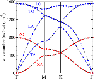
Figure 2: The harmonic phonon dispersion of graphene, $\omega_{H}(\mathbf{k}$), as derived by diagonalization of the dynamical matrix of the LCBOPII potential, is shown by dotted lines that look like solid lines when the slope is small. The six phonon bands are classified by their labels. The open circles are the HLR result as derived from the spatial atomic fluctuations obtained by a classical $NPT$ simulation with the same potential model. The MD simulation was performed close to the harmonic $T\rightarrow 0$ limit, at 1 K and $P=0$, on a $20\times 12$ supercell of a centered rectangular cell of graphene (see Fig. 1a). The $6\times 6$ susceptibility tensor $\chi(\mathbf{k})$ displays a block structure with separation of $(X,Y$) (blue circles) and $Z$ (red circles) bands.

The LCBOPII phonon dispersion of graphene, $\omega_{H}(\mathbf{k})$, derived from the diagonalization of the dynamic matrix, is presented in Fig. 2. The hexagonal cell parameter amounts to 2.4593 Å. The result corresponds to a dense set of points along the boundaries of the irreducible BZ (IBZ) of the hexagonal lattice. The dispersion relation of graphene comprises three acoustic (A) and three optical (O) bands, which are either in-plane longitudinal (L), in-plane transverse (T) or out-of-plane (Z). The acoustic ZA mode displays a $k^{2}$-dependence near $\mathit{\Gamma}$, in contrast with the linear dispersion of the TA and LA modes, which is typical for acoustic modes in 3D solids.(Zimmermann et al., 2008) The $\omega_{H}(\mathbf{k})$ bands in Fig. 2 (lines) are in agreement to previous calculations using the same LCBOPII model.(Locht, 2012)

The HLR result derived from the diagonalization of the $\chi(\mathbf{k})$ tensor are displayed as open circles in Fig. 2. The displayed $\mathbf{k}$-points correspond to those points in Eq. (17) that lie at the boundary of the IBZ. The agreement with the $\omega_{H}(\mathbf{k})$ dispersion is excellent for the six vibrational bands. The calculation of the tensor $\chi(\mathbf{k})$ includes the constraint provided by translational symmetry, but not from point symmetry elements of the crystal. Then, the symmetry of the vibrational modes will display errors associated to the finite sampling along the simulation. E.g., this error is about 0.3 % ($\sim$6 cm^-1) for the degenerate LO and TO modes at $\varGamma$. One could impose additional symmetry constraints (rotational axes and reflection planes) to the tensor $\chi(\mathbf{k})$ to ensure that the vibrational modes display the correct symmetry and smaller statistical errors. The reducible representation of the displacement vectors $(X_{\alpha j},Y_{\alpha j},Z_{\alpha j})$ of atoms in a solid is the same as that of atomic $p$-orbitals. Thus, the method to symmetrize $\chi(\mathbf{k})$ would be identical to that already used for the density matrices associated to $p$-orbitals in electronic band structure calculations based on crystal orbital methods.(Pisani and Dovesi, 1980; Ramírez and Böhm, 1988)

In the next Subsections, anharmonic shifts predicted by the HLR approach, caused by quantum zero-point motion and/or by an increase in temperature, are analyzed showing that they do lead to a consistent description of the collective vibrations.

III.2 Atomic kinetic energy in graphene

The vibrational kinetic energy of atoms in solids or molecules is a physical quantity that is affected by both quantum and anharmonic effects.(Ramírez and Herrero, 2011) The kinetic energy of the carbon atoms in graphene can be obtained by quantum PI simulations using the virial estimator. (Herman et al., 1982) This non-perturbative approach allows for an, in principle, “exact” treatment of both quantum and anharmonic effects as a function of temperature. This quantum observable is used to test the predictions of the HLR approach. In the classical limit, the vibrational kinetic energy amounts to $k_{B}T/2$ per degree of freedom (equipartition theorem), a value that does not depend on the anharmonicity of the interatomic potential.

III.2.1 Computational conditions

Quantum PIMD simulations of graphene with the LCBOPII model in the isotropic $NPT$ ensemble were performed at discrete temperatures between 25 and 750 K for an unstressed layer ($P=0$). The simulation cell with $N=960$ atoms is the same as that one described in Subsec. III.1. The Trotter number, $N_{Tr}$, that characterizes the applied discretization of the path integral was set as a temperature dependent value by the relation $N_{Tr}T=6000$ K. At 25 K, the lowest studied temperature, $N_{Tr}=240$, while at 750 K, the highest studied temperature, $N_{Tr}=8$. The time step was set as 0.5 fs, equilibration and simulations runs comprise $5\times 10^{5}$ MDS and $8\times 10^{6}$ MDS, respectively. At each temperature, the susceptibility tensor $\chi(\mathbf{k})$ was calculated from a set of $1.6\times 10^{4}$ crystal configurations stored at equidistant steps along the run. Further simulation conditions are identical to those already described in our previous PIMD graphene simulations.(Herrero and Ramírez, 2016, 2018)

III.2.2 Kinetic energy in the HLR approximation

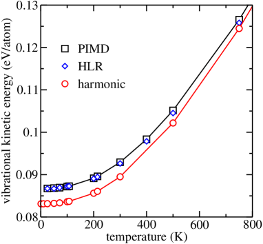
Figure 3: Vibrational kinetic energy of the carbon atoms in graphene as a function of temperature. The “exact” quantum PIMD result derived from the virial estimator (open squares) is compared to the approximation of Eq. (19) using the set of vibrational frequencies, $\omega(\mathbf{k})$, obtained either by the HLR approach (open diamonds) or in the harmonic approximation (open circles). The lines are guides to the eye.

The kinetic energy per atom, as derived from the PIMD simulation, is presented as a function of temperature in Fig. 3 as open squares. We observe that at low temperature the kinetic energy converges toward a constant zero-point value, while as temperature increases the thermal excitation of vibrational modes produces a gradual increase of the kinetic energy that tends to linearity in the high temperature limit.

The vibrational kinetic energy per atom can be estimated from the HLR frequencies, $\omega_{j}(\mathbf{k})$, derived by diagonalization of the susceptibility tensor, $\chi(\mathbf{k})$, as

$$E_{K}=\frac{1}{nN_{k}}\sum_{i=1}^{N_{k}}\sum_{j=1}^{3n}\frac{\hbar\omega_{j}(\mathbf{k}_{i})}{4}\coth\left(\frac{\beta\hbar\omega_{j}(\mathbf{k}_{i})}{2}\right)\>,$$ (19)

where the number of basis atoms is $n=2,$ and the number of $\mathbf{k}$-points is $N_{k}=$240 (as corresponds to the $20\times 12$ simulation supercell, see Subsec. II.3). Each mode of frequency, $\omega_{j}(\mathbf{k})$, is assumed to contribute to the kinetic energy by a quantum harmonic expression. Therefore anharmonicity in this model appears only in the value of the frequencies, $\omega_{j}(\mathbf{k})$, which may display shifts with respect to the harmonic limit. The HLR estimation of the kinetic energy is displayed in Fig. 3 as open diamonds. We observe an excellent agreement to the “exact” kinetic energy derived by the virial estimator at temperatures below 300 K. Anharmonic effects are present in the whole temperature range, but it is expected that they become larger as temperature rises. This might be the reason for the slight underestimation of the “exact” value of $E_{K}$ by the HLR approximation at the highest studied temperatures around 750 K. Even at this relatively high temperature, the kinetic energy in the classical limit ($3k_{B}T/2=0.097$ eV/atom) is significantly lower ($\sim$24%) than the value derived in the quantum approach.

The contribution of anharmonicity to the kinetic energy can be evaluated by calculation of the harmonic limit, $E_{KH}$, of the employed model potential. $E_{KH}$ is derived by replacing the HLR frequencies, $\omega_{j}(\mathbf{k})$, in Eq. (19) by harmonic ones, $\omega_{H,j}(\mathbf{k})$. The harmonic values, $\omega_{H,j}(\mathbf{k})$, which do not depend on temperature, were calculated by diagonalization of the dynamical matrix for a layer corresponding to the minimum potential energy (see Fig. 2). The harmonic kinetic energy, $E_{KH},$ shown as open circles in Fig. 3, differs appreciably from the “exact” $E_{K}$ in the whole temperature range. The anharmonic effect predicted by the LCBOPII model is an increase in the vibrational kinetic energy. The increase amounts to about $5\%$ at low temperatures, and is lower at higher temperatures ($\sim 2\%$ at 750 K). This behavior at high temperature is surely due to a compensation of errors, as anharmonic effects are expected to increase with temperature. The improved results of the HLR approach with respect to the harmonic limit reveal that the HLR frequencies are really sensitive to the anharmonic effect in the vibrational modes.

III.3 Temperature dependence of the optical phonons in graphene

III.3.1 LCBOPII model

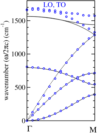
Figure 4: The HLR result for the phonon dispersion of graphene derived from a quantum PIMD simulation at 300 K is represented by open circles along $\Gamma-\mathrm{M}$. The dotted lines show the harmonic limit of the same model. The main anharmonic effect is a blue-shift of the LO and TO bands. These results were derived with the LCBOPII model.

The HLR phonon dispersion of graphene along the $\varGamma-M$ symmetry direction, derived from the quantum PIMD simulations at 300 K, is compared to the harmonic result in Fig. 4. We observe that the main anharmonic effect is a blue-shift of the LO and TO bands that amounts to $\sim 100$ cm^-1 ($\sim 6\%$) at the BZ center $\varGamma$. This anharmonic shift is the origin for the increase in the vibrational kinetic energy of the C atoms in the quantum PIMD simulation, in comparison to the quantum harmonic limit, as shown in Fig. 3. Nevertheless, this blue-shift seems to be an artifact of the LCBOP model, as it is in disagreement to both first-principles calculations(Bonini et al., 2007) and experimental results derived from Raman spectra.(Zhang et al., 2014)

An anharmonic blue-shift of the optical modes in graphene has been reported in three recent studies of the temperature dependence of its vibrational properties using either the LCBOP or LCBOPII potentials in classical MD simulations.(Koukaras et al., 2015; Anees et al., 2015; Tisi, 2017) The results of the LO/TO wavenumber of graphene at $\varGamma$ calculated in Ref. Tisi, 2017 from the Fourier transform of velocity time correlation functions with the LCBOPII model is displayed as a function of temperature in Fig. 5 (crosses). For comparison, the HLR result, as derived from classical simulations with the same potential model, is displayed as circles. A similar non-monotonic temperature dependence of the anisotropic shift of this optical mode is predicted by both methods, although there appear quantitative differences in the LO/TO wavenumbers, specially at high temperatures.

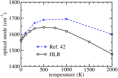
Figure 5: Temperature dependence of the degenerate LO/TO phonon wavenumber of graphene at $\varGamma$ as derived from classical simulations with the LCBOPII model. The results of Ref. Tisi, 2017, displayed by crosses, were derived from the Fourier transformed velocity time correlation functions. The results of the HLR analysis of classical MD simulations are given as open circles. Lines are guides to the eye.

III.3.2 Tight-binding model

We have re-analyzed the temperature dependence of the frequency of the degenerate LO and TO optical phonons of graphene at $\varGamma$ using an efficient tight-binding (TB) Hamiltonian parameterized using density-functional calculations,(Porezag et al., 1995) as an improved alternative to the LCBOPII model. The symmetry of this Raman active mode is $E_{2g}$ and corresponds to the G peak in the Raman spectra.(Ferrari and Basko, 2013)

Computational conditions:

Quantum and classical simulations of graphene were performed in the $NPT$ ensemble with isotropic volume fluctuations at $P=0$. The electronic structure has been treated with an efficient tight-binding (TB) Hamiltonian parameterized using density-functional calculations.(Porezag et al., 1995) The temperature was varied between 50 and 1000 K in the quantum PIMD simulations, and between 1 and 1000 K in the classical MD simulations. The time step was taken between 0.25 and 1 fs. The lowest time step of 0.25 fs was required for the quantum simulations at 50 K, where the atomic spatial delocalizations related to the zero-point quantum fluctuations are the largest. The simulation cell included 60 carbon atoms with periodic boundary conditions and the electronic energy was obtained using only the $\mathit{\Gamma}$-point for the calculation of the crystal band structure. The Trotter number, $N_{Tr}$, was set as a temperature dependent value by the relation $N_{Tr}T=6000$ K. Simulation runs comprise $8\times 10^{6}$ MDS and the analysis of the atomic real space fluctuations was performed on a subset of $1.6\times 10^{4}$ configurations stored equidistantly along the whole trajectory.

HLR analysis of the LO/TO phonons:

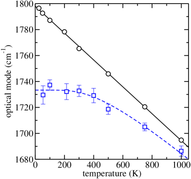
Figure 6: Temperature dependence of the $E_{2g}$ degenerate LO/TO vibrational states of graphene at $\varGamma$. This state corresponds to the G peak in the Raman spectrum. The results were derived by the HLR analysis of classical MD (open circles) and quantum PIMD (open squares) trajectories using a TB Hamiltonian. The continuous line is a linear fit of the classical result. The broken line is the least-squares fit of the quantum result to Eq. (20).

The temperature dependence of the optical LO and TO vibrational modes at $\varGamma$ as derived from the HLR method is displayed in Fig. 6. In the classical limit the optical mode display a linear temperature dependence. The classical $T\rightarrow 0$ limit corresponds to the harmonic expectation, $\omega_{H}=1798$ cm^-1 , for the TB model under the employed computational conditions. This value overestimates by about 12% the experimental value.(Zhang et al., 2014) Vibrational frequencies determined from ab-initio calculations are often scaled by empirical factors to compensate for systematic biases that overestimate frequencies by about 10% (e.g. in Hartree-Fock 6-31G(d) models).(Irikura et al., 2005)

In the classical limit, the change of the optical mode frequency with temperature is given by a slope of $\varphi_{T}=-0.1$ cm^-1/K. The negative sign of the slope indicates that the anharmonicity of the optical modes predicted by the TB method is indeed a red-shift of the vibrational frequency, as opposed to the results derived previously for the LCBOPII model. The quantum results for the temperature dependence of this optical mode differ from the classical ones, specially below room temperature. The intrinsic anharmonicity of the zero-point vibration of the carbon atoms makes that the optical modes display a shift of $\sim-64$ cm^-1 with respect to the classical expectation in the low temperature limit.

Temperature-dependent Raman scattering experiments have shown that the temperature variation of the phonon line center can be attributed to the anharmonicity in the vibrational potential, which leads to the decay of optical phonons into low-energy acoustic phonons. The effect of this decay on the frequency of the optical modes at $\varGamma$ has been described by the expression(Anand et al., 1996)

$$\Delta\omega(T)=\omega(T)-\omega_{0}=C\left(1+\frac{2}{\exp\left[\hbar\omega_{0}/2k_{B}T\right]-1}\right)\>,$$ (20)

where $\omega_{0}$ is the intrinsic frequency of the optical phonon, i.e., $\omega_{0}\equiv\omega_{H}(T\rightarrow 0)=1798$ cm^-1, and $C$ is the anharmonic constant. The least-squares fit of the HLR results to Eq. (20) is shown in Fig. 6. The anharmonic constant amounts to $C=-64.7$ cm^-1. At 300 K the temperature coefficient $\varphi_{T}=-0.026$ cm^-1/K derived from the quantum simulation is about 5 times smaller that the classical prediction. The quantum result is in excellent agreement with the temperature coefficient derived from Raman measurements for single-walled carbon nanotubes with a wide range of diameters,(Zhang et al., 2007) although the diameter of the nanotube did not have any obvious influence on the value of $\varphi_{T}.$ The experimental average value over nanotubes of different diameters was $\varphi_{T}=-0.026$ cm^-1/K, a value which was also obtained in subsequent Raman investigations.(Zhang et al., 2014)

III.4 Temperature dependence of elastic moduli in graphene

The temperature dependence of the elastic moduli is another important anharmonic effect,(Katsnelson, 2005) that will be analyzed in graphene by the HLR approach.

III.4.1 Computational conditions

Classical MD simulations of graphene in the isotropic $NPT$ ensemble were performed with the LCBOPII model at discrete temperatures between 1 and 1000 K for an unstressed layer ($P=0$). The simulation cell with $N=960$ atoms was the same as that one described in Subsec. III.1. The time step was set as 1 fs. Two sets of simulations were performed. In the first one, the carbon atoms move unconstrained along trajectories with $2.4\times 10^{7}$ MDS. In the second set, the carbon atoms moved along trajectories with $8\times 10^{6}$ MDS in the $(x,y)$-plane (the atomic $z$-coordinate is constraint as $z=0$) . The acoustic LA and TA phonon dispersions (see Fig. 2) were derived by a HLR analysis of the trajectories. The slopes of the acoustic TA and LA phonons of graphene in the long-wavelength limit ($k\rightarrow 0$) (see Fig. 2) correspond to the sound velocities $v_{T}$ and $v_{L}$. They were determined by a least-squares fit of the corresponding phonon dispersion bands using the function

$$\omega=\left(v^{2}k^{2}+ck^{4}\right)^{1/2}\>,$$ (21)

where $v$ is the sound velocity and $c$ is a fitting constant. Only those $\mathbf{k}$-points with modulus $k<0.43$ Å^-1 were included in the fit.

III.4.2 Elastic moduli from the HLR analysis

The sound velocities of the acoustic (TA and LA) phonons of 2D layers provide information on its elastic moduli. The sound velocities of the TA and LA branches for an isotropic 2D elastic media are(Cottam, 2015)

$$v_{T}=\left(\frac{\mu}{\rho}\right)^{1/2}\>,$$ (22)

$$v_{L}=\left(\frac{B^{\prime}}{\rho}\right)^{1/2}\>.$$ (23)

where $\rho$ is the in-plane mass density, $\mu$ is the shear modulus (Lam ’s second coefficient), and $B^{\prime}$ is the unilateral compressional modulus defined as,(Behroozi, 1996)

$$B^{\prime}=\lambda+2\mu\>,$$ (24)

where $\lambda$ is the Lam ’s first coefficient.(Behroozi, 1996) The in-plane compressional modulus (the 2D analogous to the bulk modulus) is derived from $\mu$ and $B^{\prime}$ as(Behroozi, 1996)

$$B=B^{\prime}-\mu=\lambda+\mu\>.$$ (25)

The temperature dependence of the elastic moduli, $\mu$ and $B^{\prime}$ of graphene, as derived from the HLR analysis are presented in Fig. 7 as open circles. In the strictly flat 2D layer ($z=0$ for the C atoms, Fig. 7b) the shear modulus $\mu$ is nearly temperature independent, while the moduli $B^{\prime}$ and $B$ decrease slightly with temperature.

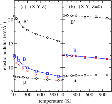
Figure 7: Temperature dependence of elastic moduli of graphene as derived from the HLR analysis of classical MD simulations. Open circles are results for $\mu$ and $B^{\prime}$ derived from a least-squares fit of the phonon dispersion curves. Open squares are the estimation of the in-plane stiffness as $B=B^{\prime}-\mu$. The crosses are values of $B$ from the fluctuation formula in Eq. (26). Lines are guides to the eye. Panel (a) shows results of simulations where the layer atoms move without constraints in the $(x,y,z)$ space. In Panel (b) the carbon atoms move in the $(x,y)$-plane with the constraint $z=0$. The results were derived with the LCBOPII model.

It is interesting to compare the HLR result for the compressional modulus, $B$ (open squares in Fig. 7b), to the value calculated by the fluctuation formula in the $NPT$ ensemble,(Landau and Lifshitz, 1980; Ramírez and Herrero, 2017)

$$B=\frac{V}{N\beta\delta V^{2}}\>,$$ (26)

where $V$ denotes the average in-plane area per atom that fluctuates in the $NPT$ ensemble with dispersion $\delta V^{2}$. The values of $B$ derived from this equation are presented by crosses in Fig. 7b. Within the statistical error of the simulations, the values of $B$ by the HLR analysis are in good agreement with the fluctuation formula.

The results for $B^{\prime}$, $\mu$, and $B$ as derived by the HLR analysis when the atoms of the layer move without constraint are displayed in Fig. 7a. The atomic out-of-plane vibrations have a significant influence in the elastic moduli of the layer, that display a more pronounced temperature dependence than in Fig. 7b. A striking result is that the HLR values of the in-plane compressional modulus $B$ (open squares) are now systematically larger than those derived from the fluctuation formula (crosses) in Fig. 7a. The atomic displacements in the out-of-plane direction, causing the spatial corrugation of the 2D layer, must be the origin of this unexpected behavior.

Several plausible effects may explain the fact that Eqs. (25) and (26) give different results for a 2D layer fluctuating in 3 dimensions. One possibility is that the anharmonicity of the out-of-plane displacements is not correctly reproduced by the HLR analysis. However, any anharmonic effect in a classical simulation should decrease gradually with temperature and eventually vanish in the low temperature limit, a behavior that is not supported by the results of Fig. 7a.

A second possibility is that the disagreement between the results derived from Eqs. (25) and (26) is a finite size effect related to the out-of-plane vibrations. We have checked the finite size effect at 300 K by increasing the cell size from $N=960$ to $N=8400$ atoms. The size effect reduces the value of $B$. However, the decrease derived from the HLR phonon dispersion relations is lower ($\sim 21\%$) than that derived from the fluctuation formula ($\sim 27\%$). Thus, this effect would make the disagreement found between both results even larger.

An intriguing explanation for the disagreement in the results of $B$ in Fig. 7a and the agreement in Fig. 7b, is that when the 2D layer fluctuates in the $z$-direction, forming ripples and loosing its strictly 2D character, the in-plane compressional modulus $B$ in Eq. (25) becomes different than that one in Eq. (26). Ripples depend on an additional elastic modulus, the bending stiffness, $\kappa$, that for an atom thick layer is a constant independent from the Lam coefficients, $\lambda$ and $\mu$.

IV Applications: graphene bilayer and graphane

Examples of the application of the HLR approach to 2D layers different from graphene monolayer is illustrated for a graphene bilayer and for chair-graphane.

IV.1 Harmonic phonon dispersion in a graphene bilayer

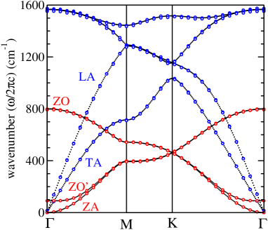
Figure 8: The harmonic phonon dispersion of bilayer graphene with stacking AB, as derived from the dynamical matrix of the LCBOPII model, is shown by dotted lines that look like solid lines when the slope is small. Open circles represent the HLR result as derived from a classical $NPT$ simulation using the same model. The MD simulation was performed close to the harmonic $T\rightarrow 0$ limit, at 1 K and $P=0$, using a supercell with $N=1920$ atoms. The $12\times 12$ susceptibility tensor $\chi(\mathbf{k})$ displays a block structure with separation of $(X,Y)$ (blue circles) and $Z$ (red circles) bands.

A classical MD $NPT$ simulation of a graphene bilayer with AB stacking has been performed at $T=1$ K and $P=0$ with similar computational conditions as those employed for graphene in the previous Subsec. III.1. The hexagonal cell parameter with the employed LCBOPII model amounts to 2.4584 Å, while the interlayer distance is 3.3372 Å. The simulation cell includes two atomic layers adding up $N=1920$ atoms. The dimension of the tensor $\chi(\mathbf{k})$ is $12\times 12$ for the bilayer. A comparison of the harmonic dispersion curves, $\omega_{H}(\mathbf{k})$, with those derived by the HLR approach is presented in Fig. 8. We find that the agreement between both methods is excellent for the 12 vibrational bands.

All vibrational bands of bilayer graphene, except ZA (see Fig. 8), appear as degenerate at the scale of the figure. The ZA band of graphene is splitted into ZA and ZO’ bands in the bilayer. The larger splitting is found at $\varGamma$ where the frequency of the ZO’ mode amounts to 91 cm^-1 (see Fig. 8). This is the layer breathing mode, where the $z$-distance between the two graphene layers oscillates around its equilibrium value. The acoustic LA and TA modes of graphene also split in the bilayer, but the splitting is too small to be seen in Fig. 8. The largest splitting is again found at $\varGamma$ and amounts to 15 cm^-1. This vibrational mode of the bilayer corresponds to a rigid layer shear mode, involving the relative motion of atoms in adjacent planes. Raman spectroscopy of a graphene bilayer gives a frequency of 32 cm^-1 for this rigid layer shear mode,(Tan et al., 2012) while the ZO’ breathing mode appears at 89 cm^-1 at $\varGamma$.(Lin et al., 2018) The splitting of the LO and TO modes at $\varGamma$ is even smaller, less that 1 cm^-1 with the LCBOPII model. The splitting obtained with density-functional perturbation theory amounts to 5 cm^-1.(Yan et al., 2008)

IV.2 Vibrational anharmonic effects in chair-graphane

IV.2.1 Computational conditions

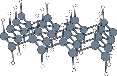
Figure 9: 2D structure of chair-graphane. Carbon and hydrogen atoms are represented by circles, the smaller ones correspond to H.

The 2D layer structure of chair-graphane is displayed in Fig. 9. The electronic structure has been treated with the TB electronic band structure method of Subsec. III.3. The hexagonal cell displays a cell parameter of 2.5320 Å, and the vertical atomic distances to the mean layer plane are 0.2319 Å for C and 1.3576 Å for H. Classical MD simulations with the isotropic $NPT$ ensemble were performed on a $6\times 4$ supercell of a centered rectangular cell containing $N=192$ atoms, at external stress $P=0$, and temperatures of $T=1$ K and $T=300$ K. Only the $\varGamma$ point for the sampling of the BZ of the simulation supercell was used in the electronic structure calculation. The equilibration run consisted on $2\times 10^{5}$ MDS and a trajectory with 10000 layer configurations was stored at equidistant steps from a run with $2\times 10^{6}$ MDS. The classical MD simulation was performed with a time step of 1 fs.

IV.2.2 Phonon dispersion

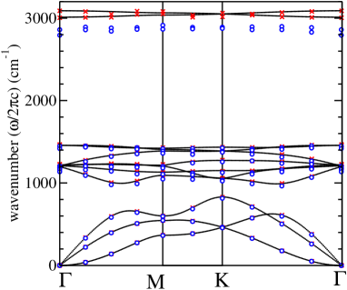
Figure 10: The harmonic phonon dispersion of chair-graphane, as calculated from the dynamical matrix of the employed TB model, is shown by lines. HLR wavenumbers derived from classical $NPT$ simulations with the same TB model at $P=0$, using a supercell with $N=192$ atoms, are shown at temperatures of 300 K (open circles) and 1 K (crosses). A significant anharmonic red-shift is visible in the bands associated to the C$-$H stretching vibrations at frequencies around 2850 cm${}^{-1}.$ The HLR results for the other vibrational bands at 300 K and at 1K are nearly indistinguishable at the scale of the figure.

The harmonic phonon dispersion of chair-graphane, as derived from the dynamical matrix of the employed TB model, is displayed in Fig. 10 (lines). There appear 12 dispersion bands. The two flat dispersion bands around 3000 cm^-1 correspond to the stretching of the C$-$H bonds along the $z$-direction perpendicular to the layer. The general appearance of the TB harmonic dispersion bands show reasonable agreement to previous calculations by first-principles electronic structure calculations.(Cadelano et al., 2010; Peelaers et al., 2011) The result of the HLR analysis of a classical graphane simulation at 1 K, displayed in Fig. 10 (crosses), is identical, within the statistical error of the simulation, to the harmonic dispersion bands.

Anharmonic effects due to the increased amplitude of atomic vibrations are expected to appear as the temperature rises. Therefore, at 300 K deviations of the HLR phonon dispersion from the harmonic limit indicate the presence of anharmonic effects in the corresponding vibrational modes. The HLR phonon dispersion curves at 300 K is displayed by open circles in Fig. 10. The most significant anharmonic effect is a red-shift of the bands associated to the stretching of the C$-$H bonds by about 150 cm^-1, while anharmonic effects in the rest of vibrational bands are comparatively low. For many organic molecules, the anharmonicity of C–H modes is estimated to red-shift the harmonic stretching frequency by about 120–140 cm^-1.(Gentile et al., 2017)

V Summary

We have presented the HLR method as a tool to study the phonon dispersion relations of 2D layers from the analysis of trajectories generated by equilibrium MD or MC simulations, either with the quantum PI formalism, or in the classical limit. The HLR method is based on the analysis of the spatial correlations of centroid or atomic displacements by means of the diagonalization of the covariance matrices associated to these displacements. The HLR method for 2D layers could be straightforwardly applied to 1D or 3D solids. The only difference is that in the Fourier transform of Eq. (12) the dimension of the $\mathbf{r}_{eq}$- and $\mathbf{k}$-vectors will depend on the the dimensionality of the problem.

The physical information needed in the HLR method is the static susceptibility tensor, $\chi(\mathbf{k})$, that defines the linear response of an equilibrium system to static forces. As the linear response of the system depends on the anharmonicity of the interatomic potential, anharmonic effects are included in the HLR approach in a realistic way.

By means of classical MD simulations at very low temperatures, we have checked that the HLR approach reproduces the harmonic phonon dispersion relations obtained by diagonalization of the dynamical matrix. This test has been presented for several 2D systems: a graphene monolayer, a graphene bilayer, and a graphane monolayer. The sensitivity of the HLR approach to reproduce anharmonic effects has been demonstrated by the calculation of the temperature dependence of the atomic kinetic energy of carbon atoms in graphene by quantum PIMD simulations. Anharmonic shifts in the optical phonon frequencies of graphene have been derived by the HLR method. The comparison of the quantum results and the classical limit display the significant anharmonicity of the zero-point vibrations. Another studied anharmonic effect is the temperature dependence of the elastic moduli of graphene. An intriguing difference has been found in alternative ways to calculate the in-plane compressional modulus of a graphene layer, either by the HLR phonon dispersion curves or by the fluctuation of the area in the isothermal-isobaric ensemble. Both methods provide identical result for a strict 2D planar layer, but display a systematic difference in the presence of out-of-plane fluctuations of the layer.