TU–1094

KYUSHU–HET–205

On renormalons of static QCD potential at $u=1/2$ and $3/2$

Yukinari Sumino^a and Hiromasa Takaura^b
aDepartment of Physics, Tohoku University,
Sendai, 980-8578 Japan
^bDepartment of Physics, Kyushu University,
Fukuoka, 819-0395 Japan

We investigate the $u=1/2$ [${\cal O}(\Lambda_{\rm QCD})$] and $u=3/2$ [${\cal O}(\Lambda_{\rm QCD}^{3})$] renormalons in the static QCD potential in position space and momentum space using the OPE of the potential-NRQCD effective field theory. This is an old problem and we provide a formal formulation to analyze it. In particular we present detailed examinations of the $u=3/2$ renormalons. We clarify how the $u=3/2$ renormalon is suppressed in the momentum-space potential in relation with the Wilson coefficient $V_{A}(r)$. We also point out that it is not straightforward to subtract the IR renormalon and IR divergences simultaneously in the multipole expansion. Numerical analyses are given, which clarify the current status of our knowledge on the perturbative series. The analysis gives a positive reasoning to the method for subtracting renormalons used in recent $\alpha_{s}(M_{Z})$ determination from the QCD potential.

1 Introduction

For a long time the static QCD potential ${V}_{\rm QCD}(r)$ has been studied extensively, in order to understand the nature of the strong interaction between a heavy quark and antiquark pair. In the past decades computation of ${V}_{\rm QCD}(r)$ in perturbative QCD has been advanced significantly [1, 2, 3, 4, 5, 6, 7, 8, 10, 11, 12, 13, 14, 15, 16, 17]. In association with many theoretical developments, ${V}_{\rm QCD}(r)$ has become an indispensable theoretical tool to describe not only the properties of the heavy quarkonium states but also for precision determinations of the fundamental parameters of QCD such as the heavy quark masses $m_{c}$, $m_{b}$, $m_{t}$ [18, 19, 20, 21, 22, 23, 24, 25, 26, 27] and the strong coupling constant $\alpha_{s}$ [28, 29].

Before around 1998, the prediction of ${V}_{\rm QCD}(r)$ in perturbative QCD was not successful and was plagued by the so-called renormalon problem. As it turned out, convergence of the perturbative series was fairly poor, such that a meaningful prediction could not be obtained in the distance regions relevant to the charmonium and bottomonium states. This is caused by the growth of $\alpha_{s}$ in the infrared (IR) region and is characterized by the singularities in the Borel transform of the perturbative series (the singularities are called renormalons) [30]. Then it was discovered that the leading renormalon of order $\Lambda_{\rm QCD}$ in ${V}_{\rm QCD}(r)$ is canceled against that of the quark pole mass $m_{\rm pole}$ in the combination of the total energy of the static quark pair $2m_{\rm pole}+{V}_{\rm QCD}(r)$, which led to a dramatic improvement of convergence of the perturbative series [31, 32, 33].

Up to now, although there exists no rigorous proof on existence of renormalons in QCD observables, there exist standard arguments based on the operator product expansion (OPE) and renormalization group (RG) equations which show that their existence is consistent and plausible theoretically [30]. This is reinforced by a number of evidences in actual computation of perturbative series of QCD observables, thanks to recent technological developments in multiloop calculations. There also exist examinations of the nature of renormalons using many approximate estimates of higher-order terms of perturbative series at various levels of rigor. See, for instance, Ref. [34].

In many analyses of renormalons in the static QCD potential, analyses of perturbative computation in momentum space play important roles [30]. For ${V}_{\rm QCD}(r)$, it is often assumed that there are no renormalons in its Fourier transform $\widetilde{V}_{\rm QCD}(q)$ (the potential in momentum space) or that renormalons in $\widetilde{V}_{\rm QCD}(q)$ are negligible at the current level of accuracy. In fact, in Refs. [32] and [33], absence of the order $\Lambda_{\rm QCD}/q^{3}$ renormalon in $\widetilde{V}_{\rm QCD}(q)$ (corresponding to the $u=1/2$ renormalon) is shown at the one-loop and two-loop levels, respectively. Also, the $u=3/2$ renormalon cancellation within the multipole expansion was shown [9] based on the assumption of absence of the corresponding renormalon in $\widetilde{V}_{\rm QCD}(q)$. Nevertheless, it can be the case that renormalons arise from a deep level of loop integrals in the computation of $\widetilde{V}_{\rm QCD}(q)$ and that they are simply not detected in the currently known several terms of the perturbative series.

A direct motivation of our study comes from necessity for a justification for the assumption used in a recent determination of $\alpha_{s}$ from ${V}_{\rm QCD}(r)$ [29]. There, the first two renormalons of order $\Lambda_{\rm QCD}$ and $\Lambda_{\rm QCD}^{3}r^{2}$ are subtracted from the leading-order Wilson coefficient of ${V}_{\rm QCD}(r)$, in order to extend validity range of the OPE of ${V}_{\rm QCD}(r)$ to larger $r$, and it is assumed that the corresponding renormalons are negligible in the Fourier transform of the Wilson coefficient [$\simeq\widetilde{V}_{\rm QCD}(q)$]. This problem is also linked with how we renormalize the IR divergences in the potential which arise from three loops and beyond [2, 8, 10, 15, 16, 11].

In this paper we analyze the order $\Lambda_{\rm QCD}$ and $\Lambda_{\rm QCD}^{3}r^{2}$ renormalons in ${V}_{\rm QCD}(r)$, on the basis of the standard argument by the OPE and RG equations. The discussion is to a large extent based on general features of QCD, independent of ad hoc approximations such as the large-$\beta_{0}$ approximation. We refine our understanding by looking into the detailed structure of the OPE within the potential-NRQCD (pNRQCD) effective field theory (EFT) [35]. In particular we elucidate the accurate structure of the $u=3/2$ renormalon. Subsequently we discuss the size of the renormalon uncertainties for $u=1/2$ and $3/2$ in $\widetilde{V}_{\rm QCD}(q)$ with a method which does not rely on diagrammatic analysis, providing a different perspective from, e.g., Refs. [33, 9]. We also believe that an argument such as the one we provide in Sec. 3 is necessary to clarify treatment of the IR part of $\widetilde{V}_{\rm QCD}(q)$. In the latter part of this paper, we test our understanding by performing numerical analyses of the normalization constants of the renormalons in the perturbative series of ${V}_{\rm QCD}(r)$ and $\widetilde{V}_{\rm QCD}(q)$. We treat two kinds of perturbative series: one is the fixed-order perturbative series currently known and the other includes higher-order terms estimated by RG. We estimate the normalization constants of the renormalons from these two perturbative series by using Lee’s method [36] and also by an analytic formula which we derive (for the latter series). The former includes updates of the analyses by Pineda [37]. See also Ref. [18] for a more recent result.

The paper is organized as follows. In Sec. 2 we briefly review the standard argument on renormalons for a general QCD observable. In Sec. 3 we scrutinize the structure of renormalons in the static QCD potential. Secs. 4–8 present numerical analyses on the normalization constants of the renormalons. In Sec. 4 we study the ${\cal O}(\Lambda_{\rm QCD})$ renormalon of ${V}_{\rm QCD}(r)$ from fixed-order perturbative series, followed by a study of its cancellation with that of the pole mass in Sec. 5. We compare these results with that obtained by an integral formula in Sec. 6. We study the ${\cal O}(\Lambda_{\rm QCD}^{3}r^{2})$ renormalon of ${V}_{\rm QCD}(r)$ in Sec. 7. Finally we test the corresponding renormalons in $\widetilde{V}_{\rm QCD}(q)$ in Sec. 8. Conclusions are given in Sec. 9. In App. A we explain theoretical aspects of IR cancellation at $O(r^{0})$ of the multipole expansion. In App. B we present details of the derivation of a formula for the normalization of renormalons in ${V}_{\rm QCD}(r)$.

2 Structure of renormalons

Let us first review briefly the structure of renormalons in QCD observables [30].

Consider a general RG-invariant dimensionless observable $X(Q)$ with a typical energy scale $Q$. Its perturbative expansion is given by

$$X^{\rm PT}(Q)=\sum_{n=0}^{\infty}d_{n}(Q/\mu)\alpha_{s}(\mu)^{n+1}\,.$$ (1)

$\mu$ denotes the renormalization scale in the $\overline{\rm MS}$ scheme. It satisfies the RG equation

$$\mu^{2}\frac{d}{d\mu^{2}}X^{\rm PT}(Q)=\left[\mu^{2}\frac{\partial}{\partial\mu^{2}}+\beta(\alpha_{s})\frac{\partial}{\partial\alpha_{s}}\right]X^{\rm PT}(Q)=0$$ (2)

with the beta function given by

$$\mu^{2}\frac{d\alpha_{s}}{d\mu^{2}}=\beta(\alpha_{s})=-\sum_{i=0}^{\infty}b_{i}\,\alpha_{s}^{i+2}\,.$$ (3)

The first two coefficients of the beta function are given explicitly by

$$b_{0}=\frac{1}{4\pi}\left(11-\frac{2}{3}n_{f}\right),~{}~{}~{}~{}~{}b_{1}=\frac{1}{(4\pi)^{2}}\left(102-\frac{38}{3}n_{f}\right)\,.$$ (4)

It is conjectured that for many observables the coefficients of the perturbative series grow factorially, $d_{n}\sim n!$, for large $n$. To quantify uncertainties induced by this property, the Borel transform of $X^{\rm PT}$, defined by

$$B_{X}(t)=\sum_{n=0}^{\infty}\frac{d_{n}}{n!}t^{n}\,,$$ (5)

is studied. Renormalons of $X^{\rm PT}$ refer to the singularities of $B_{X}(t)$ located on the real axis in the complex $t$-plane. We assume the form of the Borel transform in the vicinity of each renormalon singularity at $t=u/b_{0}$ as

$$B_{X}(t)=\left(\frac{\mu^{2}}{Q^{2}}\right)^{u}\frac{N_{u}}{\displaystyle\bigl{(}1-{b_{0}t}/{u}\bigr{)}^{1+\nu_{u}}}\,\sum_{k=0}^{\infty}c_{k}(\mu/Q)\left(1-\frac{b_{0}t}{u}\right)^{k}+\text{(regular part)}\,,$$ (6)

$$c_{0}=1\,,$$ (7)

with parameters $N_{u}$, $\nu_{u}$ and $c_{k}$’s. This form is consistent with the RG equation. Formally we can reconstruct $X^{\rm PT}$ from its Borel transform $B_{X}(t)$ by the inverse Borel transform given by the integral

$$X^{\rm PT}``="\int_{0}^{\infty}dt\,B_{X}(t)e^{-t/\alpha_{s}(\mu)}\,.$$ (8)

However, if there are singularities (renormalons) on the positive real axis, the integral is ill defined. We can regularize the integral by deforming the integral contour to the upper or lower half plane:

$$X_{\pm}^{\rm PT}=\int_{0}^{\infty\times\exp(\pm i\epsilon)}dt\,B_{X}(t)e^{-t/\alpha_{s}(\mu)}\,.$$ (9)

We can define the ambiguity induced by the renormalon from the discontinuity of the corresponding singularity, and the singularity at $t=u/b_{0}$ with $u>0$ of eq. (6) gives

$${\rm Im}\,X^{\rm PT}_{\pm}[u]=\pm\frac{\pi}{b_{0}}\frac{N_{u}}{\Gamma(1+\nu_{u})}u^{1+\nu_{u}}\left(\frac{\Lambda_{\overline{\rm MS}}^{2}}{Q^{2}}\right)^{u}(b_{0}\alpha_{s}(Q))^{-\nu_{u}+ub_{1}/b_{0}^{2}}\sum_{k=0}^{\infty}\tilde{c}_{k}\alpha_{s}(Q)^{k}\,,$$

$$~{}~{}\tilde{c}_{0}=1\,,$$ (10)

where we have used

$$\Lambda_{\overline{\rm MS}}^{2}=\mu^{2}\,\exp\left[-\left\{\frac{1}{b_{0}\alpha_{s}}+\frac{b_{1}}{b_{0}^{2}}\log(b_{0}\alpha_{s})+\int_{0}^{\alpha_{s}}\!dx\,\left(\frac{1}{\beta(x)}+\frac{1}{b_{0}x^{2}}-\frac{b_{1}}{b_{0}^{2}x}\right)\right\}\right]\,.$$ (11)

The parameters $u$, $\nu_{u}$, $c_{k}$ and $\tilde{c}_{k}$ in eq. (6) or eq. (10) can usually be determined from the OPE. In the context of the OPE in $1/Q$, $X^{\rm PT}$ is identified with the Wilson coefficient of the leading identity operator. Let us denote by $O_{u}$ the lowest dimension (dimension $2u$) renormalized operator responsible for cancellation of the leading renormalon in $X^{\rm PT}$. For simplicity we discuss the case where only one operator is involved. The OPE reads

$$X(Q)=C_{1}^{X}(Q)+C^{X}_{O_{u}}(Q/\mu,\alpha_{s}(\mu))\frac{\left<{0}\,\right|O_{u}(\mu)\left|\,{0}\,\right>}{Q^{2u}}+\cdots\,,$$ (12)

$$C^{X}_{1}(Q)=X^{\rm PT}(Q)\,,~{}~{}~{}C^{X}_{O_{u}}(Q/\mu,\alpha_{s}(\mu))=\sum_{n=0}^{\infty}f_{n}(Q/\mu)\alpha_{s}(\mu)^{n}\,.$$ (13)

We assume that the leading ambiguity induced by the renormalon of $C_{1}^{X}$ as given in eq. (10) is canceled by the second term of the OPE. Then, the $Q$-dependence of the renormalon uncertainty of $C_{1}^{X}$ should coincide with that of the second term in the OPE, which can be detected as follows. Suppose that the Wilson coefficient satisfies the RG equation,

$$\left[\mu^{2}\frac{d}{d\mu^{2}}-\gamma(\alpha_{s})\right]C_{O_{u}}^{X}=0~{}~{}~{};~{}~{}~{}\gamma(\alpha_{s})=\sum_{i=0}^{\infty}\gamma_{i}\,\alpha_{s}^{i+1}\,.$$ (14)

This RG equation specifies the $Q$-dependence of $C^{X}_{O_{u}}(Q/\mu,\alpha_{s}(\mu))$ as

$$C_{O_{u}}^{X}(Q/\mu,\alpha_{s}(\mu)) =\exp\left[-\int_{\alpha_{s}(\mu)}^{\alpha_{s}(Q)}dx\,\frac{\gamma(x)}{\beta(x)}\right]C_{O_{u}}^{X}(1,\alpha_{s}(Q))$$

$$=const.\times[\alpha_{s}(Q)]^{\gamma_{0}/b_{0}}[1+\mathcal{O}(\alpha_{s}(Q))]C_{O_{u}}^{X}(1,\alpha_{s}(Q))\,,$$ (15)

where $const.$ denotes a $Q$-independent (but $\mu$-dependent) constant. Now the $Q$-dependence of the second term of the OPE (12) is made explicit.

Requiring the same $Q$-dependence for the renormalon uncertainty of $X^{\rm PT}$, using eq. (12) with eq. (15), we obtain for eq. (6) or (10)

$$\nu_{u}=\frac{b_{1}}{b_{0}^{2}}u-\frac{\gamma_{0}}{b_{0}}\,.$$ (16)

The factor $\sum_{k=0}^{\infty}\tilde{c}_{k}\alpha_{s}(Q)^{k}$ in eq. (10) should be proportional to $[1+\mathcal{O}(\alpha_{s}(Q))]C_{O_{u}}^{X}(1,\alpha_{s}(Q))$ in eq. (15). Therefore, $c_{k}$’s and $\tilde{c}_{k}$’s can be determined one by one from smaller $k$ in terms of $b_{n}$’s, $\gamma_{n}$’s and $f_{n}$’s from smaller $n$. The overall normalization $N_{u}$ cannot be determined from this argument. We note that, in the case that $C^{X}_{O_{u}}O_{u}$ is independent of $Q$, $\gamma_{0}=0$ and $\tilde{c}_{k}=0$ for $k\geq 1$.

3 Renormalons in the static QCD potential

In this section we investigate theoretical aspects of renormalons of the static QCD potential, focusing on the $u=1/2$ and $3/2$ renormalons, on the basis of the above general understanding. Part of the argument given in this section has already been discussed in [8]. (See also [38].) We refine the discussion and present new observations. In particular, main part of the discussion on the $u=3/2$ renormalon is new.

3.1 Basics of static QCD potential

The static QCD potential is defined from an expectation value of the Wilson loop as

$$V_{\rm QCD}(r)=-\!\lim_{T\to\infty}\frac{1}{iT}\,\log\frac{\left<{0}\,\right|{\rm{Tr\,P}}\exp\left[ig\oint_{C}dx^{\mu}A_{\mu}(x)\right]\left|\,{0}\,\right>}{\left<{0}\,\right|{\rm Tr}\,{\bf 1}\left|\,{0}\,\right>}\,,$$ (17)

where ${C}$ is a rectangular loop of spatial extent $r$ and time extent $T$. P stands for the path-ordered product along the contour $C$. It is conjectured that renormalon singularities are located in the Borel transform of the perturbative series of ${V}_{\rm QCD}(r)$ at $t=\frac{1}{2b_{0}},\,\frac{3}{2b_{0}}$, etc. (i.e., $u=\frac{1}{2},\,\frac{3}{2}$, etc.).

In calculation of the static QCD potential, we have two different scales. One is the soft scale $1/r$, which is the inverse of the distance between a static $Q\bar{Q}$ pair. The other is the ultrasoft (US) scale, which is set by the energy difference of the color singlet and octet states of the static $Q\bar{Q}$ pair,

$$\Delta V(r)=V_{O}(r)-V_{S}(r)\,,$$ (18)

where

$$V_{S}(r)=-C_{F}\frac{\alpha_{s}}{r}+{\cal O}(\alpha_{s}^{2}),$$ (19)

$$V_{O}(r)=\Bigl{(}\frac{C_{A}}{2}-C_{F}\Bigr{)}\frac{\alpha_{s}}{r}+{\cal O}(\alpha_{s}^{2}),$$ (20)

$$\Delta V(r)=\frac{C_{A}}{2}\frac{\alpha_{s}}{r}+{\cal O}(\alpha_{s}^{2})\,.$$ (21)

The pNRQCD EFT describes dynamics in which the $Q\bar{Q}$ system emits or absorbs US gluons whose energies are comparable to or smaller than the energy differences of different $Q\bar{Q}$ states [9]. Accordingly, the factorization scale $\mu_{f}$ (= cut off scale of pNRQCD) is chosen to satisfy $\Delta V\ll\mu_{f}\ll 1/r$.

The OPE of the static QCD potential $V_{\rm QCD}(r)$ in $r$ can be performed within the pNRQCD EFT in the static limit based on the scale hierarchy $1/r\gg\Delta V$:

$$V_{\rm QCD}(r)=V_{S}(r)+\delta E_{\rm US}(r)+\dots\,.$$ (22)

The leading term $V_{S}(r)$ denotes the singlet potential, which is the Wilson coefficient of the bilinear singlet field operator $S^{\dagger}S$ in the context of pNRQCD. In eq. (22), $V_{S}(r)$ is multiplied by $\left<{S}\,\right|S^{\dagger}S\left|\,{S}\,\right>=\left<{0}\,\right|{\bf 1}\left|\,{0}\,\right>=1$. The second term is the ${\cal O}(r^{2})$ term in the multipole expansion, given by

$$\delta E_{\rm US}(r)=-i\,\frac{V_{A}(r)^{2}}{6}\!\int_{0}^{\infty}\!\!\!dt\,e^{-i\,t\,\Delta V(r)}\langle\,g\,\vec{r}\!\cdot\!\vec{E}^{a}(t,\vec{0})\,\varphi_{\rm adj}(t,0)^{ab}\,g\,\vec{r}\!\cdot\!\vec{E}^{b}(0,\vec{0})\,\rangle\,,$$ (23)

where $\vec{E}=-\partial_{t}\vec{A}-\vec{\partial}A_{0}-ig[A_{0},\vec{A}]$ represents the color electric field; the color string for the adjoint representation is given by $\varphi_{\rm adj}(t,t^{\prime})={\rm T}\,\exp\Bigl{[}ig\int_{t^{\prime}}^{t}d\tau\,A_{0}^{c}(\tau,\vec{X})\,T^{c}_{\text{adj}}\Bigr{]}$. $\delta E_{\rm US}$ is generated by insertions of the operators $g\,O^{a\dagger}\vec{r}\cdot\vec{E}^{a}S$ and $g\,S^{\dagger}\vec{r}\cdot\vec{E}^{a}O^{a}$, and $V_{A}(r)$ denotes the Wilson coefficient of these operators. Note that eqs. (22) and (23) are exact to all orders in $\alpha_{s}$.

$V_{S}(r)$ coincides with the naive expansion of $V_{\rm QCD}(r)$ in $\alpha_{s}$:

$$V_{S}(r)=V_{\rm QCD}(r)\Bigr{|}_{\text{exp.\ in $\alpha_{s}$}}.$$ (24)

To see this, we adopt the energy integral representation of $\delta E_{\rm US}(r)$,

$$\delta E_{\rm US}(r)=-\,\,\frac{V_{A}(r)^{2}}{6}r_{i}r_{j}\,\int_{-\infty}^{\infty}\!\frac{dk}{2\pi}\,\frac{1}{k+\Delta V(r)}\,\langle\,{gE}^{a}_{i}\,\varphi_{\rm adj}^{ab}\,{gE}^{b}_{j}\,\rangle(k)\,,$$ (25)

which can be obtained with Fourier transform of the correlation function,

$$\langle\,{gE}^{a}_{i}\,\varphi_{\rm adj}^{ab}\,{gE}^{b}_{j}\,\rangle(k)\equiv\int_{-\infty}^{\infty}\!dt\,e^{ikt}\,\langle\,{gE}^{a}_{i}(t,\vec{0})\,\varphi_{\rm adj}(t,0)^{ab}\,{gE}^{b}_{j}(0,\vec{0})\,\rangle\,.$$ (26)

Then, if we naively expand $\delta E_{\rm US}$ in $\alpha_{s}$ before loop integrations, the US scale $\Delta V=\mathcal{O}(\alpha_{s})$ disappears from the propagator denominator in eq. (25), and the integrals become scaleless and vanish. (The same applies to beyond ${\cal O}(r^{2})$ terms.) We can rephrase this in the computation of ${V}_{\rm QCD}(r)$ in expansion in $\alpha_{s}$, by applying expansion-by-regions technique to loop integrals [39]. We can separate contributions from the UV scale $1/r$ and the US scale ($\ll 1/r$), where the latter contributions vanish to all orders in $\alpha_{s}$ since they are given by scaleless integrals.

We investigate theoretical aspects of renormalons at $u=1/2$ (Sec. 3.2) and $u=3/2$ (Sec. 3.3) based on the above general understanding, and in particular determine some of the parameters in eq. (6) assuming this expansion form around the singularities. Before this, let us comment on the IR divergences present in the perturbative result of $V_{S}(r)$. The naive perturbative expansion of ${V}_{\rm QCD}(r)$ includes IR divergences at and beyond order $\alpha_{s}^{4}$ [2, 8, 10, 15, 16, 11], hence so does $V_{S}(r)$. The IR divergences of $V_{S}(r)$ have their counterparts in the OPE at order $r^{2}$ or beyond in the multipole expansion. Indeed, $\delta E_{\rm US}$ contains UV divergences if we compute it in double expansion in $\alpha_{s}$ and $\log\alpha_{s}$ consistently with the philosophy of pNRQCD, that is, keeping $\Delta V$[$\hbox{ \raise 3.0pt\hbox to0.0pt{$>$}\raise-3.0pt\hbox{$\sim$} }k$: gluon momentum in Eq. (25)] in the propagator denominator. At ${\cal O}(r^{2})$, the UV divergences of $\delta E_{\rm US}$ and IR divergences of $V_{S}(r)$ cancel in ${V}_{\rm QCD}(r)$, reflecting the $\mu_{f}$-independence of ${V}_{\rm QCD}(r)$. In the subsequent argument, we implicitly assume a certain regularization prescription for making these divergences finite to discuss renormalons in the perturbative series whose each expansion coefficient is finite. We will propose explicit regularization (renormalization) schemes and also discuss their relevance to the renormalon structure (Sec. 3.5) after the renormalon structure is clarified.

3.2 $u=1/2$ renormalon

Let us clarify the current understanding on the $u=1/2$ renormalon. The leading IR renormalon of $V_{S}(r)$ is located at $u=1/2$, and the induced ambiguity is known to be independent of $r$ and proportional to $\Lambda_{\overline{\rm MS}}$. In fact, the $r$-independent constant part of ${V}_{\rm QCD}(r)$ in eq. (17) is not well defined. This is inherent in the self-energy type contributions $\Sigma$ to each static color charge. These contributions vanish in perturbative computation in dimensional regularization, since they are given by scaleless integrals. Hence, they are not included in the computation of $V_{S}(r)$, which consists of the potential-energy type contributions (represented by diagrams with cross talks between the two static charges). See Fig. 1. The IR contributions to the self-energies $2\Sigma$ cancel against the IR contributions to $V_{S}(r)$. This is represented in pNRQCD by the absence of ${\cal O}(r^{0})$ interactions of the singlet field and US gluon field and is a consequence of the fact that in the IR limit gauge field couples to the total charge ($=0$ for $\left|\,{S}\,\right>$); further explanation is given in App. A. On the other hand, $\Sigma$ is UV divergent, and in dimensional regularization simply $\Sigma$ is set equal to zero. Thus, more precisely, $V_{S}(r)$ should be written as $2\Sigma+V_{S}(r)$ in eq. (22), but $\Sigma$ is omitted in accordance with the usual convention.

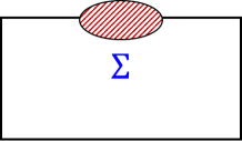
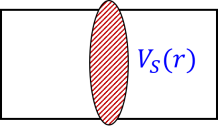
Figure 1: Schematic representations of diagrams contributing to $\Sigma$ and $V_{S}(r)$.

A standard way to confirm cancellation of the $r$-independent IR contributions to $V_{S}(r)$ with the self-energy type contributions is to show cancellation of the $u=1/2$ renormalons in the combination $2m_{\rm pole}+V_{S}(r)$ [31, 32, 33]. By construction of pNRQCD as a low energy EFT, IR contributions to $\Sigma$ and $m_{\rm pole}$ are common. Both $\Sigma$ and $m_{\rm pole}$ are RG invariant, hence ambiguities induced by the leading renormalons both correspond to $u=1/2$ and proportional to $\Lambda_{\overline{\rm MS}}$. This reasoning determines the parameters for the dimensionless potential $rV_{S}(r)$ in eq. (10) and consequently in eq. (6) as

$$\nu_{1/2}=\frac{b_{1}}{2b_{0}^{2}}$$ (27)

and

$$\tilde{c}_{k}=0\quad\text{for $k\geq 1$}\,.$$ (28)

3.3 $u=3/2$ renormalon

To clarify the structure of the $u=3/2$ renormalon, the $r$-dependence of the $u=3/2$ renormalon uncertainty should be revealed (as done in Sec. 2). To this end, we focus on $\delta E_{\rm US}(r)$ [for instance, the expression of eq. (25)], which cancels the corresponding renormalon uncertainty of $V_{S}(r)$. At this stage, we note that computation of $V_{S}(r)$ does not include the US scale, and thus the $u=3/2$ renormalon uncertainty is independent of $\Delta V$. (Supplementary discussion on this point is given in Sec. 3.5.) This reasoning and the expression, for instance, of eq. (25) tell us that the $r$-dependence of the $u=3/2$ renormalon uncertainty is given solely by $\sim r^{2}V_{A}^{2}(r)$. Now we investigate the $r$-dependence of $V_{A}(r)$. Since $V_{A}(r)$ can be renormalized multiplicatively, the RG equation of the form $[\mu^{2}d/(d\mu^{2})-\gamma(\alpha_{s})]V_{A}(r)=0$ follows, where $\gamma(\alpha_{s})=\gamma_{0}\alpha_{s}+\gamma_{1}\alpha_{s}^{2}+\dots$. From this RG equation, the fixed order result of $V_{A}(r)$ takes the form

$$V_{A}(r;\mu)=e_{0}+(e_{1}+e_{0}\gamma_{0}\log(\mu^{2}r^{2}))\alpha_{s}(\mu)+\mathcal{O}(\alpha_{s}^{2})\,.$$ (29)

From the explicit NLO result $V_{A}(r)=1+\mathcal{O}(\alpha_{s}^{2})$ [12], we see that $\gamma_{0}=0$. Thus, we determine the parameter $\nu_{3/2}$ for the dimensionless potential in the Borel transform in eq. (6) as [cf. eq. (16)]

$$\nu_{3/2}=\frac{3b_{1}}{2b_{0}^{2}}\,.$$ (30)

We also clarify that the $u=3/2$ renormalon uncertainty is given by eq. (10) with $(b_{0}\alpha_{s}(1/r))^{-\nu_{u}+ub_{1}/b_{0}^{2}}=1$. The parameters $\tilde{c}_{k}$ can be parametrized by $e_{i}$’s, $\gamma_{i}$’s, and $b_{i}$’s. With the NLO result of $V_{A}$, $\tilde{c}_{1}$ is explicitly obtained as

$$\tilde{c}_{1}=-\gamma_{1}/b_{0}\,.$$ (31)

Thus, a correction factor to the $r$-dependence of the renormalon uncertainty $r^{2}$ is given by $1+\mathcal{O}(\alpha_{s}(1/r))$ with the above $\tilde{c}_{1}$ term. (The explicit result of $\gamma_{1}$ is not known currently.)

3.4 Renormalon in momentum-space potential

We now discuss the renormalon uncertainty in the momentum-space potential. For convenience we define the dimensionless potential as $v(r)=rV_{S}(r)$. Suppose that we have the ambiguity in the position-space potential due to the renormalon at $t=u/b_{0}$ as

$${\rm Im}\,{v}_{\pm}[u]=\pm N_{u}A(u)\,(r^{2}\Lambda_{\overline{\rm MS}}^{2})^{u}\,,$$ (32)

with

$$A(u)=\frac{\pi}{b_{0}}\frac{1}{\Gamma(1+ub_{1}/b_{0}^{2})}u^{1+u\frac{b_{1}}{b_{0}^{2}}}\,.$$ (33)

For $u=1/2$, eq. (32) is exact, whereas the correction factor $1+\mathcal{O}(\alpha_{s}(1/r))$ arises for $u=3/2$. The momentum-space potential is obtained by the Fourier transform of $V_{S}(r)$:

$$\widetilde{V}_{S}(q)=-4\pi C_{F}\frac{\widetilde{\alpha}_{V}(q)}{q^{2}}=\int d^{3}\vec{r}\,e^{-i\vec{q}\cdot\vec{r}}\,V_{S}(r)\,.$$ (34)

Here and hereafter, we denote $\widetilde{V}_{S}(q)$ instead of $\widetilde{V}_{\rm QCD}(q)$ to make explicit that we consider the Fourier transform of the leading Wilson coefficient $V_{S}(r)$, although in naive perturbative expansion $V_{S}(r)$ and ${V}_{\rm QCD}(r)$ coincide; see eq. (24).

From the Fourier transform of $v_{\pm}$, we can obtain the renormalon uncertainty in the $V$-scheme coupling constant in momentum space:

$${\rm Im}\,\widetilde{\alpha}_{V}(q)_{\pm}[u]=\mp\frac{N_{u}}{C_{F}}A(u)\left(\frac{\Lambda_{\overline{\rm MS}}}{q}\right)^{2u}\Gamma(2u+1)\cos({\pi u})\,,$$ (35)

where we have used analytical continuation of the result for $(-1<)u<0$. The above formula shows that, if we assume eq. (32), renormalons of $\widetilde{V}_{S}(q)$ vanish at positive half-integer $u$’s, since $\cos({\pi u})=0$ and $A(u)$ is finite. In particular, the normalization of the renormalon at $u=1/2$ vanishes,

$${\rm Im}\,\widetilde{\alpha}_{V}(q)_{\pm}[u=1/2]=0\,.$$ (36)

For $u=3/2$, while the normalization is not exactly zero, it is suppressed by $\alpha_{s}(q)^{2}$. To see this, one should note first eq. (30) in eq. (10), secondly that $\tilde{c}_{k}$’s are independent of $1/r$ and also $\alpha_{s}(1/r)=\alpha_{s}(q)+b_{0}\log(r^{2}q^{2})\alpha_{s}(q)^{2}+\cdots$. Explicitly, the leading behavior of the $u=3/2$ renormalon uncertainty of $\alpha_{V}(q)$ is given by

$${\rm Im}\,\widetilde{\alpha}_{V}(q)_{\pm}[u=3/2]=\mp\frac{N_{3/2}}{C_{F}}A(u=3/2)\left(\frac{\Lambda_{\overline{\rm MS}}}{q}\right)^{3}\alpha_{s}(q)^{2}\,6\pi b_{0}\tilde{c}_{1}[1+\mathcal{O}(\alpha_{s}(q))]\,,$$ (37)

where $N_{3/2}$ and $\tilde{c}_{1}$ represent the parameters of the position-space potential.

Thus, eqs. (35)–(37) provide a formal framework to analyze renormalons in the momentum-space potential, without recourse to diagrammatic analyses (or resummation of certain diagrams) used in the previous analyses [32, 33, 8].

3.5 Renormalization scheme

So far, we did not specify how to renormalize $V_{S}(r)$ and $\delta E_{\rm US}(r)$, which contain the IR divergences and UV divergences, respectively, Here, we define two schemes to remove the divergences.

Scheme (A)

At each order of the perturbative expansion of ${V}_{S}(r)$ in $\alpha_{s}$, we first set $\mu=1/r$ and then drop all the poles in $\epsilon$ originating from the IR divergences. ($\mu$ denotes the renormalization scale in full QCD. The scale in the argument of the logarithms originating from the IR divergences is also taken as $\mu$, even though it is sometimes distinguished in the literature.) We also redefine $\delta E_{\rm US}$ such that the sum $V_{S}(r)+\delta E_{\rm US}$ is unchanged, which is evaluated in double expansion in $\alpha_{s}$ and $\log\alpha_{s}$. The renormalized $V_{S}$ and $\delta E_{\rm US}$ are both independent of $\mu$ by definition.

In fact, this regularization is compatible with the property used in Sec. 3.3 that $V_{S}(r)$ is RG invariant (see footnote 4), but it may be incompatible with the one that the $r$-dependence of the $u=3/2$ renormalon uncertainty is given by $\sim r^{2}V^{2}_{A}(r)$. This is because the latter reasoning [and thus the results such as eq. (30)] relies on eq. (25) and additional contribution was not considered. However, we assume that the structure of IR renormalons in $V_{S}(r)$ at ${\cal O}(r^{2})$ is unchanged by this prescription. This is indeed the case in the large-$\beta_{0}$ approximation of $\delta E_{\rm US}$, in which the IR divergences and IR renormalons are clearly separated; the former is given as a convergent series in $\alpha_{s}$ expansion, while the latter is given as a factorially diverging series. This is shown by computing $\delta E_{\rm US}$ in the large-$\beta_{0}$ approximation [41]:

$$\delta E_{\rm US}(r)\Bigr{|}_{\text{large-$\beta_{0}$}} = \frac{C_{F}\alpha_{s}}{4\pi}\,8r^{2}\,\Delta V(r)^{3}\sum_{n=0}^{\infty}\left({b_{0}\alpha_{s}}\right)^{n}\left[n!\,G_{n+1}+\frac{1}{\epsilon^{n+1}}\,\frac{(-1)^{n}}{n+1}\,g(\epsilon)\right]$$ (38)

$$+\,{\cal O}(\epsilon,r^{3})$$

where

$$G(u)\equiv\sum_{j=0}^{\infty}G_{j}u^{j}=\left[\frac{\mu_{f}\,e^{5/6}}{2\,\Delta V(r)}\right]^{2u}\,\frac{2\,\Gamma(2-u)\,\Gamma(2u-3)}{\Gamma(u-1)}\,,$$ (39)

$$g(\epsilon)=\frac{\Gamma(4-2\epsilon)}{36\,\Gamma(1+\epsilon)\,\Gamma(2-\epsilon)^{2}\,\Gamma(1-\epsilon)}\,.$$ (40)

The UV divergences and UV renormalons of $\delta E_{\rm US}(r)$ are canceled, respectively, by the IR divergences and IR renormalons of $V_{S}(r)$. In addition, the US logarithms at LL [12] and NLL [13, 42], associated with the IR divergences in $V_{S}(r)$, are known to be given by convergent series in $\alpha_{s}$ expansion, computed explicitly using the RG equation of pNRQCD. Thus, to the best of our knowledge, the above assumption seems to be valid. As a result, we consider that the scheme (A) is suitable for studying the renormalon of $V_{S}(r)$, where the renormalon structure revealed in Sec. 3.3–3.4 based on the OPE is not expected to be modified.

We note the existence of the UV renormalons at $u=3/2$, $1/2$, $-1/2$, $-3/2$, $\cdots$ of $\delta E_{\rm US}$ in eq. (39). It is confirmed that the leading UV renormalon at $u=3/2$ cancels the known ${\cal O}(r^{2})$ IR renormalon of $V_{S}(r)$ in the large-$\beta_{0}$ approximation [41, 43]. The subleading renormalon at $u=1/2$ is also expected to be canceled against $V_{S}(r)$ (although it cannot be confirmed within the large-$\beta_{0}$ approximation) since the IR structure of $V_{S}(r)$ should match the UV structure of $\delta E_{\rm US}$. The residues of the subleading renormalons at smaller $u$ are proportional to higher powers of $\Delta V(r)/\mu_{f}$. This leads to less powers of $r$, which contradicts to the naive expectation that the renormalons of $V_{S}(r)$ beyond $u=3/2$ are suppressed by higher powers of $r$ in accordance with the multipole expansion. This feature originates from the fact that if we expand the integrand of eq. (25) in $\Delta V$, higher power singular IR behaviors $\sim(\Delta V(r)/k)^{n}$ appear. [Note that $\langle\,{E}^{a}_{i}\,\varphi_{\rm adj}^{ab}\,{E}^{b}_{j}\,\rangle(k)$ is independent of $\Delta V$.] The IR structure of $V_{S}(r)$ includes the same power behaviors, since the IR structure of $\delta E_{\rm US}$ is common to that of $V_{S}(r)$ once the integrand is expanded in $\alpha_{s}$. The higher power singular IR behaviors generate the above more singular IR renormalons as well as higher power IR divergences.

The above observation in particular means that $V_{S}(r)$ has a renormalon at $u=1/2$ corresponding to the above UV renormalon of $\delta E_{\rm US}$. The $u=1/2$ renormalon uncertainty is given by $\mathcal{O}(\Lambda_{\overline{\rm MS}}r^{2}\Delta V(r)^{2})$, as seen from eqs. (38) and (39). It is similar to the form which is derived by the RG equations of the US scale $\mu_{f}$ on the assumption that $\mathcal{O}(r^{0})$ terms (up to anomalous dimensions) are contained in $V_{S}(r)$ [13]. In particular, a $\mu_{f}$-independent term $\sim\Lambda_{\overline{\rm MS}}r^{2}\Delta V(r)^{2}$, which is of the same form as the renormalon uncertainty, can be added to Eq. (25) in Ref. [13] without spoiling the solution to the RG equations (or we can say that this term is included in the $\mu_{f}$-independent but possibly $r$-dependent constant $\Lambda$ in this equation). This renormalon is different from the familiar renormalon at $u=1/2$, which induces an $r$-independent uncertainty. (See footnote 8.) We note that this unfamiliar renormalon at $u=1/2$ can be an obstacle in estimating the normalization constants of the familiar renormalons at $u=1/2$ and $3/2$. This possibility is taken into account later in numerical analyses, while we also present naive analysis by simply neglecting this peculiar renormalon.

We make comments on the $\Delta V$-dependence of $V_{S}(r)$. As already mentioned, perturbative computations of $V_{S}(r)$ do not include $\Delta V$ as an external scale. However, $\Delta V$ appears (only) in an implicit way in a form $\alpha_{s}\times(\text{soft scale})$. Hence, the above renormalon uncertainty of $\mathcal{O}(\Lambda_{\overline{\rm MS}}r^{2}\Delta V^{2})$ in $\delta E_{\rm US}$ corresponds to the renormalon uncertainty in $V_{S}(r)$ of $\mathcal{O}(\Lambda_{\overline{\rm MS}}\alpha_{s}(1/r)^{2})$, where $\Delta V$ is expanded in $\alpha_{s}$.

One might then wonder if such implicit $\Delta V$-dependence ruins the argument in Sec. 3.3 that the $u=3/2$ renormalon uncertainty of $V_{S}(r)$ is independent of $\Delta V$. In fact this argument is correct for the $u=3/2$ renormalon; the $u=3/2$ renormalon of $V_{S}(r)$ is canceled against the leading UV contribution of $\delta E_{\rm US}$, where $\Delta V$ in Eq. (25) is not relevant.

Scheme (B)

We subtract IR divergences from $V_{S}(r)$ by adding $\delta E_{\rm US}$ evaluated in double expansion in $\alpha_{s}$ and $\log\alpha_{s}$ (Scheme B1). In this scheme, we do not distinguish $V_{S}(r)$ and $\delta E_{\rm US}$, and we exclusively treat the sum of them, which is regarded as a redefined $V_{S}(r)$. In this way we can subtract the IR divergences. Furthermore, after canceling the IR divergences, we can replace the argument of US logarithms as $\log(r\Delta V)\to\log(r\mu_{f})$ (Scheme B2). Since both ${V}_{\rm QCD}(r)$ and $\Delta V(r)$ are $\mu$ independent, the renormalized $V_{S}(r)$’s are also $\mu$ independent up to ${\cal O}(r^{2})$ (although $V_{S}^{\rm(B2)}(r)$ is $\mu_{f}$ dependent).

Finally we point out that it is not straightforward to cancel simultaneously both the IR divergences and IR renormalon at $u=3/2$ of $V_{S}$ in the sum $V_{S}+\delta E_{\rm US}$. We can observe this in the large-$\beta_{0}$ approximation. The renormalon uncertainty of $\delta E_{\rm US}$ coincides with minus that of $V_{S}(r)$ when $\Delta V$ in $\delta E_{\rm US}$ is not expanded in $\alpha_{s}$. If $\Delta V$ is perturbatively expanded instead, the power of $\alpha_{s}$ shifts by three in the perturbative series due to $\Delta V=\mathcal{O}(\alpha_{s})$, as seen from eq. (38), and the renormalon cancellation breaks down. Hence, it would be optimal not to expand $\Delta V$ in $\alpha_{s}$ for the renormalon cancellation. On the other hand, this prescription is not preferable to cancel the IR divergences. The IR divergences are cancelled when $\Delta V$ is expanded in $\alpha_{s}$ as the IR and UV divergences in $V_{S}$ and $\delta E_{\rm US}$, respectively, appear at $\mathcal{O}(\alpha_{s}^{4})$. The proposed two schemes above can remove the IR divergences from $V_{S}(r)$, but cannot remove the IR renormalons of $V_{S}(r)$. It remains a future task to develop a method for subtracting the IR renormalons completely.

3.6 Renormalon subtraction by contour deformation

One motivation of the above investigation is to give a justification to the method used to subtract the $u=1/2$ and $3/2$ renormalons from ${V}_{\rm QCD}(r)$ in a recent determination of $\alpha_{s}(M_{Z})$ [29]. There, it is assumed that the corresponding renormalons contained in $\widetilde{V}_{S}(q)$ can be neglected. (The IR divergences are canceled in momentum space.) Then, using the one parameter integral form with respect to the momentum $q$ and deforming the integral contour in the complex $q$-plane, the renormalons at $u=1/2$ and $3/2$ which stem from the original $q$ integral are subtracted. See Refs. [48, 29] for the details. As we have seen above, the normalization of the $u=1/2$ renormalon in the momentum-space potential is exactly zero, while the $u=3/2$ renormalon is suppressed by $\alpha_{s}(q)^{2}$. While the $r^{2}\Lambda_{\overline{\rm MS}}^{3}$ renormalon that is generated purely by the $q$ integral is subtracted, the suppressed renormalon in $\tilde{\alpha}_{V}(q)$ can still contribute to the position-space potential. That is, if $\tilde{\alpha}_{V}(q)$ exhibits renormalon divergence, its uncertainty will give an uncertainty to the renormalon-subtracted $V_{S}(r)$ constructed by the contour deformation method. It is expected to generate a renormalon of order $r^{2}\Lambda_{\overline{\rm MS}}^{3}\alpha_{s}(1/r)$ in the renormalon-subtracted $V_{S}(r)$, corresponding to the correction proportional to $\tilde{c}_{1}$ of Sec. 3.3.

4 Numerical study of $u=1/2$ renormalon

In the rest of this paper we perform numerical analyses on the normalizations $N_{u}$ of renormalons to check the above observations and to see the current status of our knowledge on the perturbative series for $V_{S}(r)$ and $\widetilde{V}_{S}(q)$. We treat two perturbative series: one is the fixed order perturbative series, and the second one includes higher-order terms estimated by RG, which is used extensively in Refs. [47, 48].

In the case that the renormalon singularity of the Borel transform is given by eq. (6), we can estimate the normalization constant $N_{u}$ from the fixed-order result of the perturbative series. This was first proposed in Ref. [36], whose method is as follows. We consider the function

$$N(t)=\left(1-\frac{b_{0}t}{u}\right)^{1+\nu_{u}}B_{X}(t;\mu=Q)\,.$$ (42)

(In the following analyses, $\nu_{u}$ of eqs. (27) and (30) are used.) We can obtain the normalization constant by expanding this function in $t$ and then substituting $t=u/b_{0}$:

$$N_{u}=\sum_{i=0}^{\infty}N_{i}t^{i}|_{t=u/b_{0}}\,,$$ (43)

as long as the corresponding renormalon is the closest one to the origin. This method is fairly general and can be used with only known terms of the perturbative series.

Using this method, Ref. [37] first studied $N_{1/2}$ from the fixed-order result. In Ref. [18], $N_{1/2}$ is estimated with a more recent NNNLO result [15, 16]. We present the NNNLO result [17] by subtracting the IR divergence at NNNLO in the scheme (A),

$$N_{1/2} =-1.3333\quad\text{at LO}$$

$$=-0.76139\quad\text{at NLO}$$

$$=-1.10661\quad\text{at NNLO}$$

$$=-1.21655\quad\text{at NNNLO}\,.$$ (44)

[If we adopt the scheme (B2), the NNNLO result is given by $N_{1/2}=-1.07764-0.0541542\log(2r\mu_{f})$.] We note that the IR logarithm in the NNNLO perturbative coefficient considered here is different from Ref. [18]. We adopt the result in dimensional regularization given in ref. [15] (more precisely its Fourier transform), while ref. [18] adopted the result in Ref. [8]. (As a result, the IR logarithms differ by factor $4$.) This difference corresponds to different choices of renormalization scheme.

We also examine the scale dependence of the estimated normalization constant. We use the perturbative coefficients with the renormalization scale $\mu=s/r$ to estimate the normalization constant. The results are shown in Fig. 2.

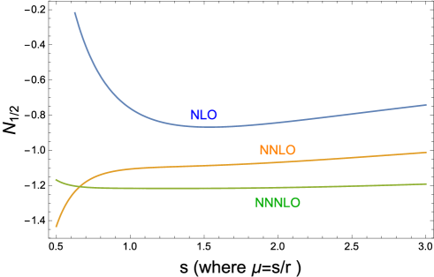
Figure 2: Scale dependence of the normalization constant $N_{1/2}$.

The scale dependence decreases as we include higher-order terms. These results indicate that the series (43) shows convergence for the $u=1/2$ renormalon and $N_{1/2}(s=1)\simeq-1.1$.

In the second method we treat the RG-improved series, where the higher-order terms in perturbative series are estimated by RG. Explicitly we can use [47, 48]

$$v(r)=-\frac{2C_{F}}{\pi}\int_{0}^{\infty}\frac{dq}{q}\,\sin(qr)[\widetilde{\alpha}_{V}(q)]_{\text{N${}^{k}$LL}}\,,$$ (45)

where the N^kLL terms of the perturbative series [coefficients of $\alpha_{s}(\mu)^{n+k+1}\,\log^{n}(\mu r)$ for arbitrary $n$] can be determined using the $(k+1)$-loop beta function and the fixed-order result up to $k$-loops.

We now estimate $N_{1/2}$ from the RG-improved series obtained from eq. (45) using eq. (43). Since we have an all-order perturbative series (at each order of improvement), we can obtain $N_{\rm LL},\cdots,N_{\rm N^{3}LL}$ with arbitrary precision in principle. The results from finite number of terms read

$$N_{1/2} =-0.8488\quad\text{at LL (using 30 terms)}$$

$$=-0.7603\quad\text{at NLL (using 30 terms)}$$

$$=-1.009\quad\text{at NNLL (using 30 terms)}$$

$$=-1.120\quad\text{at NNNLL (using 30 terms)}\,.$$ (46)

We use the scheme (A) to subtract the IR divergence in the NNNLL analysis. From Table 1, which shows the convergence speed, we infer that 20-50 perturbative coefficients are needed in order to obtain the normalization constants with one-percent accuracy.

The number of terms	LL	NLL	NNLL	NNNLL
1	$-1.33333$	$-1.33333$	$-1.33333$	$-1.33333$
2	$-0.769621$	$-0.761390$	$-0.761390$	$-0.761390$
3	$-0.770430$	$-0.553531$	$-1.10661$	$-1.10661$
4	$-0.893478$	$-0.764315$	$-0.893382$	$-1.21655$
5	$-0.834305$	$-0.777275$	$-0.973020$	$-1.03927$
10	$-0.848814$	$-0.758382$	$-1.00381$	$-1.11924$
15	$-0.848826$	$-0.759417$	$-1.00658$	$-1.11968$
20	$-0.848826$	$-0.759892$	$-1.00779$	$-1.11995$
25	$-0.848826$	$-0.760151$	$-1.00844$	$-1.12010$

Table 1: Estimates of normalization constant $N_{1/2}$ from truncated perturbative series of the RG-improved series.

5 Renormalon cancellation in total energy

It is interesting to examine renormalon cancellation in the total energy (namely, $V(r)+2m_{\rm pole}$) from the estimated $N_{1/2}$ [37]. The leading renormalon in the Borel transform of $m_{\rm pole}/m_{\rm{\overline{MS}}}$ is given by

$$B_{m_{\rm pole}/m_{\overline{\rm MS}}}(\mu=m_{\overline{\rm MS}})\simeq\frac{N_{M}}{(1-2b_{0}t)^{1+\frac{b_{1}}{2b_{0}^{2}}}}\,.$$ (47)

$N_{M}$ can be investigated from the fixed-order perturbative series [49, 50] in a parallel manner. The results of $N_{M}$ are given by ($\mu=m_{\rm{\overline{MS}}}$)

$$N_{M} =0.424413\quad\text{at LO}$$

$$=0.562265\quad\text{at NLO}$$

$$=0.574979\quad\text{at NNLO}$$

$$=0.513427\pm 0.001025\quad\text{at NNNLO}\,.$$ (48)

The last result has an error due to the numerical error of the $\mathcal{O}(\alpha_{s}^{4})$ coefficient. Now let us examine the renormalon cancellation, $2N_{M}+N_{1/2}=0$.

$$\frac{2N_{M}+N_{1/2}}{(2N_{M}-N_{1/2})/2} =-0.444\quad\text{at LO}$$

$$=0.385\quad\text{at NLO}$$

$$=0.038\quad{\text{at NNLO}}$$

$$=-0.088\pm 0.002\quad{\text{at NNNLO}}$$ (49)

It is possible that treatment of IR divergences affects the cancellation. Let us examine this. So far, we subtracted the IR divergence in the scheme (A), but now we make the three-loop coefficient finite in the scheme (B2). Then, the IR divergence is replaced by the logarithmic term like $\log(\mu_{f}r)$. In Fig. 3, we investigate renormalon cancellation while varying $\mu_{f}$ in this logarithm in a reasonable range. This figure shows that the treatment of IR divergences can be non-negligible to the precise cancellation. We note that the numerical error on the four-loop result of the mass relation hardly affects this result.

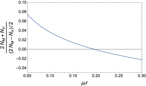
Figure 3: Renormalon cancellation as a function of $\mu_{f}$ in the logarithm.

6 Normalization by analytic formula in RG-improved series

For the RG-improved series, we derive a formula for the normalization constants of renormalons given as a one-dimensional integral. The Borel integral of the QCD potential for the RG-improved series can be written as

$$\,{v}_{\pm}=-\frac{2C_{F}}{\pi}\int_{C_{\mp}}\frac{dq}{q}\,\sin(qr)[\widetilde{\alpha}_{V}(q)]_{\text{N${}^{k}$LL}}\,,$$ (50)

where the contours $C_{\mp}$ are displayed in Fig. 4. The details of the derivation are given in App. B. Since the integrand satisfies $\{f(x)\}^{*}=f(x^{*})$, the imaginary part can be calculated by a contour integral

$${\rm Im}\,{v}_{\pm}=\mp\frac{2C_{F}}{\pi}\frac{1}{2i}\int_{C}\frac{dq}{q}\sin(qr)\widetilde{\alpha}_{V}(q)\,,$$ (51)

where the contour $C$ is displayed in Fig. 4.

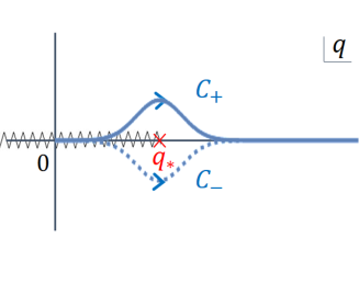
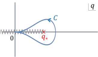
Figure 4: Contours $C_{\pm}$ and $C$. $q_{*}$ is the singular point of $\widetilde{\alpha}_{V}(q)$ on the positive real $q$ axis.

By expanding $\sin(qr)$ in $qr$, the normalization of the renormalon at $u=1/2$ is found as

$${\rm Im}\,{v}_{\pm}[{\textstyle u=\frac{1}{2}}] =\mp\frac{2C_{F}}{\pi}\frac{1}{2i}r\int_{C}dq\,\widetilde{\alpha}_{V}(q)$$

$$=\mp\frac{2C_{F}}{\pi}\Lambda_{\overline{\rm MS}}r\frac{1}{2i}\int_{C}dx\,\widetilde{\alpha}_{V}(x)\,.$$ (52)

In the last line, we changed the integration variable to $x=q/\Lambda_{\overline{\rm MS}}$. (Note that $\widetilde{\alpha}_{V}(q)$ is a function of $q/\Lambda_{\overline{\rm MS}}$.) Then, from eqs. (10) and (52), we obtain

$$N_{1/2}=-\frac{2C_{F}}{\pi}\frac{b_{0}}{\pi}\Gamma(1+ub_{1}/b_{0}^{2})u^{-1-u\frac{b_{1}}{b_{0}^{2}}}I_{u}|_{u=1/2}\,,$$ (53)

with

$$I_{1/2}=\frac{1}{2i}\int_{C}dx\,\widetilde{\alpha}_{V}(x)\,.$$ (54)

We present numerical values of $N_{1/2}$ via numerical evaluation of $I_{1/2}$:

$$N_{1/2} =-0.848826\quad\text{at LL}$$

$$=-0.760846\quad\text{at NLL}$$

$$=-1.01017\quad\text{at NNLL}$$

$$=-1.12049\quad\text{at NNNLL}\,.$$ (55)

They agree well with the estimates from the finite number of terms (46). The scheme (A) is adopted at NNNLL in accordance with Sec. 4.

It is possible to calculate the normalization constants of other renormalons in a parallel manner. The normalization constant of a general renormalon at $u$ is expressed as

$$N_{u}=-\frac{2C_{F}}{\pi}\frac{b_{0}}{\pi}\Gamma(1+ub_{1}/b_{0}^{2})u^{-1-u\frac{b_{1}}{b_{0}^{2}}}I_{u}$$ (56)

with

$$I_{u}=\frac{1}{2i}\int_{C}dx\,\frac{(-1)^{(2u-1)/2}}{(2u)!}x^{2u-1}\widetilde{\alpha}_{V}(x)\,.$$ (57)

This expression stems from the Taylor expansion of $\sin(qr)$.

In this method, the $r$-dependence of a renormalon uncertainty due to any half-integer renormalon at $u$ is given exactly by $r^{2u+1}$. In particular for $u=3/2$, the correction factor of $[1+\mathcal{O}(\alpha_{s}(1/r))]$ is not detected (as long as we work at N^kLL with finite $k$). It is because this method relies on the assumption that $\alpha_{V}(q)$ does not possess renormalon uncertainties.

For the $u=3/2$ renormalon, which is the second IR renormalon, the numerical values of $N_{3/2}$ are given by

$$N_{3/2} =0.0471570\quad\text{at LL}$$

$$=0.0260142\quad\text{at NLL}$$

$$=0.0793089\quad\text{at NNLL}$$

$$=0.143286\quad\text{at NNNLL}\,,$$ (58)

based on eqs. (56) and (57). We again adopt the scheme (A).

7 Numerical analysis of $u=3/2$ renormalon

We now estimate $N_{3/2}$ from the fixed-order result. We annihilate the leading renormalon at $u=1/2$, whose uncertainty is an $r$-independent constant, by considering the QCD force. Then we use the same method as in the $u=1/2$ renormalon.

We first examine the relation between the normalization constants of the potential and force. The potential $v=rV$ has the $u=3/2$ renormalon uncertainty as eq. (10) with eqs. (30) and (31), which gives the uncertainty to the dimensionless force $f=r^{2}dV/dr$ as

$${\rm Im}\,{f}_{\pm}=\pm\frac{\pi}{b_{0}}\frac{2N_{3/2}}{\Gamma(1+ub_{1}/b_{0}^{2})}u^{1+u\frac{b_{1}}{b_{0}^{2}}}(r^{2}\Lambda_{\overline{\rm MS}}^{2})^{3/2}[1+\mathcal{O}(\alpha_{s}(1/r))]|_{u=3/2}\,.$$ (59)

Thus, the normalization constant of the dimensionless force $N_{3/2}^{F}$ is related as $N_{3/2}=\frac{1}{2}N_{3/2}^{F}$.

To obtain $N_{3/2}$, we first consider the fixed-order perturbative series of the potential without setting $\mu=1/r$. The derivative with respect to $r$ gives the fixed-order result of the force. Finally we set $\mu=1/r$ to estimate $N_{3/2}^{F}$ and translate it to $N_{3/2}$.

We present the results:

$$N_{3/2} =0.666667\quad\text{at LO}$$

$$=-0.857914\quad\text{at NLO}$$

$$=1.15844\quad\text{at NNLO}$$

$$=1.02659\quad\text{at NNNLO}\,.$$ (60)

We adopt the scheme (A) to obtain the NNNLO result. [In the scheme (B2), we obtain $N_{3/2}=-0.848623+0.731082\log(2\mu_{f}r)$ at NNNLO.] Although the estimate of the normalization constant may look already convergent, this seems to be a numerical accident. We examine the scale dependence of the estimated normalization constant in a parallel manner to the $u=1/2$ renormalon. The result is shown in Fig. 5. We find that large dependence on the renormalization scale remains in this estimate.

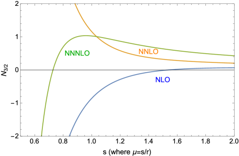
Figure 5: Scale dependence of the normalization constant $N_{3/2}$.

Let us perform a parallel estimate from the finite order result of the RG-improved series. In this case, since we know $N_{3/2}$ as given by eq. (58), it would be useful to grasp how many terms are needed for a reasonable estimate. Table 2 shows the result. At NNNLL, we adopt the scheme (A). One sees that typically 20 terms are needed for a good estimate.

The number of terms	LL	NLL	NNLL	NNNLL
1	$0.666667$	$0.666667$	$0.666667$	$0.666667$
2	$-0.845569$	$-0.857914$	$-0.857914$	$-0.857914$
3	$0.00364088$	$-1.33043$	$1.15844$	$1.15844$
4	$1.66115$	$3.05043$	$-3.33613$	$1.02659$
5	$-2.39650$	$0.00590101$	$3.26898$	$-7.65424$
10	$-0.525249$	$1.23022$	$-1.32332$	$-5.59838$
15	$0.0300462$	$-0.00224226$	$0.1238239$	$0.294562$
20	$0.0471086$	$0.0254835$	$0.0802829$	$0.151007$
25	$0.0471576$	$0.0260084$	$0.0791596$	$0.143535$
30	$0.0471570$	$0.0260113$	$0.0792097$	$0.143424$

Table 2: Estimates of the normalization constant $N_{3/2}$ from truncated perturbative series of the RG-improved series.

We examine scale dependence of the estimate of $N_{3/2}$ using finite number of terms in the RG-improved series. Since we know the exact answer in this case, we can directly check whether mild scale dependence indicates reliability of the estimate. In Fig. 6, we examine this at NNLL.

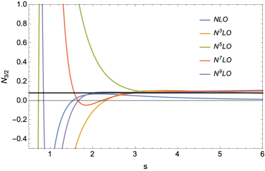
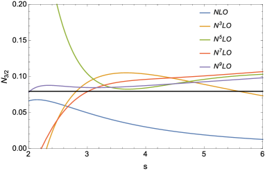
Figure 6: Scale dependence of $N_{3/2}$ determined from finite number of terms at NNLL. Black line shows the exact answer obtained from the analytic formula. In the right panel, the range $2\leq s\leq 6$ is magnified.

We see that at higher order the scale dependence of $N_{3/2}$ decreases and it approaches the correct value. (At further higher order, for instance from 30 terms, we obtain $N_{3/2}=0.0079136$ and $0.079172$ for $s=1/2$ and $2$, respectively.)

In Sec. 3.5, we pointed out that $V_{S}(r)$ can have the unfamiliar renormalon at $u=1/2$ associated with the IR divergences. Since the corresponding renormalon uncertainty for the static QCD potential is not an $r$-independent constant in contrast to the familiar renormalon at $u=1/2$, this renormalon cannot be eliminated in the QCD force. Taking into account this possibility, we present another estimate for the $u=3/2$ renormalon, whose method is not plagued by the two renormalons at $u=1/2$. We carry out this by using a mapping from the $t$-plane to a new $z$-plane, where the $u=3/2$ renormalon becomes closer to the origin than the $u=1/2$ renormalon. Namely we change the relative distances of the two IR renormalons from the origin.

A possible mapping is given by

$$b_{0}t(z)=\frac{1}{2}(z+e^{i\pi/6})^{6}+\frac{1}{2}\,.$$ (61)

The basic idea to obtain this mapping is as follows. In the first step, we consider $v=2(b_{0}t)-1$, which maps $b_{0}t=0$, $1/2$, $3/2$ into $v=-1$, $0$, $2$, respectively. In the second step, $w=v^{1/6}$ is considered, which makes the distance between $v=-1$ $(u=0)$ and $v=2$ $(u=3/2)$ shorter than that between $v=-1(u=0)$ and $v=0(u=1/2)$. The final step is given by $z=v-e^{i\pi/6}$ to locate the original origin $u=0$ at $z=0$. Corresponding to these transformations, we consider Eq. (61). Indeed, the closest zero of $1-b_{0}t(z)/u$ among positive half-integers $u$ is given by $u=3/2$.

However, it turned out that with the above mapping convergence is too slow for practical analysis. (e.g., In RG-improved series at LL, we need 250 terms to obtain the normalization constant with about 10 % accuracy.) Instead of Eq. (61), we use

$$b_{0}t(z)=2-\frac{1}{2}[9-7(e^{i\pi/6}-z)^{6}]^{1/2}\,.$$ (62)

This mapping is obtained with a similar idea to the above, but the main difference is that we first consider square of the difference from $b_{0}t=2$, i.e. $(2-b_{0}t)^{2}$. The mapping (62) consists of the following steps: $b_{0}t(v)=2-v^{1/2}$, $v(w)=-\frac{7}{4}w+\frac{9}{4}$, $w(y)=y^{6}$, $y(z)=-z+e^{i\pi/6}$. We note that the singularities of $1/(1-2b_{0}t(z)/3)$ and $1/(1-2b_{0}t(z)/5)$ with respect to $z$ are not common, and the $u=5/2$ renormalon does not affect the estimate of the normalization constant at $u=3/2$. With this mapping $t(z)$, we consider a function

$$N(z)=\left(1-\frac{2}{3}b_{0}t(z)\right)^{1+\frac{3}{2}\frac{b_{1}}{b_{0}^{2}}}B_{v}(t(z);\mu=1/r)\,.$$ (63)

By expanding this function in $z$ and then substituting $z=-(8/7)^{1/6}+e^{i\pi/6}$, we can obtain the normalization constant of the $u=3/2$ renormalon.

Using this mapping, we estimate the normalization constant of the $u=3/2$ renormalon from the fixed-order perturbative series as

$$N_{3/2} =-1.33333\quad\text{at LO}$$

$$=-1.52383\quad\text{at NLO}$$

$$=4.75182\quad\text{at NNLO}$$

$$=9.01375\quad\text{at NNNLO}\,.$$ (64)

We adopt the scheme (A) at NNNLO. [In the scheme (B2), we obtain $N_{3/2}=7.2395+0.69179\log(2\mu_{f}r)$.] In this method, imaginary parts appear in fixed-order results, but we omit them in the above estimate since we know that the true normalization is real. The size of the imaginary parts can be used for an error estimate of the results.

We also estimate $N_{3/2}$ of the RG-improved series using this mapping. Table 3 shows the result. One can confirm that the estimated values converge to the results in Eq. (58). We start to obtain reasonable results with about 60 terms.

The number of terms	LL	NLL	NNLL	NNNLL
1	$-1.33333$	$-1.33333$	$-1.33333$	$-1.33333$
2	$-1.52878$	$-1.52383$	$-1.52383$	$-1.52383$
3	$1.20631$	$0.96708$	$4.75182$	$4.75182$
4	$4.86579$	$6.76949$	$4.88592$	$9.01375$
5	$6.13184$	$6.39316$	$-9.64487$	$8.39204$
10	$-1.32119$	$30.9456$	$-220.002$	$277.649$
20	$-12.5409$	$20.1377$	$75.0878$	$-347.457$
30	$4.04035$	$-14.7808$	$66.2768$	$-32.0964$
40	$-1.07937$	$0.943337$	$-5.54367$	$-70.4336$
50	$0.0725315$	$0.0420682$	$0.0878506$	$2.16533$
60	$0.047093$	$0.0258843$	$0.078969$	$0.167635$
100	$0.0471979$	$0.0262156$	$0.0801885$	$0.143394$
150	$0.0471763$	$0.0260685$	$0.0794704$	$0.143429$
200	$0.0471475$	$0.0259836$	$0.0792261$	$0.143089$

Table 3: Estimates of the normalization constant $N_{3/2}$ with using mapping (62) from truncated perturbative series of the RG-improved series.

8 $u=1/2$ and $3/2$ renormalons in $\widetilde{V}_{S}(q)$

Let us investigate the renormalon uncertainty of $\widetilde{\alpha}_{V}(q)$. We estimate the normalization constants of the renormalons of $\widetilde{\alpha}_{V}(q)$ at $u=1/2$ and $3/2$ assuming that they are the leading renormalon individually. More explicitly we assume

$$B_{\widetilde{\alpha}_{V}(q)}(t)\simeq\frac{N_{\widetilde{\alpha}_{V},u}}{(1-\frac{b_{0}}{u}t)^{1+u\frac{b_{1}}{b_{0}^{2}}}}\,.$$ (65)

The theoretical discussion in Sec. 3.4 shows that the normalization constants $N_{\widetilde{\alpha}_{V},u}$ defined in this way should be zero both for $u=1/2$ and $u=3/2$, because the $u=1/2$ renormalon is completely absent in $\tilde{\alpha}_{V}(q)$, and for $u=3/2$ the expansion of the Borel transform around the singularity takes a form $\sim(1-b_{0}t/u)^{-1-ub_{1}/b_{0}^{2}+2}$ rather than $\sim(1-ub_{0}t/u)^{-1-ub_{1}/b_{0}^{2}}$ corresponding to the $\alpha_{s}(q)^{2}$ suppression.

The estimates from the fixed-order results read

$$N_{\widetilde{\alpha}_{V},u=1/2} =1\quad\text{at LO}$$

$$=-0.00617284\quad\text{ at NLO}$$

$$=0.141682\quad\text{at NNLO}$$

$$=-0.0318992\quad\text{at NNNLO}$$ (66)

and

$$N_{\widetilde{\alpha}_{V},u=3/2} =1\quad\text{at LO}$$

$$=-0.0185185\quad\text{at NLO}$$

$$=2.246032\quad\text{at NNLO}$$

$$=2.27727\quad\text{at NNNLO}\,.$$ (67)

We subtract the IR divergence at NNNLO in the scheme (A). If we instead use the scheme (B2), the NNNLO results are modified as

$$N_{\widetilde{\alpha}_{V},u=1/2}=-0.136078+0.0406157\log({2r\mu_{f}})\quad\text{at NNNLO}\,,$$ (68)

and

$$N_{\widetilde{\alpha}_{V},u=3/2}=-0.535547+1.09662\log({2r\mu_{f}})\quad\text{at NNNLO}\,.$$ (69)

By taking $r\mu_{f}=0.2$ as an example, we obtain $N_{\widetilde{\alpha}_{V},u=1/2}=-0.1723293$ and $N_{\widetilde{\alpha}_{V},u=3/2}=-1.54037$ at NNNLO.

In Fig. 7 we show the estimates of $N_{\widetilde{\alpha}_{V},u=1/2}$ and $N_{\widetilde{\alpha}_{V},u=3/2}$ from the RG-improved series, in addition to the ones from the fixed order results. In these figures, we subtract the IR divergence in the scheme (A) at NNNLO. (Note that in the RG-improved series the terms beyond N³LO are zero for $\widetilde{V}_{S}(q)$ since we set $\mu=q$.) We also plot their estimates using the large-$\beta_{0}$ approximation for the higher-order terms (they are non-zero even beyond N³LO). In both cases we know that the normalization constants are zero. We see in the figures that the estimates approach zero as we include more terms. Since the normalization constants are expected to be zero (even if we do not use any approximation), this figure shows overall consistency.

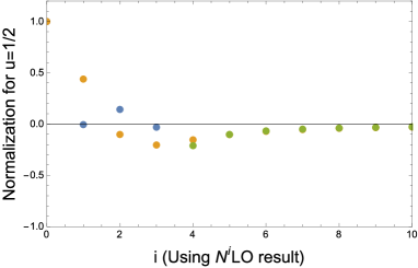
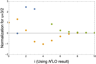
Figure 7: Estimates of the normalization constants of the renormalons at $u=1/2$ (left) and $3/2$ (right) for the momentum-space potential. Green points are obtained from the RG-improved series, while the orange points correspond to the large-$\beta_{0}$ approximation. The first four points of the RG-improved series coincide with the exact fixed-order results, shown by blue points. In the right panel the $i=4$ point ($-7.30$) lies out of the plot range.

Thus, in both cases the observed results are consistent with the expectation that the renormalon at $u=1/2$ is absent and the $u=3/2$ renormalon is suppressed. For $u=1/2$, we may already observe smallness of the renormalon contribution from the known perturbative series. For $u=3/2$, however, the number of terms are much too few to make any statement on the size of the renormalon. By using the formula (35) and the fact that $r$-dependence of $V_{A}=1+{\cal O}(\alpha_{s}^{2})$ is suppressed, we can make a stronger prediction on the smallness of the renormalon. We confirm validity of this formula using the higher-order estimates by RG-improvement (trivial) or by the large-$\beta_{0}$ approximation.

9 Conclusions

We have investigated the $u=1/2$ and $u=3/2$ renormalons in the static QCD potential in position space and momentum space. In particular we have presented detailed examinations of the $u=3/2$ renormalon for the first time. In terms of pNRQCD EFT, we have studied the renormalon of the Wilson coefficient $V_{S}(r)$ (and in connection with this the second term of the multipole expansion, $\delta E_{\rm US}$, as well).

We have determined the structure of the $u=3/2$ renormalon based on the OPE (or multipole expansion) and the RG equations. Although there are non-trivial features specific to the QCD potential (originating from the fact that the multi-scales are involved), we find that the renormalon uncertainty can be parameterized (besides the overall normalization) similarly to the general case as reviewed in Sec. 2. The relevant parameters are the Wilson coefficient of the $\mathcal{O}(\vec{r})$ interaction $V_{A}$, in particular its anomalous dimension (associated with the logs from the soft scale), and also the coefficients of the beta function. We have also clarified how the renormalon uncertainties of the position-space potential propagate to the momentum-space potential. The $u=1/2$ renormalon is completely absent in the momentum-space potential, and the $u=3/2$ renormalon uncertainty is suppressed by $\alpha_{s}(q)^{2}$ in momentum space compared to that in position space. While the renormalon uncertainty of the momentum-space potential has been believed to be small, our result provides a quantitative insight on this issue. We have given a systematic and precise analysis of the old problem, including renormalization prescription and treatment of the IR divergences (US logarithms) based on the multipole expansion in the pNRQCD EFT.

There are some difficulties caused by the IR divergences, however. First, it is not obvious whether the renormalization of $V_{S}(r)$ to remove the IR divergences affects the renormalon structure detected from the OPE argument. We have proposed a way to remove the IR divergences which is likely to keep the renormalon structure unchanged based on our current knowledge. Secondly, we have pointed out that it is difficult to eliminate the IR divergences and IR renormalon at $u=3/2$ of $V_{S}(r)$ simultaneously in the multipole expansion, i.e., $V_{S}(r)+\delta E_{\rm US}$. In particular, the perturbative result for the sum given by the double expansion in $\alpha_{s}$ and $\log(\alpha_{s})$ is free from the IR divergences but not from the IR renormalon. A systematic method which can subtract the IR renormalon as well needs to be developed for obtaining an accurate prediction. The contour deformation method used in Ref. [29] has an advantage in this respect (see below).

We performed numerical analyses and checked our understanding as well as the current status of our knowledge on the perturbative series of $V_{S}(r)$ and $\widetilde{V}_{S}(q)$. With the available first four terms of the perturbative series, we find that already the normalization constants of the $u=1/2$ renormalons can be estimated with moderate accuracies (consistent with the analyses [37]). On the other hand, the normalization constants of the $u=3/2$ renormalons are still not reachable. According to the analysis for the RG-improved series (neglecting beyond NNNLL terms), it is suggested that we need 15-20 terms of the series expansion to obtain reliable estimates of the normalization constant. In the same RG method, we obtained an analytic formula for the normalization constants for half-integer renormalons [eq. (57)], which is confirmed to be valid by comparison with the estimate using Lee’s method, which utilizes finite number of terms of perturbative series.

We noted the existence of a peculiar renormalon at $u=1/2$, which is related to IR divergences of the static QCD potential in naive perturbation theory and induces an uncertainty of $\mathcal{O}(\Lambda_{\overline{\rm MS}}r^{2}\Delta V^{2}(r))$. This can be an obstacle in estimating the normalization constants of the familiar renormalons at $u=1/2$ and $u=3/2$. To investigate the familiar $u=1/2$ renormalon (which induces an $r$-independent uncertainty), it is better to study perturbative expansion of the pole mass in terms of the $\overline{\rm{MS}}$ mass, which is free from IR divergence. To study the normalization of the $u=3/2$ renormalon, we proposed a method using a non-trivial mapping, which is not disturbed by the renormalons at $u=1/2$.

As an application, the present work clarifies the status of the method (contour deformation method) used in a recent determination of $\alpha_{s}(M_{Z})$ from ${V}_{\rm QCD}(r)$ after subtracting the $u=1/2$ and $3/2$ renormalons [29]. (The IR divergence is canceled as well.) There, it is assumed that the corresponding renormalons contained in $\widetilde{V}_{S}(q)$ can be neglected. As we have seen in Sec. 3.4, the normalization of the $u=1/2$ renormalon in the momentum space potential is exactly zero. For the $u=3/2$ renormalon, it turned out that the dominant (or leading) uncertainty $\sim r^{2}\Lambda_{\overline{\rm MS}}^{3}$, which comes from the IR region of the Fourier transform of the momentum space potential, is subtracted since this method removes the IR region. On the other hand, the subleading part $\sim r^{2}\Lambda_{\overline{\rm MS}}^{3}\alpha_{s}(1/r)$, which comes from the uncertainty of the momemtum-space potential, is generally expected to remain. This shows how the $u=3/2$ renormalon is suppressed theoretically, and the current status is that with the first four terms of the perturbative series the $u=3/2$ renormalon in $\widetilde{V}_{S}(q)$ is far from detectable, based on the detailed numerical analysis. Thus, we obtain the following overview: (1) As demonstrated in Ref. [29], the contour deformation prescription is indeed useful to raise accuracy of the prediction for ${V}_{\rm QCD}(r)$ in the low energy region. We have clarified how the assumption used in this prescription can be justified. (2) At the same time, we still do not have a sufficient sensitivity to make quantitative estimate of the normalization of the $u=3/2$ renormalon in $V_{S}(r)$, and this is consistent with the analysis in Ref. [29], where the normalization of the $r^{2}$ term ($A_{2}$) in the OPE has an order 100% error due to the uncertainty from unknown higher-order perturbative corrections. Therefore, the method is reasonable for steadily improving accuracy of ${V}_{\rm QCD}(r)$, by separating and subtracting the renormalons from $V_{S}(r)$ using the currently known terms of the perturbative series.

In this paper we used the RG equations of the soft scale $1/r$ (combined with OPE). We believe that they determine the major structure of the renormalons at $u=1/2$ and $u=3/2$ in the potentials. It may also be useful to use the RG equations of the US scale $\mu_{f}$ in order to study further the detailed structure of the renormalons. This was already indicated in the examination of the unfamiliar renormalon at $u=1/2$ in Sec. 3.5. We leave it to future investigation.

To study renormalons beyond $u=3/2$, there still remain works to be done. In particular, it has not been clarified yet which renormalons are specified from the OPE of pNRQCD EFT beyond $u=3/2$.

Appendix A: IR cancellation at $O(r^{0})$

The cancellation of IR contributions between the self-energy $2\Sigma$ and the potential energy $V_{S}(r)$ is a general property of gauge theory, which can be seen as follows. A static current has only the time component,

$$j^{\mu}_{a,i}(x)=\pm T_{a}\delta^{\mu 0}\delta^{3}(\vec{x}\mp\vec{r}/2),~{}~{}~{}~{}~{}(i=Q,\bar{Q})$$ (70)

since a static color charge has no spatial motion. Here, $\pm\vec{r}/2$ denote the positions of the static charges $Q$ and $\bar{Q}$. (We fix the c.m. coordinate to the origin $\vec{0}$.) Hence, an IR gluon, which couples to the static currents via minimal coupling $A_{\mu}^{a}(\vec{q},t)\,j^{\mu}_{a,i}(-\vec{q},t)=A_{0}^{a}(\vec{q},t)\,j^{0}_{a,i}(-\vec{q})$, couples to the total charge of the system in the IR limit $|\vec{q}|\to 0$:

$$Q_{a}^{\rm tot}=\sum_{i=Q,\bar{Q}}j^{0}_{a,i}(\vec{q}=\vec{0}).$$ (71)

Therefore, an IR gluon decouples from a static color-singlet system. Diagrammatically, however, an IR gluon can detect the total charge of the system only when both self-energy diagrams and potential-energy diagrams are taken into account, as can be seen from Fig. 8.

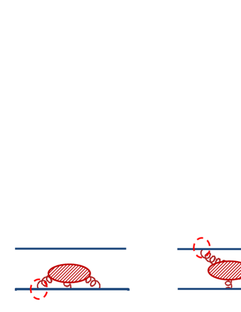
Figure 8: To take into account the couplings of a gluon to the total static currents, both self-energy and potential-energy diagram contributions need to be included, and a cancellation takes place between them in the IR limit of the gluon momentum $|\vec{q}|\to 0$.

This means that a cancellation takes place between these two types of diagrams, since the IR gluon couples to individual diagrams but decouples from the sum of them.

On the other hand, in analogy with classical electrodynamics, gauge field couples to the total charge of the system in the lowest order [$O(r^{0})$] of the multipole expansion:

$$\int d^{3}\vec{x}\,A^{a}_{\mu}(\vec{x},t)\,J^{\mu}_{a}(\vec{x},t)=A^{a}_{0}(\vec{0},t)\int d^{3}\vec{x}\,J^{0}_{a}(\vec{x},t)+O(r^{1})\,,~{}~{}~{}~{}~{}J^{\mu}_{a}=\sum_{i=Q,\bar{Q}}j^{\mu}_{a,i}\,,$$ (72)

which follows from eq. (70). Accordingly, in the pNRQCD Lagrangian (in the static limit), there is no coupling of the singlet field $S$ and the gauge field at the lowest order of the multipole expansion [35]. Hence, the IR cancellation between the self-energy and potential-energy diagrams is explicit at $O(r^{0})$ in the multipole expansion (OPE) of the total energy of a static $Q\bar{Q}$ pair.

Intuitively, IR gluons with wavelengths of order $\Lambda_{\rm QCD}^{-1}(\gg r)$ cannot resolve the color charge of each particle, hence they only see the total charge of the system. More accurately, coupling of IR gluons to the system can be expressed by an expansion in $\vec{r}$ (multipole expansion) for small $r$, in which the zeroth multipole (=total charge) of the color-singlet $Q\bar{Q}$ pair is zero.

The modern approach (after around 1998) to use the $\overline{\rm MS}$ mass for the computation of $E_{\rm tot}(r)=2m_{\rm pole}+V_{S}(r)$ for a heavy quarkonium system can be viewed as follows. The total energy of the system is computed as the sum of (i) the $\overline{\rm MS}$ masses of $Q$ and $\bar{Q}$, (ii) contributions to the self-energies of $Q$ and $\bar{Q}$ which are not included in the $\overline{\rm MS}$ masses, and (iii) the potential energy between $Q$ and $\bar{Q}$. Contributions of IR gluons with wavelengths larger than $r$ automatically cancel between (ii) and (iii) in this computation [51]. In this way we can eliminate a large part of the IR contributions from the computation of $E_{\rm tot}(r)$.

Appendix B: Derivation of eq. (50)

We show some details of the derivation of eq. (50). The regularized dimensionless potential is given by

$$v_{+} = \int_{0}^{\exp(+i\epsilon)\times\infty}dt\,e^{-t/\alpha_{s}}\,B_{v}(t)$$ (73)

$$= -\frac{2C_{F}}{\pi}\int_{0}^{\exp(+i\epsilon)\times\infty}dt\,e^{-t/\alpha_{s}}\,\int_{0}^{\infty}\frac{dq}{q}\,\sin(qr)B_{\widetilde{\alpha}_{V}(q)}(t)$$

$$= -\frac{2C_{F}}{\pi}i\int_{0}^{\infty}ds\,e^{-is/\alpha_{s}}\,\int_{0}^{\infty}\frac{dq}{q}\,\sin(qr)B_{\widetilde{\alpha}_{V}(q)}(is)\,.$$

The integral contour of $t$ is rotated to the positive imaginary axis ($t=is$). $v_{-}$ can be obtained by setting $\epsilon\to-\epsilon$ and $s\to-s$ (or, by taking the complex conjugate).

The Borel transform of $\widetilde{\alpha}_{V}(q)$ can be expressed in the integral form as

$$B_{\widetilde{\alpha}_{V}(q)}(is)=\int_{-\infty-i\epsilon}^{+\infty-i\epsilon}\frac{dp}{2\pi i}\,e^{ips}\,\widetilde{\alpha}_{V}(q)\biggr{|}_{\alpha_{s}\to 1/p}\,.$$ (74)

We approximate $\widetilde{\alpha}_{V}(q)$ by $[\widetilde{\alpha}_{V}(q)]_{\text{N${}^{k}$LL}}$. According to our current knowledge of the RG equation at N^kLL, $\alpha_{s}(q)$ diverges at $q=q_{*}$ if the running starts from $\mu>q_{*}$ with the initial condition $\alpha_{s}(\mu)=1/p>0$. In this case there is a singularity on the real axis of $p$, due to the singularity of $\alpha_{s}(q)$. At LL ($k=0$), the singularity is located at $p=b_{0}\log(\mu^{2}/q^{2})$. At N^kLL, the singularity of $p$ is on the real axis for given values of $q(>q_{*})$, $\mu$ and $k$, where the relation is given by $q=q_{*}(\mu,\alpha_{s}(\mu)=1/p;k)$. We are concerned with the case that $q$ is in the vicinity of $q_{*}$, where $\alpha_{s}(q)\sim(q-q_{*})^{-1/(k+1)}$. The singularity of $p$ can be shifted infinitesimally into the upper-half plane (hence, without crossing the contour of $p$ integral) by a shift $q\to q-i\epsilon$ in the vicinity of $q_{*}$.

After changing the order of the integration, we can integrate over $p$ and $s$, which transforms $\widetilde{\alpha}_{V}(q)$ to $\widetilde{\alpha}_{V}(q)$. Then we are left with the $q$ integration with the integral contour deformed into the lower-half plane in the vicinity of $q_{*}$. The above $i\epsilon$-prescription for $q$ specifies how to avoid the singularity of $[\widetilde{\alpha}_{V}(q)]_{\text{N${}^{k}$LL}}$ at $q=q_{*}$ compatibly with the deformation of the integral contour of $t$.

References

- [1] W. Fischler, “Quark - anti-Quark Potential in QCD,” Nucl. Phys. B 129 (1977) 157.
- [2] T. Appelquist, M. Dine and I. J. Muzinich, “The Static Potential In Quantum Chromodynamics,” Phys. Lett. B 69, 231 (1977); T. Appelquist, M. Dine and I. J. Muzinich, “The Static Limit Of Quantum Chromodynamics,” Phys. Rev. D 17, 2074 (1978).
- [3] M. Peter, “The static quark-antiquark potential in QCD to three loops,” Phys. Rev. Lett. 78, 602 (1997) [arXiv:hep-ph/9610209]; M. Peter, “The static potential in QCD: A full two-loop calculation,” Nucl. Phys. B 501, 471 (1997) [arXiv:hep-ph/9702245];
- [4] Y. Schroder, “The static potential in QCD to two loops,” Phys. Lett. B 447, 321 (1999).
- [5] M. Melles, “The static QCD potential in coordinate space with quark masses through two loops,” Phys. Rev. D 62, 074019 (2000); [arXiv:hep-ph/0001295]. M. Melles, “Two loop mass effects in the static position space QCD-potential,” Nucl. Phys. Proc. Suppl. 96, 472 (2001); [arXiv:hep-ph/0009085].
- [6] A. H. Hoang, “Bottom quark mass from Upsilon mesons: Charm mass effects,” arXiv:hep-ph/0008102.
- [7] S. Recksiegel and Y. Sumino, “Perturbative QCD potential, renormalon cancellation and phenomenological potentials,” Phys. Rev. D 65, 054018 (2002). [arXiv:hep-ph/0109122].
- [8] N. Brambilla, A. Pineda, J. Soto and A. Vairo, “The infrared behaviour of the static potential in perturbative QCD,” Phys. Rev. D 60, 091502 (1999); [arXiv:hep-ph/9903355].
- [9] N. Brambilla, A. Pineda, J. Soto and A. Vairo, “Potential NRQCD: An Effective theory for heavy quarkonium,” Nucl. Phys. B 566, 275 (2000) doi:10.1016/S0550-3213(99)00693-8 [hep-ph/9907240].
- [10] B. A. Kniehl and A. A. Penin, “Ultrasoft effects in heavy quarkonium physics,” Nucl. Phys. B 563, 200 (1999). [arXiv:hep-ph/9907489].
- [11] N. Brambilla, X. Garcia i Tormo, J. Soto and A. Vairo, “The Logarithmic contribution to the QCD static energy at N4LO,” Phys. Lett. B 647, 185 (2007) [hep-ph/0610143].
- [12] A. Pineda and J. Soto, “The Renormalization group improvement of the QCD static potentials,” Phys. Lett. B 495, 323 (2000) doi:10.1016/S0370-2693(00)01261-2 [hep-ph/0007197].
- [13] N. Brambilla, A. Vairo, X. Garcia i Tormo and J. Soto, “The QCD static energy at NNNLL,” Phys. Rev. D 80, 034016 (2009) doi:10.1103/PhysRevD.80.034016 [arXiv:0906.1390 [hep-ph]].
- [14] A. V. Smirnov, V. A. Smirnov and M. Steinhauser, “Fermionic contributions to the three-loop static potential,” Phys. Lett. B 668, 293 (2008). [arXiv:0809.1927 [hep-ph]].
- [15] C. Anzai, Y. Kiyo and Y. Sumino, “Static QCD potential at three-loop order,” Phys. Rev. Lett. 104, 112003 (2010) [arXiv:0911.4335 [hep-ph]];
- [16] A. V. Smirnov, V. A. Smirnov and M. Steinhauser, “Three-loop static potential,” Phys. Rev. Lett. 104, 112002 (2010) [arXiv:0911.4742 [hep-ph]].
- [17] R. N. Lee, A. V. Smirnov, V. A. Smirnov and M. Steinhauser, “Analytic three-loop static potential,” Phys. Rev. D 94, no. 5, 054029 (2016) [arXiv:1608.02603 [hep-ph]].
- [18] C. Ayala, G. Cvetič and A. Pineda, “The bottom quark mass from the system at NNNLO,” JHEP 1409, 045 (2014) [arXiv:1407.2128 [hep-ph]].
- [19] A. Hoang, P. Ruiz-Femenia and M. Stahlhofen, “Renormalization Group Improved Bottom Mass from Upsilon Sum Rules at NNLL Order,” JHEP 1210, 188 (2012); [arXiv:1209.0450 [hep-ph]],
- [20] C. Ayala and G. Cvetič, “Calculation of binding energies and masses of quarkonia in analytic QCD models,” Phys. Rev. D 87, 054008 (2013); [arXiv:1210.6117 [hep-ph]].
- [21] A. A. Penin and N. Zerf, “Bottom Quark Mass from Sum Rules to ,” JHEP 1404, 120 (2014);
- [22] M. Beneke, A. Maier, J. Piclum and T. Rauh, “The bottom-quark mass from non-relativistic sum rules at NNNLO,” Nucl. Phys. B 891 (2015) 42. [arXiv:1411.3132 [hep-ph]].
- [23] Y. Kiyo, G. Mishima and Y. Sumino, “Determination of and from quarkonium energy levels in perturbative QCD,” Phys. Lett. B 752, 122 (2016) Erratum: [Phys. Lett. B 772, 878 (2017)] [arXiv:1510.07072 [hep-ph]].
- [24] C. Peset, A. Pineda and J. Segovia, “The charm/bottom quark mass from heavy quarkonium at N3LO,” JHEP 1809, 167 (2018) [arXiv:1806.05197 [hep-ph]].
- [25] V. Mateu and P. G. Ortega, “Bottom and Charm Mass determinations from global fits to bound states at N3LO,” JHEP 1801, 122 (2018) [arXiv:1711.05755 [hep-ph]].
- [26] Y. Kiyo, G. Mishima and Y. Sumino, “Strong IR Cancellation in Heavy Quarkonium and Precise Top Mass Determination,” JHEP 1511, 084 (2015) [arXiv:1506.06542 [hep-ph]].
- [27] S. Kawabata and H. Yokoya, “Top-quark mass from the diphoton mass spectrum,” Eur. Phys. J. C 77, no. 5, 323 (2017) [arXiv:1607.00990 [hep-ph]].
- [28] A. Bazavov, N. Brambilla, X. Garcia i Tormo, P. Petreczky, J. Soto and A. Vairo, “Determination of from the QCD static energy: An update,” Phys. Rev. D 90, no. 7, 074038 (2014) [arXiv:1407.8437 [hep-ph]]. A. Bazavov, N. Brambilla, X. G. Tormo, I, P. Petreczky, J. Soto, A. Vairo and J. H. Weber, “Determination of the QCD coupling from the static energy and the free energy,” arXiv:1907.11747 [hep-lat].
- [29] H. Takaura, T. Kaneko, Y. Kiyo and Y. Sumino, “Determination of from static QCD potential with renormalon subtraction,” Phys. Lett. B 789, 598 (2019) [arXiv:1808.01632 [hep-ph]]. H. Takaura, T. Kaneko, Y. Kiyo and Y. Sumino, “Determination of from static QCD potential: OPE with renormalon subtraction and lattice QCD,” JHEP 1904, 155 (2019) [arXiv:1808.01643 [hep-ph]].
- [30] M. Beneke, “Renormalons,” Phys. Rept. 317, 1 (1999).
- [31] A. Pineda, “Heavy Quarkonium And Nonrelativistic Effective Field Theories,” Ph.D. Thesis (1998).
- [32] A. H. Hoang, M. C. Smith, T. Stelzer and S. Willenbrock, “Quarkonia and the pole mass,” Phys. Rev. D 59, 114014 (1999); [arXiv:hep-ph/9804227].
- [33] M. Beneke, “A quark mass definition adequate for threshold problems,” Phys. Lett. B 434, 115 (1998). [arXiv:hep-ph/9804241].
- [34] C. Bauer, G. S. Bali and A. Pineda, “Compelling Evidence of Renormalons in QCD from High Order Perturbative Expansions,” Phys. Rev. Lett. 108, 242002 (2012) [arXiv:1111.3946 [hep-ph]].
- [35] N. Brambilla, A. Pineda, J. Soto and A. Vairo, “Effective field theories for heavy quarkonium,” Rev. Mod. Phys. 77 (2005) 1423. [arXiv:hep-ph/0410047].
- [36] T. Lee, “Renormalons beyond one loop,” Phys. Rev. D 56, 1091 (1997) [hep-th/9611010].
- [37] A. Pineda, “Determination of the bottom quark mass from the Upsilon(1S) system,” JHEP 0106, 022 (2001) [hep-ph/0105008].
- [38] Y. Sumino, Lecture Note, “Understanding Interquark Force and Quark Masses in Perturbative QCD,” arXiv:1411.7853 [hep-ph].
- [39] M. Beneke and V. A. Smirnov, Nucl. Phys. B 522, 321 (1998) doi:10.1016/S0550-3213(98)00138-2 [hep-ph/9711391].
- [40] A. S. Kronfeld, “The Perturbative pole mass in QCD,” Phys. Rev. D 58, 051501 (1998) doi:10.1103/PhysRevD.58.051501 [hep-ph/9805215].
- [41] Y. Sumino, “’Coulomb + linear’ form of the static QCD potential in operator product expansion,” Phys. Lett. B 595, 387 (2004) [hep-ph/0403242].
- [42] A. Pineda, Phys. Rev. D 84, 014012 (2011) doi:10.1103/PhysRevD.84.014012 [arXiv:1101.3269 [hep-ph]].
- [43] H. Takaura, “Renormalon free part of an ultrasoft correction to the static QCD potential,” Phys. Lett. B 783, 350 (2018) [arXiv:1712.05435 [hep-ph]].
- [44] M. B. Voloshin, “On Dynamics of Heavy Quarks in Nonperturbative QCD Vacuum,” Nucl. Phys. B 154, 365 (1979). doi:10.1016/0550-3213(79)90037-3
- [45] H. Leutwyler, “How to Use Heavy Quarks to Probe the QCD Vacuum,” Phys. Lett. 98B, 447 (1981). doi:10.1016/0370-2693(81)90450-0
- [46] C. A. Flory, “The Static Potential in Quantum Chromodynamics,” Phys. Lett. 113B, 263 (1982). doi:10.1016/0370-2693(82)90835-8
- [47] Y. Sumino, “QCD potential as a ’Coulomb plus linear’ potential,” Phys. Lett. B 571, 173 (2003) [hep-ph/0303120].
- [48] Y. Sumino, “Static QCD Potential at : perturbative expansion and operator-product expansion,” Phys. Rev. D 76, 114009 (2007). [arXiv:hep-ph/0505034].
- [49] K. Melnikov and T. v. Ritbergen, “The Three loop relation between the MS-bar and the pole quark masses,” Phys. Lett. B 482, 99 (2000) doi:10.1016/S0370-2693(00)00507-4 [hep-ph/9912391].
- [50] P. Marquard, A. V. Smirnov, V. A. Smirnov, M. Steinhauser and D. Wellmann, “-on-shell quark mass relation up to four loops in QCD and a general SU gauge group,” Phys. Rev. D 94, no. 7, 074025 (2016) doi:10.1103/PhysRevD.94.074025 [arXiv:1606.06754 [hep-ph]].
- [51] N. Brambilla, Y. Sumino and A. Vairo, “Quarkonium spectroscopy and perturbative QCD: A New perspective,” Phys. Lett. B 513, 381 (2001) doi:10.1016/S0370-2693(01)00611-6 [hep-ph/0101305].