Average search time bounds in cue based search strategy

Vaibhav Wasnik wasnik@iitgoa.ac.in Indian Institute of Technology, Goa
Abstract

In this work we consider the problem of searches that utilizes past information gathered during searching, to evaluate the probability distribution of finding the source at each step. We start with a sample strategy where the movement at each step is in the immediate neighborhood direction, with a probability proportional to the normalized difference in probability of finding the source with the present position source finding probability. We evaluate a lower bound for the average search time for this strategy. We next consider the problem of the lower bound on any strategy that utilities information of the probability distribution evaluated by the searcher at any instant. We derive an expression for the same. Finally we present an analytic expression for this lower bound in the case of homogeneous diffusion of particles by a source. For a general probability distribution with entropy -$E$, we find that the lowerbound goes as $e^{E/2}$.

Introduction:- Searching for a source that emits particles is a problem that is quite ubiquitous. We see this all the way from a bacteria searching for the source of chemoattractants chemotaxis , to a robot figuring out the source of a gas leak in a room robot . Search time is defined as the time required to find the source by a searcher. This is similar to the first passage time: the first time the searcher reaches the position occupied by the source. There is a lot of theoretical work done in this area redner . One could classify search strategies into two broad categories. Searches with cues and searches without cues. Searches without cues are reviewed in benichou . As has been stated there, searches with cues can also be split up into two kinds. One of them involves chemotatic strategies that assume a sufficient concentration of cues and another category of strategies that involve searching through information coming from sparse cues. Infotaxis infotaxis falls in the later category.

A searcher moving through an environment of particles emitted by a source has a history of hits at times $t_{1},..,t_{n}$ at positions $\vec{r}(t_{1}),...,\vec{r}(t_{n})$. These make up the cues that provide all the information from the environment. This information could be utilized in deciding a future direction in many ways. One important quantity that could be measured is the probability of finding the source at any location in space. One could use Bayes theorem to evaluate this as

$\displaystyle P(\vec{r}|\vec{r}(t_{1}),...,\vec{r}(t_{n}))=\frac{P(\vec{r}(t_{1}),...,\vec{r}(t_{n}))|\vec{r})}{\sum_{x}P(\vec{r}(t_{1}),...,\vec{r}(t_{n}))|\vec{x})}$ (1)

here $P(\vec{r}|\vec{r}(t_{1}),...,\vec{r}(t_{n})$ is the probability of finding the source at position $\vec{r}$ given hits at positions $\vec{r}(t_{1}),...,\vec{r}(t_{n})$ and $P(\vec{r}(t_{1}),...,\vec{r}(t_{n}))|\vec{x})$ is probability of hits happening at positions $\vec{r}(t_{1}),...,\vec{r}(t_{n}))$ given the source is at position $\vec{x}$. Infotaxis infotaxis utilizes this probability to evaluate the entropy of the source. The motion of the searcher at each step is in a direction in which the expected information gain is a maximum. In infotaxis it was conveyed that evaluating the search time analytically for a searcher undergoing Infotaxis, was difficult, given the complexity of the search algorithm. Given this issue, the question arises whether it would be possible to evaluate the search times for a class of cue based searches and any statement be made about certain universal features, such as lower bound on these search times given certain constraints. In this work we begin with a strategy that utilizes past cues to evaluate the probability distribution of finding the source at each step and where the searcher at each step moves in the immediate neighborhood, with a probability proportional to the normalized difference in probability of finding the source with the present position source finding probability. We then attempt to evaluate a lower bound on the search times in case of homogeous diffusion of particles by a source. We then consider the problem of the lower bound on any strategy that utilities information of the probability distribution evaluated by the searcher at any instant. We evaluate an analytical expression for lower bound in case of homogeneous diffusion of particles by a source. For a general probability distribution with entropy -$E$, we find that the lowerbound goes as $e^{E/2}$.

Narrowing the source:-

Let us assume that the source emitting particles is located at the origin. A searcher moving through an environment of particles emitted by a source has a history of hits at times $t_{1},..,t_{n}$ at positions $\vec{r}(t_{1}),...,\vec{r}(t_{n})$. We have,

$\displaystyle P(\vec{r}|\vec{r}(t_{1}),...,\vec{r}(t_{n}))=$
$\displaystyle\frac{\exp[-\int_{0}^{t}P(\vec{r}(t^{\prime})|\vec{r})]dt^{\prime}P(\vec{r}(t_{1}),...,\vec{r}(t_{n}))|\vec{r})}{\sum_{x}\exp[-\int_{0}^{t}P(\vec{r}(t^{\prime})|\vec{x})]dt^{\prime}P(\vec{r}(t_{1}),...,\vec{r}(t_{n}))|\vec{x})}$

Here, $P(\vec{r}(t_{1}),...,\vec{r}(t_{n}))|\vec{r})$ is the probability of having hits at positions $\vec{r}(t_{1}),...,\vec{r}(t_{n}))$ given the source is at position $r$. The exponentials correspond to no hits happening at the other locations along the trajectory. Because the hits are independent of each other and can happen at any time. We could write the above as

$\displaystyle P(\vec{r}|\vec{r_{1}},...,\vec{r_{n}})$
$\displaystyle=\frac{\exp[-\int_{0}^{t}S(\vec{r}(t^{\prime})|\vec{r})dt^{\prime}]S(\vec{r_{1}}|\vec{r})...S(\vec{r_{n}}|\vec{r})}{\sum_{x}\exp[-\int_{0}^{t}S(\vec{r}(t^{\prime})|\vec{x})dt^{\prime}]S(\vec{r_{1}}|\vec{x})..S(\vec{r_{n}}|\vec{x})}$

Where above we $\vec{r_{1}}$..$\vec{r_{n}}$ are just the positions in space, implying that the probability evaluations are only dependent on the positions in space where hits happen irrespective of the time they happen. The $S(\vec{r_{1}}|\vec{x})$ is used above, to imply that the probability of having hits is simply the probability of having particles at location $\vec{r_{1}}$ assuming source is at $\vec{x}$. This assumes that the searcher has an analytical expression for how the particle distribution would be, given the source location.

The probability that the hits happened at these positions is simply

$\displaystyle e^{-\int_{0}^{t}[S(\vec{r}(t^{\prime})|0)]dt^{\prime}}S(\vec{r_{1}}|\vec{0})...S(\vec{r_{n}}|\vec{0})$ (4)

Hence, the average probability of finding the source at $\vec{r}$ would be

P​(rβ†’)=βˆ‘t​r​a​j​e​c​t​o​r​i​e​sβˆ‘n1n!π‘ƒβ†’π‘Ÿsubscriptπ‘‘π‘Ÿπ‘Žπ‘—π‘’π‘π‘‘π‘œπ‘Ÿπ‘–π‘’π‘ subscript𝑛1𝑛\displaystyle P(\vec{r})=\sum_{trajectories}\sum_{n}\frac{1}{n!}
$\displaystyle\sum_{r_{1},..r_{n}}e^{-\int_{0}^{t}[S(\vec{r}(t^{\prime})|\vec{r})+S(\vec{r}(t^{\prime})|0)]dt^{\prime}}S(\vec{r_{1}}|\vec{0})...S(\vec{r_{n}}|\vec{0})$ $\displaystyle\times$
$\displaystyle\frac{S(\vec{r_{1}}|\vec{r})...S(\vec{r_{n}}|\vec{r})}{\sum_{x}e^{-\int_{0}^{t}S(\vec{r}(t^{\prime})|\vec{x})dt^{\prime}}S(\vec{r_{1}}|\vec{x})...S(\vec{r_{n}}|\vec{x})}$

It is obvious that if our trajectory took an infinite time we would have the best narrowing of the source location. Hence, the best possible average probability distribution possible telling us the probability of locating the source at position $\vec{r}$ is

Pβˆžβ€‹(rβ†’)=βˆ‘t​r​a​j​e​c​t​o​r​i​e​sβˆ‘n1n!subscriptπ‘ƒβ†’π‘Ÿsubscriptπ‘‘π‘Ÿπ‘Žπ‘—π‘’π‘π‘‘π‘œπ‘Ÿπ‘–π‘’π‘ subscript𝑛1𝑛\displaystyle P_{\infty}(\vec{r})=\sum_{trajectories}\sum_{n}\frac{1}{n!}
$\displaystyle\sum_{r_{1},..r_{n}}e^{-\int_{0}^{\infty}[S(\vec{r}(t^{\prime})|\vec{r})+S(\vec{r}(t^{\prime})|0)]dt^{\prime}}S(\vec{r_{1}}|\vec{0})...S(\vec{r_{n}}|\vec{0})$ $\displaystyle\times$
$\displaystyle\frac{S(\vec{r_{1}}|\vec{r})...S(\vec{r_{n}}|\vec{r})}{\sum_{x}e^{-\int_{0}^{\infty}S(\vec{r}(t^{\prime})|\vec{x})dt^{\prime}}S(\vec{r_{1}}|\vec{x})...S(\vec{r_{n}}|\vec{x})}$

Let us assume for illustrative purposes that $S(\vec{r_{1}}|\vec{x})=S(|\vec{r_{1}}-\vec{x}|)$. Also, let us assume that $S$ is appreciable only up to a distance $L$ away from the source. One immediately see’s from the above expression that because of presence of terms like $S(\vec{r_{1}}|\vec{0})S(\vec{r_{1}}|\vec{r})$, implies that the average probability distribution of finding the source evaluated above is appreciable over a distance $2L$, as long as we are considering trajectories of lengths or order larger than $L$ . This implies that the probability distribution measured by the searcher will not narrow the source better compared to $S$. If we consider the limit in which $t\rightarrow 0$ in Eq.LABEL:bayes_1, we can see that the probability distribution measured by the searcher is centered at the searcher position. The measured probability distribution is similarly in general not centered at the position of the source for other values of $t$. This implies that the measured probability distribution by the searcher cannot narrow the source better than $S(x)$.

Example Strategy:- Let us consider a search strategy in which the probability to jump to a neighboring location is proportional to the difference in the probability of finding the source from its own location. The probability for the searcher to jump to the nearest neighbor $(x+2dx,y)$ on an average would go as $\beta\;\theta(P(x+2dx,y)-P(x,y))\frac{(P(x+2dx,y)-P(x,y))}{P(x,y)}$. $P(x,y)$ is the average probability of finding the source at position $(x,y)$ that has been evaluated by the searcher using the Baye’s theorem as talked in Eq.LABEL:bayes_1. This could depend on the starting position of the searcher. $\beta$ is a rate at which this jumps happen and $\Theta(x)$ is defined as,

$$\Theta(x)=\begin{cases}1,&\text{if $x>0$}.\\ 0,&\text{otherwise}.\end{cases}$$ (7)

Let us consider the average time to reach the source from position $(x,y)$ as $T(x,y)$. As derived in appendix

$\displaystyle 0$ $\displaystyle=$ $\displaystyle-P(x,y)-2\beta\nabla T(x,y)\cdot\nabla P(x,y)-\beta T(x,y)\nabla^{2}P(x,y)$
$\displaystyle+$ $\displaystyle\alpha\beta\nabla^{2}T(x,y)$

For simplicity let probability distribution have radial symmetry with the source located at $r=0$. Then the above equation simply becomes

$\displaystyle 0$ $\displaystyle=$ $\displaystyle-P(r)-\beta\frac{\partial T(\bar{r})}{\partial r}\frac{\partial P(\bar{r})}{\partial r}-\beta T(\bar{r})[\frac{\partial^{2}P(\bar{r})}{\partial r^{2}}+\frac{1}{r}\frac{\partial P(\bar{r})}{\partial r}]$
$\displaystyle+$ $\displaystyle\alpha\beta P(r)[\frac{\partial^{2}T(\bar{r})}{\partial r^{2}}+\frac{1}{r}\frac{\partial T(\bar{r})}{\partial r}]$

For $\alpha=0$ the solution with $T(r=0)=0$ is

$\displaystyle T(r)$ $\displaystyle=$ $\displaystyle-\frac{1}{\beta rP^{\prime}(r)}\int_{0}^{r}xP(x)dx$ (10)

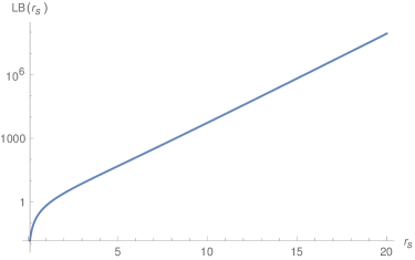
As talked above, the probability distribution $P(x)$ would never be as localized near the source as $S(x)$. In case we are considering homogeneous diffusion by a source at the origin, in two dimensions, the equilibrium particle concentration at $r$ goes as $K_{0}(r/l)$. Hence the lower bound on search time simply is

$\displaystyle T(r)>LB(r)$ $\displaystyle=$ $\displaystyle-\frac{1}{\beta rK_{0}^{\prime}(r/l)}\int_{0}^{r}xK(x/l)dx$ (11)

This is plotted in fig.1. One can see that for large times the $LB(r)$ increases exponentially with $r$. This would be the lower bound even if Ξ±β‰ 0𝛼0\alpha\neq 0, because $\alpha$ only adds randomness to the search and hence would increase the search times.

Refer to caption
Figure 1: $LB(r)$ plotted against $r$ for $l=1$. We see that the lower bound goes exponentially as $r$ at larger values of $r$.

Generic lower bound:- We can simply use the fact that the probability distribution evaluated by Baye’s theorem is not as concentrated near the source as $S(x,y)$ to simply evaluate a lower bound on search time as follows. First let us assume that the searcher knows that the source is located at the origin with a probability $1$. Then the smallest time taken by the searcher to reach the source goes as $r$, the distance between the source and the searcher. In case the searcher instead knowns that the source is located at two points $\vec{x_{1}}$ and $\vec{x_{2}}$ with probability $p_{1}$ and $p_{2}$. Then, the smallest possible search time would simply go as $p_{1}|\vec{x_{1}}-\vec{x_{s}}|+p_{2}|\vec{x_{2}}-\vec{x_{s}}|$ where $\vec{x_{s}}$ is the searchers position. This is obvious because out of $N$ possible measurements, the source is seen at $Np_{1}$ times at $\vec{x_{1}}$ and $Np_{2}$ times at $\vec{x_{2}}$. One could extend this to say that for a source probability distribution $P(\vec{x})$ as understood by the searcher, the shortest time to reach the source on an average should go as $\int d\vec{x}|\vec{x_{s}}-\vec{x}|P(\vec{x})$ .

Since the fact that the probability distribution evaluated by Baye’s theorem is not as concentrated near the source as $S(\vec{x})$, the search time evaluated using any strategy that utilizes the probability distribution as measured by a searcher could never be smaller than $\frac{1}{v_{s}}\int d\vec{x}|\vec{x_{s}}-\vec{x}|S(\vec{x})$ ($v_{s}$ is the speed of the searcher, which we take to be equal to $1$ below), which for $S\sim K_{0}(r/l)$ is

L​B​(rs)𝐿𝐡subscriptπ‘Ÿπ‘ \displaystyle LB(r_{s}) $\displaystyle\sim$ ∫r​𝑑θ​𝑑r​K0​(r/l)​(rsβˆ’r​cos⁑θ)2+r2​sin2β‘ΞΈπ‘Ÿdifferential-dπœƒdifferential-dπ‘Ÿsubscript𝐾0π‘Ÿπ‘™superscriptsubscriptπ‘Ÿπ‘ π‘Ÿπœƒ2superscriptπ‘Ÿ2superscript2πœƒ\displaystyle\int rd\theta drK_{0}(r/l)\sqrt{(r_{s}-r\cos\theta)^{2}+r^{2}\sin^{2}\theta}
$\displaystyle=$ ∫r​𝑑θ​𝑑r​K0​(r/l)​rs2+r2βˆ’2​r​rs​cosβ‘ΞΈπ‘Ÿdifferential-dπœƒdifferential-dπ‘Ÿsubscript𝐾0π‘Ÿπ‘™superscriptsubscriptπ‘Ÿπ‘ 2superscriptπ‘Ÿ22π‘Ÿsubscriptπ‘Ÿπ‘ πœƒ\displaystyle\int rd\theta drK_{0}(r/l)\sqrt{r_{s}^{2}+r^{2}-2rr_{s}\cos\theta}

Now since

1rs2+r2βˆ’2​r​rs​cos⁑θ1superscriptsubscriptπ‘Ÿπ‘ 2superscriptπ‘Ÿ22π‘Ÿsubscriptπ‘Ÿπ‘ πœƒ\displaystyle\frac{1}{\sqrt{r_{s}^{2}+r^{2}-2rr_{s}\cos\theta}} $\displaystyle=$ βˆ‘l=0,∞rlrsl+1​Pl​(cos⁑θ),rs>rsubscript𝑙0superscriptπ‘Ÿπ‘™superscriptsubscriptπ‘Ÿπ‘ π‘™1subscriptπ‘ƒπ‘™πœƒsubscriptπ‘Ÿπ‘ π‘Ÿ\displaystyle\sum_{l=0,\infty}\frac{r^{l}}{r_{s}^{l+1}}P_{l}(\cos\theta),\;r_{s}>r
$\displaystyle=$ βˆ‘l=0,∞rslrl+1​Pl​(cos⁑θ),rs<rsubscript𝑙0superscriptsubscriptπ‘Ÿπ‘ π‘™superscriptπ‘Ÿπ‘™1subscriptπ‘ƒπ‘™πœƒsubscriptπ‘Ÿπ‘ π‘Ÿ\displaystyle\sum_{l=0,\infty}\frac{r_{s}^{l}}{r^{l+1}}P_{l}(\cos\theta),\;r_{s}<r

implies

12​rsβˆ’2​r​cos⁑θ​dd​rs​rs2+r2βˆ’2​r​rs​cos⁑θ12subscriptπ‘Ÿπ‘ 2π‘Ÿπœƒπ‘‘π‘‘subscriptπ‘Ÿπ‘ superscriptsubscriptπ‘Ÿπ‘ 2superscriptπ‘Ÿ22π‘Ÿsubscriptπ‘Ÿπ‘ πœƒ\displaystyle\frac{1}{2r_{s}-2r\cos\theta}\frac{d}{dr_{s}}\sqrt{r_{s}^{2}+r^{2}-2rr_{s}\cos\theta} $\displaystyle=$ βˆ‘l=0,∞rlrsl+1​Pl​(cos⁑θ),rs>rsubscript𝑙0superscriptπ‘Ÿπ‘™superscriptsubscriptπ‘Ÿπ‘ π‘™1subscriptπ‘ƒπ‘™πœƒsubscriptπ‘Ÿπ‘ π‘Ÿ\displaystyle\sum_{l=0,\infty}\frac{r^{l}}{r_{s}^{l+1}}P_{l}(\cos\theta),\;r_{s}>r
$\displaystyle=$ βˆ‘l=0,∞rslrl+1​Pl​(cos⁑θ),rs<rsubscript𝑙0superscriptsubscriptπ‘Ÿπ‘ π‘™superscriptπ‘Ÿπ‘™1subscriptπ‘ƒπ‘™πœƒsubscriptπ‘Ÿπ‘ π‘Ÿ\displaystyle\sum_{l=0,\infty}\frac{r_{s}^{l}}{r^{l+1}}P_{l}(\cos\theta),\;r_{s}<r

Hence

d​L​B​(rs)d​rs𝑑𝐿𝐡subscriptπ‘Ÿπ‘ π‘‘subscriptπ‘Ÿπ‘ \displaystyle\frac{dLB(r_{s})}{dr_{s}} $\displaystyle=$ ∫0rs∫02​πr​𝑑θ​𝑑r​K0​(r/l)β€‹βˆ‘l=0,∞2​(rsβˆ’r​cos⁑θ)​rlrsl+1superscriptsubscript0subscriptπ‘Ÿπ‘ superscriptsubscript02πœ‹π‘Ÿdifferential-dπœƒdifferential-dπ‘Ÿsubscript𝐾0π‘Ÿπ‘™subscript𝑙02subscriptπ‘Ÿπ‘ π‘Ÿπœƒsuperscriptπ‘Ÿπ‘™superscriptsubscriptπ‘Ÿπ‘ π‘™1\displaystyle\int_{0}^{r_{s}}\int_{0}^{2\pi}rd\theta drK_{0}(r/l)\sum_{l=0,\infty}\frac{2(r_{s}-r\cos\theta)r^{l}}{r_{s}^{l+1}}
Pl​(cos⁑θ)+∫rs∞∫02​πr​𝑑θ​𝑑rsubscriptπ‘ƒπ‘™πœƒsuperscriptsubscriptsubscriptπ‘Ÿπ‘ superscriptsubscript02πœ‹π‘Ÿdifferential-dπœƒdifferential-dπ‘Ÿ\displaystyle P_{l}(\cos\theta)+\int_{r_{s}}^{\infty}\int_{0}^{2\pi}rd\theta dr
K0​(r/l)β€‹βˆ‘l=0,∞2​(rsβˆ’r​cos⁑θ)​rslrl+1​Pl​(cos⁑θ)subscript𝐾0π‘Ÿπ‘™subscript𝑙02subscriptπ‘Ÿπ‘ π‘Ÿπœƒsuperscriptsubscriptπ‘Ÿπ‘ π‘™superscriptπ‘Ÿπ‘™1subscriptπ‘ƒπ‘™πœƒ\displaystyle K_{0}(r/l)\sum_{l=0,\infty}\frac{2(r_{s}-r\cos\theta)r_{s}^{l}}{r^{l+1}}P_{l}(\cos\theta)
(15)

For large values of rssubscriptπ‘Ÿπ‘ r_{s}, the second integral would contribute minisculely. Also majority contribution in first term would only show from the $l=0$. Hence

d​L​B​(rs)d​rs𝑑𝐿𝐡subscriptπ‘Ÿπ‘ π‘‘subscriptπ‘Ÿπ‘ \displaystyle\frac{dLB(r_{s})}{dr_{s}} $\displaystyle\approx$ 2Γ—2β€‹Ο€β€‹βˆ«0rsr​𝑑r​K0​(r/l)Γ—rsrs22πœ‹superscriptsubscript0subscriptπ‘Ÿπ‘ π‘Ÿdifferential-dπ‘Ÿsubscript𝐾0π‘Ÿπ‘™subscriptπ‘Ÿπ‘ subscriptπ‘Ÿπ‘ \displaystyle 2\times 2\pi\int_{0}^{r_{s}}rdrK_{0}(r/l)\times\frac{r_{s}}{r_{s}}
$\displaystyle\approx$ $\displaystyle 4\pi l^{2}$

As rssubscriptπ‘Ÿπ‘ r_{s} is made smaller, other contributions start appearing. However, we note that as rssubscriptπ‘Ÿπ‘ r_{s} becomes larger and larger, the lower bound on search time goes simply as rssubscriptπ‘Ÿπ‘ r_{s}. This simply states the fact that as rssubscriptπ‘Ÿπ‘ r_{s} becomes large, the range over which the region of size $l$ surrounding the source looks like a point object to the searcher. This behavior is seen by solving Eq.2 for $l=1$ as plotted in fig. 2.

For small values of rssubscriptπ‘Ÿπ‘ r_{s} one could simply expand

L​B​(rs)𝐿𝐡subscriptπ‘Ÿπ‘ \displaystyle LB(r_{s}) $\displaystyle\sim$ ∫r​𝑑θ​𝑑r​K0​(r/l)​rs2+r2βˆ’2​r​rs​cosβ‘ΞΈπ‘Ÿdifferential-dπœƒdifferential-dπ‘Ÿsubscript𝐾0π‘Ÿπ‘™superscriptsubscriptπ‘Ÿπ‘ 2superscriptπ‘Ÿ22π‘Ÿsubscriptπ‘Ÿπ‘ πœƒ\displaystyle\int rd\theta drK_{0}(r/l)\sqrt{r_{s}^{2}+r^{2}-2rr_{s}\cos\theta} (17)
$\displaystyle=$ ∫r2​𝑑θ​𝑑r​K0​(r/l)​1+rs2r2βˆ’2​rsr​cos⁑θsuperscriptπ‘Ÿ2differential-dπœƒdifferential-dπ‘Ÿsubscript𝐾0π‘Ÿπ‘™1superscriptsubscriptπ‘Ÿπ‘ 2superscriptπ‘Ÿ22subscriptπ‘Ÿπ‘ π‘Ÿπœƒ\displaystyle\int r^{2}d\theta drK_{0}(r/l)\sqrt{1+\frac{r_{s}^{2}}{r^{2}}-2\frac{r_{s}}{r}\cos\theta}
$\displaystyle=$ ∫0∞∫02​π𝑑θ​𝑑r​K0​(r/l)​(rs22+r2βˆ’22​rs28​cos2⁑θ)superscriptsubscript0superscriptsubscript02πœ‹differential-dπœƒdifferential-dπ‘Ÿsubscript𝐾0π‘Ÿπ‘™superscriptsubscriptπ‘Ÿπ‘ 22superscriptπ‘Ÿ2superscript22superscriptsubscriptπ‘Ÿπ‘ 28superscript2πœƒ\displaystyle\int_{0}^{\infty}\int_{0}^{2\pi}d\theta drK_{0}(r/l)(\frac{r_{s}^{2}}{2}+r^{2}-2^{2}\frac{r_{s}^{2}}{8}\cos^{2}\theta)
$\displaystyle=$ ∫0∞∫02​π𝑑θ​𝑑r​K0​(r/l)​(rs2​sin2⁑θ2+r2)superscriptsubscript0superscriptsubscript02πœ‹differential-dπœƒdifferential-dπ‘Ÿsubscript𝐾0π‘Ÿπ‘™superscriptsubscriptπ‘Ÿπ‘ 2superscript2πœƒ2superscriptπ‘Ÿ2\displaystyle\int_{0}^{\infty}\int_{0}^{2\pi}d\theta drK_{0}(r/l)(\frac{r_{s}^{2}\sin^{2}\theta}{2}+r^{2})
$\displaystyle=$ 2​π​π2​l3+12​π​π​l2​rs22πœ‹πœ‹2superscript𝑙312πœ‹πœ‹π‘™2superscriptsubscriptπ‘Ÿπ‘ 2\displaystyle 2\pi\frac{\pi}{2}l^{3}+\frac{1}{2}\pi\frac{\pi l}{2}r_{s}^{2}
$\displaystyle=$ Ο€2​l3+.25​π2​l​rs2superscriptπœ‹2superscript𝑙3.25superscriptπœ‹2𝑙superscriptsubscriptπ‘Ÿπ‘ 2\displaystyle\pi^{2}l^{3}+.25\pi^{2}lr_{s}^{2}

which is the behavior for rs<<lmuch-less-thansubscriptπ‘Ÿπ‘ π‘™r_{s}<<l. Note that

L​B​(rs)𝐿𝐡subscriptπ‘Ÿπ‘ \displaystyle LB(r_{s}) $\displaystyle\sim$ ∫r​𝑑θ​𝑑r​K0​(r/l)​(rsβˆ’r​cos⁑θ)2+r2​sin2β‘ΞΈπ‘Ÿdifferential-dπœƒdifferential-dπ‘Ÿsubscript𝐾0π‘Ÿπ‘™superscriptsubscriptπ‘Ÿπ‘ π‘Ÿπœƒ2superscriptπ‘Ÿ2superscript2πœƒ\displaystyle\int rd\theta drK_{0}(r/l)\sqrt{(r_{s}-r\cos\theta)^{2}+r^{2}\sin^{2}\theta}
$\displaystyle=$ l3β€‹βˆ«rl​𝑑θ​𝑑rl​K0​(r/l)​(rsl)2+(rl)2βˆ’2​rl​rsl​cos⁑θsuperscript𝑙3π‘Ÿπ‘™differential-dπœƒdifferential-dπ‘Ÿπ‘™subscript𝐾0π‘Ÿπ‘™superscriptsubscriptπ‘Ÿπ‘ π‘™2superscriptπ‘Ÿπ‘™22π‘Ÿπ‘™subscriptπ‘Ÿπ‘ π‘™πœƒ\displaystyle l^{3}\int\frac{r}{l}d\theta d\frac{r}{l}K_{0}(r/l)\sqrt{(\frac{r_{s}}{l})^{2}+(\frac{r}{l})^{2}-2\frac{r}{l}\frac{r_{s}}{l}\cos\theta}
$\displaystyle=$ l3β€‹βˆ«x​𝑑θ​𝑑x​K0​(x)​(rsl)2+x2βˆ’2​x​rsl​cos⁑θsuperscript𝑙3π‘₯differential-dπœƒdifferential-dπ‘₯subscript𝐾0π‘₯superscriptsubscriptπ‘Ÿπ‘ π‘™2superscriptπ‘₯22π‘₯subscriptπ‘Ÿπ‘ π‘™πœƒ\displaystyle l^{3}\int xd\theta dxK_{0}(x)\sqrt{(\frac{r_{s}}{l})^{2}+x^{2}-2x\frac{r_{s}}{l}\cos\theta}

Hence all that matters is how rssubscriptπ‘Ÿπ‘ r_{s} compares to $l$. From fig.2 we can see that when rs>2​lsubscriptπ‘Ÿπ‘ 2𝑙r_{s}>2l, the behavior of L​B​(rs)𝐿𝐡subscriptπ‘Ÿπ‘ LB(r_{s}) is linear. From Eq.LABEL:slope we can see that slope of this line is $4\pi l^{2}$. One can hence say that

L​B​(rs)>Ο€2​l32+4​π​l2​rs𝐿𝐡subscriptπ‘Ÿπ‘ superscriptπœ‹2superscript𝑙324πœ‹superscript𝑙2subscriptπ‘Ÿπ‘ \displaystyle LB(r_{s})>\frac{\pi^{2}l^{3}}{2}+4\pi l^{2}r_{s} (19)
Refer to caption
Figure 2: L​B​(rs)𝐿𝐡subscriptπ‘Ÿπ‘ LB(r_{s}) plotted as a function of rssubscriptπ‘Ÿπ‘ r_{s} solving Eq.2 with $l=1$. As can be seen at large values of rs>lsubscriptπ‘Ÿπ‘ π‘™r_{s}>l we have an expected lower bound going as rssubscriptπ‘Ÿπ‘ r_{s}. Also note that for rs=0subscriptπ‘Ÿπ‘ 0r_{s}=0 the lower bound on the search time is not zero.

If we instead consider the lower bound on search time given a particular entropy of the source probability distribution we have to minimize

$\displaystyle LB$ $\displaystyle=$ $\displaystyle\int 2\pi rdrd\theta rS(r,\theta)-\lambda\int 2\pi rdrd\theta(S(r,\theta)\ln S(r,\theta)+E)$
$\displaystyle-\beta(\int 2\pi rdrd\theta S(r,\theta)-1)$

We have assumed the searcher is located at $r=0$. Here $\lambda$ is the Lagrange multiplier that sets $E$ to the entropy of the probability distribution $S(r,\theta)$. Minimizing w.r.t $S(r,\theta)$ gives

$\displaystyle r-\lambda(\ln S(r,\theta)+1)-\beta$ $\displaystyle=$ $\displaystyle 0$

which solves to

$\displaystyle S(r,\theta)=e^{r/\lambda-\beta/\lambda-1}$ (22)

$\lambda<0$ for consistency. Requiring that

$\displaystyle\int 2\pi rdrd\theta(S(r,\theta)\ln S(r,\theta))$ $\displaystyle=$ $\displaystyle-E$
$\displaystyle\rightarrow(2\pi)^{2}\lambda e^{\frac{\beta}{\lambda}-1}(\beta-3\lambda)=-E$
$\displaystyle\int 2\pi rdrd\theta S(r,\theta)$ $\displaystyle=$ $\displaystyle 1\rightarrow e^{\beta/\lambda-1}(2\pi)^{2}\lambda^{2}=1$

which implies $(\beta-3\lambda)=-E\lambda\rightarrow(\frac{\beta}{\lambda})=3-E$ and $\lambda=-\frac{1}{2\pi}e^{E/2-1}$

Hence the lower bound is

$\displaystyle LB$ $\displaystyle=$ $\displaystyle\int 2\pi rdrd\theta rS(r,\theta)=-2(2\pi)^{2}\lambda^{3}e^{\frac{\beta}{\lambda}-1}=-2\lambda=\frac{e^{E/2-1}}{\pi}$

Conclusion:- In infotaxis the difficulty in evaluating the search time for Infotaxis was highlighted. and instead a calculation for a different search strategy, which does not utilize information about past hits, was presented. They evaluated the lower limit for search time for this strategy in certain limits as $\sim e^{E}$, where $-E$ is the entropy of the probability distribution of finding the source. We however have in this work we evaluated a lower bound on the average search time in a search strategy that seeks to evaluate the probability distribution of finding the source, given the information of past hits, such that rate of jumps to a neibhouring site is proportional to the normalized difference of evaluated probability of finding the source with the present site of the searcher. This lowerbound goes as the exponential of distance from the source for large distances. We then provided an expression for the lower bound for the search time for any cues based search strategy. For a general probability distribution with entropy -$E$, we showed that the lowerbound goes as $e^{E/2}$. We see that the lowerbound again goes as $e^{E/2}$ which is similar to $e^{E}$ in ref.infotaxis , which was evaluated for a non cue based search strategy for the limit in which the search time as well as entropy are much larger than $1$. The similarity almost begs a conjecture that for probability distributions that do not narrow the source position well, cue based searches do not perform appreciably better than non cue based searches. It would be interesting to further explore this statement through further research.

Appendix:- To simplify things, let us consider the system in one dimension. The final result can be easily generalized to higher dimensions. We have

$\displaystyle T(x)$ $\displaystyle=$ $\displaystyle-dt+T(x+dx)[\beta\Pi(x+dx)+\alpha\Delta(x+dx)]$
$\displaystyle+$ $\displaystyle T(x-dx)[\beta\Pi(x-dx)+\alpha\Delta(x-dx)]$
$\displaystyle+$ T​(x)​[1βˆ’Ξ²β€‹(Π​(x+d​x)βˆ’+Π​(xβˆ’d​x)βˆ’+2​α​Δ​(x))]𝑇π‘₯delimited-[]1𝛽Πsuperscriptπ‘₯𝑑π‘₯Ξ superscriptπ‘₯𝑑π‘₯2𝛼Δπ‘₯\displaystyle T(x)[1-\beta(\Pi(x+dx)^{-}+\Pi(x-dx)^{-}+2\alpha\Delta(x))]

where

$\displaystyle\Pi(i)$ $\displaystyle=$ $\displaystyle\Theta(P(x)-P(i))\frac{(P(x)-P(i))}{P(x)}$
Π​(i)βˆ’Ξ superscript𝑖\displaystyle\Pi(i)^{-} $\displaystyle=$ $\displaystyle\Theta(-P(x)+P(i))\frac{(-P(x)+P(i))}{P(x)}$
$\displaystyle\Delta(i)$ $\displaystyle=$ $\displaystyle 1\quad P(x)=P(i)$
$\displaystyle=$ 0P​(x)β‰ P​(i)0𝑃π‘₯𝑃𝑖\displaystyle 0\quad P(x)\neq P(i)

The eq. LABEL:eq simply states that we can reach point $x$ from any of its neighbors $x+dx$ and $x-dx$, which subtracts time $dt$ from times $T(x+dx)$ , $T(x-dx)$ to reach source from these sites. Each of the times $T(x+dx)$ , $T(x-dx)$ are multiplied by the probabilities to make the jump from $x+dx$ and $x-dx$ to $x$ respectively. The term multiplying $T(x)$ on the RHS is simply the probability of not making a jump to the neighbors $x+dx$,$x-dx$. $\alpha$ is the probability of making a jump randomly in case the neibhouring site has the same probability of finding the source as present site.

This eq. LABEL:eq becomes

$\displaystyle 0$ $\displaystyle=$ βˆ’d​t+β​[T​(x+d​x)​Π​(x+d​x)+T​(xβˆ’d​x)​Π​(xβˆ’d​x)]𝑑𝑑𝛽delimited-[]𝑇π‘₯𝑑π‘₯Ξ π‘₯𝑑π‘₯𝑇π‘₯𝑑π‘₯Ξ π‘₯𝑑π‘₯\displaystyle-dt+\beta\;[T(x+dx)\Pi(x+dx)+T(x-dx)\Pi(x-dx)]
$\displaystyle-$ T​(x)​β​[(Π​(x+d​x)βˆ’+Π​(xβˆ’d​x)βˆ’)]+β​α​d​x2β€‹βˆ‡2T​(x)𝑇π‘₯𝛽delimited-[]Ξ superscriptπ‘₯𝑑π‘₯Ξ superscriptπ‘₯𝑑π‘₯𝛽𝛼𝑑superscriptπ‘₯2superscriptβˆ‡2𝑇π‘₯\displaystyle T(x)\beta[(\Pi(x+dx)^{-}+\Pi(x-dx)^{-})]+\beta\alpha dx^{2}\nabla^{2}T(x)

or

$\displaystyle 0$ $\displaystyle=$ βˆ’dt+Ξ²[(T(x)+dxβˆ‚xT(x))Ξ (x+dx)\displaystyle-dt+\beta\;[(T(x)+dx\partial_{x}T(x))\Pi(x+dx)
$\displaystyle+$ (T(x)βˆ’dxβˆ‚xT(x))Ξ (xβˆ’dx)]\displaystyle(T(x)-dx\partial_{x}T(x))\Pi(x-dx)]
$\displaystyle-$ T​(x)​β​[(Π​(x+d​x)βˆ’+Π​(xβˆ’d​x)βˆ’)]+β​α​d​x2β€‹βˆ‡2T​(x)𝑇π‘₯𝛽delimited-[]Ξ superscriptπ‘₯𝑑π‘₯Ξ superscriptπ‘₯𝑑π‘₯𝛽𝛼𝑑superscriptπ‘₯2superscriptβˆ‡2𝑇π‘₯\displaystyle T(x)\beta[(\Pi(x+dx)^{-}+\Pi(x-dx)^{-})]+\beta\alpha dx^{2}\nabla^{2}T(x)

or

$\displaystyle 0$ $\displaystyle=$ $\displaystyle-dt-\beta\;dx^{2}\;\partial_{x}T(x)[\frac{\partial_{x}P(x)}{P(x)}\Theta(P(x)-P(x+dx))$
$\displaystyle+$ $\displaystyle\frac{\partial_{x}P(x)}{P(x)}\Theta(P(x)-P(x-dx))]$
$\displaystyle+$ T​(x)​β​[(Π​(x+d​x)+Π​(xβˆ’d​x))]𝑇π‘₯𝛽delimited-[]Ξ π‘₯𝑑π‘₯Ξ π‘₯𝑑π‘₯\displaystyle T(x)\beta[(\Pi(x+dx)+\Pi(x-dx))]
$\displaystyle-$ T​(x)​β​[(Π​(x+d​x)βˆ’+Π​(xβˆ’d​x)βˆ’)]+β​α​d​x2β€‹βˆ‡2T​(x)𝑇π‘₯𝛽delimited-[]Ξ superscriptπ‘₯𝑑π‘₯Ξ superscriptπ‘₯𝑑π‘₯𝛽𝛼𝑑superscriptπ‘₯2superscriptβˆ‡2𝑇π‘₯\displaystyle T(x)\beta[(\Pi(x+dx)^{-}+\Pi(x-dx)^{-})]+\beta\alpha dx^{2}\nabla^{2}T(x)

now

Π​(i)βˆ’Ξ β€‹(i)βˆ’Ξ π‘–Ξ superscript𝑖\displaystyle\Pi(i)-\Pi(i)^{-} $\displaystyle=$ $\displaystyle[\Theta(P(x)-P(i))+\Theta(-P(x)+P(i)))]$
$\displaystyle\frac{(P(x)-P(i))}{P(x)}=\frac{(P(x)-P(i))}{P(x)}$

hence

$\displaystyle 0$ $\displaystyle=$ $\displaystyle-dt-\beta\;dx^{2}\;\partial_{x}T(x)\frac{\partial_{x}P(x)}{P(x)}$
$\displaystyle-$ $\displaystyle T(x)\beta[\frac{(P(x+dx)+P(x-dx)-2P(x)}{P(x)}]+\beta\alpha dx^{2}\nabla^{2}T(x)$

or

$\displaystyle 0$ $\displaystyle=$ $\displaystyle-P(x)dt-\beta\;dx^{2}\;\partial_{x}T(x)\partial_{x}P(x)$
$\displaystyle-$ $\displaystyle T(x)\beta\;dx^{2}\;\nabla^{2}P(x)+\beta\alpha dx^{2}P(x)\nabla^{2}T(x)$

which becomes in higher dimensions

$\displaystyle 0$ $\displaystyle=$ $\displaystyle-P(x)-\beta\nabla T(x)\cdot\nabla P(x)$
$\displaystyle-$ $\displaystyle\beta T(x)\nabla^{2}P(x)+\beta\alpha P(x)\nabla^{2}T(x)$

we have redefined $\frac{\beta dx^{2}}{dt}\rightarrow\beta$ above.

References

  • (1) Eisenbach, M., Lengeler, J. W., Varon, M., Gutnick, D., Meili, R., Firtel, R. A., … , Murakami, F. (2004). Chemotaxis.
  • (2) Ishida, H., Ushiku, T., Toyama, S., Taniguchi, H., Moriizumi, T. (2005). Mobile robot path planning using vision and olfaction to search for a gas source. In SENSORS, 2005 IEEE (pp. 4-pp). IEEE.
  • (3) Redner, Sidney. A guide to first-passage processes. Cambridge University Press, 2001.
  • (4) BΓ©nichou, Olivier, et al. ”Intermittent search strategies.” Reviews of Modern Physics 83.1 (2011): 81.
  • (5) Vergassola, Massimo, Emmanuel Villermaux, and Boris I. Shraiman. β€β€˜Infotaxis’ as a strategy for searching without gradients.” Nature 445.7126 (2007): 406.