SAINT: Spatially Aware Interpolation NeTwork for Medical Slice Synthesis

Abstract

Deep learning-based single image super-resolution (SISR) methods face various challenges when applied to 3D medical volumetric data (i.e., CT and MR images) due to the high memory cost and anisotropic resolution, which adversely affect their performance. Furthermore, mainstream SISR methods are designed to work over specific upsampling factors, which makes them ineffective in clinical practice. In this paper, we introduce a Spatially Aware Interpolation NeTwork (SAINT) for medical slice synthesis to alleviate the memory constraint that volumetric data poses. Compared to other super-resolution methods, SAINT utilizes voxel spacing information to provide desirable levels of details, and allows for the upsampling factor to be determined on the fly. Our evaluations based on 853 CT scans from four datasets that contain liver, colon, hepatic vessels, and kidneys show that SAINT consistently outperforms other SISR methods in terms of medical slice synthesis quality, while using only a single model to deal with different upsampling factors.

1 Introduction

Medical imaging methods such as computational tomography (CT) and magnetic resonance imaging (MRI) are essential to modern day diagnosis and surgery planning. To provide necessary visual information of the human body, it is desirable to acquire high resolution and high contrast medical images. For MRI, the acquisition of higher resolution images take a long time, and thus, practitioners often accelerate the process by acquiring fewer slices.

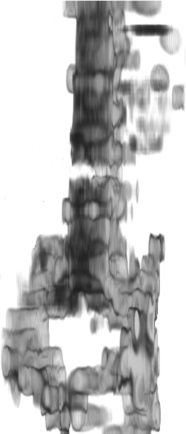
(a) Bicubical Interpolation

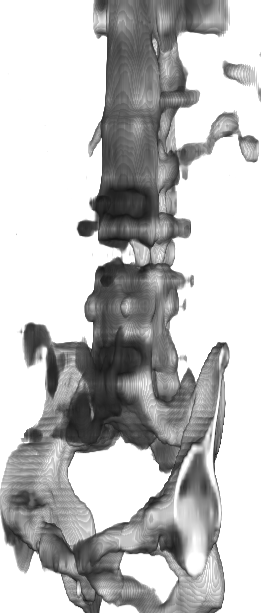
(b) mDCSRN[4]

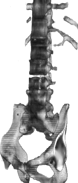
(c) 3D RDN [27]

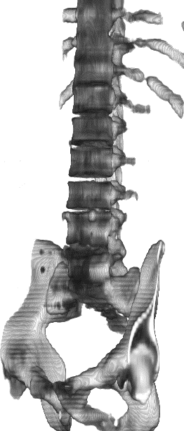
(d) SAINT (Ours)

Figure 1: 3D renderings of bones from CT slice interpolation results. Bicubical interpolation (a) from sparsely sampled CT volume, with highly unrealistic distortions. Methods (b) and (c) improve the image quality; however, they are still under-resolved as is evident on the spinal column. SAINT (d) resolves details much better on the spinal column.

CT image acquisition is much faster than MRI; however, due to the high cost of keeping complete 3D volumes in memory and print, typically only necessary number of slices are stored. As a result, most medical imaging volumes are anisotropic, with high within-slice resolution and low between-slice resolution. The inconsistent resolution leads to a range of issues, from unpleasant viewing experience to difficulties in developing robust analysis algorithms. Currently, many datasets [9, 19, 1] use affine transforms to equalize voxel spacing between volumes, which may introduce significant distortions to the original data, as shown in Fig. 1(a). Therefore, methods for some analysis tasks, e.g. lesion segmentation, have to resort to intricate algorithms to take into account of the change in resolution[18, 22, 16]. As such, an accurate and reliable 3D SISR method to upsample the low between-slice resolution, which we refer to as the slice interpolation task, is much needed.

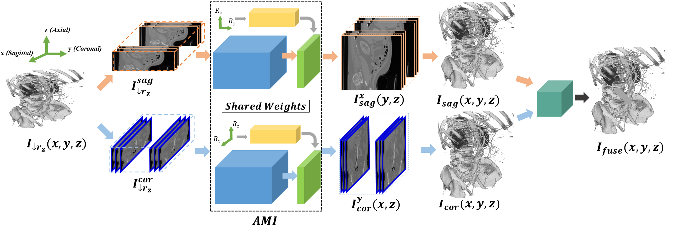
Figure 2: The overall pipeline of Spatially Aware Interpolation NeTwork (SAINT). For visualization purpose, the volumes are rendered in 3D based on their bone structures.

Implementations of 3D SISR model suffer from various problems. Firstly, medical images are volumetric and three dimensional in nature, which often lead to memory bottlenecks with Deep Learning (DL)-based methods. While it is possible to mitigate the issue by patch-based training, such an approach will produce undesirable artifact when the patches are stitched together at inference time. Therefore, compared to their 2D counterparts, the depth or width of 3D SISR models as well as their input sample size must be reconciled. Secondly, a practical slice interpolation model also needs to robustly handle different levels of upsampling factors without retraining to adapt to various clinical requirements. Most SISR methods can only recover images from one downsampling level (e.g. $\times$2 or $\times$4), which is insufficient for real application. A recent method by Hu et al. [10] allows for arbitrary magnification factor through a meta-learning upsampling structure. Unfortunately, in order to achieve this functionality, the method requires to generate a filter for every pixel which is extremely memory intensive. Finally, mainstream SISR methods do not consider the underlying physical resolution of the images. Since medical images are often anisotropic in physical resolution to different degrees, a new formulation to address the physical resolution may potentially increase the sensitivity of the output.

To address these problems, we propose a Spatially Aware Interpolation NeTwork (SAINT), an efficient approach to upsample 3D CT images by treating between-slices images through 2D CNN networks. This resolves the memory bottleneck and associated stitching artifacts. To address the anisotropic resolution issue, SAINT introduces an Anisotropic Meta Interpolation (AMI) mechanism, which is inspired by Meta-SR [10] that uses a filter-generating meta network to enable flexible upsampling rates. Instead of using the input-output pixel mapping as in Meta-SR, AMI uses a new image-wide projection that accounts for the spatial resolution variations in medical images and allows arbitrary upsampling factors in integers.

SAINT then introduces a Residual-Fusion Network (RFN) that eliminates the inconsistencies resulting from applying AMI (which addresses images in 2D) to 3D CT images, and incorporates information from the third axis for improved modeling of 3D context. Benefited by the effective interpolation of AMI, RFN is lightweight and converges quickly. Combining AMI and RFN, SAINT not only significantly resolves the memory bottleneck at inference time, allowing for deeper and wider networks for 3D SISR, but also provides improved performance, as shown in Fig. 1.

In summary, our main contributions are listed below:

• We propose a unified 3D slice interpolation framework called SAINT for anisotropic volumes. This approach is scalable in terms of memory and removes the stitching artifacts created by 3D methods.

• We propose a 2D SISR network called Anisotropic Meta Interpolation (AMI), which upsample the between-slice images from anisotropic volumes. It handles different upsampling factors with a single model, incorporates the spatial resolution knowledge, and generates far less filter weights compared to Meta-SR.

• We propose a Residual-Fusion Network (RFN), which fuses the volumes produced by AMI by refining on details of the synthesized slices through residual learning.

• We examine the proposed SAINT network through extensive evaluation on 853 CT scans from four datasets that contain liver, colon, hepatic vessels, and kidneys and demonstrate its superior performance quantitatively. SAINT performs consistently well on independent datasets and on unseen upsampling factor, which further validates its applicability in practice.

2 Related Work

Two dimensional DL-based SISR has achieved great improvements compared to conventional interpolation methods. Here we focus on the most recent advances on natural image SISR, and their applications in medical imaging, such as in reconstruction and denoising.

2.1 Natural Image SISR

Dong et al.[5] first proposed SRCNN, which learns a mapping that transforms LR images to HR images through a three layer CNN. Many subsequent studies explored strategies to improve SISR such as using deeper architectures and weight-sharing[13, 26, 14]. However, these methods require interpolation as a pre-processing step, which drastically increases computational complexity and leads to noise in data. To address this issue, Dong et al.[6] proposed to apply deconvolution layers for LR image to be directly upsampled to finer resolution. Shi et al.[20] first proposed ESPCN, which allows for real-time super-resolution by using a sub-pixel convolutional layer and a periodic shuffling operator to upsample image at the end of the network. Furthermore, many studies have shown that residual learning provided better performance in SISR[17, 15, 27]. Specifically, Zhang et al.[27] incorporated both residual learning and dense blocks[11], and introduced Residual Dense Blocks (RDB) to allow for all layers of features to be seen directly by other layers, achieving state-of-the-art performance.

Besides performance, flexibility in upsampling factor has been studied to enable faster deployment and improved robustness. Lim et al.[17] proposed a variant of their EDSR method called MDSR to create individual substructures within the model to accommodate for different upsampling factors. Jo et al.[12] employed dynamic upsampling filters for video super-resolution and generated the filters based on the neighboring frame of each pixel in LR frames in order to achieve better detail resolution. Hu et al.[10] proposed Meta-SR to dynamically generate filters for every LR-SR pixel pair, thus allowing for arbitrary upsampling factors.

Generative Adversarial Networks (GAN)[7] have also been incorporated in SISR to improve the visual quality of the generated images. Ledig et al. pointed out that training SISR networks solely by $L_{1}$ loss intrinsically leads to blurry estimations, and proposed SRGAN[15] to generate more detail-rich images despite the lower PSNR values.

2.2 CT Image Quality Improvement

There is a long history of research on accelerating CT acquisition due to its practical importance. More recently, much of the attention has been put on faster acceleration with noisy data followed by high quality recovery with CNN based methods. For CT acquisition, the applications range from denoising low-intensity, low dose CT images[29, 3, 24], to improving quality of reconstructed images from sparse-view and limited-angle data[28, 2, 25, 8]. A variety of network structures has been experimented, including the encoder-decoder (UNet), DenseNet, and GAN structure. Similar to the SRGAN, networks that involve GAN[24] report inferior PSNR values, and superior visual details. We refrain from applying GAN loss in our model, as it may produce unexplainable artifacts. We mainly focus on pixel-wise L1 loss in our work.

While most work focuses on improving 2D medical image quality, Chen et al.[4] proposed mDCSRN, which uses a 3D variant of DenseNet for super-resolving MR images. In order to resolve the memory bottleneck, mDCSRN applies inference through patches of smaller 3D cubes, and pads each patch with three pixels of neighboring cubes to avoid distortion. Similar approaches were used by Wang et al.[23]. Wolterink et al.[24] resolved such issues through supplying CNN network with few slices, and applying 3D kernels only in the lower layers.

3 Spatially Aware Interpolation Network

Let $I(x,y,z)\in\mathbb{R}^{X\times Y\times Z}$ denote a densely sampled CT volume. By convention, we refer to the $x$ axis as the “sagittal” axis, the $y$ axis as the “coronal” axis, and the $z$ axis as the “axial” axis. Accordingly, there are three types of slices:

• The sagittal slice for a given $x$: $I^{x}(y,z)=I(x,y,z),~{}\forall x$.

• The coronal slice for a given $y$: $I^{y}(x,z)=I(x,y,z),~{}\forall y$.

• The axial slice for a given $z$: $I^{z}(x,y)=I(x,y,z),~{}\forall z$.

Without loss of generality, this work considers slice interpolation along the axial axis. For a densely-sampled CT volume $I(x,y,z)$, the corresponding sparsely-sampled volume is defined as

$$I_{\downarrow r_{z}}(x,y,z)=I(x,y,r_{z}\cdot z),$$ (1)

where $I_{\downarrow r_{z}}(x,y,z)\in\mathbb{R}^{X\times Y\times\frac{Z}{r_{z}}}$, and $r_{z}$ is the sparsity factor along the $z$ axis from $I(x,y,z)$ to $I_{\downarrow r_{z}}(x,y,z)$ and the upsampling factor from $I_{\downarrow r_{z}}(x,y,z)$ to $I(x,y,z)$.

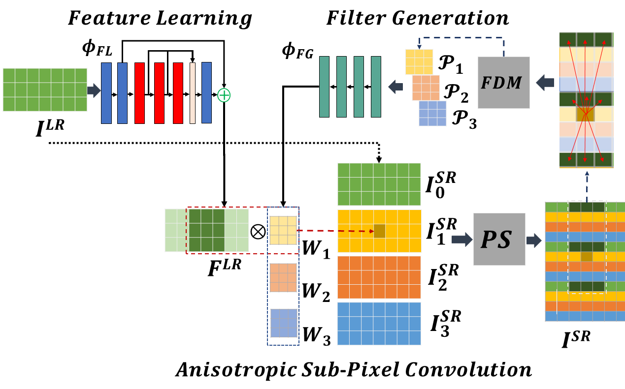
Figure 3: AMI architecture. The feature learning stage generates $F^{LR}$ from $I^{LR}$. Based on the dynamically determined $r_{z}$, the filter generation stage generates filters $W_{c}$, which are convolved with $F^{LR}$ to produce $I^{SR}_{c}$. $I^{SR}_{c}$ is then rearranged for the final $I^{SR}$. The physical distance between the $I^{LR}$ coordinates and the generated $I^{SR}_{c}$ pixel coordinate is mapped through FDM and provided to the filter generation stage. This figure demonstrates the process when the upsampling factor $r_{z}=4$ and filter size $k=3$

The goal of slice interpolation is to find a transformation $\mathcal{T}\colon{\mathbb{R}^{X\times Y\times\frac{Z}{r_{z}}}}\to{\mathbb{R}^{X\times Y\times Z}}$ that can optimally transform $I_{\downarrow r_{z}}(x,y,z)$ back to $I(x,y,z)$ for an arbitrary integer $r_{z}$.

3.1 Overview of the Proposed Method

As shown in Fig. 2, SAINT consists of two stages: Anisotropic Meta Interpolation (AMI) and Residual Fusion Network (RFN).

Given $I_{\downarrow r_{z}}(x,y,z)$, we view it as a sequence of 2D sagittal slices $I^{x}_{\downarrow r_{z}}(y,z)$ marginally from the sagittal axis. The same volume can also be treated as $I^{y}_{\downarrow r_{z}}(x,z)$ from the coronal axis. Interpolating $I^{x}_{\downarrow r_{z}}(y,z)$ to $I^{x}(y,z)$ and $I^{y}_{\downarrow r_{z}}(x,z)$ to $I^{y}(x,z)$ are equivalent to applying a sequence of 2D super-resolution along the $x$ axis and $y$ axis, respectively. We apply AMI $\mathcal{G}_{\theta}$ to upsample $I^{x}_{\downarrow r_{z}}(y,z)$ and $I^{y}_{\downarrow r_{z}}(x,z)$ as follows:

$$I^{x}_{sag}(y,z)=\mathcal{G}_{\theta}(I^{x}_{\downarrow r_{z}}(y,z)),~{}I^{y}_{cor}(x,z)=\mathcal{G}_{\theta}(I^{y}_{\downarrow r_{z}}(x,z)).$$ (2)

The super-resolved slices are reformatted as sagittally and coronally super-resolved volumes $I_{sag}(x,y,z)$, $I_{cor}(x,y,z)$, and resampled axially to obtain $I_{sag}^{z}(x,y)$, $I_{cor}^{z}(x,y)$. We apply RFN $\mathcal{F}_{\theta}$ to fuse $I_{sag}^{z}(x,y)$ and $I_{cor}^{z}(x,y)$ together, such that:

$$I^{z}_{fuse}(x,y)=\mathcal{F}_{\theta}(I_{sag}^{z}(x,y),I_{cor}^{z}(x,y)),$$ (3)

and obtain our final synthesized slices $I^{z}_{fuse}(x,y)$.

3.2 Anisotropic Meta Interpolation

We break down $\mathcal{G}_{\theta}$ into three parts: (i) the Feature Learning (FL) stage $\phi_{FL}$, which extracts features from LR images using an architecture adopted from RDN[27], (ii) the Filter Generation (FG) stage $\phi_{FG}$, which enables arbitrary upsampling factor by generating convolutional filters of different sizes, and (iii) Anisotropic Sub-Pixel Convolution, which performs sub-pixel convolution and periodic shuffling (PS) operations to produce the final output.

3.2.1 Feature Learning

Given an input low-resolution image $I^{LR}\in\{I^{x}_{\downarrow r_{z}}(y,z),I^{y}_{\downarrow r_{z}}(x,z)\}$, the feature learning (FL) stage simply extracts its feature maps $F^{LR}$:

$$F^{LR}=\phi_{FL}(I^{LR};\theta_{FL}),$$ (4)

where $\theta_{FL}$ is the parameter of the filter learning network $\phi_{FL}$. Note that $F^{LR}\in\{F^{x}_{\downarrow r_{z}}(y,z),F^{y}_{\downarrow r_{z}}(x,z)\}$. For the same brevity in notation, we also use $I^{SR}\in\{I^{x}_{sag}(y,z),I^{y}_{cor}(x,z)\}$ to denote the corresponding super-resolved image obtained in (2).

3.2.2 Anisotropic Sub-Pixel Convolution

Mainstream SISR methods use sub-pixel convolution [20] to achieve isotropic upsampling. In order to achieve anisotropic upsampling, we define upsampling factor along the $z$ dimension as $r_{z}$. As shown in Fig. 3, our anisotropic sub-pixel convolution layer takes a low-resolution image $I^{LR}\in\mathbb{R}^{H\times W}$ and its corresponding feature $F^{LR}\in\mathbb{R}^{C^{\prime}\times H\times r_{z}W}$ as the inputs and outputs a super-resolved image $I^{SR}\in\mathbb{R}^{H\times r_{z}W}$. Formally, this layer performs the following operations:

$$I_{0}^{SR}=I^{LR},I_{c}^{SR}=F^{LR}\circledast W_{c},$$ (5)

$$I^{SR}=PS([I_{0}^{SR},I_{1}^{SR},\dots,I_{r_{z}-1}^{SR}]),$$ (6)

where $\circledast$ and $[\dots]$ denote the convolution and channel-wise concatenation operation, respectively. $W_{c},c\in\{1,\dots,r_{z}-1\}$ denotes the convolution kernel whose construction will be discussed in Section 3.2.3. The convolution operation aims to output $I^{SR}_{c}$, which is an interpolated slice of $I^{LR}$. Concatenating the input $I^{LR}=I_{0}^{SR}$ with the interpolated slices $\{I^{SR}_{1},\dots,I^{SR}_{r_{z}-1}\}$, we obtain an $r_{z}\times H\times W$ tensor and then apply periodic shuffling (PS) to reshape the tensor for the super-resolved image $I^{SR}$.

3.2.3 Filter Generation

Inspired by Meta-SR[10], which employs a meta module to generate convolutional filters, we design a FG stage with a CNN structure that can dynamically generate $W$. Moreover, we propose a Filter Distance Matrix (FDM) operator, which provides a representation of the physical distance between the observed voxels in $I^{SR}_{0}$ and the interpolated voxels in $\{I^{SR}_{1},\dots,I^{SR}_{r_{z}-1}\}$.

Filter Distance Matrix We denote the spatial resolution of $I^{SR}$ as $(R_{h},R_{w})$. As shown in Fig. 3, for each convolution operation in $F^{LR}\circledast W_{c}$, a $k\times k$ patch from $F^{LR}$ is taken to generate a voxel on $I^{SR}_{c}$. To find the distance relationship among them, we first calculate the coordinate distance between every point from the feature patch, which are generated from $I^{LR}$, and the point of the output voxel in $I^{SR}_{c}$, in terms of their rearranged coordinate positions in the final image $I^{SR}$. The coordinate distance is then multiplied by the spatial resolution $(R_{h},R_{w})$, thus yielding a physical distance representation between the pair.

Specifically, we define the PS rearrangement mapping between coordinates in $I^{SR}_{c}$ and in $I^{SR}$ as $\mathcal{M}_{c}$, such that $I^{SR}_{c}(h,w)=I^{SR}(\mathcal{M}_{c}(h,w))$. Mathematically, $\mathcal{M}$ can be expressed as:

$$\mathcal{M}_{c}(h,w)=(h+c,wr_{z}+\left\lfloor\frac{c}{r_{z}}\right\rfloor).$$ (7)

We record the physical distance in a matrix called FDM, denoted as $\mathcal{P}=[P_{1},\dots,P_{r-1}]$. The algorithm to generate $\mathcal{P}_{c}$ for every channel $c$ is shown in Algorithm 1.

Input: target channel: $c$, filter size: $k$, spatial resolution: ($R_{H}$,$R_{W}$), PS mapping: $\mathcal{M}$

Output: FDM for $c$: $\mathcal{P}_{c}$

for h=0:1:$k$ do

       for w=0:1:$k$ do

             $\mathcal{P}_{c}(h,w)$ = $\lVert(\mathcal{M}_{0}(h,w)-\mathcal{M}_{c}(\left\lfloor\frac{k}{2}\right\rfloor,\left\lfloor\frac{k}{2}\right\rfloor))\cdot(R_{H},R_{W})\rVert_{2}$

       end for

      

end for

Algorithm 1 Filter Distance Matrix

$\mathcal{P}_{c}\in\mathbb{R}^{k\times k}$ is a compact representation that has three desirable properties: (i) it embeds the spatial resolution information of a given slice; (ii) it is variant to channel positions; and (iii) it is invariant to coordinate positions. These properties make $\mathcal{P}_{c}$ a suitable input to generate channel-specific filters that can change based on different spatial resolution.

As such, we provide $\mathcal{P}_{c}$ to a filter generation CNN model $\phi_{FG}$ to estimate $W_{c}\in\mathbb{R}^{C^{\prime}\times 1\times k\times k}$, formulated as follows:

$$W_{c}=\phi_{FG}(\mathcal{P}_{c};\theta_{FG})$$ (8)

where $\theta_{FG}$ is the parameter of the filter generation network and $W_{c}$ is the filter weight that produces $I^{SR}_{c}$. We refer the readers to supplemental material section that explains how the changes in $\mathcal{P}$ impact the rate of interpolation for AMI.

Note that instead of super-resolving a 2D slice independently of its neighboring slices, we in practice estimate a single SR slice output by taking three consecutive slices to AMI as inputs to allow more context. After applying the AMI module for all $x$ in $I^{x}_{sag}$ and all $y$ in $I^{y}_{cor}$, we finally reformat the sagittally and coronally super-resolved slices into volumes, $I_{sag}(x,y,z)$ and $I_{cor}(x,y,z)$, respectively. We apply the $L_{1}$ loss in (9) to train AMI:

$$\mathcal{L}_{AMI} =\lVert\mathcal{G}_{\theta}(I^{x}_{\downarrow r_{z}})-I^{x}_{gt}\rVert_{1}+\lVert\mathcal{G}_{\theta}(I^{y}_{\downarrow r_{z}})-I^{y}_{gt}\rVert_{1},$$ (9)

where $I^{x}_{gt}=I^{x}(y,z)$ and $I^{y}_{gt}=I^{y}(x,z)$ in the densely-sampled volume $I$. From the axial perspective, $I_{sag}(x,y,z)$ and $I_{cor}(x,y,z)$ provide line-by-line estimations for the missing axial slices. However, since no constraint is enforced on the estimated axial slices, inconsistent interpolations lead to noticeable artifacts, as shown in Fig. 4. We resolve this problem in the RFN stage of the proposed pipeline.

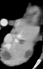
(a) $I_{sag}^{z}(x,y)$

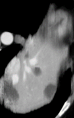
(b) $I_{cor}^{z}(x,y)$

(c) $I_{avg}^{z}(x,y)$

(d) $I_{fuse}(x,y)$

Figure 4: (a) The axial slice generated from $I_{sag}$. (b) The axial slice generated from $I_{cor}$. Some details are better resolved by (a) and others by (b). Both of them exhibit directional artifact due to a lack of constraints in the (x,y) plane. This is resolved through RFN in (d), which refines their average $I_{avg}$, as shown in (c)

3.3 Residual-Fusion Network

Figure 5: RFN architecture

RFN further improves the quality of slice interpolation by learning the structural variations within individual slices. As shown in Fig. 5, we first take the axial slices of the sagitally and coronally super-resovled volumes $I_{sag}(x,y,z)$ and $I_{cor}(x,y,z)$ to obtain $I_{sag}^{z}(x,y)$ and $I_{cor}^{z}(x,y)$, respectively. As each pixel from $I_{sag}^{z}(x,y)$ and $I_{cor}^{z}(x,y)$ represents the best estimate from the sagittal and coronal directions, an average of the slices $I_{avg}^{z}(x,y)$ can reduce some of the directional artifacts. We then apply residual learning, which has been proven to be effective in many image-to-image tasks [17, 15, 27], with fusion network $\mathcal{F_{\phi}}$:

$$I^{z}_{fuse}(x,y)=I^{z}_{avg}(x,y)+\mathcal{F_{\phi}}(I^{z}_{sag}(x,y),I^{z}_{cor}(x,y)),$$ (10)

where $I^{z}_{fuse}(x,y)=\mathcal{F}_{\phi}(I_{sag}^{z},I_{cor}^{z})$ is the output of the fusion network. The objective function for training the fusion network is:

$$\mathcal{L}_{fuse} =\lVert I^{z}_{fuse}(x,y)-I^{z}_{gt}\rVert_{1},$$ (11)

where $I^{z}_{gt}=I^{z}(x,y)$ is from the densely-sampled CT volume. After training, the fusion network is applied to all the synthesized slices $I_{sag}^{z}$ and $I_{cor}^{z}$, yielding CT volume $I_{fuse}(x,y,z)$.

Alternative implementations We experimented with an augmented version of SAINT, where $I(x,y,z)$ is viewed from four different directions by AMI, instead of two, and found minor improvement quantitatively. Furthermore, we also experimented with a 3D version of RFN, where all the filters are changed from 2D to 3D, and found no improvement. We believe that, as AMI is optimized on expanding slices in the axial axis, the produced volumes are already axially consistent. We refer readers to the supplemental material for more details on relevant experiments.

4 Experiments

Implementation Details. We implement the proposed framework using PyTorch. To ensure a fair comparison, we construct all models to have similar number of network parameters and network depth; the network parameters are included in Table 4 and Table 2. For AMI, we use six Residual Dense Blocks (RDBs), eight convolutional layers per RDB, and growth rate of thirty-two for each layer. For the 3D version of RDN, we change to growth rate to sixteen to compensate for the larger 3D kernels. For mDCSRN [4], due to different acquisition methods of CT and MRI, we replace the last convolution layer with RDN’s upsampling module instead of performing spectral downsampling on LR images. We train all the models with Adam optimization, with a momentum of 0.5 and a learning rate of 0.0001, until they converge. For more details on model architectures, please refer to the supplemental material section.

3D volumes take large amount of memory to be directly inferred through deep 3D CNN networks. For mDCSRN, we follow the patch-based algorithm discussed in [4] to break down the volumes into cubes of shape $64\times 64\times 64$, and infer them with margin of three pixels on every side; for other non-SAINT 3D networks, we infer only the central $256\times 256\times Z$ patch to ameliorate the memory issue. Quantitative results of all the methods are calculated on the central $256\times 256\times Z$ patch.

Dataset. We employ 853 CT scans from the publicly available Medical Segmentation Decathlon[21] and 2019 Kidney Tumor Segmentation Challenge (KiTS[9], which we refer to as the kidney dataset hereafter). More specifically, we use the liver, colon, hepatic vessels datasets from Medical Segmentation Decathlon, and take 463 volumes from them for training, 40 for validation, and 351 for testing. The liver dataset contains a mix of volumes with 1mm and 4-5mm slice thickness, colon and hepatic vessels datasets contain volumes with 4-5mm slice thickness. In order to examine the robustness of model performance on unseen data, we also add thirty-two CT volumes from the liver dataset for evaluation, with slice thickness less commonly seen in other datasets.

All volumes have slice dimension of $512\times 512$, with slice resolution ranging from 0.5mm to 1mm, and slice thickness from 0.7mm to 6mm. For data augmentation, all dense CT volumes are downsampled in the slice dimension to enrich volumes of lesser slice resolution. Such data augmentation is performed until either the volume has less than sixty slices, or its slice thickness is more than 5mm.

Evaluation Metrics. We compare different super-resolution approaches using two types of quantitative metrics. Firstly, we use Peak Signal-to-Noise Ratio (PSNR) and Structured Similarity Index (SSIM) to measure low-level image quality. For experiments, we down-sample the original volumes by factors of $r_{z}=4$ and $r_{z}=6$.

4.1 Ablation Study

In this section, we evaluate the effectiveness of AMI against alternative implementations. Specifically, we compare its performance against:

Scale	PSNR/SSIM	Parameters	Liver	Colon	Hepatic Vessels	Kidney
x2	2D MDSR	2.92M	37.17/0.9728	36.74/0.9741	36.80/0.9767	38.81/0.9752
	2D RDN	2.77M	38.50/0.9800	38.11/0.9805	38.36/0.9837	40.09/0.9800
	Meta-SR	2.81M	38.03/0.9770	37.69/0.9785	38.03/0.9818	39.69/0.9776
	AMI	2.81M	38.64/0.9808	38.34/0.9815	38.48/0.9840	40.33/0.9807
	AMI+RFN	2.93M	39.16/0.9826	38.91/0.9835	39.13/0.9858	40.82/0.9821
x4	2D MDSR	2.92M	33.43/0.9471	32.76/0.9436	32.91/0.9490	34.57/0.9508
	2D RDN	2.77M	34.22/0.9546	33.39/0.9511	33.74/0.9571	35.17/0.9550
	Meta-SR	2.81M	34.20/0.9541	33.51/0.9516	33.74/0.9570	35.08/0.9544
	AMI	2.81M	34.40/0.9561	33.65/0.9529	33.93/0.9586	35.28/0.9560
	AMI+RFN	2.93M	34.91/0.9603	34.19/0.9579	34.48/0.9630	35.79/0.9597
x6	2D MDSR	2.92M	31.15/0.9237	30.16/0.9133	30.22/0.9216	32.30/0.9297
	2D RDN	2.77M	31.78/0.9315	30.82/0.9232	31.13/0.9319	32.47/0.9314
	Meta-SR	2.81M	31.88/0.9322	30.86/0.9234	31.09/0.9318	32.60/0.9329
	AMI	2.81M	32.05/0.9333	30.99/0.9249	31.22/0.9333	32.72/0.9343
	AMI+RFN	2.93M	32.50/0.9392	31.50/0.9320	31.89/0.9401	33.22/0.9393

Table 1: Quantitative Comparison of SAINT (AMI+RFN) against alternative methods. The best results are in bold, and the second best results are underlined.

HR

HRPSNR/SSIM

2D MDSR x424.01/0.7735

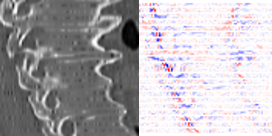
2D RDN x424.42/0.8101

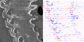
Meta-SR x424.51/0.7995

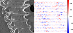
AMI x425.84/0.8414

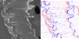
2D MDSR x619.75/0.4727

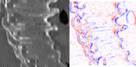
2D RDN x619.22/0.4482

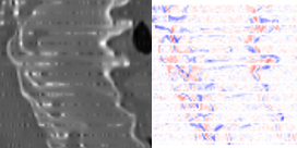
Meta-SR x622.81/0.7069

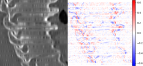
AMI x623.42/0.7376

Figure 6: Visual comparisons of different methods against AMI. The difference maps are provided to the right of the results for better visualization. Images are best viewed when magnified.

1. MDSR: Proposed by Lim et al. [17], MDSR can super-resolve images with multiple upsampling factors.

2. RDN: The original RDN architecture, which allows for fixed upsampling factors.

3. Meta-SR: Using the same RDN structure for feature learning, Meta-SR dynamically generates convolutional kernels based on Location Projection for the last stage.

Table 4 summarizes the performance of different implementations against AMI, evaluated on $I_{sag}(x,y,z)$, which we find to have better quantitative results than $I_{cor}(x,y,z)$ for all methods. For both $r_{z}=4$ and $r_{z}=6$, we found improvement in image quality from AMI over other methods, while Meta-SR and RDN have comparable performance. Despite the higher parameter number, MDSR ranked last due to using different substructures for different upsampling factors. For visual demonstration, we can see in Fig. 6 that AMI is able to recover the separation between the bones of the spine, while other methods lead to erroneous recovery where the bones are merged together. Compared to Meta-SR, AMI generates $HW$ times less filter weights in its filter generation stage. With finite memory, this allows for GPUs to handle more slices in parallel, and achieve faster inference time per volume.

To examine the robustness of different methods, in addition to $r_{z}=4$ and $r_{z}=6$, we also tested the methods on $r_{z}=2$, which is not included in training. AMI and Meta-SR can dynamically adjust the upsampling factor by changing the input to the filter generation network. For 2D MDSR and 2D RDN, we use the $r_{z}=4$ version of the networks to over-upsample $I^{x}_{\downarrow r_{z}=2}(y,z)$ and $I^{y}_{\downarrow r_{z}=2}(x,z)$, and downsample the output by factor of two axially to obtain results. We observe significant degradation in Meta-SR’s performance as compared to other methods. Since Meta-SR’s input to its filter generation stage is dependent on the upsampling factor, an unseen upsampling factor can negatively affect the quality of the generated filters. In comparison, AMI does not explicitly include upsampling factor in its filter generation input, and performs robustly on the unseen upsampling factor.

Scale	PSNR/SSIM	Parameters	Liver	Colon	Hepatic Vessels	Kidney
x4	Bicubic	N/A	28.36/0.8733	28.01/0.8622	27.83/0.8720	30.33/0.8946
	3D MDSR	2.88M	33.70/0.9487	32.79/0.9442	32.80/0.9480	35.36/0.9563
	mDCSRN	2.98M	33.70/0.9494	32.83/0.9455	32.76/0.9487	35.44/0.9572
	3D RDN	2.88M	34.12/0.9535	33.21/0.9497	33.26/0.9538	35.60/0.9582
	SAINT	2.93M	34.91/0.9603	34.19/0.9579	34.48/0.9630	35.79/0.9597
x6	Bicubic	N/A	26.57/0.8405	26.28/0.8265	26.00/0.8382	28.59/0.8635
	3D MDSR	2.88M	31.18/0.9237	29.99/0.9122	29.95/0.9192	32.82/0.9348
	mDCSRN	2.98M	30.90/0.9210	29.93/0.9113	29.74/0.9170	32.64/0.9330
	3D RDN	2.88M	31.52/0.9286	30.54/0.9204	30.49/0.9263	32.71/0.9339
	SAINT	2.93M	32.49/0.9395	31.48/0.9321	31.87/0.9404	33.22/0.9393

Table 2: Quantitative evaluation of 3D SISR approaches in terms of PSNR and SSIM. The best results are in bold, and the second best results are underlined.

Ground Truth(a) x4

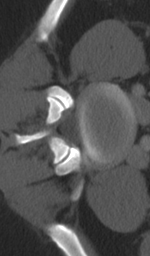
HRPSNR/SSIM

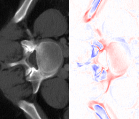
Bicubic34.21/0.9700

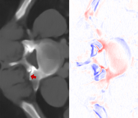
mDCSRN35.36/0.9770

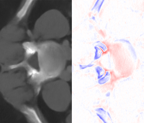
3D MDSR35.42/0.9777

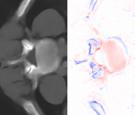
3D RDN36.17/0.9806

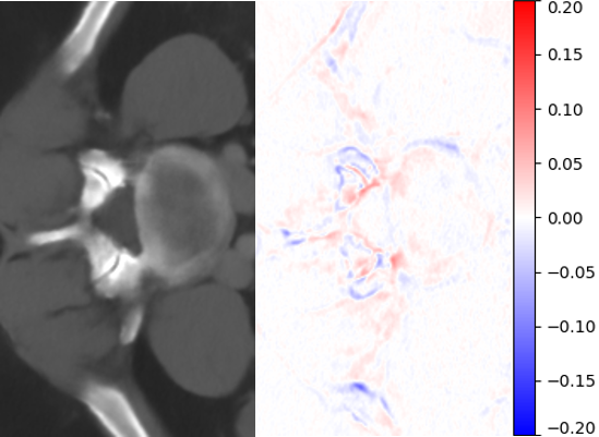
SAINT40.57/0.9888

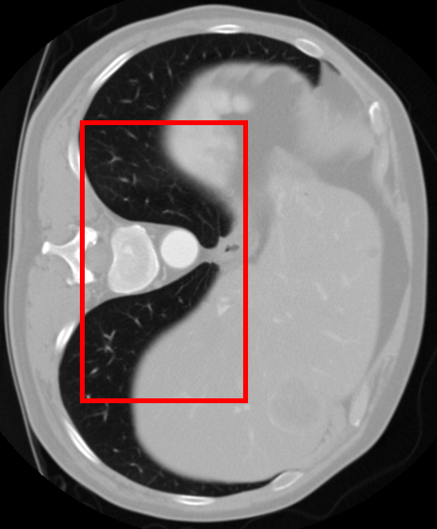
Ground Truth(b) x6

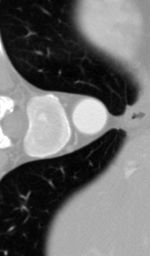
HRPSNR/SSIM

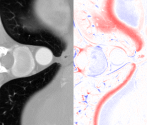
Bicubic30.36/0.9400

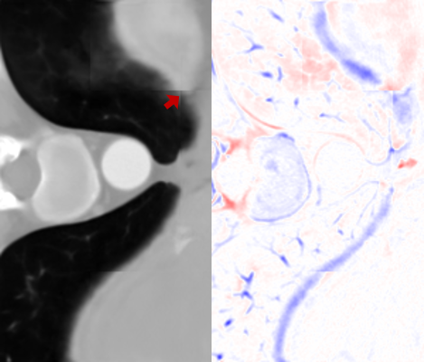
mDCSRN35.50/0.9711

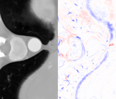
3D MDSR36.26/0.9750

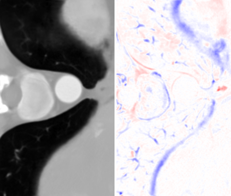
3D RDN35.46/0.9739

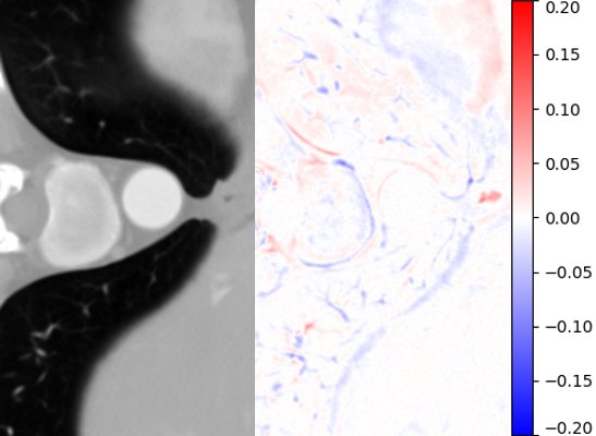
SAINT39.86/0.9863

Figure 7: Visual comparisons of different methods against SAINT. The difference maps are provided to the right of the results for better visualization. Images are best viewed when magnified.

4.2 Quantitative Evaluations

In this section, we evaluate the performance of our method and other SISR approaches. Quantitative comparisons are presented in Table 2. MDCSRN uses a DenseNet structure with batch normalization, which has been shown to adversely affect performance in super-resolution tasks [17, 27]. Furthermore, inference with 3D patches lead to observable artifacts where the patches are stitched together, as shown in the mDCSRN results in Fig. 7.

For liver, colon and hepatic vessels datasets, SAINT drastically outperforms the competing methods; however, the increase in performance is less significant with the kidney dataset. Generalizing over unseen dataset is a challenging problem for all data-driven methods, as factors such as acquisition machines, acquisition parameters, etc. subtly change the data distribution. Furthermore, quantitative measurements such as PSNR and SSIM do not always measure image quality well.

We visually inspect the results and find that SAINT generates richer detail when compared to other methods. It is evident in Fig. 7 that there is a least amount of structural artifacts remaining in the different images produced by SAINT. For more discussion on SAINT’s advantage in resolving the memory bottleneck and more slice interpolation results, please refer to the supplemental material section.

5 Conclusion

We propose a multi-stage 3D medical slice synthesis method called Spatially Aware Interpolation Network (SAINT). This method enables arbitrary upsampling ratios, alleviates memory constraint posed by competing 3D methods, and takes into consideration the changing voxel resolution of each 3D volume. We carefully evaluate our approach on four different CT datasets and find that SAINT produces consistent improvement in terms of visual quality and quantitative measures over other competing methods, despite that other methods are trained for dedicated upsampling ratios. SAINT is robust too, judging from its performance on the kidney dataset that is not involved in the training process. While we constrain the size of our network for fair comparisons with other methods, the multi-stage nature of SAINT allows for easy scaling in network size and performance improvement. Future work includes investigating the effect of SAINT on downstream analysis tasks, such as lesion segmentation, and improving performance in recovering minute details.

Appendix A Network Architecture

The proposed SAINT consists of AMI and RFN. For AMI, the model architecture for the feature learning stage is described in Section 4 and in [27] with more details. The model architecture for AMI’s filter generation stage is presented in Table 3. $N_{c}$ denotes the number of output channels, $C^{\prime}$ denotes the channel dimension of generated features $F^{LR}$. We use ‘K#-C#-S#-P#’ to denote the configuration of the convolution layers, where ‘K’, ‘C’, ‘S’ and ‘P’ stand for the kernel, channel, stride and padding size, respectively.

Name	$N_{c}$	Description
INPUT	$1$	Input FDM
CONV0	$32$	K3-C1-S1-P1
RELU
CONV1	$64$	K3-C64-S1-P1
RELU
CONV2	$64$	K3-C64-S1-P1
RELU
CONV3	$64$	K3-C64-S1-P1
RELU
CONV4	$C^{\prime}$	K3-C64-S1-P1

Table 3: Network architecture of AMI’s filter generation stage.

For RFN, we use RDN with five RDBs, four convolutional layers per RDB, and growth rate of sixteen. Additionally, for the first convolutional layer, RFN outputs thirty-two channels instead of sixty-four, which is the default hyperparameter in RDN and is used in AMI’s model construction. The upsampling module is a single convolutional layer, since the input and output have the same image height and width. We find that expanding RFN’s depth or width does not show improvement to the slice interpolation results quantitatively.

Appendix B Stitching Artifacts

Due to the high memory consumption of 3D volumetric data, CT volumes cannot be directly inferred through deep 3D CNN networks. In Section 4 we infer and compare only the central $256\times 256\times Z$ patch for all non-SAINT methods to reduce the memory requirement, with the exception of mDCSRN, which are inferred by the patch-based algorithm discussed in [4].

When an entire 3D volume needs to be super-resolved, all competing 3D CNN models need to use some form of patch-based algorithm that divides CT volumes into individual cubes to be inferred independently. However, such an approach introduces artifacts at the fringe, where the divided cubes are put back together. This is due to SISR models heavily employing padding to keep the same dimensionality throughout convolutions, i.e. for every convolutional layer with a filter size of $k$, the input tensor needs to be padded by $\lfloor\frac{k}{2}\rfloor$ for the output tensor to retain the same shape. For our implementation of the 3D RDN, there are fifty-two convolutional layers, which means the original input is padded by fifty-two voxels on each side, resulting in an overall padding size of $104\times 104\times 104$. Such a large padding size distorts the real data distribution, and adversely affects voxel prediction accuracy, especially at the fringe, of the divided cues. As a result, when the cubes are reassembled together to form the super-resolved volume, the boundaries between them are often inconsistent. We refer to the artifact caused by this inconsistency as the stitching artifact.

The patch-based algorithm discussed in [4] attempts to alleviate this problem by introducing overlaps of three voxels between the divided 3D cubes, effectively replacing the padding of three initial convolution layers with real voxel values. As we have shown in Fig. 7 and an enlarged version in Fig. 8, this still leads to noticeable stitching artifacts with a deep network. Theoretically, to completely eliminate such artifact for 3D RDN, the input tensor needs to be padded with at least fifty-two voxels on each side, which leads back to memory bottleneck and inefficiency. In comparison, since SAINT breaks down 3D SISR into separate stages of 2D SISR, it completely eliminates stitching artifacts, thus also allowing for larger network size to be used.

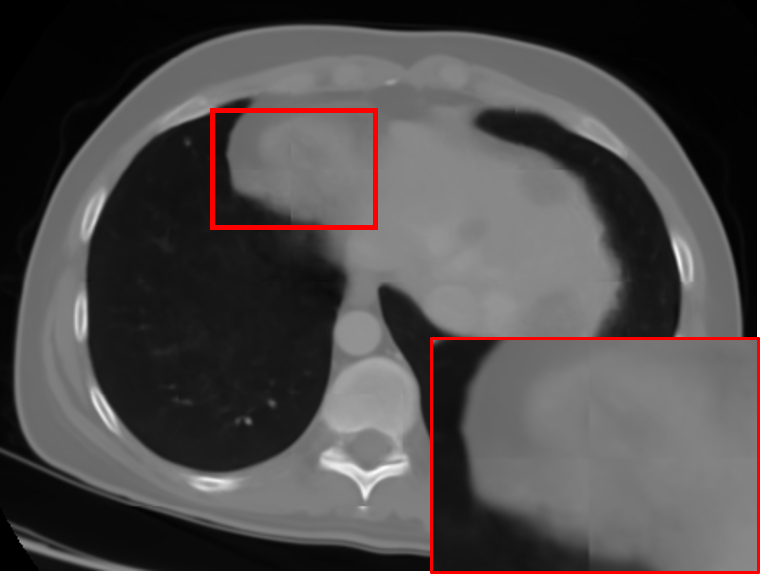
Figure 8: The stitching artifacts, following the procedure described in [4] with three voxel margin.

Appendix C Alternative RFN implementations

In this section, we showed the different implementations of RFN that we have experimented with.

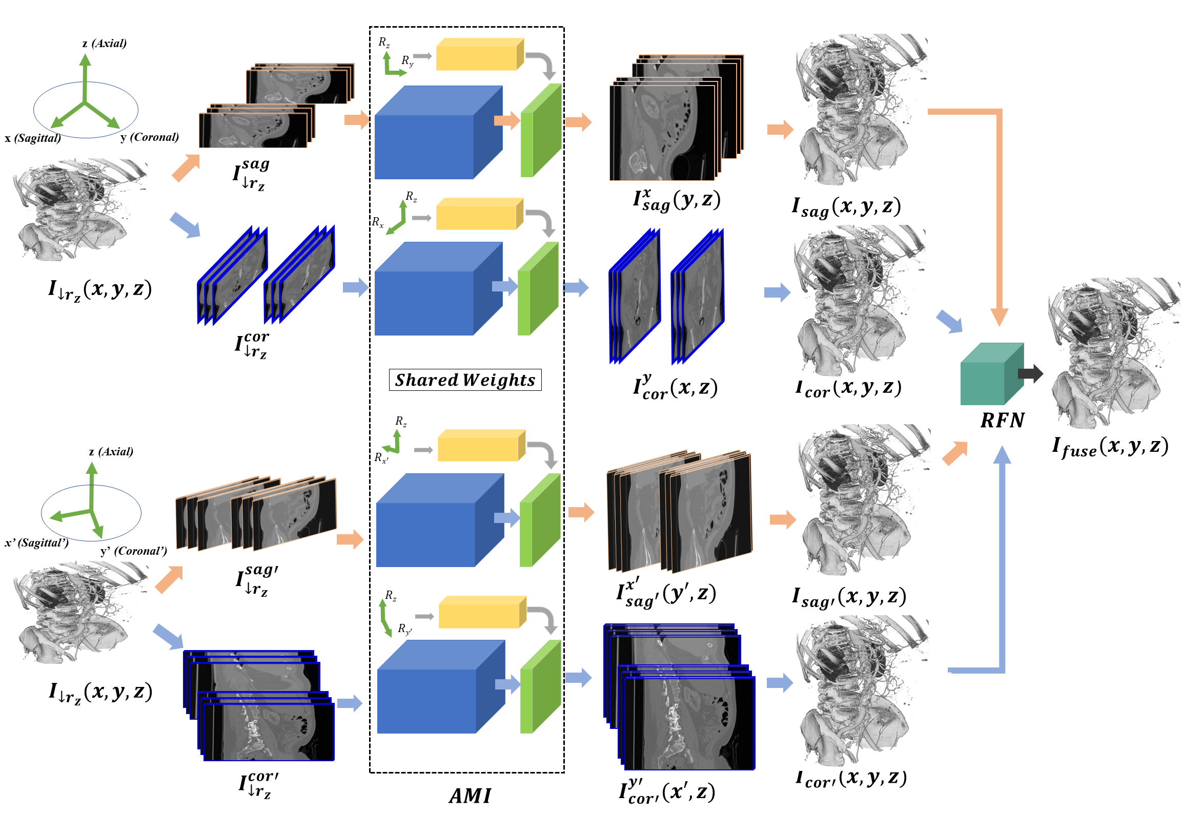
Figure 9: The augmented version of Spatially Aware Interpolation NeTwork (SAINT). Instead of using the sagittal and coronal views, the augmented SAINT also attempts to incorporate alternative views. For visualization purpose, the volumes are rendered in 3D based on their bone structures.

3D RFN Due to RFN’s lightweight and shallow network structure, it is memory-wise feasible to employ the patch-based algorithm for inference with enough margin on each side to eliminate the stitching artifacts. We implement a 3D version of RFN, where it uses 3D convolutional filters instead of 2D, to observe if that allows better modelling of the 3D context. As shown in Table 3, we do not see any observable difference quantitatively between 2D and 3D RFN’s results.

Four Views To axially interpolate a 3D volume, AMI first upsamples it from the coronal view and sagittal view, i.e. $I^{y}_{\downarrow r_{z}}(x,z)$ and $I^{x}_{\downarrow r_{z}}(y,z)$, and leaves RFN to improve consistency from the axial view $I^{z}(x,y)$. However, $I^{y}_{\downarrow r_{z}}(x,z)$ and $I^{x}_{\downarrow r_{z}}(y,z)$ are not the only two views in a 3D volume that can be used to super-resolve the $z$ axis. Technically, there are infinite number of views that include the $z$ axis in 3D. To this end, we perform an experiment to see if axially upsampling volumes from alternative views can improve performance.

As shown in Fig. 9, we experiment with an augmented version of SAINT, where AMI upsamples 2D images from four views, instead of just the sagittal and coronal views. In addition to $(x,z)$ and $(y,z)$, we define two additional axes $x^{\prime}$ and $y^{\prime}$, which are rotated from the $x$ and $y$ axes by 45°on the $(x,y)$ plane. Following similar procedures described in Section 3.1, we sample from volume $I_{\downarrow r_{z}}$ to obtain $I^{x^{\prime}}_{\downarrow r_{z}}(y^{\prime},z)$ and $I^{y^{\prime}}_{\downarrow r_{z}}(x^{\prime},z)$, of which we super-resolve with AMI. The super-resolved slices are reformatted into 3D volumes $I_{cor^{\prime}}(x^{\prime},y^{\prime},z)$ and $I_{sag^{\prime}}(x^{\prime},y^{\prime},z)$, and are passed to RFN with $I_{cor}$ and $I_{sag}$.

Scale	PSNR/SSIM	Parameters	Liver	Colon	Hepatic Vessels	Kidney
x4	AMI+$\mbox{RFN}^{2D}_{2View}$	2.92M	34.91/0.9603	34.19/0.9579	34.48/0.9630	35.79/0.9597
	AMI+$\mbox{RFN}^{3D}_{2View}$	2.92M	34.84/0.9602	34.21/0.9583	34.50/0.9631	35.44/0.9566
	AMI+$\mbox{RFN}^{2D}_{4View}$	2.92M	34.94/0.9611	34.29/0.9590	34.60/0.9639	35.56/0.9575
x6	AMI+$\mbox{RFN}^{2D}_{2View}$	2.92M	32.49/0.9395	31.48/0.9321	31.87/0.9404	33.22/0.9393
	AMI+$\mbox{RFN}^{3D}_{2View}$	2.92M	32.36/0.9390	31.51/0.9324	31.87/0.9404	32.92/0.9352
	AMI+$\mbox{RFN}^{2D}_{4View}$	2.92M	32.37/0.93890	31.52/0.9324	31.89/0.9404	32.92/0.9352

Table 4: Quantitative Comparison of different RFN implementations. The superscript on RFN describes whether RFN is implemented with 2D or 3D filters; the subscript describes whether RFN fuses volumes super-resolved from two views (sagittal and coronal) or four views (as described in C). The best results are in bold, and the second best results are underlined.

For RFN, $I_{avg}$ is the average of four volumes $I_{sag}$, $I_{cor}$, $I_{sag^{\prime}}$, $I_{cor^{\prime}}$, and $I^{z}_{fuse}$ becomes:

$$\begin{split}&I^{z}_{fuse}(x,y)=I^{z}_{avg}(x,y)\\ &+\mathcal{F_{\phi}}(I^{z}_{sag}(x,y),I^{z}_{cor}(x,y),I^{z}_{sag^{\prime}}(x,y),I^{z}_{cor^{\prime}}(x,y)).\end{split}$$ (12)

All loss functions and network structures remain the same. We found that the two additional planes only improve SAINT performance marginally.

Appendix D Effects of FDM on interpolation results

SAINT generates interpolated slices based on the input of FDM, which is dependent on the voxel spacing of specific slices (as shown in Algorithm 1). We believe that the incorporation of voxel spacing, especially the spacing between slices $R_{z}$, is important, as it is an indication of how much the details should shift between consecutive slices.

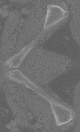
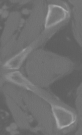
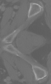
(a) Interpolated Results, $R_{z}=1mm$

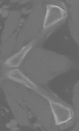
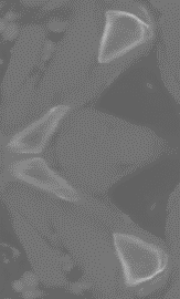
(b) Interpolated Results, $R_{z}=5mm$

Figure 11: Visual comparison of slice interpolation ($r_{z}=4$) with different voxel spacing input. Notice how the bone structures change faster for (a) as compared to (b), as the slices are supposed to be further apart according to the respective $R_{z}$.

To visually understand how changing voxel spacing values impact interpolation results from SAINT, we use AMI to super-resolve the same CT volume with different values of $R_{z}$, as shown in Fig. 11. We found that through the formulation of FDM, the interpolated slices produce details that change more rapidly if $R_{z}$ is high, and more slowly if $R_{z}$ is low.

References

- [1] S. Bakas et al. Advancing the cancer genome atlas glioma MRI collections with expert segmentation labels and radiomic features. Scientific data, 4, 2017.
- [2] H. Chen, Y. Zhang, Y. Chen, J. Zhang, W. Zhang, H. Sun, Y. Lv, P. Liao, J. Zhou, and G. Wang. Learn: Learned experts’ assessment-based reconstruction network for sparse-data ct. IEEE Transactions on Medical Imaging, 37(6):1333–1347, June 2018.
- [3] H. Chen, Y. Zhang, M. K. Kalra, F. Lin, Y. Chen, P. Liao, J. Zhou, and G. Wang. Low-dose ct with a residual encoder-decoder convolutional neural network. IEEE Transactions on Medical Imaging, 36(12):2524–2535, Dec 2017.
- [4] Y. Chen, F. Shi, A. G. Christodoulou, Z. Zhou, Y. Xie, and D. Li. Efficient and accurate MRI super-resolution using a generative adversarial network and 3d multi-level densely connected network. CoRR, abs/1803.01417, 2018.
- [5] C. Dong, C. C. Loy, K. He, and X. Tang. Image super-resolution using deep convolutional networks. CoRR, abs/1501.00092, 2015.
- [6] C. Dong, C. C. Loy, and X. Tang. Accelerating the super-resolution convolutional neural network. CoRR, abs/1608.00367, 2016.
- [7] I. J. Goodfellow, J. Pouget-Abadie, M. Mirza, B. Xu, D. Warde-Farley, S. Ozair, A. C. Courville, and Y. Bengio. Generative adversarial networks. CoRR, abs/1406.2661, 2014.
- [8] Y. Han and J. C. Ye. Framing u-net via deep convolutional framelets: Application to sparse-view CT. CoRR, abs/1708.08333, 2017.
- [9] N. Heller, N. Sathianathen, A. Kalapara, E. Walczak, K. Moore, H. Kaluzniak, J. Rosenberg, P. Blake, Z. Rengel, M. Oestreich, J. Dean, M. Tradewell, A. Shah, R. Tejpaul, Z. Edgerton, M. Peterson, S. Raza, S. Regmi, N. Papanikolopoulos, and C. Weight. The kits19 challenge data: 300 kidney tumor cases with clinical context, ct semantic segmentations, and surgical outcomes, 2019.
- [10] X. Hu, H. Mu, X. Zhang, Z. Wang, T. Tan, and J. Sun. Meta-sr: A magnification-arbitrary network for super-resolution. In The IEEE Conference on Computer Vision and Pattern Recognition (CVPR), June 2019.
- [11] G. Huang, Z. Liu, and K. Q. Weinberger. Densely connected convolutional networks. CoRR, abs/1608.06993, 2016.
- [12] Y. Jo, S. W. Oh, J. Kang, and S. J. Kim. Deep video super-resolution network using dynamic upsampling filters without explicit motion compensation. In 2018 IEEE/CVF Conference on Computer Vision and Pattern Recognition, pages 3224–3232, June 2018.
- [13] J. Kim, J. K. Lee, and K. M. Lee. Accurate image super-resolution using very deep convolutional networks. CoRR, abs/1511.04587, 2015.
- [14] J. Kim, J. K. Lee, and K. M. Lee. Deeply-recursive convolutional network for image super-resolution. In 2016 IEEE Conference on Computer Vision and Pattern Recognition, CVPR 2016, Las Vegas, NV, USA, June 27-30, 2016, pages 1637–1645, 2016.
- [15] C. Ledig, L. Theis, F. Huszar, J. Caballero, A. Cunningham, A. Acosta, A. P. Aitken, A. Tejani, J. Totz, Z. Wang, and W. Shi. Photo-realistic single image super-resolution using a generative adversarial network. In 2017 IEEE Conference on Computer Vision and Pattern Recognition, CVPR 2017, Honolulu, HI, USA, July 21-26, 2017, pages 105–114, 2017.
- [16] X. Li, H. Chen, X. Qi, Q. Dou, C. Fu, and P. Heng. H-denseunet: Hybrid densely connected unet for liver and tumor segmentation from ct volumes. IEEE Transactions on Medical Imaging, 37(12):2663–2674, Dec 2018.
- [17] B. Lim, S. Son, H. Kim, S. Nah, and K. M. Lee. Enhanced deep residual networks for single image super-resolution. CoRR, abs/1707.02921, 2017.
- [18] S. Liu, D. Xu, S. K. Zhou, T. Mertelmeier, J. Wicklein, A. K. Jerebko, S. Grbic, O. Pauly, W. Cai, and D. Comaniciu. 3d anisotropic hybrid network: Transferring convolutional features from 2d images to 3d anisotropic volumes. CoRR, abs/1711.08580, 2017.
- [19] B. H. Menze, A. Jakab, et al. The multimodal brain tumor image segmentation benchmark (BRATS). IEEE Trans. Med. Imaging, 34(10):1993–2024, 2015.
- [20] W. Shi, J. Caballero, F. Huszár, J. Totz, A. P. Aitken, R. Bishop, D. Rueckert, and Z. Wang. Real-time single image and video super-resolution using an efficient sub-pixel convolutional neural network, 2016.
- [21] A. L. Simpson, M. Antonelli, S. Bakas, M. Bilello, K. Farahani, B. van Ginneken, A. Kopp-Schneider, B. A. Landman, G. Litjens, B. Menze, O. Ronneberger, R. M. Summers, P. Bilic, P. F. Christ, R. K. G. Do, M. Gollub, J. Golia-Pernicka, S. H. Heckers, W. R. Jarnagin, M. K. McHugo, S. Napel, E. Vorontsov, L. Maier-Hein, and M. J. Cardoso. A large annotated medical image dataset for the development and evaluation of segmentation algorithms, 2019.
- [22] G. Wang, W. Li, S. Ourselin, and T. Vercauteren. Automatic brain tumor segmentation using cascaded anisotropic convolutional neural networks. Lecture Notes in Computer Science, page 178–190, 2018.
- [23] Y. Wang, Q. Teng, X. He, J. Feng, and T. Zhang. Ct-image super resolution using 3d convolutional neural network, 2018.
- [24] J. M. Wolterink, T. Leiner, M. A. Viergever, and I. Išgum. Generative adversarial networks for noise reduction in low-dose ct. IEEE Transactions on Medical Imaging, 36(12):2536–2545, Dec 2017.
- [25] T. Würfl, M. Hoffmann, V. Christlein, K. Breininger, Y. Huang, M. Unberath, and A. K. Maier. Deep learning computed tomography: Learning projection-domain weights from image domain in limited angle problems. IEEE Transactions on Medical Imaging, 37(6):1454–1463, June 2018.
- [26] K. Zhang, W. Zuo, S. Gu, and L. Zhang. Learning deep CNN denoiser prior for image restoration. In 2017 IEEE Conference on Computer Vision and Pattern Recognition, CVPR 2017, Honolulu, HI, USA, July 21-26, 2017, pages 2808–2817, 2017.
- [27] Y. Zhang, Y. Tian, Y. Kong, B. Zhong, and Y. Fu. Residual dense network for image super-resolution. CoRR, abs/1802.08797, 2018.
- [28] Z. Zhang, X. Liang, X. Dong, Y. Xie, and G. Cao. A sparse-view ct reconstruction method based on combination of densenet and deconvolution. IEEE Transactions on Medical Imaging, 37(6):1407–1417, June 2018.
- [29] X. Zheng, S. Ravishankar, Y. Long, and J. A. Fessler. PWLS-ULTRA: An Efficient Clustering and Learning-Based Approach for Low-Dose 3D CT Image Reconstruction. IEEE Transactions on Medical Imaging, 37(6):1498–1510, Jun 2018.