Experimental Detection of Non-local Correlations using a Local Measurement-Based Hierarchy on an NMR Quantum Processor

Abstract

The non-local nature of the correlations possessed by quantum systems may be revealed by experimental demonstrations of the violation of Bell-type inequalities. Recent work has placed bounds on the correlations that quantum systems can possess in an actual experiment. These bounds were limited to a composite quantum system comprising of a few lower-dimensional subsystems. In a more general approach, it has been shown that fewer body correlations can reveal the non-local nature of the correlations arising from a quantum mechanical description of nature. Such tests on the correlations can be transformed to a semi-definite program (SDP). This study reports the experimental implementation of a local measurement-based hierarchy on the nuclear magnetic resonance (NMR) hardware utilizing three nuclear spins as qubits. The protocol has been experimentally tested on genuinely entangled tripartite states such as W state, GHZ state and a few graph states. In all the cases, the experimentally measured correlations were used to formulate the SDP, using linear constraints on the entries of the moment matrix. We observed that for each genuinely entangled state, the SDP failed to find a semi-definite positive moment matrix consistent with the experimental data. This implies that the observed correlations can not arise from local measurements on a separable state and are hence non-local in nature, and also confirms that the states being tested are indeed entangled.

I Introduction

It is well established that quantum computation has a computational advantage over its classical counterpart and the main resources utilized for quantum computation are superposition, entanglement and other quantum features like contextuality Nielsen and Chuang (2000). Entanglement plays a key role in several quantum computational tasks, including quantum teleportation (Bennett et al., 1993), quantum super dense coding (Bennett and Wiesner, 1992), measurement-based quantum computation (Briegel et al., 2009) and quantum key distribution schemes (Ekert, 1991; Barrett et al., 2005; Acín et al., 2006). Creating entangled states in an experiment and certifying the presence of entanglement in such states is hence of utmost importance (Gühne and Tóth, 2009; Horodecki et al., 2009) from a practical as well as the foundational points of view. Most of the known entanglement detection schemes rely on experimental quantum state reconstruction (Horodecki et al., 2009), however it has been shown that quantum state reconstruction is not cost-effective with respect to experimental and computational resources (Häffner et al., 2005). Furthermore, the detection of entanglement of a known quantum state is computationally a hard problem (Brandão and Christandl, 2012) and scales exponentially with the number of qubits. Methods to detect entanglement include the use of violation of Bell-type inequalities (Huber et al., 2011; Jungnitsch et al., 2011), entanglement witnesses (Lewenstein et al., 2000; Gühne et al., 2003), expectation values of the Pauli operators (Zhao et al., 2013; Miranowicz et al., 2014) as well as dynamical learning techniques (Behrman et al., 2008). Although a number of schemes exist for entanglement detection, most of them lack generality and therefore more research is required in this direction.

A promising direction of research on entanglement is to experimentally observe the violation of Bell-type inequalities (Bell and Aspect, 2004; Bell, 1964; Clauser et al., 1969), and such inequalities have recently been proposed as a general method for certifying the non-local nature of the experimentally observed correlations in a device-independent manner (Navascués et al., 2007; Pironio et al., 2010; Baccari et al., 2017). Consider a joint probability distribution $P_{\alpha\beta}$. The question addressed in Ref.(Navascués et al., 2007) is that can there be a quantum description of $P_{\alpha\beta}$ i.e. can one have a quantum state $\rho$, acting on the joint Hilbert space $\mathcal{H}_{A}\otimes\mathcal{H}_{B}$, and the local measurement operators $E_{\alpha}=\tilde{E}_{\alpha}\otimes I$ and $E_{\beta}=I\otimes\tilde{E}_{\beta}$ such that

$$P_{\alpha\beta}=Tr(E_{\alpha}E_{\beta}.\rho)$$ (1)

where $\tilde{E}_{\alpha}$ and $\tilde{E}_{\beta}$ are local projection operators. This can be used to design a test for the detection of non-locality from the actual probability distribution $P_{\alpha\beta}$. In general, one may need to search over all physical $\rho$ and projection operators $E_{\mu}$ which makes the problem computationally hard. A few attempts have been made to solve this problem, including finding the maximum violation of the Clauser Horne Shimony Holt (CHSH) inequality (Clauser et al., 1969) by a quantum description (Cirel’son, 1980). Notable work has been done by Landau (Landau, 1988) and Wehner (Wehner, 2006), where they have showed that the test of whether the experimental correlations arise from quantum mechanical description of nature or not, can be transformed to a semi-definite program (SDP). Solving such an SDP can reveal the local or non-local nature of the observed correlations.

In this article we describe the details of the experimental implementation of a local measurement-based hierarchy to certify the non-local correlations arising from local measurements (Navascués et al., 2007; Pironio et al., 2010; Baccari et al., 2017) on a system of three NMR qubits. The motivation of the investigation is to experimentally implement a non-local correlation and thereby devise an entanglement detection protocol which can readily be generalized to higher numbers of qubits as well as to multi-dimensional quantum systems. We experimentally generate high fidelity genuinely entangled multipartite states using three NMR qubits. In order to experimentally test the NPA hierarchy the desired correlators were measured with high precision. In our experimental investigations, these correlators are the three-qubit Pauli observables. The expectation values of the Pauli observables were used to formulate the moment matrix of SDP. Our earlier developed techniques (Singh et al., 2016, 2018a, 2018b) were utilized to find the expectation values of the desired correlators, in a given state of the ensemble. SDP optimization failure in finding a positive moment matrix is an indication that the correlations encoded in the observed correlators are non-local in nature and hence the state under investigation is entangled. Experimental verification was done by formulating the SDP by directly computing the correlators from the tomographed state. Further, we note here that the subsystems involved in our experiments reside on the same molecule and therefore strictly speaking, it is not possible to achieve a space-like separation between the events occurring in the different subsystem spaces. Therefore, the term “local” here pertains to subsystems and non-local implies something that goes across subsystems.

The paper is organized as follows: Sec.-II introduces the main features of local measurement based hierarchy and the formulation of the corresponding SDP, while Sec.-II.1 outlines the modified hierarchy obtained by introducing a relaxation due to commuting local measurements (Navascués et al., 2007). Sec.-III details the SDP formulation, and the experimental implementation using NMR. Sec.-IV contains a few concluding remarks.

II Revisiting Local Measurement-Based Hierarchy

To discuss the entanglement detection scenario, consider an N-partite quantum state $\rho_{N}$, which is shared by N observers. The joint probability distribution can be considered to arise from the local measurements on a separable state $\rho_{N}$. As the state $\rho_{N}$ is shared amongst $N$ parties, each of which can perform ‘$m$’ different measurements, each such measurement can result in ‘$d$’ different outcomes. Measurement by the $i^{\mathrm{th}}$ party is represented by observables $M_{x_{i}}^{a_{i}}$ with $x_{i}\in\{0,...,m-1\}$ being the measurement choice and $a_{i}\in\{0,...,d-1\}$ being the corresponding outcome. By observing the statistics generated by measuring all possible $M_{x_{i}}^{a_{i}}$, one may write the empirical values for the conditional probability distributions as

$$p(a_{1},...,a_{N}|x_{1},...,x_{N})=Tr(M_{x_{1}}^{a_{1}}\otimes...\otimes M_{x_{N}}^{a_{N}}\rho_{N})$$ (2)

The correlations observed by measuring $M_{x_{i}}^{a_{i}}$ locally, get encoded in the conditional probability distributions having the form of Eq.(2). Similar expressions can be written for the reduced state probability distributions which may arise from local measurements on a reduced system.

$$p(a_{i_{1}},...,a_{i_{k}}|x_{i_{1}},...,x_{i_{k}})=Tr(M_{x_{i_{1}}}^{a_{i_{1}}}\otimes...\otimes M_{x_{i_{k}}}^{a_{i_{k}}}\rho_{i_{1}.....i_{k}})$$

where $0\leq i_{1}<...<i_{k}<N$,  $1\leq k<N$ and $\rho_{i_{1}.....i_{k}}$ is the reduced density matrix obtained from $\rho_{N}$. While dealing with dichotomic measurements on qubits, it is useful to introduce the concept of correlators and their expectation values as follows

$$\langle M_{x_{i_{1}}}^{(i_{1})}...M_{x_{i_{k}}}^{(i_{k})}\rangle =$$

$$\sum_{a_{i_{1}},...a_{i_{k}}} (-1) {}^{\sum_{l=1}^{k}a_{i_{l}}}p(a_{i_{1}},...a_{i_{k}}|x_{i_{1}},...x_{i_{k}})$$ (3)

The index $k$ here dictates the order of the correlator while $0\leq i_{1}<...<i_{k}<N$ with $x_{i_{j}}\in\{0,m-1\}$ and $1\leq k\leq N$. One may note that for dichotomic measurements it is convenient to introduce $M_{x_{i}}^{(i)}=M_{x_{i}}^{(1)}-M_{x_{i}}^{(0)}$ and the $\langle M_{x_{i_{1}}}^{(i_{1})}...M_{x_{i_{k}}}^{(i_{k})}\rangle=Tr(M_{x_{i_{1}}}^{(i_{1})}\otimes...\otimes M_{x_{i_{k}}}^{(i_{k})}\rho_{i_{1},...,i_{k}})$. For $k=2$ the correlator will be of second order having the form $\langle M_{x_{i_{1}}}^{(i_{1})}M_{x_{i_{2}}}^{(i_{2})}\rangle$ while for $k=N$ one can have the full body correlator. It will be seen later that these correlators in the simplest case turn out to be multi-qubit Pauli operators. For example, using Eq.(II), for a two-qubit system the $\langle M_{3}^{(1)}M_{3}^{(2)}\rangle=\langle\sigma^{(1)}_{z}\otimes\sigma^{(2)}_{z}\rangle=(-1)^{0+0}p(0,0|\sigma^{(1)}_{z},\sigma^{(2)}_{z})+(-1)^{0+1}p(0,1|\sigma^{(1)}_{z},\sigma^{(2)}_{z})+(-1)^{1+0}p(1,0|\sigma^{(1)}_{z},\sigma^{(2)}_{z})+(-1)^{1+1}p(1,1|\sigma^{(1)}_{z},\sigma^{(2)}_{z})$ which implies that the expectation value of a correlator is the sum of the products of various outcome probabilities with the respective eigenvalues.

The method to detect entanglement, introduced in Ref.(Baccari et al., 2017), assumes that:

• Local measurements on a separable state $\rho_{N}$ can produce local correlations exhibiting local models.

• Local commuting measurements on a quantum state can reveal all the local correlations.

• A positive moment matrix can be defined using correlations produced by commuting local measurements, considering the constraints due to commutation of measurements.

The main assumption above can be explained as follows. Consider that state $\rho_{N}$ is a separable state and thus can be written as $\rho_{N}=\sum_{\lambda}p_{\lambda}\otimes_{i}\rho_{\lambda}^{i}$. One can write the conditional probabilities produced by local measurements on such a separable state as

$$p(a_{1},...,a_{N}|x_{1},...,x_{N}) = \sum_{\lambda}p_{\lambda}Tr(\otimes_{i}M_{x_{i}}^{a_{i}}\otimes_{i}\rho_{\lambda}^{i})$$ (4)

$$= \sum_{\lambda}p_{\lambda}\prod_{i}^{N}p(a_{i}|x_{i},\lambda)$$

As in Bell nonlocality, the probability distributions exhibiting the above form are local in nature and they do not violate any Bell-type inequality. Conversely, if one can not write an observed distribution in the above form, then the distribution is non-local. Hence whenever the conditional probability distributions given by Eq.(2) are non-local, i.e. do not exhibit the form of Eq.(4), the state under consideration possesses non-local correlations and is thus entangled.

In order to define the SDP for the Navascués-Pironio-Acín (NPA) hierarchy based on local measurements, consider the projectors $E_{\nu}$ and $E_{\mu}$, corresponding to outcomes of a measurement $M$, labeled by $\nu$ and $\mu$. Here $M$ may or may not be a projective measurement. These projectors satisfy the following constraints:

1. are orthogonal i.e. $E_{\nu}E_{\mu}=0$ for $\nu$, $\mu\in$ M, $\mu\neq\nu$.

2. sum to identity i.e. $\sum_{\mu\in M}E_{\mu}=I$.

3. obey $E_{\mu}^{2}=E_{\mu}^{\dagger}=E_{\mu}$.

4. obey the commutation rule (for projectors on subsystems A and B) as $[E_{\alpha},E_{\beta}]=0$.

It was assumed in Ref. (Navascués et al., 2007) that such a $\rho$ exists which satisfies Eq.(1) and the projector constraints. It was noted that by taking products of projection operators $E_{\mu}$ and linear superpositions of such products, one may define new operators which may neither be projectors anymore nor be Hermitian. Let $S=\{S_{1},S_{2},....,S_{n}\}$ be a set of $n$ such operators. There exists an $n\times n$ matrix associated with every such set $S$ and defined as

$$\Gamma_{ij}=Tr(S_{i}^{\dagger}S_{j}\rho)$$ (5)

$\Gamma$ is Hermitian and satisfies

$$\sum_{i,j}c_{ij}S_{i}^{\dagger}S_{j}=0\;\;\;\Rightarrow\;\;\;\sum_{i,j}c_{ij}\Gamma_{ij}=0$$ (6)

$$\sum_{i,j}c_{ij}S_{i}^{\dagger}S_{j}=\sum_{\alpha,\beta}d_{\alpha\beta}E_{\alpha}E_{\beta}\;\Rightarrow\;\sum_{i,j}c_{ij}\Gamma_{ij}=\sum_{\alpha,\beta}d_{\alpha\beta}P_{\alpha\beta}$$ (7)

Further, it can be proved that $\Gamma$ is positive semi-definite i.e. $\Gamma\geq 0$ (Navascués et al., 2007). Hence, if a joint probability distribution $P_{\alpha\beta}$ has a quantum description i.e. there exists a state $\rho$ and local measurement operators satisfying Eq.(1) and projector constraints respectively, then finding such a state is equivalent to finding the matrix $\Gamma\geq 0$ satisfying linear constraints similar to Eq. (6) and Eq. (7). This amounts to solving an SDP problem.

II.1 Modified NPA hierarchy

Having discussed the main features of the NPA hierarchy(Navascués et al., 2007), we now turn to the method to detect non-local correlations. Consider a set $O=\{O_{i}\}$ with $1\leq i\leq k$ and $O_{i}$ being some product of the measurement operators $\{\rm M_{x_{i}}^{a_{i}}\}$ or their linear combinations. One can associate a $k\times k$ matrix with $O$ defined by Eq.(5) as $\Gamma_{ij}=$Tr$(O_{i}^{\dagger}O_{j}.\rho_{N})$. For a given choice of measurements on a separable state: (a) $\Gamma$ will be a positive semi-definite matrix, (b) matrix elements of $\Gamma$ satisfy the linear constraints similar to Eq.(6)-(7), (c) some of the matrix elements of $\Gamma$ can be obtained by experimentally measuring the probability distribution and (d) some of the $\Gamma$ matrix entries correspond to unobservables, as entries of the moment matrix are expectation values of observables, which necessarily need to be represented by Hermitian operators. However, in case the element of the moment matrix arises from a non-Hermitian operator, the respective expectation value is unobservable and thus enters the moment matrix as a parameter to be optimized in SDP.

Keeping these facts in mind, one can design a hierarchy-based test to see if a given set of correlations can arise from an actual quantum realization by performing local measurements on a separable state. One can define a set $O_{\nu}$ consisting of products of ‘$\nu$’ local measurement operators or linear superpositions of such products. Once $O_{\nu}$ is defined, one can look for associated $\Gamma\geq 0$ satisfying constraints similar to Eq.(6)-(7) to see if a given set of correlations can arise from actual local measurements on a separable state. If no solution is obtained to such an SDP, then this would imply that the given set of correlations cannot arise by local measurements on a separable quantum state and hence the correlations are non-local. One can always find a stricter set of constraints by increasing the value of $\nu$ i.e. testing the nature of correlations at the next level of the hierarchy.

In the experimental demonstration, as suggested in Ref.(Baccari et al., 2017), a set of commutating measurements have been used to formulate the SDP i.e. an additional constraint is introduced on the entries of $\Gamma$ such that local measurements also commutate. This additional constraint considerably reduces the original computationally-hard problem (Baccari et al., 2017). All the ideas developed till now can be understood with an example. Consider $N=2$, two dichotomic measurements per party at the hierarchy level $\nu=2$. Let the measurements be labeled as $A_{x}$ and $B_{y}$ with $x,y\in[0,1]$. Set of operators is $O_{2}=\{I,A_{0},A_{1},B_{0},B_{1},A_{0}A_{1},A_{0}B_{0},A_{0}B_{1},A_{1}B_{0},A_{1}B_{1},B_{0}B_{1}\}$. One can write the corresponding moment matrix $\Gamma$ as (Baccari et al., 2017)

$$\Gamma=\left(\begin{array}[]{lllllllllll}1&{\color[rgb]{1,0,0}\langle A_{0}\rangle}&{\color[rgb]{0,0,0}\langle A_{1}\rangle}&{\color[rgb]{0,0,1}\langle B_{0}\rangle}&{\color[rgb]{0,0,0}\langle B_{1}\rangle}&\color[rgb]{1,0.84,0}{v_{1}}&\color[rgb]{0,0.58,0}{\langle A_{0}B_{0}\rangle}&{\color[rgb]{.75,0,.25}\langle A_{0}B_{1}\rangle}&{\color[rgb]{1,.5,0}\langle A_{1}B_{0}\rangle}&{\color[rgb]{0,0,0}\langle A_{1}B_{1}\rangle}&{\color[rgb]{0.49,0.62,0.75}v_{2}}\\ {\color[rgb]{1,0,0}\langle A_{0}\rangle}&1&\color[rgb]{1,0.84,0}{v_{1}}&\color[rgb]{0,0.58,0}{\langle A_{0}B_{0}\rangle}&{\color[rgb]{.75,0,.25}\langle A_{0}B_{1}\rangle}&{\color[rgb]{0,0,0}\langle A_{1}\rangle}&{\color[rgb]{0,0,1}\langle B_{0}\rangle}&{\color[rgb]{0,0,0}\langle B_{1}\rangle}&\color[rgb]{0.55,0,0}{v_{3}}&{\color[rgb]{0,1,0}v_{4}}&{\color[rgb]{1,0,1}v_{5}}\\ {\color[rgb]{0,0,0}\langle A_{1}\rangle}&\color[rgb]{1,0.84,0}{v_{1}^{\ast}}&1&{\color[rgb]{1,.5,0}\langle A_{1}B_{0}\rangle}&{\color[rgb]{0,0,0}\langle A_{1}B_{1}\rangle}&{\color[rgb]{1,0,0}v_{6}}&\color[rgb]{0.55,0,0}{v_{3}^{\ast}}&{\color[rgb]{0,1,0}v_{4}^{\ast}}&{\color[rgb]{0,0,1}\langle B_{0}\rangle}&{\color[rgb]{0,0,0}\langle B_{1}\rangle}&\color[rgb]{0.55,0.55,0}{v_{7}}\\ {\color[rgb]{0,0,1}\langle B_{0}\rangle}&\color[rgb]{0,0.58,0}{\langle A_{0}B_{0}\rangle}&{\color[rgb]{1,.5,0}\langle A_{1}B_{0}\rangle}&1&{\color[rgb]{0.49,0.62,0.75}v_{2}}&\color[rgb]{0.55,0,0}{v_{3}}&{\color[rgb]{1,0,0}\langle A_{0}\rangle}&{\color[rgb]{1,0,1}v_{5}}&{\color[rgb]{0,0,0}\langle A_{1}\rangle}&\color[rgb]{0.55,0.55,0}{v_{7}}&{\color[rgb]{0,0,0}\langle B_{1}\rangle}\\ {\color[rgb]{0,0,0}\langle B_{1}\rangle}&{\color[rgb]{.75,0,.25}\langle A_{0}B_{1}\rangle}&{\color[rgb]{0,0,0}\langle A_{1}B_{1}\rangle}&{\color[rgb]{0.49,0.62,0.75}v_{2}^{\ast}}&1&{\color[rgb]{0,1,0}v_{4}}&{\color[rgb]{1,0,1}v_{5}^{\ast}}&{\color[rgb]{1,0,0}\langle A_{0}\rangle}&\color[rgb]{0.55,0.55,0}{v_{7}^{\ast}}&{\color[rgb]{0,0,0}\langle A_{1}\rangle}&{\color[rgb]{0,0,1}v_{8}}\\ \color[rgb]{1,0.84,0}{v_{1}^{\ast}}&{\color[rgb]{0,0,0}\langle A_{1}\rangle}&{\color[rgb]{1,0,0}v_{6}^{\ast}}&\color[rgb]{0.55,0,0}{v_{3}^{\ast}}&{\color[rgb]{0,1,0}v_{4}^{\ast}}&1&{\color[rgb]{1,.5,0}\langle A_{1}B_{0}\rangle}&{\color[rgb]{0,0,0}\langle A_{1}B_{1}\rangle}&{\color[rgb]{0.24,0.7,0.44}v_{9}}&{\color[rgb]{.75,0,.25}v_{10}}&\color[rgb]{0,1,1}{v_{11}}\\ \color[rgb]{0,0.58,0}{\langle A_{0}B_{0}\rangle}&{\color[rgb]{0,0,1}\langle B_{0}\rangle}&\color[rgb]{0.55,0,0}{v_{3}}&{\color[rgb]{1,0,0}\langle A_{0}\rangle}&{\color[rgb]{1,0,1}v_{5}}&{\color[rgb]{1,.5,0}\langle A_{1}B_{0}\rangle}&1&{\color[rgb]{0.49,0.62,0.75}v_{2}}&\color[rgb]{1,0.84,0}{v_{1}}&\color[rgb]{0,1,1}{v_{12}}&{\color[rgb]{.75,0,.25}\langle A_{0}B_{1}\rangle}\\ {\color[rgb]{.75,0,.25}\langle A_{0}B_{1}\rangle}&{\color[rgb]{0,0,0}\langle B_{1}\rangle}&{\color[rgb]{0,1,0}v_{4}}&{\color[rgb]{1,0,1}v_{5}^{\ast}}&{\color[rgb]{1,0,0}\langle A_{0}\rangle}&{\color[rgb]{0,0,0}\langle A_{1}B_{1}\rangle}&{\color[rgb]{0.49,0.62,0.75}v_{2}\ast}&1&\color[rgb]{0,1,1}{v_{13}}&\color[rgb]{1,0.84,0}{v_{1}}&\color[rgb]{0,0.58,0}{v_{14}}\\ {\color[rgb]{1,.5,0}\langle A_{1}B_{0}\rangle}&\color[rgb]{0.55,0,0}{v_{3}^{\ast}}&{\color[rgb]{0,0,1}\langle B_{0}\rangle}&{\color[rgb]{0,0,0}\langle A_{1}\rangle}&\color[rgb]{0.55,0.55,0}{v_{7}}&{\color[rgb]{0.24,0.7,0.44}v_{9}^{\ast}}&\color[rgb]{1,0.84,0}{v_{1}^{\ast}}&\color[rgb]{0,1,1}{v_{13}^{\ast}}&1&{\color[rgb]{0.49,0.62,0.75}v_{2}}&{\color[rgb]{0,0,0}\langle A_{1}B_{1}\rangle}\\ {\color[rgb]{0,0,0}\langle A_{1}B_{1}\rangle}&{\color[rgb]{0,1,0}v_{4}^{\ast}}&{\color[rgb]{0,0,0}\langle B_{1}\rangle}&\color[rgb]{0.55,0.55,0}{v_{7}^{\ast}}&{\color[rgb]{0,0,0}\langle A_{1}\rangle}&{\color[rgb]{.75,0,.25}v_{10}^{\ast}}&\color[rgb]{0,1,1}{v_{12}^{\ast}}&\color[rgb]{1,0.84,0}{v_{1}^{\ast}}&{\color[rgb]{0.49,0.62,0.75}v_{2}\ast}&1&{\color[rgb]{1,.5,0}v_{15}}\\ {\color[rgb]{0.49,0.62,0.75}v_{2}^{\ast}}&{\color[rgb]{1,0,1}v_{5}\ast}&\color[rgb]{0.55,0.55,0}{v_{7}^{\ast}}&{\color[rgb]{0,0,0}\langle B_{1}\rangle}&{\color[rgb]{0,0,1}v_{8}^{\ast}}&\color[rgb]{0,1,1}{v_{11}^{\ast}}&{\color[rgb]{.75,0,.25}\langle A_{0}B_{1}\rangle}&\color[rgb]{0,0.58,0}{v_{14}^{\ast}}&{\color[rgb]{0,0,0}\langle A_{1}B_{1}\rangle}&{\color[rgb]{1,.5,0}v_{15}^{\ast}}&1\end{array}\right)$$ (8)

while following are the unassigned variables

$\begin{array}[]{lll}v_{1}=\langle A_{0}A_{1}\rangle,&v_{2}=\langle B_{0}B_{1}\rangle,&v_{3}=\langle A_{0}A_{1}B_{0}\rangle,\\ v_{4}=\langle A_{0}A_{1}B_{1}\rangle,&v_{5}=\langle A_{0}B_{0}B_{1}\rangle,&v_{6}=\langle A_{1}A_{0}A_{1}\rangle,\\ v_{7}=\langle A_{1}B_{0}B_{1}\rangle,&v_{8}=\langle B_{1}B_{0}B_{1}\rangle,&v_{9}=\langle A_{1}A_{0}A_{1}B_{0}\rangle,\\ v_{10}=\langle A_{1}A_{0}A_{1}B_{1}\rangle,&v_{11}=\langle A_{1}A_{0}B_{0}B_{1}\rangle,&v_{12}=\langle A_{0}A_{1}B_{0}B_{1}\rangle,\\ v_{13}=\langle A_{0}A_{1}B_{1}B_{0}\rangle,&v_{14}=\langle A_{0}B_{1}B_{0}B_{1}\rangle,&v_{15}=\langle A_{1}B_{1}B_{0}B_{1}\rangle.\end{array}$

We note that by introducing local measurements commutativity i.e. $[A_{0},A_{1}]=[B_{0},B_{1}]=0$ the matrix elements, of the $\Gamma$ matrix given by Eq.(8) were simplified. Specifically, the following reduction in the number of variables can be noticed : $v_{i}=v_{i}^{\ast}$ for $i\in[1,15]$ and $v_{6}=\langle A_{0}\rangle$, $v_{8}=\langle B_{0}\rangle$, $v_{9}=v_{14}=\langle A_{0}B_{0}\rangle$, $v_{10}=\langle A_{0}B_{1}\rangle$, $v_{15}=\langle A_{1}B_{0}\rangle$ and also $v_{11}=v_{12}=v_{13}$. For a visual representation, the variables that become identical because of the commutativity constraints are represented by the same color in Eq.(8) (Baccari et al., 2017). The generated SDP will check if the set of observed correlations $\{\langle A_{x}\rangle,\langle B_{y}\rangle,\langle A_{x}B_{y}\rangle\}$ are local. This can be achieved by substituting the experimental values of the correlators in the $\Gamma$ matrix and leaving the unobservables as variables. The SDP will optimize over such variables to see if a given set of correlations are local or non-local. It has been shown (Navascués et al., 2008; Pironio et al., 2010) that this method converges i.e. if a given set of correlations are non-local then the SDP will fail at a finite number of steps $\nu$.

III Detection of Tripartite Non-Local Correlations

A three-qubit system was used to experimentally demonstrate the detection of correlations which can not arise from local measurements on a separable state. It has been shown Dür et al. (2000) that a genuine three-qubit system can be entangled in two inequivalent ways. The CHSH scenario (Clauser et al., 1969) deals with the (2,2,2) case i.e. $N=2$, $m=2$ and $d=2$. Any correlation violating the CHSH inequality exhibits non-local nature in the sense that, in principle one cannot write a local hidden variable theory which can reproduce the observed statistics. In the current experimental study, the scenarios are (3,2,2) and (3,3,2) i.e. three parties with two (or three) dichotomic observables per party. The measurements of three parties are labeled as $A_{x}$ , $B_{y}$ and $C_{z}$ respectively with measurement labels $x,y,z\in[0,1]$ in the (3,2,2) scenario while $x,y,z\in[0,1,2]$ in the (3,3,2) scenario. One can construct set $O_{2}$ for three parties, the way it was done in the previous section for $N=2$. As detailed in Ref. (Baccari et al., 2017), to detect non-local correlations arising from the W state, one needs to perform local measurements $M_{0}^{(i)}=\sigma_{x}$ and $M_{1}^{(i)}=\sigma_{z}$ for all three parties for the observables entering the moment matrix associated with $O_{2}$ defined above. Here $\sigma_{x/y/z}$ are the spin-1/2 Pauli operators. For GHZ type states, the measurements to generate the statistics were chosen as $M_{0}^{(i)}=\sigma_{x}$ and $M_{1}^{(i)}=\frac{1}{\sqrt{2}}(\sigma_{z}+\sigma_{x})$. A full body correlator is also introduced while detecting non-local correlations generated by the GHZ state as such states are not suitable for detection of non-local correlation using fewer body correlators (Baccari et al., 2017). Further, for graph states $M_{0}^{(i)}=\sigma_{x}$, $M_{1}^{(i)}=\sigma_{z}$ and $M_{2}^{(i)}=\frac{1}{\sqrt{2}}(\sigma_{z}+\sigma_{x})$ were chosen as measurements.

III.1 NMR implementation of the detection scheme

A system of three NMR qubits was chosen to experimentally demonstrate the detection of non-local correlations. The system was initialized in either of the W, GHZ, linear or loop graph states (see Ref.(Hein et al., 2004) for the definition of graph states). The quantum circuits as well as NMR pulse sequence to prepare W and GHZ states are detailed in Ref.(Singh et al., 2016, 2018a, 2018b). A compact quantum circuit to prepare the linear as well as loop graph state is shown in Fig.1. The third controlled-Z gate in Fig.1 (enclosed by a red dotted box) does not act while preparing the linear graph state.

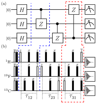
Figure 1: (a) Quantum circuit to prepare linear and loop graph states on a three-qubit quantum processor. The third controlled-Z gate, enclosed in red dashed line, acts only if the circuit is being used to prepare the loop graph state. (b) The NMR pulse sequence for the quantum circuit shown in (a). The unfilled rectangles denote $\frac{\pi}{2}$ spin-selective RF pulses while the filled black rectangles denote $\pi$ RF pulses. The phase of each pulse is written above the respective pulse and a bar over the phase represents negative phase. Delays are given by $\tau_{ij}=1/(8J_{ij})$; $i,j$ are the qubit labels and $J$ denotes the scalar coupling constant.

The protocol to test the non-locality present in the experimentally observed expectation values of the correlators, for a given state, is as follows:

• The system was initialized in one of the genuine tripartite pure states, either W, GHZ or graph states.

• It was assumed that the correlations observed from local measurements on such states will fail the SDP, formulated in Sec.-II, at the second level of the modified NPA hierarchy.

• At the second level ($\nu=2$) of the hierarchy, the expectation values of all the correlators were measured experimentally in the state under investigation.

• Once all the observables of the moment matrix $\Gamma$ Eq.(5) were measured experimentally, they were fed into the matrix $\Gamma$. The remaining unobservable entries of the moment matrix were left as variables to be optimized via SDP, to achieve $\Gamma\geq 0$ under linear constraints similar to Eq.(6)-(7) as well as the commutativity relaxation constraints i.e. $[A_{0},A_{1}]=[B_{0},B_{1}]=[C_{0},C_{1}]=0$ in (3,2,2) scenario.

• The above formulated SDP was solved by modifying the codes, available at Baccari (2016), for the (3,2,2) or (3,3,2) scenario.

III.2 NMR experimental set-up and system initialization

For the experimental realization,¹³C-labeled diethylflouromalonate sample dissolved in acetone-D6 is used, with three spin-$\frac{1}{2}$ nuclei i.e. ¹H, ¹⁹F and ¹³C encoding the qubit 1, qubit 2 and qubit 3, respectively. In such a scenario, the free Hamiltonian of the three-qubit NMR system in the rotating frame is given by (Ernst et al., 1990)

$$H=-\sum_{i=1}^{3}\omega_{i}I_{iz}+2\pi\sum_{i,j=1}^{3}J_{ij}I_{iz}I_{jz}$$ (9)

where indices $i,\;j$= 1, 2 or 3 represent the qubit number, $\omega_{i}$ is the respective chemical shift, $I_{iz}$ being the $z$-component of spin angular momentum and $J_{ij}$ is the scalar coupling constant. The experimental chemical shifts (in frequency units) were $\rm\nu_{H}$=3332.77 Hz, $\rm\nu_{F}$=-110997.38 Hz and $\rm\nu_{C}$=12890.09 Hz. The longitudinal relaxation times were $\rm T^{H}_{1}$= 3.0$\pm$0.4 s, $\rm T^{F}_{1}$=3.3$\pm$0.2 s and $\rm T^{C}_{1}$=3.2 $\pm$ 0.4 s while the transverse relaxation times were measured as $\rm T^{H}_{2}$= 1.4$\pm$0.3 s, $\rm T^{F}_{2}$=1.3$\pm$0.2 s and $\rm T^{C}_{2}$=1.2 $\pm$ 0.3 s. Also the scalar coupling $\rm J_{HF}$=47.5 Hz, $\rm J_{FC}$=-191.5 Hz and $\rm J_{CH}$=161.6 Hz. Molecular structure and the representative NMR spectra of diethylflouromalonate can be found in Ref. (Singh et al., 2018a). The system was initialized in the pseudopure state (PPS) $|000\rangle$ using the spatial averaging technique (Cory et al., 1998; Mitra et al., 2007)

$$\rho_{{}_{\mathrm{PPS}}}=\frac{(1-\epsilon)}{2^{3}}\mathbb{I}_{8}+\epsilon|000\rangle\langle 000|$$

where $\epsilon\sim 10^{-5}$ is the room temperature thermal magnetization and $\mathbb{I}_{8}$ is 8$\times$8 identity matrix. The state fidelity of the experimentally prepared PPS was computed to be 0.96$\pm$0.01 and was computed using the fidelity measure (Uhlmann, 1976; Jozsa, 1994)

$$\rm F=\left[Tr\left(\sqrt{\sqrt{\rho_{theory}}\rho_{exptl}\sqrt{\rho_{theory}}}\right)\right]^{2}$$ (10)

where $\rm\rho_{theory}$ and $\rm\rho_{exptl}$ are the theoretically expected and experimentally observed density operators. Full quantum state tomography (Leskowitz and Mueller, 2004) was performed for the experimental reconstruction of the density matrix using a set of seven preparatory RF pulses i.e. $\{III,XXX,IIY,XYX,YII,XXY,IYY\}$. Here $I$ implies ‘no pulse’ while $X(Y)$ represents a $\frac{\pi}{2}$ local rotation with phase $x(y)$. In NMR such local unitary operations can be achieved using highly precisely calibrated spin selective radio frequency (RF) pulses. Non-local unitary operations can be achieved by letting the system evolve freely under system Hamiltonian (Eq.(9)) and the desired scalar coupling $J_{ij}$ by means of $\pi$-refocusing RF pulses suitably embedded in the free evolution periods. Fidelities of the experimentally prepared W, GHZ, linear and loop graph states were 0.95$\pm$0.02, 0.96$\pm$0.01, 0.95$\pm$0.01 and 0.94$\pm$0.02 respectively.

III.3 Non-locality detection by experimentally measuring the moments/correlators

At the second level of the modified NPA hierarchy in the (3,2,2) scenario, the set $O_{2}=\{\mathbb{I}_{8},A_{0},A_{1},B_{0},B_{1},C_{0},C_{1},A_{0}A_{1},A_{0}B_{0},A_{0}B_{1},A_{0}C_{0},$ $A_{0}C_{1},A_{1}B_{0},A_{1}B_{1},A_{1}C_{0},A_{1}C_{1},B_{0}B_{1},B_{0}C_{0},B_{0}C_{1},B_{1}C_{0},$ $B_{1}C_{1},C_{0}C_{1}\}$. The moment matrix in this case is a 22 $\times$ 22 matrix with all diagonal entries as 1. Further, the matrix has 26 observable moments while rest of the moments enter the moment matrix as unobservables and were left as variables to be optimized in SDP as detailed in Sec.-III.1.

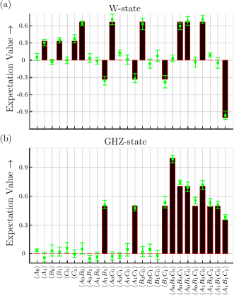
Figure 2: Bar plots for the observable moments of the moment matrix $\Gamma$ for (a) W and (b) GHZ states. Bars represent theoretically expected values while green squares are the experimentally observed values.

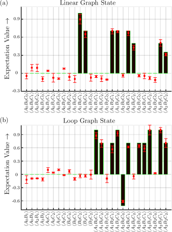
Figure 3: Bar plots for the observable moments of the moment matrix $\Gamma$ for (a) Linear and (b) Loop graph states. Bars represent theoretically expected values while green squares are the experimentally observed values.

As an example, the moment/correlator $\Gamma_{4,12}$ in the case of W state, is an observable $\sigma_{1x}\sigma_{2x}\sigma_{3z}$ while the moment/correlator $\Gamma_{1,18}$ is $-i\sigma_{2y}$ which is not an observable and enters the moment matrix as an SDP variable. Similarly one can compute the parameters for (3,3,2) scenario. The next task was to find the expectation values of the correlators in the state under investigation. In NMR experiments the observed signal is proportional to the $z$-magnetization of the ensemble which indeed is proportional to the expectation value of the Pauli $z$-spin angular momentum operator in the given state. Hence the direct observable in a typical NMR experiment is the Pauli $z$-operator expectation values of the nuclear spins. We have previously developed schemes to find the expectation values of any desired Pauli operators in the given state (Singh et al., 2016, 2018a, 2018b). This was achieved by mapping the state $\rho\rightarrow\rho_{l}=U_{l}.\rho.U_{l}^{\dagger}$ followed by $z$-magnetization measurement. The explicit forms of the unitary operators $U_{l}$, as well as quantum circuits and NMR pulse sequences, for two and three-qubit Pauli spin operators are given in Refs. (Singh et al., 2016) and (Singh et al., 2018a), respectively. As an example, for the measurement of the moment $\sigma_{1x}\sigma_{2x}\sigma_{3x}$, the form of $U_{l}=CNOT_{23}.\overline{Y}_{3}.CNOT_{12}.\overline{Y}_{2}.\overline{Y}_{1}$ can be utilize to construct the quantum circuit (Singh et al., 2018a). Similarly any desired moment can be measured precisely utilizing these techniques.

As stated earlier, the information regarding local/non-local nature of the observed correlations gets encoded in the measured correlators $\{\langle A_{x}\rangle,\;\langle B_{y}\rangle,\;\langle C_{z}\rangle,\;\langle A_{x}B_{y}\rangle,$ $\langle A_{x}C_{z}\rangle,\;\langle B_{y}C_{z}\rangle,\;\langle A_{x}B_{y}C_{z}\rangle\}$. The formulated SDP in all the cases, i.e. W, GHZ and graph states, failed to find $\Gamma\geq 0$ at the second level of the modified NPA hierarchy. This confirmed that the observed correlations can not arise from the local measurements on a separable state and hence the states are genuinely entangled. A bar plot for the observable moments of the moment matrix $\Gamma$ for W-state and GHZ-state is depicted in Fig.2(a) and Fig.2(b), respectively. Fig.3(a) and Fig.3(b) shows the results for linear and loop graph states respectively. It is interesting to note from the bar plots of Fig(2) that the correlations of GHZ state are mostly encoded in the full three-body correlators while for the W state fewer body moments are also able to capture the information about genuine entanglement. Similarly, one can observe in Fig.3 the role of various moments in encoding the information about the correlations for the linear as well as loop graph states. It may be noted here that only experimentally non-vanishing moments are shown in Fig.3 for graph states while Fig.2 shows all the observed moments in case of W as well as GHZ states.

In all the cases, the SDP was also formulated directly from experimentally reconstructed density matrices using full quantum state tomography. This verified and further supported the results of the modified NPA protocol obtained via direct measurements of the correlators. We note here in passing that the experimental protocol demonstration was on pure states, but the scheme is also capable of detecting non-locality of states which are a convex sum of white noise and pure states, up to a certain degree of mixedness (Baccari et al., 2017).

IV Concluding remarks

Local measurement-based hierarchies can be used to detect the presence of non-local correlations in a composite quantum system. A modified NPA hierarchy was used to detect the non-local nature of the tripartite correlations in a system of three qubits, by performing local measurements evolved via a semi-definite program. A set comprising of products and/or linear superpositions of such products of local projectors was defined and an associated positive semi-definite moment matrix was set up. Non-local correlation detection protocols typically require the experimental measurement of some correlator, in order to generate the statistics to be tested. Once the moment matrix embedded with the empirical data is obtained, the semi-definite program optimizes to obtain a positive moment matrix, under some linear constraints on the entries of the moment matrix, to check if the observed correlations can arise from local measurements on a separable state. The protocol was tested experimentally on three-qubit W, GHZ and a few graph states utilizing NMR hardware. In all the cases, the resulting SDP turned out to be unfeasible at the second level of the modified hierarchy, implying successful detection of the non-local nature of the observed correlation. The results were also verified by direct full quantum state tomography and then directly computing the correlators to formulate the SDP. Future directions of research include evaluating the performance of the protocol in higher dimensions as well as for more number of entangled parties, since the structure of the entanglement classes is more complex in a higher-dimensional Hilbert space.