Logical Differencing in Dyadic Network Formation Models with Nontransferable Utilities

Abstract

This paper considers a semiparametric model of dyadic network formation under nontransferable utilities (NTU). Such dyadic links arise frequently in real-world social interactions that require bilateral consent but by their nature induce additive non-separability. In our model we show how unobserved individual heterogeneity in the network formation model can be canceled out without requiring additive separability. The approach uses a new method we call logical differencing. The key idea is to construct an observable event involving the intersection of two mutually exclusive restrictions on the fixed effects, while these restrictions are as necessary conditions of weak multivariate monotonicity. Based on this identification strategy we provide consistent estimators of the network formation model under NTU. Finite-sample performance of our method is analyzed in a simulation study, and an empirical illustration using the risk-sharing network data from Nyakatoke demonstrates that our proposed method is able to obtain economically intuitive estimates.

Keywords: dyadic network formation, semiparametric estimation, nontransferable utilities, additive nonseparability

1 Introduction

This paper considers a semiparametric model of dyadic network formation under nontransferable utilities (NTU), which arise naturally in the modeling of real-world social interactions that require bilateral consent. For instance, friendship is usually formed only when both individuals in question are willing to accept each other as a friend, or in other words, when both individuals derive sufficiently high utilities from establishing the friendship. It is often plausible that the two individuals may derive very different utilities from the friendship for a variety of reasons: for example, one of them may simply be more introvert than the other and derive lower utilities from the friendship. In addition, there may not be a feasible way to perfectly transfer utilities between the two individuals. Monetary payments may not be customary in many social contexts, and even in the presence of monetary or in-kind transfers, utilities may not be perfectly transferable through these feasible forms of transfers, say, when individuals have different marginal utilities with respect to these transfers. Given the considerable academic and policy interest in understanding the underlying drivers of network formation, it is not only theoretically interesting but also empirically relevant to incorporate NTU in the modeling of network formation.

This paper contributes to the line of econometric literature on network formation by introducing and incorporating nontransferable utilities into dyadic network formation models. Previous work in this line of literature focuses primarily on case of transferable utilities, as represented in Graham (2017), which considers a parametric model with homophily effects and individual unobserved heterogeneity of the following form:

$$D_{ij}=\mathbf{\mathbbm{1}}\left\{w\left(X_{i},X_{j}\right)^{{}^{\prime}}\beta_{0}+A_{i}+A_{j}\geq\epsilon_{ij}\right\}$$ (1)

where $D_{ij}$ is an observable binary variable that denotes the presence or absence of a link between individual $i$ and $j$, $w\left(X_{i},X_{j}\right)$ represents a (symmetric) vector of pairwise observable characteristics specific to $ij$ generated by a known function $w$ of the individual observable characteristics $X_{i}$ and $X_{j}$ of $i$ and $j$, while $A_{i}$ and $A_{j}$ stand for unobserved individual-specific degree heterogeneity and $\epsilon_{ij}$ is some idiosyncratic utility shock. Model (1) essentially says that, if the (stochastic) joint surplus generated by a bilateral link $s_{ij}:=w\left(X_{i},X_{j}\right)^{{}^{\prime}}\beta_{0}+A_{i}+A_{j}-\epsilon_{ij}$ exceeds the threshold zero, then the link between $i$ and $j$ is formed. The model implicitly assumes that the link surplus can be freely distributed among the two individuals $i$ and $j$, and that bargaining efficiency is always achieved, so that the undirected link is formed if and only if the link surplus is positive. Given this specification, Graham (2017) provides consistent and asymptotically normal maximum-likelihood estimates for the homophily effect parameter $\beta_{0}$, assuming that the exogenous idiosyncratic pairwise shocks $\epsilon_{ij}$ are independently and identically distributed with a logistic distribution. Recently, Candelaria (2016) and Toth (2017) provide semiparametric generalizations of Graham (2017), while Gao (2020) established nonparametric identification of a class of index models that further generalize (1).

This paper, however, generalizes Graham (2017) along a different direction, and seeks to incorporate the natural micro-theoretical feature of NTU into this class of network formation models. To illustrate, consider the following simple adaption of model (1) with two threshold-crossing conditions:

$$D_{ij}=\mathbf{\mathbbm{1}}\left\{w\left(X_{i},X_{j}\right)^{{}^{\prime}}\beta_{0}+A_{i}\geq\epsilon_{ij}\right\}\cdot\mathbf{\mathbbm{1}}\left\{w\left(X_{i},X_{j}\right)^{{}^{\prime}}\beta_{0}+A_{j}\geq\epsilon_{ji}\right\},$$ (2)

where the unobserved individual heterogeneity $A_{i}$ and $A_{j}$ separately enter into two different threshold-crossing conditions. This formulation could be relevant to scenarios where $A_{i}$ represents individual $i$’s own intrinsic valuation of a generic friend: for a relatively shy or introvert person $i$, a lower $A_{i}$ implies that $i$ is less willing to establish a friendship link, regardless of how sociable the counterparty is. For simplicity, suppose for now that $w\left(X_{i},X_{j}\right)\equiv{\bf 0}$, $\epsilon_{ij}\sim_{iid}F$, $\epsilon_{ji}\sim_{iid}F$ and $\epsilon_{ij}\perp\epsilon_{ji}$. Focusing completely on the effects of $A_{i}$ and $A_{j}$, it is clear that the TU model (1) implies that only the sum of “sociability”, $A_{i}+A_{j}$, matters: the linking probability among pairs with $A_{i}=A_{j}=1$ (two moderately social persons) should be exactly the same as the linking probability among pairs with $A_{i}=2$ and $A_{j}=0$ (one very social person and one very shy person), which might not be reasonable or realistic in social scenarios. In comparison, the linking probability among pairs with $A_{i}=2$ and $A_{j}=0$ is lower than the linking probability among pairs with $A_{i}=A_{j}=1$ under the NTU model (2) with i.i.d. $\epsilon_{ij}$ and $\epsilon_{ji}$ that follow any log-concave distribution:

$$\mathbb{E}\left[\left.D_{ij}\right|w\left(X_{i},X_{j}\right)\equiv{\bf 0},A_{i}=2,A_{j}=0\right]$$

$$=\ F\left(0\right)F\left(2\right)$$

$$<\ F\left(1\right)F\left(1\right)$$

$$=\ \mathbb{E}\left[\left.D_{ij}\right|w\left(X_{i},X_{j}\right)\equiv{\bf 0},A_{i}=A_{j}=1\right]$$

This is intuitive given the observation that, under bilateral consent, the party with relatively lower utility is the pivotal one in link formation. Moreover, even though we maintain strict monotonicity in the unobservable characteristics $A_{i}$ and $A_{j}$, the NTU setting can still effectively incorporate homophily effects on unobserved heterogeneity: given that $w\left(X_{i},X_{j}\right)\equiv{\bf 0}$ and $A_{i}+A_{j}=2$, the linking probability is effectively decreasing in $\left|A_{i}-A_{j}\right|$ under log-concave $F$. Hence, by explicitly modeling NTU in dyadic network formation, we can accommodate more flexible or realistic patterns of conditional linking probabilities and homophily effects that are not present under the TU setting.

However, the NTU setting immediately induces a key technical complication: as can be seen explicitly in model (2), the observable indexes, $w\left(X_{i},X_{j}\right)^{{}^{\prime}}\beta_{0}$ and $w\left(X_{j},X_{i}\right)^{{}^{\prime}}\beta_{0}$, and the unobserved heterogeneity terms ($A_{i}$ and $A_{j}$) are no longer additively separable from each other. In particular, notice that, even though the utility specification for each individual inside each of the two threshold-crossing conditions in model (2) remains completely linear and additive, the multiplication of the two (nonlinear) indicator functions directly destroys both linearity and additive separability, rendering inapplicable most previously developed econometric techniques that arithmetically “difference out” the “two-way fixed effects” $A_{i}$ and $A_{j}$ based on additive separability.

Given this technical challenge, this paper proposes a new identification strategy termed logical differencing, which helps cancel out the unobserved heterogeneity terms, $A_{i}$ and $A_{j}$, without requiring additive separability but leveraging the logical implications of multivariate monotonicity in model (2). The key idea is to construct an observable event involving the intersection of two mutually exclusive restrictions on the fixed effects $A_{i}$ and $A_{j}$, which logically imply an event that can be represented without $A_{i}$ or $A_{j}$. Specifically, in the context of the illustrative model (2) above, we start by considering the event where a given individual $\overline{i}$ is more popular than another individual $\overline{j}$ among a group of individuals $k$ with observable characteristics $X_{k}=\overline{x}$ while $\overline{i}$ is simultaneously less popular than another individual $\overline{j}$ among a group of individuals with a certain realization of observable characteristics $\underline{x}$. This is the same as the conditioning event in Toth (2017) and analogous to the tetrad comparisons made in Candelaria (2016). However, instead of using arithmetic differencing to cancel out the unobserved heterogeneity $A_{\overline{i}}$ and $A_{\overline{j}}$ as in Candelaria (2016) and Toth (2017), we make the following logical deductions based on the monotonicity of the conditional popularity of $\overline{i}$ in $w\left(X_{\overline{i}},\overline{x}\right)^{{}^{\prime}}\beta_{0}$ and $A_{\overline{i}}$. First, the event that $\overline{i}$ is more popular than another individual $\overline{j}$ among the group of individuals with $X_{k}=\overline{x}$ implies that either $w\left(X_{\overline{i}},\overline{x}\right)^{{}^{\prime}}\beta_{0}>w\left(X_{\overline{j}},\overline{x}\right)^{{}^{\prime}}\beta_{0}$ or $A_{\overline{i}}>A_{\overline{j}}$, while the event that $\overline{i}$ is less popular than another individual $\overline{j}$ among a different group of individuals with $X_{l}=\underline{x}$ implies that either $w\left(X_{\overline{i}},\underline{x}\right)^{{}^{\prime}}\beta_{0}<w\left(X_{\overline{j}},\underline{x}\right)^{{}^{\prime}}\beta_{0}$ or $A_{\overline{i}}<A_{\overline{j}}$. Second, when both events occur simultaneously, we can logically deduce that either $w\left(X_{\overline{i}},\overline{x}\right)^{{}^{\prime}}\beta_{0}>w\left(X_{\overline{j}},\overline{x}\right)^{{}^{\prime}}\beta_{0}$ or $w\left(X_{\overline{i}},\underline{x}\right)^{{}^{\prime}}\beta_{0}<w\left(X_{\overline{j}},\underline{x}\right)^{{}^{\prime}}\beta_{0}$ must have occurred, because $A_{\overline{i}}>A_{\overline{j}}$ and $A_{\overline{i}}<A_{\overline{j}}$ cannot simultaneously occur. Intuitively, the “switch” in the relative popularity of $\overline{i}$ and $\overline{j}$ among the two groups of individuals with characteristics $\overline{x}$ and $\underline{x}$ cannot be driven by individual unobserved heterogeneity $A_{\overline{i}}$ and $A_{\overline{j}}$, and hence when we indeed observe such a “switch”, we obtain a restriction on the parametric indices $w\left(X_{\overline{i}},\overline{x}\right)^{{}^{\prime}}\beta_{0}$, $w\left(X_{\overline{i}},\overline{x}\right)^{{}^{\prime}}\beta_{0}$, $w\left(X_{\overline{i}},\underline{x}\right)^{{}^{\prime}}\beta_{0}$, and $w\left(X_{\overline{j}},\underline{x}\right)^{{}^{\prime}}\beta_{0}$, which helps identify $\beta_{0}$.

Based on this identification strategy we provide sufficient conditions for point identification of the parameter $\beta_{0}$ up to scale normalization as well as a consistent estimator for $\beta_{0}$. Our estimator has a two-step structure, with the first step being a standard nonparametric estimator of conditional linking probabilities, which we use to assert the occurrence of the conditioning event, while in the second step we use the identifying restriction on $\beta_{0}$ when the conditioning event occurs. The computation of the estimator essentially follows the same method proposed in Gao and Li (2021), with some adaptions to the network data setting. We plot the identified sets under various restrictions on the support of the observable characteristics $X_{i}$, analyze the finite-sample performance in a simulation study, and present an empirical illustration of our method using data from Nyakatoke on risk-sharing network collected by Joachim De Weerdt.

This paper belongs to the line of literature that studies dyadic network formation in a single large network setting, including Blitzstein and Diaconis (2011), Chatterjee, Diaconis, and Sly (2011), Yan and Xu (2013), Yan, Leng, and Zhu (2016), Graham (2017), Charbonneau (2017), Dzemski (2017), Jochmans (2017), Yan, Jiang, Fienberg, and Leng (2018), Candelaria (2016), Toth (2017) and Gao (2020). Shi and Chen (2016) explicitly incorporates NTU into dyadic network formation models, but Shi and Chen (2016) considers a fully parametric model and establishes the consistency and asymptotic normality of the maximum likelihood estimators. See also the recent surveys by de Paula (2020a) and Graham (2020).

This paper is also related to a line of research that utilizes dyadic link formation models in order to study structural social interaction models: for instance, Arduini et al. (2015), Auerbach (2019), Goldsmith-Pinkham and Imbens (2013), Hsieh and Lee (2016) and Johnsson and Moon (2021). In these papers, the social interaction models are the main focus of identification and estimation, while the link formation models are used mainly as a tool (a control function) to deal with network endogeneity or unobserved heterogeneity problems in the social interaction model. Even though some of the network formation models considered in this line of literature is consistent with the NTU setting, this line of literature is usually not primarily concerned with the full identification and estimation of the network formation model itself.

It should be pointed out that in this paper we do not consider link interdependence in network formation, which is studied by the line of econometric literature on strategic network formation models. This line of literature primarily uses pairwise stability (Jackson and Wolinsky, 1996) as the solution concept for network formation, and also often builds NTU into the econometric specification. See, for example, De Paula, Richards-Shubik, and Tamer (2018), Graham (2016), Leung (2015), Menzel (2017), Boucher and Mourifié (2017), Mele (2017a), Mele (2017b) and Ridder and Sheng (2017). However, this type of models usually do not feature unobserved heterogeneity as in this paper. See, for example, de Paula (2020b) for a more detailed survey on this line of literature.

This paper is also closely related to to Gao and Li (2021), which similarly leverages multivariate monotonicity in a multi-index structure under a panel multinomial choice setting. It should be pointed out that, even though there is some structural similarity between network data and panel data, there are no direct ways in the network setting to make “intertemporal comparison” as in the panel setting, which holds the fixed effects unchanged across two observable periods of time. It is precisely this additional complication induced by the network setting that requires the technique of logical differencing proposed in this paper.

The rest of the paper is organized as follows. In Section 2, we describe the general specifications of our dyadic network formation model. Section 3 establishes identification of the parameter of interests in our model and provides a consistent tetrad estimator. We plot the identified sets under various restrictions on $X$ and report baseline simulation results in Section 4. We present an empirical illustration using the risk-sharing data of Nyakatoke in Section 5. Section 6 concludes. Proofs and additional simulation results are available in the Appendix.

2 A Nonseparable Dyadic Network Formation Model

We consider the following dyadic network formation model:

$$\mathbb{E}\left[\left.D_{ij}\right|X_{i},X_{j},A_{i},A_{j}\right]=\phi\left(w\left(X_{i},X_{j}\right)^{{}^{\prime}}\beta_{0},A_{i},A_{j}\right)$$ (3)

where:

• $i\in\left\{1,...,n\right\}$ denote a generic individual in a group of $n$ individuals.

• $X_{i}$ is a $\mathbb{R}^{d_{x}}$-valued vector of observable characteristics for individual $i$. This could include, for example, wealth, age, education and ethnicity of individual $i$.

• $D_{ij}$ denotes a binary observable variable that indicates the presence or absence of an undirected and unweighted link between two distinct individuals $i$ and $j$: $D_{ij}=D_{ji}$ for all pairs of individuals $ij$, with $D_{ij}=1$ indicating that $ij$ are linked while $D_{ij}=0$ indicating that $ij$ are not linked.

• $w:\mathbb{R}^{d_{x}}\times\mathbb{R}^{d_{x}}\to\mathbb{R}^{d}$ is a known function that is symmetric with respect to its two vector arguments. We will write $W_{ij}:=w\left(X_{i},X_{j}\right)$ for notational simplicity.

• $\beta_{0}\in\mathbb{R}^{d}$ is an unknown finite-dimensional parameter of interest. Assume $\beta_{0}\neq{\bf 0}$ so that we may normalize $\left\|\beta_{0}\right\|=1$, i.e., $\beta_{0}\in\mathbb{\mathbb{S}}^{d-1}$.

• $A_{i}$ is an unobserved scalar-valued variable that represents unobserved individual heterogeneity.

• $\phi:\mathbb{R}^{3}\to\mathbb{R}$ is an unknown measurable function that is symmetric with respect to its second and third arguments.

In addition, we impose the following two assumptions:

Assumption 1 (Monotonicity).

$\phi$ is weakly increasing in each of its arguments.

Assumption 1 is the key assumption on which our identification analysis is based. It requires that the conditional linking probability between individuals with characteristics $\left(X_{i},A_{i}\right)$ and $\left(X_{j},A_{j}\right)$ be monotone in a parametric index $\delta_{ij}:=W_{ij}^{{}^{\prime}}\beta_{0}$ as well as the unobserved individual heterogeneity terms $A_{i}$ and $A_{j}$. It should be noted that, given monotonicity, increasingness is without loss of generality as $\phi$, $\beta_{0}$ and $A_{i},A_{j}$ are all unknown or unobservable. In addition, Assumption 1 only requires that $\phi$ is monotonic in the index $W_{ij}^{{}^{\prime}}\beta_{0}$ as a whole, not individual coordinates of $W_{ij}$. Therefore, we may include nonlinear or non-monotone functions $w\left(\cdot,\cdot\right)$ on the observable characteristics as long as Assumption 1 is maintained.

Next, we impose a standard random sampling assumption:

Assumption 2 (Random Sampling).

$\left(X_{i},A_{i}\right)$ is i.i.d. across $i\in\left\{1,...,n\right\}$.

In particular, Assumption 2 allows arbitrary dependence structures between the observable characteristics $X_{i}$ and the unobservable characteristic $A_{i}$.

Model (3) along with the specifications and the two assumptions introduced above encompass a large class of dyadic network formation models in the literature. For example, the standard dyadic network formation model (1) studied by Graham (2017) can be written as

$$\mathbb{E}\left[\left.D_{ij}\right|X_{i},X_{j},A_{i},A_{j}\right]=F\left(W_{ij}^{{}^{\prime}}\beta_{0}+A_{i}+A_{j}\right)$$

where $F$ is the CDF of the standard logistic distribution. For the semiparametric version considered by Candelaria (2016), Toth (2017), and Gao (2020), we can simply take $F$ to be some unknown CDF. In either case, the monotonicity of the CDF $F$ and the additive structure of $W_{ij}^{{}^{\prime}}\beta_{0}+A_{i}+A_{j}$ immediately imply Assumption 1.

However, our current model specification and assumptions further incorporate a larger class of dyadic network formation models with potentially nontransferable utilities. Specifically, consider the joint requirement of two threshold-crossing conditions

$$D_{ij} =\mathbf{\mathbbm{1}}\left\{u\left(W_{ij}^{{}^{\prime}}\beta_{0},A_{i},A_{j},\epsilon_{ij}\right)\geq 0\right\}\cdot\mathbf{\mathbbm{1}}\left\{u\left(W_{ji}^{{}^{\prime}}\beta_{0},A_{j},A_{i},\epsilon_{ji}\right)\geq 0\right\},$$ (4)

where $u$ is an unknown function that is not necessarily symmetric with respect to its second and third arguments $\left(A_{i},A_{j}\right)$, and $\left(\epsilon_{ij},\epsilon_{ji}\right)$ are idiosyncratic pairwise shocks that are i.i.d. across each unordered $ij$ pair with some unknown distribution. In particular, notice that model (2) is a special case of (4). Suppose we further impose the following two lower-level assumptions 1a and 1b:

Assumption (1a).

$\left(\epsilon_{ij},\epsilon_{ji}\right)$ are independent of $\left(X_{i},A_{i},X_{j},A_{j}\right)$.

Assumption (1b).

$u$ is weakly increasing in its first three arguments.

Then, the conditional linking probability

$$\ \mathbb{E}\left[\left.D_{ij}\right|X_{i},X_{j},A_{i},A_{j}\right]$$

$$= \ \int\mathbf{\mathbbm{1}}\left\{u\left(W_{ij}^{{}^{\prime}}\beta_{0},A_{i},A_{j},\epsilon_{ij}\right)\geq 0\right\}\cdot\mathbf{\mathbbm{1}}\left\{u\left(W_{ji}^{{}^{\prime}}\beta_{0},A_{j},A_{i},\epsilon_{ji}\right)\geq 0\right\}d\mathbb{P}\left(\epsilon_{ij},\epsilon_{ji}\right)$$

$$=: \ \phi\left(W_{ij}^{{}^{\prime}}\beta_{0},A_{i},A_{j}\right)$$ (5)

can be represented by model (3) with Assumption 1 satisfied.

In particular, we do not require $\epsilon_{ij}\perp\epsilon_{ji}$. In fact, $\epsilon_{ij}\equiv\epsilon_{ji}$ is readily incorporated in our model. Under the maintained assumption that $w\left(X_{i},X_{j}\right)=w\left(X_{j},X_{i}\right)$, if $\epsilon_{ij}\equiv\epsilon_{ji}$ and $u$ is furthermore assumed to be symmetric with respect to its second and third arguments ($A_{i}$ and $A_{j}$), then our model specializes to the case of transferable utilities,

$$D_{ij}=\mathbf{\mathbbm{1}}\left\{u\left(W_{ij}^{{}^{\prime}}\beta_{0},A_{i},A_{j},\epsilon_{ij}\right)\geq 0\right\},$$

where effectively only one threshold crossing condition determines the establishment of a given network link. Therefore, our NTU model (3) includes the TU model as a special case.

Remark 1 (Symmetry of $w$).

To explain the key idea of our identification strategy in a notation-economical way, we will be focusing on the case of symmetric $w$ in most of the following sections. However, it should be pointed out that our method can also be applied to the case where $w$ is allowed to be asymmetric in (4), so that individual utilities based on observable characteristics can also be made asymmetric (nontransferable). In that case, model (4) needs to be modified as

$$\mathbb{E}\left[\left.D_{ij}\right|X_{i},X_{j},A_{i},A_{j}\right]=\phi\left(W_{ij}^{{}^{\prime}}\beta_{0},W_{ji}^{{}^{\prime}}\beta_{0},A_{i},A_{j}\right),$$ (6)

where $W_{ij}=w\left(X_{i},X_{j}\right)$ may be different from $W_{ji}=w\left(X_{j},X_{i}\right)$, but $\phi$ is symmetric with respect to its first two arguments $W_{ij}^{{}^{\prime}}\beta_{0},W_{ji}^{{}^{\prime}}\beta_{0}$ whenever $A_{i}=A_{j}$ Moreover, Assumption 1 should also be changed to be $\phi$ is monotone in all its four arguments. See Appendix C for a more detailed discussion on how our identification strategy can be adapted to accommodate asymmetric $w$ under appropriate conditions.

3 Identification and Estimation

3.1 Identification via Logical Differencing

In this section, we explain the key idea of our identification strategy. We construct a mutually exclusive event to cancel out the unobservable heterogeneity $A_{i}$ and $A_{j}$, which leads to an identifying restriction on $\beta_{0}$. We call this technique “logical differencing”.

For each fixed individual $\overline{i}$, and each possible $\overline{x}\in\mathbb{R}^{d_{x}}$, define

$$\rho_{\overline{i}}\left(\overline{x}\right):=\mathbb{E}\left[\left.D_{\overline{i}k}\right|X_{k}=\overline{x}\right]$$ (7)

as the linking probability of this specific individual $\overline{i}$ with a group of individuals, individually indexed by $k$, with the same observable characteristics $X_{k}=\overline{x}$ (but potentially different fixed effects $A_{k}$). Clearly, $\rho_{i}\left(\overline{x}\right)$ is directly identified from data in a single large network.

Suppose that individual $\overline{i}$ has observed characteristics $X_{\overline{i}}=x_{\overline{i}}$ and unobserved characteristics $A_{\overline{i}}=a_{\overline{i}}$. Then, by model (3) we have

$$\rho_{\overline{i}}\left(\overline{x}\right) =\mathbb{E}\left[\left.\mathbb{E}\left[\left.D_{\overline{i}k}\right|X_{k}=\overline{x},A_{k},X_{\overline{i}}=x_{\overline{i}},A_{\overline{i}}=a_{\overline{i}}\right]\right|X_{k}=\overline{x}\right]$$

$$=\mathbb{E}\left[\left.\phi\left(w\left(x_{\overline{i}},\overline{x}\right)^{{}^{\prime}}\beta_{0},a_{\overline{i}},A_{k}\right)\right|X_{k}=\overline{x}\right]$$

$$=:\psi_{\overline{x}}\left(w\left(x_{\overline{i}},\overline{x}\right)^{{}^{\prime}}\beta_{0},a_{\overline{i}}\right),$$ (8)

where the expectation in the second to last line is taken over $A_{k}$ conditioning on $X_{k}=\overline{x}$. As we allow $A_{k}$ and $X_{k}$ to be arbitrarily correlated, the $\psi_{\overline{x}}$ function defined in the last line of (8) is dependent on $\overline{x}$. In the same time, notice that $\psi_{\overline{x}}$ does not depend on the identity of $\overline{i}$ beyond the values of $w\left(x_{\overline{i}},\overline{x}\right)^{{}^{\prime}}\beta_{0}$ and $a_{\overline{i}}$. By Assumption 1, $\psi_{\overline{x}}\left(w\left(x_{\overline{i}},\overline{x}\right)^{{}^{\prime}}\beta_{0},a_{\overline{i}}\right)$ must be bivariate weakly increasing in the index $w\left(x_{\overline{i}},\overline{x}\right)^{{}^{\prime}}\beta_{0}$ and the unobserved heterogeneity scalar $a_{\overline{i}}$. We now show how to use the bivariate monotonicity to obtain identifying restrictions on $\beta_{0}$.

Fixing two distinct individuals $\overline{i}$ and $\overline{j}$ in the population, we first consider the event that individual $\overline{i}$ is strictly more popular than individual $\overline{j}$ among the group of individuals with observed characteristics $X_{k}=\overline{x}$:

$$\rho_{\overline{i}}\left(\overline{x}\right)>\rho_{\overline{j}}\left(\overline{x}\right),$$ (9)

which is an event directly identifiable from observable data given (7). Even though event (9) is the same conditioning event as considered in Toth (2017) and analogous to the tetrad comparisons made in Candelaria (2016), we now exploit the following logical deduction based on the bivariate monotonicity of the conditional popularity of $\overline{i}$ in $w\left(X_{\overline{i}},\overline{x}\right)^{{}^{\prime}}\beta_{0}$ and $A_{\overline{i}}$ without the assumption of additivity between them. Specifically, writing $\left(x_{\overline{i}},a_{\overline{i}}\right)$ and $\left(x_{\overline{j}},a_{\overline{j}}\right)$ as the observable and unobservable characteristics of individuals $\overline{i}$ and $\overline{j}$, by (8) we have

$$\rho_{\overline{i}}\left(\overline{x}\right)>\rho_{\overline{j}}\left(\overline{x}\right).$$

$$\Leftrightarrow\quad \psi_{\overline{x}}\left(w\left(x_{\overline{i}},\overline{x}\right)^{{}^{\prime}}\beta_{0},a_{\overline{i}}\right)>\psi_{\overline{x}}\left(w\left(x_{\overline{j}},\overline{x}\right)^{{}^{\prime}}\beta_{0},a_{\overline{j}}\right)$$

$$\Rightarrow\quad \left\{w\left(x_{\overline{i}},\overline{x}\right)^{{}^{\prime}}\beta_{0}>w\left(x_{\overline{j}},\overline{x}\right)^{{}^{\prime}}\beta_{0}\right\}\text{ OR }\left\{a_{\overline{i}}>a_{\overline{j}}\right\},$$ (10)

Note that the last line of equation (10) is a natural necessary (but not sufficient) condition for $\rho_{\overline{i}}\left(\overline{x}\right)>\rho_{\overline{j}}\left(\overline{x}\right)$ under bivariate monotonicity.

Now, consider the event that individual $\overline{i}$ is strictly less popular than individual $\overline{j}$ among the group of individuals with observed characteristics $X_{k}=\underline{x}$, i.e.,

$$\rho_{\overline{i}}\left(\underline{x}\right)<\rho_{\overline{j}}\left(\underline{x}\right).$$ (11)

Then, by a similar argument to (10), we deduce

$$\rho_{\overline{i}}\left(\underline{x}\right)<\rho_{\overline{j}}\left(\underline{x}\right)\quad\Rightarrow\quad\left\{w\left(x_{\overline{i}},\underline{x}\right)^{{}^{\prime}}\beta_{0}<w\left(x_{\overline{j}},\underline{x}\right)^{{}^{\prime}}\beta_{0}\right\}\text{ OR }\left\{a_{\overline{i}}<a_{\overline{j}}\right\}.$$ (12)

Notice that the event $\left\{a_{\overline{i}}<a_{\overline{j}}\right\}$ in (12) is mutually exclusive with the event $\left\{a_{\overline{i}}>a_{\overline{j}}\right\}$ that shows up in (10).

Next, consider the event that the two events (9) and (11) described above simultaneously happen. Then, by (10), (12) and basic logical operations, we have

$$\text{$\phantom{\text{ OR }}$ }\left\{\rho_{\overline{i}}\left(\overline{x}\right)>\rho_{\overline{j}}\left(\overline{x}\right)\right\}\text{ AND }\left\{\rho_{\overline{i}}\left(\underline{x}\right)<\rho_{\overline{j}}\left(\underline{x}\right)\right\}$$

$$\Rightarrow\quad \text{$\phantom{\text{ OR }}$ }\left(\left\{w\left(x_{\overline{i}},\overline{x}\right)^{{}^{\prime}}\beta_{0}>w\left(x_{\overline{j}},\overline{x}\right)^{{}^{\prime}}\beta_{0}\right\}\text{ OR }\left\{a_{\overline{i}}>a_{\overline{j}}\right\}\right)$$

AND  $$\left(\left\{w\left(x_{\overline{i}},\underline{x}\right)^{{}^{\prime}}\beta_{0}<w\left(x_{\overline{j}},\underline{x}\right)^{{}^{\prime}}\beta_{0}\right\}\text{ OR }\left\{a_{\overline{i}}<a_{\overline{j}}\right\}\right)$$

$$\Leftrightarrow\quad \phantom{\text{ OR }}\left(\left\{w\left(x_{\overline{i}},\overline{x}\right)^{{}^{\prime}}\beta_{0}>w\left(x_{\overline{j}},\overline{x}\right)^{{}^{\prime}}\beta_{0}\right\}\ \text{AND}\ \left\{w\left(x_{\overline{i}},\underline{x}\right)^{{}^{\prime}}\beta_{0}<w\left(x_{\overline{j}},\underline{x}\right)^{{}^{\prime}}\beta_{0}\right\}\right)$$

$$\text{ OR }\left(\left\{w\left(x_{\overline{i}},\overline{x}\right)^{{}^{\prime}}\beta_{0}>w\left(x_{\overline{j}},\overline{x}\right)^{{}^{\prime}}\beta_{0}\right\}\ \text{AND}\ \left\{a_{\overline{i}}<a_{\overline{j}}\right\}\right)$$

$$\text{ OR }\left(\left\{a_{\overline{i}}>a_{\overline{j}}\right\}\ \text{AND}\ \left\{w\left(x_{\overline{i}},\underline{x}\right)^{{}^{\prime}}\beta_{0}<w\left(x_{\overline{j}},\underline{x}\right)^{{}^{\prime}}\beta_{0}\right\}\right)$$

$$\text{ OR }\left(\left\{a_{\overline{i}}>a_{\overline{j}}\right\}\ \text{AND}\ \left\{a_{\overline{i}}<a_{\overline{j}}\right\}\right)$$

$$\Rightarrow\quad \phantom{\text{ OR }}\left(\left\{w\left(x_{\overline{i}},\overline{x}\right)^{{}^{\prime}}\beta_{0}>w\left(x_{\overline{j}},\overline{x}\right)^{{}^{\prime}}\beta_{0}\right\}\ \text{AND}\ \left\{w\left(x_{\overline{i}},\underline{x}\right)^{{}^{\prime}}\beta_{0}<w\left(x_{\overline{j}},\underline{x}\right)^{{}^{\prime}}\beta_{0}\right\}\right)$$

$$\text{ OR }\left\{w\left(x_{\overline{i}},\overline{x}\right)^{{}^{\prime}}\beta_{0}>w\left(x_{\overline{j}},\overline{x}\right)^{{}^{\prime}}\beta_{0}\right\}$$

$$\text{ OR }\left\{w\left(x_{\overline{i}},\underline{x}\right)^{{}^{\prime}}\beta_{0}<w\left(x_{\overline{j}},\underline{x}\right)^{{}^{\prime}}\beta_{0}\right\}$$

$$\Leftrightarrow\quad \left\{\left(w\left(x_{\overline{i}},\overline{x}\right)-w\left(x_{\overline{j}},\overline{x}\right)\right)^{{}^{\prime}}\beta_{0}>0\right\}\ \text{OR}\ \left\{\left(w\left(x_{\overline{i}},\underline{x}\right)-w\left(x_{\overline{j}},\underline{x}\right)\right)^{{}^{\prime}}\beta_{0}<0\right\},$$ (13)

The derivations above exploit two simple logical properties: first,

$$\left\{a_{\overline{i}}>a_{\overline{j}}\right\}\ \text{AND}\ \left\{a_{\overline{i}}<a_{\overline{j}}\right\}\quad=\quad\text{FALSE},$$

and second,

$$\left\{w\left(x_{\overline{i}},\overline{x}\right)^{{}^{\prime}}\beta_{0}>w\left(x_{\overline{j}},\overline{x}\right)^{{}^{\prime}}\beta_{0}\right\}\ \text{AND}\ \left\{a_{\overline{i}}<a_{\overline{j}}\right\}\quad\Rightarrow\quad\left\{w\left(x_{\overline{i}},\overline{x}\right)^{{}^{\prime}}\beta_{0}>w\left(x_{\overline{j}},\overline{x}\right)^{{}^{\prime}}\beta_{0}\right\},$$

which uses only necessary but not sufficient condition, so that we can obtain an identifying restriction (13) on $\beta_{0}$ that does not involve $a_{\overline{i}}$ nor $a_{\overline{j}}$. These two forms of logical operations together enable us to “difference out” (or “cancel out”) the unobserved heterogeneity terms $a_{\overline{i}}$ and $a_{\overline{j}}$.

In contrast with various forms of “arithmetic differencing” techniques proposed in the econometric literature (including Candelaria, 2016 and Toth, 2017 specific to the dyadic network formation literature), our proposed technique does not rely on additive separability between the parametric index $w\left(x_{\overline{i}},\overline{x}\right)^{{}^{\prime}}\beta_{0}$ and the unobserved heterogeneity term $a_{\overline{i}}$. Instead, our identification strategy is based on multivariate monotonicity and utilizes logical operations rather than standard arithmetic differencing to cancel out the unobserved heterogeneity terms. Hence, we term our method “logical differencing”.

The identifying arguments above are derived for a fixed pair of individuals $\overline{i}$ and $\overline{j}$, but clearly the arguments can be applied for any pair of individuals $\left(i,j\right)$ with observable characteristics $x_{i}$ and $x_{j}$. Writing

$$\tau_{ij}\left(\overline{x},\underline{x}\right) :=\mathbf{\mathbbm{1}}\left\{\rho_{i}\left(\overline{x}\right)>\rho_{j}\left(\overline{x}\right)\right\}\cdot\mathbf{\mathbbm{1}}\left\{\rho_{i}\left(\underline{x}\right)<\rho_{j}\left(\underline{x}\right)\right\}\text{ }\text{and}$$

$$\lambda\left(\overline{x},\underline{x};x_{i},x_{j};\beta\right) :=\mathbf{\mathbbm{1}}\left\{\left(w\left(x_{i},\overline{x}\right)-w\left(x_{j},\overline{x}\right)\right)^{{}^{\prime}}\beta_{0}\leq 0\right\}\cdot\mathbf{\mathbbm{1}}\left\{\left(w\left(x_{i},\underline{x}\right)-w\left(x_{j},\underline{x}\right)\right)^{{}^{\prime}}\beta_{0}\geq 0\right\}$$

for each $\beta\in\mathbb{\mathbb{S}}^{d-1}$, we summarize the identifying arguments above by the following lemma.

Lemma 1 (Identifying Restriction).

Under model (3) and Assumptions 1 and 2, we have

$$\tau_{ij}\left(\overline{x},\underline{x}\right)=1\quad\Rightarrow\quad\lambda\left(\overline{x},\underline{x};x_{i},x_{j};\beta_{0}\right)=0.$$ (14)

A simple (but clearly not unique) way to build a criterion function based on Lemma 1 is to define

$$Q\left(\beta\right):=\mathbb{E}_{ij,kl}\left[\tau_{ij}\left(X_{k},X_{l}\right)\lambda\left(X_{k},X_{l};X_{i},X_{j};\beta\right)\right],$$ (15)

where the expectation is $\mathbb{E}_{ij,kl}$ taken over random samples of ordered tetrads $\left(i,j,k,l\right)$ from the population, and $\left(X_{i},X_{j},X_{k},X_{l}\right)$ denote the random variables corresponding to the observable characteristics of $\left(i,j,k,l\right)$. According to Lemma 1, $Q\left(\beta_{0}\right)=0$, which is always smaller than or equal to $Q\left(\beta\right)\geq 0=Q\left(\beta_{0}\right)$ for any $\beta\neq\beta_{0}$ because $\tau_{ij}\geq 0$ and $\lambda\geq 0$ by construction.

Observing that the scale of $\beta_{0}$ is never identified, we write

$$B_{0}:=\left\{\beta\in\mathbb{\mathbb{S}}^{d-1}:Q\left(\beta\right)=0\right\}$$

to represent the normalized “identified set” relative to the criterion $Q$ defined in (15). Lemma 1 implies that $\beta_{0}\in B_{0}$, but in general there is no guarantee that $B_{0}$ is a singleton. The next subsection contains a set of sufficient conditions that guarantees $B_{0}=\left\{\beta_{0}\right\}$.

Remark 2.

We should point out that the identified set $B_{0}$ defined above based on logical differencing is not sharp in general, since the individual unobserved heterogeneity term $A_{i}$ is canceled out by logical differencing. In fact, one can show $A_{i}$ is also identified (up to proper normalization) under certain conditions, and knowledge about $A_{i}$ can help with the identification of $\beta_{0}$. In fact, when all realizations of $A_{i}$ are point identified, the point identification of $\beta_{0}$ can be established under much weaker conditions than those to be presented in Section 3.2. However, we trade sharpness for simplicity: this paper provides a method of identification (and estimation) without the need to deal with the incidental parameters $A_{i}$.

It is worth mentioning that for any one-sided sign preserving function $\gamma$ such that

$$\gamma\left(t\right)\ \begin{cases}\geq 0,&\text{for }t>0,\\ =0,&\text{for }t\leq 0.\end{cases}$$ (16)

we may define

$$\tau_{ij}^{\gamma}\left(\overline{x},\underline{x}\right) :=\gamma\left(\rho_{i}\left(\overline{x}\right)-\rho_{j}\left(\overline{x}\right)\right)\cdot\gamma\left(\rho_{j}\left(\underline{x}\right)-\rho_{i}\left(\underline{x}\right)\right),$$ (17)

$$Q^{\gamma}\left(\beta\right) :=\mathbb{E}_{ij,kl}\left[\tau_{ij}^{\gamma}\left(X_{k},X_{l}\right)\lambda\left(X_{k},X_{l};X_{i},X_{j};\beta\right)\right],$$ (18)

without changing the identification set at all, since

$$\tau_{ij}\left(\overline{x},\underline{x}\right)>0\quad\text{if and only if}\quad\tau_{ij}^{\gamma}\left(\overline{x},\underline{x}\right)>0.$$

In fact, $\tau^{\gamma}$ specializes to $\tau$ when we set $\gamma\left(t\right):=\mathbf{\mathbbm{1}}\left\{t>0\right\}$. Alternatively, we may set $\gamma$ to be “smoother”, say, $\gamma\left(t\right):=\left[t\right]_{+}$ the positive part function.

Such forms of “smoothing” in the population criterion will be irrelevant to all the identification results and its proofs in this paper, so for notational simplicity, we will suppress $\gamma$ and focus on the representative $\tau_{ij}$ and $Q$ in the next subsection about point identification. However, a smooth $\gamma$ will play a role when it comes to estimation and computation, and we will revisit $\gamma$ in Section 3.3.

3.2 Sufficient Conditions for Point Identification

We now present a set of sufficient conditions that guarantee point identification of $\beta_{0}$ on $\mathbb{\mathbb{S}}^{d-1}$.

Assumption 1^′ (Strict Monotonicity of $\phi$). $\phi$ defined in model (3) is weakly increasing in $A_{i}$ and $A_{j}$ while strictly increasing in the index $w\left(X_{i},X_{j}\right)^{{}^{\prime}}\beta_{0}$.

Assumption LABEL:as1prime strengthens Assumption 1 by requiring that $\phi$ be strictly increasing in the parametric index $w\left(X_{i},X_{j}\right)^{{}^{\prime}}\beta_{0}$. This is used to guarantee that differences in the parametric index can indeed lead to changes in conditional linking probabilities, so that the conditional event $\left\{\tau_{ij}\left(\overline{x},\underline{x}\right)=1\right\}$ in Lemma 1 may occur with strictly positive probability.

Assumption 3 (Continuity of $\phi$ and $w$).

$\phi$ and $w$ are continuous functions on their domains.

Assumption 4 (Sufficient Directional Variations).

There exist distinct points $\overline{x}$ and $\underline{x}$ in $Supp\left(X_{i}\right)$, such that the vector ${\bf 0}$ lies in the interior of $Supp\left(w\left(\overline{x},X_{i}\right)-w\left(\underline{x},X_{i}\right)\right)$.

We also provide a lower-level condition for Assumption 4 when $w$ is the coordinate-wise Euclidean distance function.

Assumption 4^′ Suppose that (i) $w_{h}\left(\overline{x},\underline{x}\right):=\left|\overline{x}_{h}-\underline{x}_{h}\right|$ for every coordinate $h$, and (ii) $Supp\left(X_{i}\right)$ has nonempty interior.

Essentially, since our criterion function is based on indicator functions of halfspaces in the form of $\left(w\left(\overline{x},\tilde{x}\right)-w\left(\underline{x},\tilde{x}\right)\right)^{{}^{\prime}}\beta\lesseqqgtr 0$, we will need the distribution of these indicators to take both values $0$ and $1$ with strictly positive probabilities under any $\beta$, so that every possible $\beta$ different from $\beta_{0}$ can be differentiated from $\beta_{0}$ by the criterion function (up to scale normalization). Hence, we need sufficient variations in the observable covariates.

Assumption 4, though apparently not very transparent on its own, is actually implied by Assumption LABEL:as3prime. We note that the assumption of nonempty interior is a familiar one, which is often imposed for point identification in the literature, say, on maximum score estimation. Assumption LABEL:as3prime allows the support of all observable covariates to be bounded, but on the other hand require all covariates to be continuously distributed.

In Appendix B, we present an alternative set of assumptions that allow for the presence of discrete covariates, but require the existence of a “special covariate” with large (conditional) continuous support and nonzero coefficient, a la Horowitz (1992). Since the identification result with special covariate needs to be presented under a different scale normalization, we defer the results to the appendix.

Assumption 5 (Conditional Support of $A_{i}$).

$A_{i}$ is conditionally distributed on the same support given $X_{i}=x$ for any realization $x\in Supp\left(X_{i}\right)$.

Assumption 5 together with Assumption 2 implies that for two randomly sampled individuals $i,j$, there is a strictly positive probability of $A_{i}$ and $A_{j}$ being sufficiently close to each other, conditional on any realizations of $X_{i}$ and $X_{j}$. Together with the continuity condition in Assumption 3, we can ensure that the parametric index based on observable covariates alone can determine whether $i$ or $j$ is relatively more popular among a certain group of individuals.

  

Next, we lay out the lemma that will be used in the proof of point identification of $\beta_{0}$.

Lemma 2 (Differentiating $\beta$ from $\beta_{0}$).

Under model (3), Assumptions LABEL:as1prime, 2–5, for each $\beta\in\text{$\mathbb{S}$}^{d-1}\backslash\left\{\beta_{0}\right\}$,

$$\tau_{ij}\left(X_{k},X_{l}\right) =1,$$ (19)

$$\lambda\left(X_{k},X_{l};X_{i},X_{j};\beta_{0}\right) =0,$$ (20)

$$\lambda\left(X_{k},X_{l};X_{i},X_{j};\beta\right) =1,$$ (21)

occur simultaneously with strictly positive probability, as we randomly sample individuals $i,j,k,l$.

For point identification of $\beta_{0}$, we need the population criterion (15) to differentiate each $\beta\in\text{$\mathbb{S}$}^{d-1}\backslash\left\{\beta_{0}\right\}$ from $\beta_{0}$. Lemma 2 ensures this by establishing that, the conditioning event (19) in Lemma 1 occurs with positive probability, and, when it occurs, we can obtain different values of $\lambda$ at $\beta$ from that at $\beta$ with positive probabilities. Compared with the set identification result discussed in Section 3.1, we need to strengthen Assumption 1 to strict monotonicity in the index $w\left(X_{i},X_{j}\right)^{{}^{\prime}}\beta_{0}$. Then, Assumptions 3 and 5 guarantee that, when the absolute difference between $A_{i}$ and $A_{j}$ get sufficiently small, differences in the parametric indexes can lead to differences in conditional linking probabilities, so that (19) will occur. Since $\beta_{0}$ and $\beta$ define different intersections of halfspaces for the vector $w\left(\overline{x},\tilde{x}\right)-w\left(\underline{x},\tilde{x}\right)$ through $\lambda$, Assumption 4 then guarantees that there will be on-support realizations of the observable covariates that help “detect” such differences.

We are now ready to present the point identification result.

Theorem 1 (Point Identification of $\beta_{0}$).

Under model (3) and Assumptions LABEL:as1prime, 2–5, $\beta_{0}$ is the unique minimizer of $Q\left(\beta\right)$ defined in (15) over the unit sphere $\text{$\mathbb{S}$}^{d-1}$. Furthermore, for any $\epsilon>0$, there exists $\delta>0$ such that

$$\inf_{\beta\in\text{$\mathbb{S}$}^{d-1}\backslash B_{\epsilon}\left(\beta_{0}\right)}Q\left(\beta\right)\geq Q\left(\beta_{0}\right)+\delta,$$

where $B_{\epsilon}\left(\beta_{0}\right):=\left\{\beta\in\mathbb{\mathbb{S}}^{d-1}:\|\beta-\beta_{0}\|\leq\epsilon\right\}$.

Theorem 1 follows from Lemma 2 based on the standard arguments in Newey and McFadden (1994).

Remark (Asymmetry of $w$, Continued).

In Appendix C, we show how the identification arguments and assumptions above can be adapted to accommodate asymmetry of $w$. In short, the technique of logical differencing applies without changes, but the identifying restriction we obtained becomes weaker. In particular, when $w$ is antisymmetric in the sense that $w\left(\overline{x},\underline{x}\right)+w\left(\underline{x},\overline{x}\right)\equiv 0$, the identifying restriction we obtained through logical differencing becomes trivial, and $B_{0}=\mathbb{\mathbb{S}}^{d-1}$. However, with asymmetric but not antisymmetric $w$, it is still feasible to strengthen Assumption 3 so as to obtain point identification. See more discussions in Appendix C.

3.3 Tetrad Estimator and Consistency

We now proceed to present a consistent estimator of $\beta_{0}$ in the framework of extremum estimation, which we construct using a two-step semiparametric estimation procedure. We clarify that we are considering the asymptotics under “a single large network” with the number of individuals $N\to\infty$. Moreover, we focus on the “dense network” asymptotics where the conditional linking probabilities are nondegenerate in the limit and can be consistently estimated.

The first step is the nonparametric estimation of

$$\rho_{i}\left(x\right):=\mathbb{E}\left[D_{ik}\big{|}i,X_{k}=x\right].$$

To implement this, we fix an individual $i$ in the sample, and regress $D_{ik}$, the indicator function for the link between $i$ and $k$, on the basis functions chosen by the researcher evaluated at observable characteristics $X_{k}$ for all $k\neq i$. To guarantee that a consistent nonparametric estimator of $\rho_{i}$ exists, we need to impose some regularity conditions on $\rho_{i}$. We state the following assumption as an illustrative set of such conditions, acknowledging that there may be many different versions that also work.

Assumption 6 (Regularity Conditions for $\rho_{i}$).

(i) $Supp\left(X_{i}\right)$ is bounded and convex with nonempty interior; (ii) for each fixed $i$, $\rho_{i}\in{\cal C}_{M}^{d_{x}+1}\left(Supp\left(X_{i}\right)\right)$, where ${\cal C}_{M}^{d_{x}+1}\left(Supp\left(X_{i}\right)\right)$ denotes the class of functions on $Supp\left(X_{i}\right)$ whose derivatives are uniformly bounded by $M$ up to order $d_{x}+1$.

Assumption 6 essentially requires that $\rho_{i}\left(x\right)$ is smooth enough in $x$. Given that

$$\rho_{i}\left(x\right)=\int\phi\left(w\left(\overline{x},x\right)^{{}^{\prime}}\beta_{0},a_{i},A_{k}\right)d\mathbb{P}\left(\left.A_{k}\right|X_{k}=x\right)$$

is an integral of $\phi$ (a strictly increasing function bounded between 0 and $1$) over the conditional distribution of $A_{k}$, Assumption 6 is easily satisfied, say, if both $\phi$ and the conditional density of $A_{k}$ given $X_{k}=x$ have uniformly bounded derivatives up to order $d+1$, when $w$ is taken to be the coordinate-wise Euclidean distance function.

Lemma 3.

Given Assumption 6, for each $i$, there exists an estimator $\hat{\rho}_{i}\in{\cal C}_{M}^{d_{x}+1}\left({\cal X}\right)$ that is $L_{2}\left(\mathbb{P}_{X}\right)$ consistent, i.e.,

$$\left\|\hat{\rho}_{i}-\rho_{i}\right\|_{L_{2}\left(\mathbb{P}_{X}\right)}:=\sqrt{\int\left(\hat{\rho}_{i}\left(x\right)-\rho_{i}\left(x\right)\right)^{2}d\mathbb{P}_{X_{k}}\left(x\right)}=o_{p}\left(1\right).$$

Lemma 3 follows from the large literature on many different types of consistent nonparametric estimators. See Bierens (1983) for results on kernel estimators and Chen (2007) on sieve estimators. In our simulation and application, we use a spline-based sieve estimator.

In the second step, we use $\hat{\rho}_{i}$ to build the following sample analog of the population criterion $Q^{\gamma}\left(\beta\right)$ in (15):

$$\widehat{Q}_{n}^{\gamma}\left(\beta\right):=\frac{\left(n-4\right)!}{n!}\sum_{i,j,k,l}\gamma\left(\hat{\rho}_{i}\left(X_{k}\right)-\hat{\rho}_{j}\left(X_{k}\right)\right)\gamma\left(\hat{\rho}_{j}\left(X_{l}\right)-\hat{\rho}_{i}\left(X_{l}\right)\right)\lambda\left(X_{k},X_{l};X_{i},X_{j};\beta\right).$$ (22)

The two-step tetrad estimator for $\beta_{0}$ is then defined as

$$\widehat{\beta}_{n}:=\arg\min_{\beta\in\text{$\mathbb{S}$}^{d-1}}\widehat{Q}_{n}^{\gamma}\left(\beta\right).$$ (23)

Since $\gamma$ can be arbitrarily chosen as long as it preserves strict positiveness as in Section 3.3, we now impose the following continuity assumption for $\gamma$.

Assumption 7 (Continuity of $\gamma$).

The one-sided sign-preserving function $\gamma$ is Lipschitz-continuous.

Assumption 7 can be achieved by setting, say, $\gamma\left(t\right):=\left[t\right]_{+}$ or $\gamma\left(t\right):=2\times\Phi\left(\left[t\right]_{+}\right)-1$, where $\left[t\right]_{+}$ is the positive part of $t$, and $\Phi$ is the CDF of the standard normal distribution. See Section 4 for details. The idea is that, when the difference $\rho_{i}\left(x\right)$ and $\rho_{j}\left(x\right)$ is small, the estimation of whether $\rho_{i}\left(x\right)>\rho_{j}\left(x\right)$ may be relatively imprecise, and therefore, we may wish to downweight such terms in the criterion function.

Computationally, to exploit the topological characteristics of the parameter space $\mathbb{\mathbb{S}}^{d-1}$, i.e. compactness and convexity, we develop a new bisection-style nested rectangle algorithm that recursively shrinks and refines an adaptive grid on the angle space. The key novelty of the algorithm is that instead of working with the edges of the Euclidean parameter space $\mathbb{R}^{d}$, we deterministically “cut” the angle space in each dimension of $\mathbb{\mathbb{S}}^{d-1}$ to search for the area that minimizes $\widehat{Q}_{n}^{\gamma}(\beta)$. Additional measures are taken to ensure the search algorithm is conservative. Simulation and empirical results show that our algorithm performs reasonably well with a relatively small sample size. Gao and Li (2021) provides more details regarding the implementation in a panel multinomial choice setting.

We now state the consistency result of the tetrad estimator $\widehat{\beta}_{n}$ under point identification.

Theorem 2.

Under model (3) and Assumptions LABEL:as1prime, 2–7, $\hat{\beta}_{n}$ is consistent for $\beta_{0}$, i.e.,

$$\widehat{\beta}_{n}\overset{p}{\longrightarrow}\beta_{0}.$$

Remark 3.

Our estimator shares some similarity with the maximum score estimator: the parameter $\beta$ enters into the sample criterion through indicators of halfspaces about $\beta$, which creates discreteness in the sample criterion. However, our estimator features an additional complication not found in maximum score estimation: we require the first-stage nonparametric estimators $\hat{\rho}_{i}$, and we need to plug the first-stage estimators into nonlinear functions that isolate the “positive side” only: $\gamma\left(\hat{\rho}_{i}\left(X_{k}\right)-\hat{\rho}_{j}\left(X_{k}\right)\right)\gamma\left(\hat{\rho}_{j}\left(X_{l}\right)-\hat{\rho}_{i}\left(X_{l}\right)\right)$ will be nonzero only when $\hat{\rho}_{i}\left(X_{k}\right)>\hat{\rho}_{j}\left(X_{k}\right)$ and $\hat{\rho}_{j}\left(X_{l}\right)>\hat{\rho}_{i}\left(X_{l}\right)$. In fact, it is precisely the “double-threshold” feature of our model that leads to the necessity of a semiparametric two-step estimation procedure, relative to the one-step procedure of the maximum score estimator under a “single-threshold” setting. Given that the asymptotic theory for the maximum score estimator is already nonstandard (with cubic-root rate of convergence and non-normal Chernoff-type asymptotic distribution as in Kim and Pollard, 1990), the addition of the first-stage nonparametric estimation further complicates the asymptotic theory to a highly nontrivial extent. The first-stage nonparametric estimation of $\rho_{i}$ may further slow the rate of convergence below $n^{-1/3}$; in the meanwhile, if we take $\gamma$ to be smooth (but necessarily nonlinear), the term $\gamma\left(\hat{\rho}_{i}\left(X_{k}\right)-\hat{\rho}_{j}\left(X_{k}\right)\right)\gamma\left(\hat{\rho}_{j}\left(X_{l}\right)-\hat{\rho}_{i}\left(X_{l}\right)\right)$ may also provide some effective smoothing on the discrete $\lambda_{ij}$ term, when $\rho_{i}\left(X_{k}\right)-\rho_{j}\left(X_{k}\right)$ or $\rho_{j}\left(X_{l}\right)-\rho_{i}\left(X_{l}\right)$ is closer to zero. It is not exactly clear which effect dominates, or whether the two effects can be balanced, in our current setting. Due to such technical difficulties, we defer the investigation of such types of “two-stage maximum score estimators” in a separate paper by Gao and Xu (2020), albeit in a simpler setting.

4 Simulation

In this section, we conduct a simulation study to analyze the finite-sample performance of our two-step tetrad estimator. To begin with, we calculate and plot the identified set $B_{0}$ via (15) for various support restrictions on $X$. The graph illustrates how the size of the identified set $B_{0}$ based on our population criterion (15) changes when the support of $X$ contains more and more discrete variables. Then, we specify the data generating process (DGP) of the Monte Carlo simulations. We show and discuss the performance of our two-step estimation method under the baseline setup with symmetric $w\left(\cdot,\cdot\right)$ function. In Appendix D, we vary the number of individuals $N$, the dimension of the pairwise observable characteristics $d$, and the degree of correlation between $X$ and $A$, as well as allow for asymmetric $w$ function to further examine the robustness of our method.

4.1 Identified Set $B_{0}$

In this section, we provide a graphical illustration of the identified set $B_{0}$ for various support restrictions on $X$. The analysis is based on the following network formation model:

$$D_{ij}=\mathbf{\mathbbm{1}}\left\{w\left(X_{i},X_{j}\right)^{{}^{\prime}}\beta_{0}+A_{i}>\epsilon_{ij}\right\}\cdot\mathbf{\mathbbm{1}}\left\{w\left(X_{j},X_{i}\right)^{{}^{\prime}}\beta_{0}+A_{j}>\epsilon_{ji}\right\},$$ (24)

where $w$ is taken to be the coordinate-wise absolute difference, i.e., $w_{h}\left(\overline{x},\underline{x}\right):=\left|\overline{x}_{h}-\underline{x}_{h}\right|$ for $h=1,...,d$. We set $d_{x}=d=3$ and $\beta_{0}=\left(1,1,1\right)/6^{{}^{\prime}}$. We incorporate correlation between $X$ and $A$ by drawing $A_{i}=\left(X_{i,1}+\xi_{i}\right)/4$, where $\xi_{i}$ is independently and uniformly distributed on $\left[-0.5,0.5\right]$ and independent of all other variables. $\epsilon_{ij}$ is the exogenous random shock independent of all other variables and uniformly distributed on $\left[0,1\right]$.

The purpose of the exercise is to show how the support restrictions on $X$ affect the size of the identified set $B_{0}$. To this end, we consider the following five support conditions on $X$: (1) all coordinates of $X$ are uniformly distributed on $[-0.5,0.5]$; (2) $X_{i,1}$ is binary with equal probability on $\left\{0,1\right\}$, while $X_{i,2}$ and $X_{i,3}$ are both uniformly distributed on $[-0.5,0.5]$; (3) $X_{i,1}$ is binary with equal probability on $\left\{0,1\right\}$, $X_{i,2}$ is discrete with equal probability on 11 points of $\left\{-0.5,-0.4,..,0,..,0.4,0.5\right\}$, and $X_{i,3}$ is uniformly distributed on $[-0.5,0.5]$; (4) all coordinates of $X$ are discrete with equal probability on 101 points of $\left\{-0.5,-0.49,-0.48..,0,..,0.49,0.5\right\}$; (5) all coordinates of $X$ are discrete with equal probability on 11 points of $\left\{-0.5,-0.4,..,0,..,0.4,0.5\right\}$.

$\beta_{0}$ is point identified in (1) since the support of $X$ has a nonempty interior, thus satisfying Assumption LABEL:as3prime. In (2)–(5), $\beta_{0}$ is not point identified due to discreteness and boundedness of the support of $X$. Below we compare the sizes of the identified sets when the $X$ vector contains none, one, two and all discrete variables corresponding to DGP (1)–(5).

To calculate the ID set, we utilize the analytical formula of $\rho_{i}$ so that the true $\rho_{i}$ is calculated without error . Then, we numerically approximate the population criterion by setting a large $N=1,000$ and $M=10,000$. We are able to work with a larger $N$ and $M$ than in the simulations in the next subsection because to get the identified set, we only calculate the maximizer of the population criterion once without the need to estimate $\rho_{i}\left(x\right)$. Still, one can improve the numerical results by increasing $N,M\rightarrow\infty$ and extracting more info from the data when additional computational power is available. Hence, all our results below are conservative: the true ID set must be a subset of the result shown in Figure 1.

For clarity of illustration, we plot the results in the angle space. In all cases, we maintain the correlation between $X$ and $A$. The results are summarized in Figure 1, where we plot the identified sets $B_{0}$ on the full parameter space of $\left[-\pi/2,\pi/2\right]\times\left[-\pi,\pi\right]$ and zoom it in for more details.

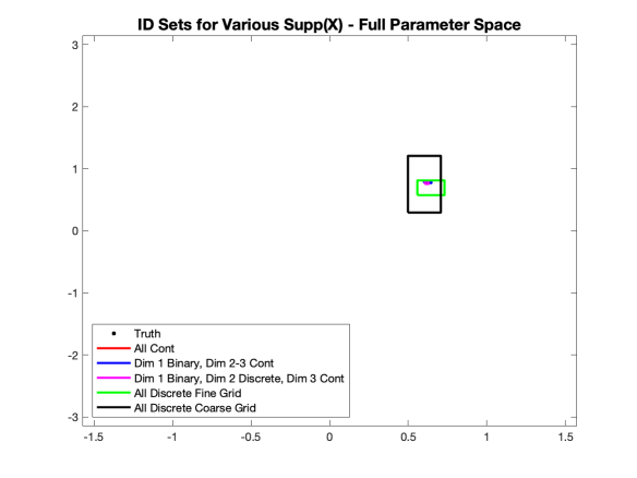
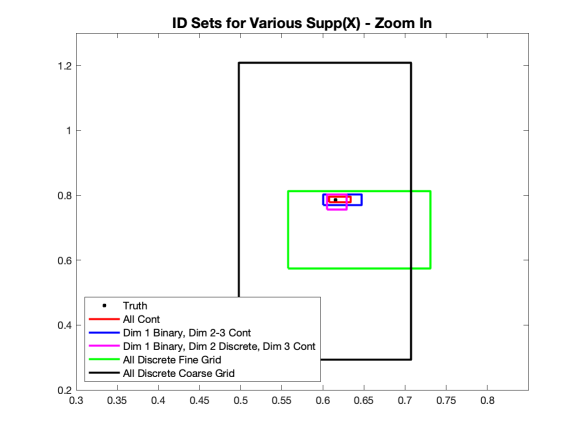
Figure 1: Identified Sets under Different Support Conditions for $X_{i}$

In Figure 1, the black dot represents the true $\beta_{0}$, which is guaranteed to belong to the identified set $B_{0}$. The red rectangle demonstrates the identified set when the supports of all coordinates of $X$ are continuous and bounded. The theory predicts point identification when the number of individuals $N$ and $\left(i,j\right)$ pairs $M$ go to infinity. Here the numerical result is indeed very close to point identification. The blue rectangle shows the identified set $B_{0}$ when the first dimension of $X$ is binary while all the other coordinates are continuous and bounded. The size of $B_{0}$ is larger than in case (1), which is expected due to the discreteness of $X_{i,1}$. The magenta rectangle corresponds to the case when $X_{i,1}$ is binary, $X_{i,2}$ is discrete, and $X_{i,3}$ is continuous and bounded. The size of $B_{0}$ is reasonably small, given that there are two discrete variables in $X$ and one of them is binary. The green and black rectangles illustrate $B_{0}$ when all coordinates of $X$ are discretely distributed with equal probability on 101 (fine grid) and 11 (coarse grid) points between -0.5 and 0.5, respectively. In these two scenarios, we see larger identified sets than in (1)–(3). That said, the sets still appear small relative to the full parameter space $\left[-\pi/2,\pi/2\right]\times\left[-\pi,\pi\right]$. To summarize, the size of the identified set $B_{0}$ based on logical differencing is reasonably small under each of the five settings.

4.2 Performance of the Tetrad Estimator

We maintain (24) as our network formation model. We draw each coordinate of $X_{i}$ independently from a uniform distribution on $\left[-0.5,0.5\right]$ and calculate $w$ using coordinate-wise absolute difference. Point identification is guaranteed since Assumption LABEL:as3prime is satisfied. We set $A_{i}=corr\times X_{i,1}+\left(1-corr\right)\times\xi_{i}$, and use the same distributions as in Section 4.1 to generate $\xi_{{}_{i}}$ and $\epsilon_{ij}$. We set the true $\beta_{0}$ to be $(1,...,1)^{{}^{\prime}}/\sqrt{d}\in\mathbb{\mathbb{S}}^{d-1}$ , and estimate the direction of $\beta_{0}$.

For the baseline result in the main text, we fix the number of individuals $N=100$, the dimension of $X$ (also $W_{ij}:=w\left(X_{i},X_{j}\right)$ and $\beta_{0}$) $d_{x}=d=3$, and $corr=0.2$. In Appendix D, we vary $N$, $d$ and $corr$, as well as allow for asymmetric $w$ function to investigate how robust our method is against various configurations.

To summarize, for each of the $B=100$ simulations we randomly generate data on the characteristics of and the network structure among individuals. Then, based on the observable $\left(X_{i},W_{ij},D_{ij}\right)_{i,j\in\left\{1,...,N\right\}}$ matrix we construct our two-step estimator $\widehat{\beta}$ for the true parameter of interest $\beta_{0}$. Specifically, we use a sieve estimator with 2nd-order spline with its knot at median for the first-stage nonparametric estimation of $\rho_{i}\left(\cdot\right)$. The spline is chosen to ensure a relatively small number of regressors in the nonparametric regression considering the small size of $N$. In the second stage, we adapt to the adaptive-gird search on the unit sphere algorithm developed in Gao and Li (2021) to calculate $\widehat{\beta}$ that minimizes the sample criterion function $\widehat{Q}\left(\beta\right)$ defined in (22) over the unit sphere. It should be noted that, constrained by computational power, when calculating the sample criterion $\widehat{Q}\text{$\left(\beta\right)$}$ for each $\beta\in\mathbb{\mathbb{S}}^{d-1}$ we randomly draw $M=1,000$ $\left(i,j\right)$ pairs of individuals and vary across all possible $\left(k,l\right)$ pairs excluding $i$ or $j$. One can improve those results by increasing $M$ when computational constraint is not present, so again our results are conservative. Lastly, we compare our estimator $\widehat{\beta}$ with $\beta_{0}$ based on several performance metrics including root mean squared error (rMSE), mean norm deviations (MND), and maximum mean absolute deviation (MMAD).

We define for each simulation round $b$ the set estimator $\widehat{\Theta}_{b}$ as the set of points that achieve the minimum of $\widehat{Q}\text{$\left(\beta\right)$}$ over the unit sphere $\mathbb{\mathbb{S}}^{d-1}$. We further define for each simulation $b=1,...,B$ and each dimension $h=1,...,d$ of $\beta$

$$\widehat{\beta}_{b,h}^{l}:=\min\widehat{\Theta}_{b,h},\quad\widehat{\beta}_{b,h}^{u}:=\max\widehat{\Theta}_{b,h},\quad\widehat{\beta}_{b,h}^{m}:=\dfrac{1}{2}\left(\widehat{\beta}_{b,h}^{l}+\widehat{\beta}_{b,h}^{u}\right),$$

where $\widehat{\beta}_{b,h}^{l}$, $\widehat{\beta}_{b,h}^{u}$ and $\widehat{\beta}_{b,h}^{m}$ are the minimum, maximum, and middle point along dimension $h$ for simulation round $b$ of the identified set $\widehat{\Theta}_{b}$, respectively. One can consider $\widehat{\beta}^{m}$ as the point estimator for $\beta_{0}$. Note by construction for each simulation round $b$, the identified set $\widehat{\Theta}_{b}$ is a subset of the rectangle

$$\widehat{\Xi}_{b}:=\times_{h=1}^{d}\left[\widehat{\beta}_{b,h}^{l},\ \widehat{\beta}_{b,h}^{u}\right].$$

We calculate the baseline performance using $\widehat{\beta}^{l},\widehat{\beta}^{u},\widehat{\beta}^{m}$ respectively.

We report in Table 1 the performance of our estimators. In the first row, we calculate the mean bias across $B=100$ simulations using $\widehat{\beta}^{m}$ along each dimension $h=1,...,d$. The result shows the estimation bias is very small across all dimensions with a magnitude between -0.0053 and 0.0052. Similar performance is observed using $\widehat{\beta}^{u}$ and $\widehat{\beta}^{l}$ as shown in row 2 and 3. We do not find any sign of persistent over/under- estimation of $\beta_{0}$ across each dimension. Row 4 measures the average width along each dimension of the rectangle $\widehat{\Xi}_{b}$ over $B$ simulations. The average size of $\widehat{\Xi}_{b}$ is small, indicating a tight area for the estimated set. In the second part of Table 1 we report rMSE, MND, and MMAD, all of which are small in magnitude and provide evidence that our estimator works well in finite sample.

Table 1: Baseline Performance

		$\beta_{1}$	$\beta_{2}$	$\beta_{3}$
bias	$\frac{1}{B}\sum_{b}\left(\hat{\beta}_{b,h}^{m}-\beta_{0,h}\right)$	-0.0021	0.0052	-0.0053
upper bias	$\frac{1}{B}\sum_{b}\left(\hat{\beta}_{b,h}^{u}-\beta_{0,h}\right)$	0.0048	0.0118	-0.0002
lower bias	$\frac{1}{B}\sum_{b}\left(\hat{\beta}_{b,h}^{l}-\beta_{0,h}\right)$	-0.0091	-0.0015	-0.0105
mean$(u-l)$	$\frac{1}{B}\sum_{b}\left(\hat{\beta}_{b,h}^{u}-\hat{\beta}_{b,h}^{l}\right)$	0.0138	0.0132	0.0103
rMSE	$\sqrt{\frac{1}{B}\sum_{b}\left\|\hat{\beta}_{b}^{m}-\beta_{0}\right\|^{2}}$	0.0488
MND	$\frac{1}{B}\sum_{b}\left\|\hat{\beta}_{b}^{m}-\beta_{0}\right\|$	0.0417
MMAD	$\max_{h\in\left\{1,..,d\right\}}\left|\frac{1}{B}\sum_{b}\left(\hat{\beta}_{b,h}^{m}-\beta_{0,h}\right)\right|$	0.0053

5 Empirical Illustration

As an empirical illustration, we estimate a network formation model under NTU with data of a village network called Nyakatoke in Tanzania. Nyakatoke is a small Haya community of 119 households in 2000 located in the Kagera Region of Tanzania. We are interested in how important factors, such as wealth, distance, and blood or religious ties, are relative to each other in deciding the formation of risk-sharing links among local residents. We apply our two-stage estimator to the Nyakatoke network data and obtain economically intuitive results.

5.1 Data Description

The risk-sharing data of Nyakatoke, collected by Joachim De Weerdt in 2000, cover all of the 119 households in the community. It includes the information about whether or not two households are linked in the insurance network. It also provides detailed information on total USD assets and religion of each household, as well as kinship and distance between households. See De Weerdt (2004), De Weerdt and Dercon (2006), and De Weerdt and Fafchamps (2011) for more details of this dataset.

To define the dependent variable link, the interviewer asks each household the following question:

  

“Can you give a list of people from inside or outside of Nyakatoke, who you can personally rely on for help and/or that can rely on you for help in cash, kind or labor?”

  

The data contains three answers of “bilaterally mentioned”, “unilaterally mentioned”, and “not mentioned” between each pair of households. Considering the question is about whether one can rely on the other for help, we interpret both “bilaterally mentioned” and “unilaterally mentioned” as they are connected in this undirected network, meaning that the dependent variable $D_{ij}$ link equals 1. We also ran a robustness check by constructing a weighted network based on the answers, i.e. “bilaterally mentioned” means link equals 2, “unilaterally mentioned” means link equals 1, and “not mentioned” means link equals 0, and obtained very similar results.

We estimate the coefficients for 3 regressors: wealth difference, distance and tie between households, with our two-step estimator. Wealth is defined as the total assets in USD owned by each household in 2000, including livestocks, durables and land. Distance measures how far away two households are located in kilometers. Tie is a discrete variable, defined to be 3 if members of one household are parents, children and/or siblings of members of the other household, 2 if nephews, nieces, aunts, cousins, grandparents and grandchildren, 1 if any other blood relation applies or if two households share the same religion, and 0 if no blood religious tie exists. Following the literature we take natural log on wealth and distance, and we construct the wealth difference variable as the absolute difference in wealth, i.e.,

$$w\left(X_{i},X_{j}\right)=\left(\begin{array}[]{c}\left|\ln\text{wealth}_{i}-\ln\text{wealth}_{j}\right|\\ \ln\text{distance}_{ij}\\ \text{tie}_{ij}\end{array}\right).$$

Figure 2 illustrates the structure of the insurance network in Nyakatoke. Each node in the graph represents a household. The solid line between two nodes indicates they are connected, i.e., link equals 1. The size of each node is proportional to the USD wealth of each household. Each node is colored according to its rank in wealth: green for the top quartile, red for the second, yellow for the third and purple for the fourth quartile.

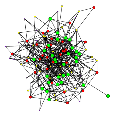
Figure 2: A Graphical Illustration of the Insurance Network of Nyakatoke

In the dataset there are 5 households that lack information on wealth and/or distance. We drop these observations, resulting in a sample size $N$ of 114. The total number of ordered household pairs is 12,882. Summary statistics for the dependent and explanatory variables used in our analysis are presented in Table 2.

Table 2: Empirical Application: Summary Statistics

Variable	Obs	Mean	Std. Dev.	Min	Max
link	12,882	0.0732	0.2606	0	1
$\left|\text{(ln) wealth difference}\right|$	12,882	1.0365	0.8228	0.0004	5.8898
($\ln$) distance	12,882	6.0553	0.7092	2.6672	7.4603
tie	12,882	0.4260	0.6123	0.0000	3.0000

Given the data structure, we should expect close to point identification because even though the tie variable is discrete, the other two regressors wealth and distance can be considered as being continuously distributed with a large conditional support. In addition, tie also has more than one point in its support given other variables. Thus, it is straightforward to verify that Assumption LABEL:as4prime2 is satisfied, leading to point identification of $\beta_{0}$.

5.2 Results and Discussion

We apply our two-stage estimator proposed in Section 3.3 to the Nyakatoke network data, where, similarly to the simulation studies, we use second degree splines to estimate $\rho_{i}$ and the adaptive grid search algorithm to find the minimizer of the criterion function $\widehat{Q}\left(\beta\right)$ on $\mathbb{\mathbb{S}}^{d-1}$.

Table 3: Empirical Application: Estimation Results

Variable	$\hat{\beta}^{m}$	$\left[\hat{\beta}^{l},\ \hat{\beta}^{u}\right]$
$\left|\text{(ln) wealth difference}\right|$	-0.1948	$\left[-0.1964,\ -0.1932\right]$
($\ln$) distance	-0.8036	$\left[-0.8043,\ -0.8029\right]$
tie	0.5619	$\left[0.5608,\ 0.5630\right]$

Table 3 summarizes our estimation results. The column of $\hat{\beta}^{m}$ corresponds to the center of the estimated rectangle

$$\widehat{\Xi}:=\times_{h=1}^{d}\left[\widehat{\beta}_{h}^{l},\ \widehat{\beta}_{h}^{u}\right],$$

where $\widehat{\beta}_{h}^{l}$ and $\widehat{\beta}_{h}^{u}$ represent the lower and upper bound of the estimated area (the set of minimizers of sample criterion function (22)) along each dimension $h=1,..,d$. We use $\hat{\beta}^{m}$ as the point estimator of the coefficients. While the scale of $\beta_{0}$ is unidentified, one can still compare the estimated coefficients with each other to obtain an idea about which variable affects the formation of the link more than the other.

The estimated coefficients for each variable conform well with economic intuition. The estimated set for wealth difference’s coefficient is $\left[-0.1964,-0.1932\right]$, which implies the more difference in wealth between two households, the lower likelihood they are connected. The estimated set for distance is $\left[-0.8043,-0.8029\right]$. It is natural that households rely more on neighbors for help than those who live farther away, thus neighbors are more likely to be connected. The estimated coefficient for tie falls in the positive range of $\left[0.5608,0.5630\right]$, consistent with the intuition that one would depend on support from family when negative shock occurs.

It is worth mentioning the estimated set $\hat{\Xi}$ is very tight in each dimension, with the maximum width $\max_{h=1,..,d}\left(\hat{\beta}_{h}^{u}-\hat{\beta}_{h}^{l}\right)$ equal to 0.0032 for wealth difference. Usually the discreteness in tie could make the estimated set wide, but our method is able to leverage the large support in wealth difference and distance. Once again, the relative magnitude and sign of the coefficient for tie are estimated in line with expectation despite of its discreteness. In summary, the empirical results show that our proposed estimator is able to generate economically intuitive estimates under NTU.

6 Conclusion

This paper considers a semiparametric model of dyadic network formation under nontransferable utilities, a natural and realistic micro-theoretical feature that translates into the lack of additive separability in econometric modeling. We show how a new methodology called logical differencing can be leveraged to cancel out the two-way fixed effects, which correspond to unobserved individual heterogeneity, without relying on arithmetic additivity. The key idea is to exploit the logical implication of weak multivariate monotonicity and use the intersection of mutually exclusive events on the unobserved fixed effects. It would be interesting to explore whether and how the idea of logical differencing, or more generally the use of fundamental logical operations, can be applied to other econometric settings.

The identified sets derived by our method under various support restrictions demonstrate that the proposed method is able to achieve accurate identified set despite of discreteness and boundedness in $Supp\left(X\right)$. Simulation results show that our method performs reasonably well with a relatively small sample size, and robust to various configurations. The empirical illustration using the real network data of Nyakatoke reveals that our method is able to capture the essence of the network formation process by generating estimates that conform well with economic intuition.

This paper also reveals several further research questions regarding dyadic network formation models under the NTU setting. First, given the observation that the NTU setting can capture “homophily effects” with respect to the unobserved heterogeneity (under log-concave error distributions) while imposing monotonicity in the unobserved heterogeneity, it is interesting to investigate whether one can differentiate homophily effects generated by “intrinsic preference” from assortativity effects generated by bilateral consent, NTU and log-concave errors. Second, admittedly the identifying restriction obtained in this paper becomes uninformative when we have antisymmetric pairwise observable characteristics. However, preliminary analysis based on an adaption of Gao (2020) to the NTU setting suggests that individual unobserved heterogeneity can be nonparametrically identified up to location and inter-quantile range normalizations. After the identification of individual unobserved heterogeneity terms ($A_{i}$), it becomes straightforward to identify the index parameter $\beta_{0}$ based on the observable characteristics, even in the presence of antisymmetric pairwise characteristics. However, consistent estimators of $A_{i}$ and $\beta_{0}$ in a semiparametric framework based on the identification strategy in Gao (2020) are still being developed. We thus leave these research questions to future work.

Acknowledgements

Wayne Gao is grateful to Xiaohong Chen and Peter C. B. Phillips for their advice and support while working on this paper during his PhD study at Yale University. Ming Li is grateful to Donald W. K. Andrews and Yuichi Kitamura for their advice and support while working on this paper during his PhD study at Yale University. We also thank Isaiah Andrews, Yann Bramoullé, Benjamin Connault, and Paul Goldsmith-Pinkham, as well as seminar and conference participants at Yale University, University of Arizona, University of Essex, the International Conference for Game Theory at Stony Brook University (2019), the Young Economist Symposium at Columbia University (2019), and the Latin American Meeting of the Econometric Society at Benemérita Universidad Autónoma de Puebla (2019) for their comments. All errors are our own.

Appendix

Appendix A Proofs

A.1 Proof of Lemma 2

Proof.

For notational simplicity, we denote $\Delta\left(x;x_{i},x_{j}\right)$ to be $w\left(x_{i},x\right)-w\left(x_{j},x\right)$ and write

$$\lambda\left(\overline{x},\underline{x};x_{i},x_{j};\beta\right)=\mathbf{\mathbbm{1}}\left\{\Delta\left(\overline{x};x_{i},x_{j}\right)^{{}^{\prime}}\beta\leq 0\right\}\mathbf{\mathbbm{1}}\left\{\Delta\left(\underline{x};x_{i},x_{j}\right)^{{}^{\prime}}\beta\geq 0\right\}.$$ (25)

Therefore, the event (20) is equivalent to $\left\{\Delta\left(\overline{x};x_{i},x_{j}\right)^{{}^{\prime}}\beta_{0}>0\right\}\cup\left\{\Delta\left(\underline{x};x_{i},x_{j}\right)^{{}^{\prime}}\beta_{0}<0\right\}$ and the event (21) is equivalent to $\left\{\Delta\left(\overline{x};x_{i},x_{j}\right)^{{}^{\prime}}\beta\leq 0\right\}\cap\left\{\Delta\left(\underline{x};x_{i},x_{j}\right)^{{}^{\prime}}\beta\geq 0\right\}$.

By Assumption 4, there exist $x_{i}$ and $x_{j}$ in $Supp\left(X_{i}\right)$ such that $\Delta\left(X_{k};x_{i},x_{j}\right)$ contains ${\bf 0}$ as an interior point, or in other words, contains all directions from the origin. Hence, given any directions $\beta_{0}$ and $\beta\neq\beta_{0}$ in $\mathbb{\mathbb{S}}^{d-1}$, there must exist some $\overline{x}\in Supp\left(X_{i}\right)$ such that

$$\Delta\left(\overline{x};x_{i},x_{j}\right){}^{{}^{\prime}}\beta_{0}>0\text{ and }\Delta\left(\overline{x};x_{i},x_{j}\right){}^{{}^{\prime}}\text{$\beta$}<0,$$ (26)

and some $\underline{x}\in Supp\left(X_{i}\right)$ such that

$$\Delta\left(\underline{x};x_{i},x_{j}\right){}^{{}^{\prime}}\beta_{0}<0\text{ and }\Delta\left(\underline{x};x_{i},x_{j}\right){}^{{}^{\prime}}\text{$\beta$}>0.$$ (27)

Since all the inequalities above are strict and $w$ is continuous (Assumption 3), there exists some $\epsilon>0$ such that, for every

$$\left(\tilde{x}_{i},\tilde{x}_{j},\tilde{\overline{x}},\tilde{\underline{x}}\right)\in\Upsilon:=B_{\epsilon}\left(x_{i}\right)\times B_{\epsilon}\left(x_{j}\right)\times B_{\epsilon}\left(\overline{x}\right)\times B_{\epsilon}\left(\underline{x}\right),$$

with $B_{\epsilon}\left(x\right)$ denoting the open ball of radius $\epsilon$ around $x$, we have

$$\Delta\left(\tilde{\overline{x}};\tilde{x}_{i},\tilde{x}_{j}\right){}^{{}^{\prime}}\beta_{0}>0\text{ and }\Delta\left(\tilde{\overline{x}};\tilde{x}_{i},\tilde{x}_{j}\right){}^{{}^{\prime}}\text{$\beta$}<0,$$

and

$$\Delta\left(\tilde{\underline{x}};\tilde{x}_{i},\tilde{x}_{j}\right){}^{{}^{\prime}}\beta_{0}<0\text{ and }\Delta\left(\tilde{\underline{x}};\tilde{x}_{i},\tilde{x}_{j}\right){}^{{}^{\prime}}\text{$\beta$}>0,$$

which imply (20) and (21). Since $x_{i},x_{j},\overline{x},\underline{x}$ all belong to $Supp\left(X_{i}\right)$, we have

$$\mathbb{P}\left(\left(X_{i},X_{j},X_{k},X_{l}\right)\in\Upsilon\right)>0,$$ (28)

when we randomly sample individuals $\left(i,j,k,l\right)$.

Now, fix any $\overline{a}\in Supp\left(A_{i}\right)$ and any $\left(\tilde{\overline{x}},\tilde{\underline{x}},\tilde{x}_{i},\tilde{x}_{j}\right)\in\Upsilon$. Since $\phi$ is strictly increasing in its first argument and continuous in all its arguments, the function $\psi_{\tilde{\overline{x}}}$

$$\psi_{\tilde{\overline{x}}}\left(w\left(\tilde{x}_{i},\tilde{\overline{x}}\right)^{{}^{\prime}}\beta_{0},a_{i}\right)=\int\phi\left(w\left(\tilde{x}_{i},\tilde{\overline{x}}\right)^{{}^{\prime}}\beta_{0},a_{i},A_{k}\right)d\mathbb{P}\left(\left.A_{k}\right|X_{k}=\tilde{\overline{x}}\right)$$

is also strictly increasing in its first argument and continuous in all its arguments. Hence,

$$\psi_{\tilde{\overline{x}}}\left(w\left(\tilde{x}_{i},\tilde{\overline{x}}\right)^{{}^{\prime}}\beta_{0},\overline{a}\right)-\psi_{\tilde{\overline{x}}}\left(w\left(\tilde{x}_{j},\tilde{\overline{x}}\right)^{{}^{\prime}}\beta_{0},\overline{a}\right)>0,$$

and similarly

$$\psi_{\tilde{\underline{x}}}\left(w\left(\tilde{x}_{i},\tilde{\underline{x}}\right)^{{}^{\prime}}\beta_{0},\overline{a}\right)-\psi_{\tilde{\underline{x}}}\left(w\left(\tilde{x}_{j},\tilde{\underline{x}}\right)^{{}^{\prime}}\beta_{0},\overline{a}\right)<0.$$

Furthermore, there must exist some $\epsilon>0$ such that, for any $a_{i},a_{j}\in\left[\overline{a}-\epsilon,\overline{a}+\epsilon\right]$, and any individuals $i,j$ with $\left(X_{i},A_{i}\right)=\left(\tilde{x}_{i},a_{i}\right)$ and $\left(X_{j},A_{j}\right)=$$\left(\tilde{x}_{j},a_{j}\right)$, we have

$$\rho_{i}\left(\tilde{\overline{x}}\right)-\rho_{j}\left(\tilde{\overline{x}}\right)=\psi_{\tilde{\overline{x}}}\left(w\left(\tilde{x}_{i},\tilde{\overline{x}}\right)^{{}^{\prime}}\beta_{0},a_{i}\right)-\psi_{\tilde{\overline{x}}}\left(w\left(\tilde{x}_{j},\tilde{\overline{x}}\right)^{{}^{\prime}}\beta_{0},a_{j}\right)>0$$

and

$$\rho_{i}\left(\tilde{\underline{x}}\right)-\rho_{j}\left(\tilde{\underline{x}}\right)=\psi_{\tilde{\underline{x}}}\left(w\left(\tilde{x}_{i},\tilde{\underline{x}}\right)^{{}^{\prime}}\beta_{0},a_{i}\right)-\psi_{\tilde{\underline{x}}}\left(w\left(\tilde{x}_{j},\tilde{\underline{x}}\right)^{{}^{\prime}}\beta_{0},a_{j}\right)<0,$$

which implies (19). Since

$$\overline{a}\in Supp\left(A_{i}\right)=Supp\left(\left.A_{i}\right|X_{i}=\tilde{x}_{i}\right)=Supp\left(\left.A_{j}\right|X_{j}=\tilde{x}_{j}\right)$$

by Assumption 5, we have

$$\mathbb{P}\left(\left.\tau_{ij}\left(\tilde{\overline{x}},\tilde{\underline{x}}\right)=1\right|X_{i}=\tilde{x}_{i},X_{j}=\tilde{x}_{j}\right)$$

$$>\ \mathbb{P}\left(\left.A_{i},A_{j}\in\left[\overline{a}-\epsilon,\overline{a}+\epsilon\right]\right|X_{i}=\tilde{x}_{i},X_{j}=\tilde{x}_{j}\right)>0.$$ (29)

Now, combining (28) and (29), we have

$$\mathbb{P}\left\{\eqref{eq:DNF_ID1},\eqref{eq:DNF_ID2}\text{ and }\eqref{eq:DNF_ID3}\text{ hold}\right\}$$

$$\geq\ \int_{\Upsilon}\mathbb{P}\left(\left.\tau_{ij}\left(X_{k},X_{l}\right)=1\right|X_{i}=\tilde{x}_{i},X_{j}=\tilde{x}_{j},X_{k}=\tilde{\overline{x}},X_{l}=\tilde{\underline{x}}\right)d\mathbb{P}\left(x_{i},x_{j},\overline{x},\underline{x}\right)>0$$

since the integrand is strictly positive on the set $\Upsilon$, which has strictly positive probability measure under $\mathbb{P}$. ∎

A.2 Proof of Theorem 1

Proof.

By Lemma 1, we have $\beta_{0}\in\arg\min_{\beta\in\text{$\mathbb{S}$}^{d-1}}Q(\beta)$ because $Q\left(\beta_{0}\right)=0\leq Q\left(\beta\right)$ by the construction of the population criterion $Q\left(\cdot\right)$. Furthermore, we have $\beta_{0}$ is the unique minimizer of $Q(\beta)$ because for any $\beta\neq\beta_{0}$, we have

$$Q\left(\beta\right) =\mathbb{E}\left[\lambda\left(X_{k},X_{l};X_{i},X_{j};\beta\right)\tau_{ij}\left(X_{k},X_{l}\right)\right]$$

$$\geq\mathbb{P}\left\{\eqref{eq:DNF_ID1},\eqref{eq:DNF_ID2}\text{ and }\eqref{eq:DNF_ID3}\text{ hold}\right\}>0,$$ (30)

by Lemma 2.

Now, for any $\beta\in\mathbb{\mathbb{S}}^{d-1}$, the function $g_{ij}\left(z,\beta\right):=\lambda\left(\overline{x},\underline{x};x_{i},x_{j};\beta\right)\tau_{ij}\left(\overline{x},\underline{x}\right)$ where $z:=\left(\overline{x},\underline{x};x_{i},x_{j}\right)$ is discontinuous in $\beta$ only on the (finite union of) hyperplanes defined by $\Delta(\overline{x};x_{i},x_{j})^{{}^{\prime}}\beta=0$ or $\Delta(\underline{x};x_{i},x_{j})^{{}^{\prime}}\beta=0$, which are probability zero events under Assumption 4. Moreover,

$$\mathbb{E}\sup_{\beta\in\mathbb{\mathbb{S}}^{d-1}}\left|g_{ij}\left(z,\beta\right)\right|\leq 1<\infty.$$ (31)

Hence, by Newey and McFadden (1994), $Q\left(\beta\right)$ is continuous, and, given that $\mathbb{\mathbb{S}}^{d-1}$ is compact, the desired result in Theorem 1 follows. ∎

A.3 Lemma 4 with Proof

We state and prove the following lemma that we use to prove Theorem 2.

Lemma 4 (Uniform Convergence of $\widehat{Q}_{n}^{\gamma}\left(\beta\right)$).

Under model (3) and Assumptions LABEL:as1prime, 2–7, we have

$$\sup_{\beta\in\text{$\mathbb{S}$}^{d-1}}\left|\widehat{Q}_{n}^{\gamma}\left(\beta\right)-Q^{\gamma}\left(\beta\right)\right|\overset{p}{\longrightarrow}0.$$

Proof.

For notational simplicity, we suppress the superscript $\gamma$ in this proof. Define the infeasible criterion $\widetilde{Q}_{n}\left(\beta\right)$ as

$$\widetilde{Q}_{n}\left(\beta\right):=\frac{\left(n-4\right)!}{n!}\sum_{1\leq i\neq j\neq k\neq l\leq n} \tau_{ij}^{\gamma}\left(X_{k},X_{l}\right)\lambda\left(X_{k},X_{l};X_{i},X_{j};\beta\right).$$ (32)

By triangular inequality, we have

$$\sup_{\beta\in\text{$\mathbb{S}$}^{d-1}}\left|\widehat{Q}_{n}\left(\beta\right)-Q\left(\beta\right)\right|\leq\sup_{\beta\in\text{$\mathbb{S}$}^{d-1}}\left|\widehat{Q}_{n}\left(\beta\right)-\widetilde{Q}\left(\beta\right)\right|+\sup_{\beta\in\text{$\mathbb{S}$}^{d-1}}\left|\widetilde{Q}\left(\beta\right)-Q\left(\beta\right)\right|.$$ (33)

We first show that $\sup_{\beta\in\text{$\mathbb{S}$}^{d-1}}\left|\widehat{Q}_{n}\left(\beta\right)-\widetilde{Q}\left(\beta\right)\right|=o_{p}\left(1\right)$. Since $\lambda$ only takes value in $\left\{0,1\right\}$, we have

$$\sup_{\beta\in\text{$\mathbb{S}$}^{d-1}}\left|\widehat{Q}_{n}\left(\beta\right)-\widetilde{Q}\left(\beta\right)\right|$$ (34)

$$= \ \frac{\left(n-4\right)!}{n!}\sum_{1\leq i\neq j\neq k\neq l\leq n}\sup_{\beta\in\text{$\mathbb{S}$}^{d-1}}\left|\lambda\left(X_{k},X_{l};X_{i},X_{j};\beta\right)\right|$$

$$\ \times\left|\gamma\left(\hat{\rho}_{i}(X_{k})-\hat{\rho}_{j}(X_{k})\right)\cdot\gamma\left(\hat{\rho}_{j}(X_{l})-\hat{\rho}_{i}(X_{l})\right)-\gamma\left(\rho_{i}(X_{k})-\rho_{j}(X_{k})\right)\cdot\gamma\left(\rho_{j}(X_{l})-\rho_{i}(X_{l})\right)\right|$$

$$\leq \ \frac{\left(n-4\right)!}{n!}\sum_{1\leq i\neq j\neq k\neq l\leq n}\left|\begin{array}[]{c}\gamma\left(\hat{\rho}_{i}(X_{k})-\hat{\rho}_{j}(X_{k})\right)\cdot\gamma\left(\hat{\rho}_{j}(X_{l})-\hat{\rho}_{i}(X_{l})\right)\\ -\gamma\left(\rho_{i}(X_{k})-\rho_{j}(X_{k})\right)\cdot\gamma\left(\rho_{j}(X_{l})-\rho_{i}(X_{l})\right)\end{array}\right|$$

$$\leq \ \frac{\left(n-4\right)!}{n!}\sum_{1\leq i\neq j\neq k\neq l\leq n}\left(\begin{array}[]{c}\left|\gamma\left(\hat{\rho}_{i}(X_{k})-\hat{\rho}_{j}(X_{k})\right)-\gamma\left(\rho_{i}(X_{k})-\rho_{j}(X_{k})\right)\right|\cdot\gamma\left(\rho_{j}(X_{l})-\rho_{i}(X_{l})\right)\\ +\gamma\left(\rho_{i}(X_{k})-\rho_{j}(X_{k})\right)\cdot\left|\gamma\left(\hat{\rho}_{j}(X_{l})-\hat{\rho}_{i}(X_{l})\right)-\gamma\left(\rho_{j}(X_{l})-\rho_{i}(X_{l})\right)\right|\\ +\left|\gamma\left(\hat{\rho}_{i}(X_{k})-\hat{\rho}_{j}(X_{k})\right)-\gamma\left(\rho_{i}(X_{k})-\rho_{j}(X_{k})\right)\right|\\ \cdot\left|\gamma\left(\hat{\rho}_{j}(X_{l})-\hat{\rho}_{i}(X_{l})\right)-\gamma\left(\rho_{j}(X_{l})-\rho_{i}(X_{l})\right)\right|\end{array}\right)$$

$$\leq \ C\cdot\frac{\left(n-4\right)!}{n!}\sum_{1\leq i\neq j\neq k\neq l\leq n}\left(\begin{array}[]{c}\left(\left|\hat{\rho}_{i}(X_{k})-\rho_{i}(X_{k})\right|+\left|\hat{\rho}_{j}(X_{k})-\rho_{j}(X_{k})\right|\right)\cdot\left|\rho_{j}(X_{l})-\rho_{i}(X_{l})\right|\\ +\left(\left|\hat{\rho}_{i}(X_{l})+\rho_{i}(X_{l})\right|+\left|\hat{\rho}_{j}(X_{l})-\rho_{j}(X_{l})\right|\right)\cdot\left|\rho_{i}(X_{k})-\rho_{j}(X_{k})\right|\\ +\left(\left|\hat{\rho}_{i}(X_{k})-\rho_{i}(X_{k})\right|+\left|\hat{\rho}_{j}(X_{k})-\rho_{j}(X_{k})\right|\right)\\ \cdot\left(\left|\hat{\rho}_{i}(X_{l})-\rho_{i}(X_{l})\right|+\left|\hat{\rho}_{j}(X_{l})-\rho_{j}(X_{l})\right|\right)\end{array}\right),$$

for some $C>0$, where the last inequality holds due to Lipschitz-continuity of $\gamma$ in Assumption 7.

Recall that $\rho_{i}$ as a function is identified by $\left(x_{i},a_{i}\right)$ through

$$\rho_{i}\left(x\right)=\int\phi\left(w\left(x,x_{i}\right)^{{}^{\prime}}\beta_{0},a_{i},A_{k}\right)\mathbb{P}\left(\left.A_{k}\right|X_{k}=x\right).$$

We write the $L_{2}\left(\mathbb{P}_{X}\right)$ norm of $\rho_{i}$ to mean

$$\left\|\rho_{i}\right\|:=\sqrt{\int\rho_{i}^{2}\left(x\right)d\mathbb{P}\left(X_{k}=x\right)}$$

and use the subscripts of $\mathbb{E}$ to denote expectation over variables indexed by those subscripts, e.g.,

$$\mathbb{E}_{i}\left\|\rho_{i}\right\|:=\int\left\|\rho_{i}\right\|d\mathbb{P}\left(X_{i}=x_{i},A_{i}=a_{i}\right).$$

Then, by (34), we have

$$\ \mathbb{E}\sup_{\beta\in\text{$\mathbb{S}$}^{d-1}}\left|\widehat{Q}_{n}\left(\beta\right)-\widetilde{Q}\left(\beta\right)\right|\cdot\frac{1}{C}$$

$$\leq \ \mathbb{E}_{ijkl}\left[\left(\left|\hat{\rho}_{i}(X_{k})-\rho_{i}(X_{k})\right|+\left|\hat{\rho}_{j}(X_{k})-\rho_{j}(X_{k})\right|\right)\cdot\left|\rho_{j}(X_{l})-\rho_{i}(X_{l})\right|\right]$$

$$\ +\mathbb{E}_{ijkl}\left[\left(\left|\hat{\rho}_{i}(X_{l})-\rho_{i}(X_{l})\right|+\left|\hat{\rho}_{j}(X_{l})-\rho_{j}(X_{l})\right|\right)\cdot\left|\rho_{i}(X_{k})-\rho_{j}(X_{k})\right|\right]$$

$$\ +\mathbb{E}_{ijkl}\left[\left(\left|\hat{\rho}_{i}(X_{k})-\rho_{i}(X_{k})\right|+\left|\hat{\rho}_{j}(X_{k})-\rho_{j}(X_{k})\right|\right)\left(\left|\hat{\rho}_{i}(X_{l})+\rho_{i}(X_{l})\right|+\left|\hat{\rho}_{j}(X_{l})-\rho_{j}(X_{l})\right|\right)\right]$$

$$= \ 2\mathbb{E}_{ijkl}\left|\hat{\rho}_{i}(X_{k})-\rho_{i}(X_{k})\right|\left|\rho_{j}(X_{l})-\rho_{i}(X_{l})\right|+2\mathbb{E}_{ijkl}\left|\hat{\rho}_{j}(X_{k})-\rho_{j}(X_{k})\right|\left|\rho_{j}(X_{l})-\rho_{i}(X_{l})\right|$$

$$\ +\mathbb{E}_{ik}\left|\hat{\rho}_{i}(X_{k})-\rho_{i}(X_{k})\right|^{2}+\mathbb{E}_{jk}\left|\hat{\rho}_{j}(X_{k})-\rho_{j}(X_{k})\right|^{2}+\mathbb{E}_{ik}\left|\hat{\rho}_{i}(X_{k})-\rho_{i}(X_{k})\right|\mathbb{E}_{jl}\left|\hat{\rho}_{j}(X_{l})-\rho_{j}(X_{l})\right|$$

$$\leq \ 2\mathbb{E}_{ik}\left|\hat{\rho}_{i}(X_{k})-\rho_{i}(X_{k})\right|+2\mathbb{E}_{jk}\left|\hat{\rho}_{j}(X_{k})-\rho_{j}(X_{k})\right|$$

$$\ +\mathbb{E}_{ik}\left|\hat{\rho}_{i}(X_{k})-\rho_{i}(X_{k})\right|^{2}+\mathbb{E}_{jk}\left|\hat{\rho}_{j}(X_{k})-\rho_{j}(X_{k})\right|^{2}+\mathbb{E}_{ik}\left|\hat{\rho}_{i}(X_{k})-\rho_{i}(X_{k})\right|\mathbb{E}_{jl}\left|\hat{\rho}_{j}(X_{l})-\rho_{j}(X_{l})\right|$$

$$\leq \ 4\mathbb{E}_{i}\left\|\hat{\rho}_{i}-\rho_{i}\right\|+2\mathbb{E}_{i}\left\|\hat{\rho}_{i}-\rho_{i}\right\|^{2}+\mathbb{E}_{i}\left\|\hat{\rho}_{i}-\rho_{i}\right\|\cdot\mathbb{E}_{j}\left\|\hat{\rho}_{j}-\rho_{j}\right\|$$

$$= \ 4\mathbb{E}_{i}\left[o_{p}\left(1\right)\right]+2\mathbb{E}_{i}\left[\left(o_{p}\left(1\right)\right)^{2}\right]+\left(\mathbb{E}_{i}\left[o_{p}\left(1\right)\right]\right)^{2}$$

$$= \ o_{p}\left(1\right)$$

where the second last inequality follows from the observation that $\left|\rho_{j}-\rho_{i}\right|\leq 1$, while the last inequality follows from the Cauchy–Schwarz inequality, and the second last equality follows from $\left\|\hat{\rho}_{i}-\rho_{i}\right\|=o_{p}\left(1\right)$ by the $L_{2}\left(\mathbb{P}_{X}\right)$-consistency of $\hat{\rho}_{i}$ for each $i$. Finally, by the Markov inequality, we have

$$\sup_{\beta\in\text{$\mathbb{S}$}^{d-1}}\left|\widehat{Q}_{n}\left(\beta\right)-\widetilde{Q}\left(\beta\right)\right|=o_{p}\left(1\right).$$ (35)

Next, we show

$$\sup_{\beta\in\text{$\mathbb{S}$}^{d-1}}\left|\widetilde{Q}_{n}\left(\beta\right)-Q\left(\beta\right)\right|=o_{p}\left(1\right).$$

Clearly, $\left\{\widetilde{Q}_{n}\left(\beta\right)-Q\left(\beta\right):\beta\in\mathbb{S}^{d-1}\right\}$ is a centered U-process of order $4$, and we apply the results in Arcones and Giné (1993) for U-statistic empirical processes.

To start, we know that the collection of halfspaces $x^{{}^{\prime}}\beta\geq 0$ across $\beta\in\mathbb{\mathbb{S}}^{d-1}$ is a VC class of functions with VC dimension $d+2$, by Problem 14 in Section 6 of Van Der Vaart and Wellner (1996, VW thereafter). Furthermore, the intersection of VC classes remains VC by Lemma 2.6.17(ii) of VW. Hence, $\left\{\lambda\left(\cdot,\beta\right):\beta\in\mathbb{\mathbb{S}}^{d-1}\right\}$ is a VC-subgraph class of functions. Since $\left\{\lambda\left(\cdot,\beta\right):\beta\in\mathbb{\mathbb{S}}^{d-1}\right\}$ has a constant envelope function 1, which trivially has finite expectation. By Corollary 3.3 of Arcones and Giné (1993), $\left\{\lambda\left(\cdot,\beta\right):\beta\in\mathbb{\mathbb{S}}^{d-1}\right\}$ is a Glivenko-Cantelli class,

Next, by VW Corollary 2.7.2 that the bracketing number

$$\mathscr{N}_{[]}\left(\epsilon,{\cal C}_{M}^{\left\lfloor d/2\right\rfloor+1}\left(Supp\left(X_{i}\right)\right),\left\|\cdot\right\|_{1,\mathbb{P}}\right)<\infty$$

for every $\epsilon>0$. Hence, by Corollary 3.3 of Arcones and Giné (1993), we know that ${\cal C}_{M}^{\left\lfloor d/2\right\rfloor+1}\left(Supp\left(X_{i}\right)\right)$ is also Glivenko-Cantelli.

Now, since the mapping

$$\left(\rho_{i},\rho_{j},\lambda\right)\mapsto\gamma\left(\rho_{i}-\rho_{j}\right)\gamma\left(\rho_{j}-\rho_{i}\right)\lambda\left(\cdot,\beta\right)$$

is continuous in all its arguments, by Theorem 3 of Van Der Vaart and Wellner (2000), we know that

$$\left\{\gamma\left(\rho_{i}-\rho_{j}\right)\gamma\left(\rho_{j}-\rho_{i}\right)\lambda\left(\cdot,\beta\right):\rho_{i},\rho_{j}\in{\cal C}_{M}^{\left\lfloor d/2\right\rfloor+1}\left(Supp\left(X_{i}\right)\right),\beta\in\mathbb{\mathbb{S}}^{d-1}\right\}$$

is also Glivenko-Cantelli, i.e.,

$$\sup_{\beta\in\text{$\mathbb{S}$}^{d-1}}\left|\widetilde{Q}_{n}\left(\beta\right)-Q\left(\beta\right)\right|\overset{p}{\longrightarrow}0.$$ (36)

Combining (35) and (36), we have

$$\sup_{\beta\in\text{$\mathbb{S}$}^{d-1}}\left|\widehat{Q}_{n}\left(\beta\right)-Q\left(\beta\right)\right|\overset{p}{\longrightarrow}0.$$ (37)

∎

A.4 Proof of Theorem 2

Proof.

By the standard theory of M-estimation, say, Theorem 5.7 of Van der Vaart (2000), the conclusion of Theorem 2 follows from Theorem 1 (clean point identification) and Lemma 4 (uniform convergence of sample criterion). ∎

Appendix B Point Identification with a Special Covariate

Assumption 4^′′ Suppose that:

• $w_{h}\left(\overline{x},\underline{x}\right):=\left|\overline{x}_{h}-\underline{x}_{h}\right|$ for every coordinate $h$;

• $\beta_{0,1}\neq 0$.

• the support of $X_{i,1}$ given all other coordinates $X_{i,-1}$ is the whole real line $\mathbb{R}$.

• there exist two distinct values $\overline{x}_{h},\underline{x}_{h}\in\mathbb{R}$ for each coordinate $h\in\left\{2,...,d\right\}$ such that $\vartimes_{h=2}^{d}\left\{\overline{x}_{h},\underline{x}_{h}\right\}\subseteq Supp\left(X_{i,-1}\right).$

Assumption LABEL:as4prime2 is very similar to the corresponding set of assumptions imposed for maximum-score estimators a la Horowitz (1992), with the exception that Assumption LABEL:as4prime2(iv) is stronger than the corresponding condition in Horowitz (1992), which only requires that the support of $X_{i}$ is not contained in any proper linear subspace of $\mathbb{R}^{d}$. Nevertheless, we regard Assumption LABEL:as4prime2(iv) as a very mild requirement: it essentially requires that the conditional support of each coordinate of $X_{i,-1}$ does not degenerate to a singleton, at least in some part of $Supp\left(X_{i,-1}\right)$. Assumption LABEL:as4prime2(iv) effectively enables us to vary one discrete coordinate while holding the other coordinates in $X_{i,-1}$ fixed. Even though this condition is stronger than necessary, it drastically simplifies the proof of point identification below.

To see the intuition through a more concrete example, suppose $X_{i}$ is two-dimensional and $\beta_{0}=\left(1,1\right)^{{}^{\prime}}$. Then, to differentiate $\beta_{0}$ from $\beta=\left(1,-1\right)^{{}^{\prime}}$, we need to find in-support $\left(X_{i},X_{j},X_{k},X_{l}\right)$ such that both

$$\text{sgn}\left\{\left(W_{ik}-W_{jk}\right)^{{}^{\prime}}\beta_{0}\right\} \neq\text{sgn}\left\{\left(W_{ik}-W_{jk}\right)^{{}^{\prime}}\beta\right\}\text{ and }$$

$$\text{sgn}\left\{\left(W_{il}-W_{jl}\right)^{{}^{\prime}}\beta_{0}\right\} \neq\text{sgn}\left\{\left(W_{il}-W_{jl}\right)^{{}^{\prime}}\beta\right\}$$

are satisfied in order to have (19), (20) and (21) occur simultaneously with strictly positive probability. But this is not possible if the second (discrete) dimension of $X$ is the same for all individuals, since $\beta_{0}^{\left(1\right)}=\beta^{\left(1\right)}=1$ and the only way to flip the sign is to vary the second coordinate of $X$ for each individual. The general argument will be made clearer in the proof of Lemma LABEL:lem2prime2.

Given Assumption LABEL:as4prime2(ii), it is standard to proceed with a different normalization from the unit sphere $\mathbb{\mathbb{S}}^{d-1}$ in the main text:

$$\beta_{0}\in{\cal B}:=\left\{1,-1\right\}\times\mathbb{R}^{d-1}.$$

Lemma 2^′′ Under model (3), Assumptions LABEL:as1prime, 2, 3, LABEL:as4prime2, and 5, for each $\beta\in{\cal B}\backslash\left\{\beta_{0}\right\}$, (19), (20) and (21) occur simultaneously with strictly positive probability.

Proof.

Take any $\beta\in{\cal B}\backslash\left\{\beta_{0}\right\}$. We consider three separate cases:

Case 1: $\beta_{1}=\beta_{0,1}=1$.

In this case, there exists some coordinate $h\neq 1$ such that $\beta_{h}\neq\beta_{0,h}$. Set

$$\underline{x}_{-1} :=\left(\underline{x}_{2},..,\underline{x}_{h}\right)$$

$$\hat{x}_{-1} :=\underline{x}_{-1}+\left(\overline{x}_{h}-\underline{x}_{h}\right)e_{h}$$

where $e_{h}$ denotes the elementary vector with 1 for coordinate $h$ and $0$ elsewhere. By Assumption LABEL:as4prime2(iv), $\underline{x}_{-1},\hat{x}_{-1}\in Supp\left(X_{i,-1}\right)$. Moreover

$$w_{-1}\left(\hat{x}_{-1},\underline{x}_{-1}\right)-w_{-1}\left(\underline{x}_{-1},\underline{x}_{-1}\right)=\left|\overline{x}_{h}-\underline{x}_{h}\right|e_{h}$$

Now, writing

$$z :=\left|\overline{x}_{h}-\underline{x}_{h}\right|\beta_{0,h}\in\mathbb{R},$$

$$\delta :=\left|\overline{x}_{h}-\underline{x}_{h}\right|\left(\beta_{0,h}-\beta_{h}\right)\neq 0,$$

we have

$$\left(w_{-1}\left(\hat{x}_{-1},\underline{x}_{-1}\right)-w_{-1}\left(\underline{x}_{-1},\underline{x}_{-1}\right)\right)^{{}^{\prime}}\beta_{-1}=\left|\overline{x}_{h}-\underline{x}_{h}\right|\beta_{h}=z-\delta$$

$$\neq\ z=\left|\overline{x}_{h}-\underline{x}_{h}\right|\beta_{0,h}=\left(w_{-1}\left(\hat{x}_{-1},\underline{x}_{-1}\right)-w_{-1}\left(\underline{x}_{-1},\underline{x}_{-1}\right)\right)^{{}^{\prime}}\beta_{0,-1}$$

and

$$\left(w_{-1}\left(\hat{x}_{-1},\hat{x}_{-1}\right)-w_{-1}\left(\underline{x}_{-1},\hat{x}_{-1}\right)\right)^{{}^{\prime}}\beta_{-1}=-\left|\overline{x}_{h}-\underline{x}_{h}\right|\beta_{h}=-z+\delta$$

$$\neq\ -z=-\left|\overline{x}_{h}-\underline{x}_{h}\right|\beta_{0,h}=\left(w_{-1}\left(\hat{x}_{-1},\hat{x}_{-1}\right)-w_{-1}\left(\underline{x}_{-1},\hat{x}_{-1}\right)\right)^{{}^{\prime}}\beta_{0,-1}$$

Now, by Assumption LABEL:as4prime2(iii), we can set

$$\hat{x} :=\left(\left[\frac{1}{2}\delta-z\right]_{+},\ \hat{x}_{-1}\right)\in Supp\left(X_{i}\right),$$

$$\check{x} :=\left(\left[z-\frac{1}{2}\delta\right]_{+},\ \underline{x}_{-1}\right)\in Supp\left(X_{i}\right),$$

$$\tilde{x} :=\left(0,\ \underline{x}_{-1}\right)\in Supp\left(X_{i}\right),$$

$$\mathring{x} :=\left(\left[\frac{1}{2}\delta-z\right]_{+}+\left[z-\frac{1}{2}\delta\right]_{+},\ \hat{x}_{-1}\right)\in Supp\left(X_{i}\right).$$

so that

$$\Delta\left(\tilde{x};\hat{x},\check{x}\right){}^{{}^{\prime}}\beta_{0} =\left(w\left(\hat{x},\tilde{x}\right)-w\left(\check{x},\tilde{x}\right)\right)^{{}^{\prime}}\beta_{0}$$

$$=\left|\hat{x}_{1}\right|-\left|\check{x}_{1}\right|+\left|\overline{x}_{h}-\underline{x}_{h}\right|\beta_{0,h}$$

$$=\left(\frac{1}{2}\delta-z\right)+z=\frac{1}{2}\delta,$$

$$\Delta\left(\tilde{x};\hat{x},\check{x}\right){}^{{}^{\prime}}\beta =\left(w\left(\hat{x},\tilde{x}\right)-w\left(\check{x},\tilde{x}\right)\right)^{{}^{\prime}}\beta$$

$$=\left(\left|\hat{x}_{1}\right|-\left|\check{x}_{1}\right|\right)+\left|\overline{x}_{h}-\underline{x}_{h}\right|\beta_{h}$$

$$=\left(\frac{1}{2}\delta-z\right)+\left(z-\delta\right)=-\frac{1}{2}\delta,$$ (38)

$$\Delta\left(\mathring{x};\hat{x},\check{x}\right){}^{{}^{\prime}}\beta_{0} =\left(w\left(\hat{x},\mathring{x}\right)-w\left(\check{x},\mathring{x}\right)\right)^{{}^{\prime}}\beta_{0}$$

$$=\left(\left|\hat{x}_{1}-\mathring{x}_{1}\right|-\left|\check{x}_{1}-\mathring{x}_{1}\right|\right)-\left|\overline{x}_{h}-\underline{x}_{h}\right|\beta_{0,h}$$

$$=z-\frac{1}{2}\delta-z=-\frac{1}{2}\delta,$$

$$\Delta\left(\mathring{x};\hat{x},\check{x}\right){}^{{}^{\prime}}\beta =\left(w\left(\hat{x},\mathring{x}\right)-w\left(\check{x},\mathring{x}\right)\right)^{{}^{\prime}}\beta>0$$

$$=\left(\left|\hat{x}_{1}-\mathring{x}_{1}\right|-\left|\check{x}_{1}-\mathring{x}_{1}\right|\right)-\left|\overline{x}_{h}-\underline{x}_{h}\right|\beta_{h}$$

$$=z-\frac{1}{2}\delta-z+\delta=\frac{1}{2}\delta,$$

which exactly correspond to the inequalities (26) and (27) in the proof of Lemma 2, both of the form

$$\text{sgn}\left(\Delta\left(\tilde{x};\hat{x},\check{x}\right){}^{{}^{\prime}}\beta_{0}\right)=\text{sgn}\left(\Delta\left(\mathring{x};\hat{x},\check{x}\right){}^{{}^{\prime}}\beta\right)\neq\text{sgn}\left(\Delta\left(\mathring{x};\hat{x},\check{x}\right){}^{{}^{\prime}}\beta_{0}\right)=\text{sgn}\left(\Delta\left(\tilde{x};\hat{x},\check{x}\right){}^{{}^{\prime}}\beta\right)$$

Again, since all the inequalities in (38) are strict, they continue to hold for points in sufficiently small open balls around $\hat{x},\check{x},\tilde{x},\mathring{x}$. And since $\hat{x},\check{x},\tilde{x},\mathring{x}$ are all taken from $Supp\left(X_{i}\right)$, any small open balls around them have strictly positive probability measures. The rest of the proof is exactly the same as in the proof of Lemma 2.

Case 2: $\beta_{1}=\beta_{0,1}=-1$.

This case can be handled in the same way as in Case 1, with appropriate changes of signs.

Case 3: $\beta_{1}\neq\beta_{0,1}$.

In this case, we can take any point $\underline{x}_{-1}\in Supp\left(X_{i,-1}\right)$ and set

$$\hat{x} :=\left(\left[\beta_{0,1}\right]_{+},\ \underline{x}_{-1}\right)\in Supp\left(X_{i}\right),$$

$$\check{x} :=\left(\left[-\beta_{0,1}\right]_{+},\ \underline{x}_{-1}\right)\in Supp\left(X_{i}\right),$$

$$\tilde{x} :=\left(0,\ \underline{x}_{-1}\right)\in Supp\left(X_{i}\right),$$

$$\mathring{x} :=\left(\left[\beta_{0,1}\right]_{+}+\left[-\beta_{0,1}\right]_{+},\ \underline{x}_{-1}\right)\in Supp\left(X_{i}\right),$$

so that

$$\Delta\left(\tilde{x};\hat{x},\check{x}\right){}^{{}^{\prime}}\beta_{0} =\left(\left|\hat{x}_{1}\right|-\left|\check{x}_{1}\right|\right)\beta_{0,1}=1>0,$$

$$\Delta\left(\tilde{x};\hat{x},\check{x}\right){}^{{}^{\prime}}\beta =\left(\left|\hat{x}_{1}\right|-\left|\check{x}_{1}\right|\right)\beta_{1}=-1<0,$$

$$\Delta\left(\mathring{x};\hat{x},\check{x}\right){}^{{}^{\prime}}\beta_{0} =\left(\left|\hat{x}_{1}-\mathring{x}_{1}\right|-\left|\check{x}_{1}-\mathring{x}_{1}\right|\right)\beta_{0,1}=-1<0,$$

$$\Delta\left(\mathring{x};\hat{x},\check{x}\right){}^{{}^{\prime}}\beta =\left(\left|\hat{x}_{1}-\mathring{x}_{1}\right|-\left|\check{x}_{1}-\mathring{x}_{1}\right|\right)\beta_{1}=1>0,$$

which again exactly correspond to the inequalities (26) and (27). The rest of the proof is exactly the same as in the proof of Lemma 2. ∎

Appendix C Asymmetry of Pairwise Observable Characteristics

So far we have been focusing on the case with symmetric pairwise observable characteristics, i.e.,

$$w\left(X_{i},X_{j}\right)\equiv w\left(X_{j},X_{i}\right).$$

In this section, we briefly discuss how our method can be adapted to accommodate asymmetric pairwise observable characteristics.

As in Remark 1, consider the adapted model (6):

$$\mathbb{E}\left[\left.D_{ij}\right|X_{i},X_{j},A_{i},A_{j}\right]=\phi\left(w\left(X_{i},X_{j}\right)^{{}^{\prime}}\beta_{0},w\left(X_{j},X_{i}\right)^{{}^{\prime}}\beta_{0},A_{i},A_{j}\right)$$ (39)

where $w$ needs not be symmetric with respect to its two vector arguments and $\phi:\mathbb{R}^{4}\to\mathbb{R}$ is required to be monotone in all its four arguments.

The technique of logical differencing still applies in the exactly same way as before. Specifically, the event $\left\{\rho_{\overline{i}}\left(\overline{x}\right)>\rho_{\overline{j}}\left(\overline{x}\right)\right\}$ implies that

$$\left\{w\left(X_{\overline{i}},\overline{x}\right)^{{}^{\prime}}\beta_{0}>w\left(X_{\overline{j}},\overline{x}\right)^{{}^{\prime}}\beta_{0}\right\}\text{ OR }\left\{w\left(\overline{x},X_{\overline{i}}\right)^{{}^{\prime}}\beta_{0}>w\left(\overline{x},X_{\overline{j}}\right)^{{}^{\prime}}\beta_{0}\right\}\text{ OR }\left\{A_{\overline{i}}>A_{\overline{j}}\right\},$$

while the event $\left\{\rho_{\overline{i}}\left(\underline{x}\right)<\rho_{\overline{j}}\left(\underline{x}\right)\right\}$ implies that

$$\left\{w\left(X_{\overline{i}},\underline{x}\right)^{{}^{\prime}}\beta_{0}<w\left(X_{\overline{j}},\underline{x}\right)^{{}^{\prime}}\beta_{0}\right\}\text{ OR }\left\{w\left(\underline{x},X_{\overline{i}}\right)^{{}^{\prime}}\beta_{0}<w\left(\underline{x},X_{\overline{j}}\right)^{{}^{\prime}}\beta_{0}\right\}\text{ OR }\left\{A_{\overline{i}}<A_{\overline{j}}\right\}.$$

The joint occurrence of $\left\{\rho_{\overline{i}}\left(\overline{x}\right)>\rho_{\overline{j}}\left(\overline{x}\right)\right\}$ and $\left\{\rho_{\overline{i}}\left(\underline{x}\right)<\rho_{\overline{j}}\left(\underline{x}\right)\right\}$ now implies that

$$\left\{w\left(X_{\overline{i}},\overline{x}\right)^{{}^{\prime}}\beta_{0}>w\left(X_{\overline{j}},\overline{x}\right)^{{}^{\prime}}\beta_{0}\right\}\text{ OR }\left\{w\left(\overline{x},X_{\overline{i}}\right)^{{}^{\prime}}\beta_{0}>w\left(\overline{x},X_{\overline{j}}\right)^{{}^{\prime}}\beta_{0}\right\}$$

OR $$\left\{w\left(X_{\overline{i}},\underline{x}\right)^{{}^{\prime}}\beta_{0}<w\left(X_{\overline{j}},\underline{x}\right)^{{}^{\prime}}\beta_{0}\right\}\text{ OR }\left\{w\left(\underline{x},X_{\overline{i}}\right)^{{}^{\prime}}\beta_{0}<w\left(\underline{x},X_{\overline{j}}\right)^{{}^{\prime}}\beta_{0}\right\},$$ (40)

which is in general “less restrictive” than the corresponding identifying restriction in Lemma 1.

In particular, in the extreme case where $w$ is antisymmetric in the sense of

$$w\left(X_{i},X_{j}\right)\equiv-w\left(X_{j},X_{i}\right),$$

the identifying restriction on the RHS of

$$\left\{w\left(X_{\overline{i}},\overline{x}\right)^{{}^{\prime}}\beta_{0}>w\left(X_{\overline{j}},\overline{x}\right)^{{}^{\prime}}\beta_{0}\right\}\text{ OR }\left\{w\left(\overline{x},X_{\overline{i}}\right)^{{}^{\prime}}\beta_{0}>w\left(\overline{x},X_{\overline{j}}\right)^{{}^{\prime}}\beta_{0}\right\}$$

becomes

$$\left\{w\left(X_{\overline{i}},\overline{x}\right)^{{}^{\prime}}\beta_{0}\neq w\left(X_{\overline{j}},\overline{x}\right)^{{}^{\prime}}\beta_{0}\right\},$$

which can be generically true and thus becomes (almost) trivial.

Correspondingly, Assumption 4 needs to be strengthened for point identification:

Assumption (3a).

There exist a pair of $\overline{x},\underline{x}$, both of which lie in the support of $Supp\left(X_{i}\right)$, such that

$$Supp\left(w\left(\overline{x},X_{i}\right)-w\left(\underline{x},X_{i}\right)\right)\cap Supp\left(w\left(X_{i},\overline{x}\right)-w\left(X_{i},\underline{x}\right)\right)$$

contains all directions in $\mathbb{R}^{d}$.

Clearly, the case of antisymmetric $w$ is ruled out by Assumption 3a. Assumption Assumption ensures that, for any $\beta\neq\beta_{0}$, there exist in-support $x_{i}$ and $x_{j}$ such that

$$\left\{w\left(x_{i},X_{k}\right)^{{}^{\prime}}\beta_{0}>w\left(x_{j},X_{k}\right)^{{}^{\prime}}\beta_{0}\right\}\text{ AND }\left\{w\left(x_{i},X_{l}\right)^{{}^{\prime}}\beta_{0}<w\left(x_{j},X_{l}\right)^{{}^{\prime}}\beta_{0}\right\}$$

AND $$\left\{w\left(X_{k},x_{i}\right)^{{}^{\prime}}\beta_{0}>w\left(X_{k},x_{j}\right)^{{}^{\prime}}\beta_{0}\right\}\text{ AND }\left\{w\left(X_{l},x_{i}\right)^{{}^{\prime}}\beta_{0}<w\left(X_{l},x_{j}\right)^{{}^{\prime}}\beta_{0}\right\}$$ (41)

and

$$\left\{w\left(x_{i},X_{k}\right)^{{}^{\prime}}\beta\leq w\left(x_{j},X_{k}\right)^{{}^{\prime}}\beta\right\}\text{ AND }\left\{w\left(x_{i},X_{l}\right)^{{}^{\prime}}\beta\geq w\left(x_{j},X_{l}\right)^{{}^{\prime}}\beta\right\}$$

AND $$\left\{w\left(X_{k},x_{i}\right)^{{}^{\prime}}\beta\leq w\left(X_{k},x_{j}\right)^{{}^{\prime}}\beta\right\}\text{ AND }\left\{w\left(X_{l},x_{i}\right)^{{}^{\prime}}\beta\geq w\left(X_{l},x_{j}\right)^{{}^{\prime}}\beta\right\}$$ (42)

occur simultaneously with strictly positive probability. (41) and (42) are sufficient for $\left\{\rho_{\overline{i}}\left(\overline{x}\right)>\rho_{\overline{j}}\left(\overline{x}\right)\right\}$ and $\left\{\rho_{\overline{i}}\left(\underline{x}\right)<\rho_{\overline{j}}\left(\underline{x}\right)\right\}$ to occur simultaneously under the maintained assumption on the support of $A_{i}$. It thus can guarantee point identification of $\beta_{0}$.

The estimator can be correspondingly adapted in an obvious manner.

Appendix D Additional Simulation Results

D.1 Results Varying $N$ and $d$

In this section, we vary the number of individuals $N$ and $\beta_{0}$’s dimension $d$ to examine how robust our method is against these variations. We investigate the performance when $N=50,100,200$ and $d=3,4$, respectively. We maintain the symmetry in $w\left(\cdot,\cdot\right)$ and other distributional assumptions as in baseline setup. $M$, the number of $\left(i,j\right)$ pairs used to evaluate objective function, is set to be 1,000 in all simulations. Note that one could make $M$ larger for larger $N$ to better capture the more information available from the increase in $N$. In this sense, our results are conservative below. Results are summarized in Table 4.

Table 4: Results Varying $N$ and $d$

$d=3$	rMSE	MND	MMAD	$d=4$	rMSE	MND	MMAD
$N=50$	0.0839	0.0724	0.0051	$N=50$	0.1119	0.1030	0.0091
$N=100$	0.0488	0.0417	0.0053	$N=100$	0.0692	0.0647	0.0038
$N=200$	0.0334	0.029	0.0043	$N=200$	0.0543	0.0523	0.0038

The left part of Table 4 shows the performance of our estimator when $N$ changes and $d$ is fixed at 3. When $N$ increases, rMSE, MND and sum of absolute bias all show moderate decline in magnitude, indicating the performance is improving. Similar pattern is also observed for $d=4$. This is intuitive because with more individuals in the sample, one can achieve more accurate estimation of $\rho_{i}\left(\cdot\right)$ and calculation of $\widehat{Q}\left(\beta\right)$. Moreover, we can see even with a relatively small sample size of $N=50$, the rMSE is 0.0839 when $d=3$ and 0.1119 when $d=4$, showing that our method is informative and accurate. When $N=200$, the performance is very good, with rMSE being as small as 0.0334 and 0.0543 for $d=3$ and $d=4$, respectively. When we fix $N$ and compare between $d=3$ and $d=4$, it is clear the increase in $d$ adversely affects the performance of our estimator, with rMSE and MND increasing for each $N$. Overall, Table 4 provides evidence that our method is able to estimate $\beta_{0}$ accurately even with a small sample size.

D.2 Results Varying $corr$

Correlation between observable characteristics $X$ and unobservable fixed effect $A$ is important in network formation models. We show how our estimator performs when the correlation between $X$ and $A$ varies. Recall that we constructed $A_{i}$ as

$$A_{i}=corr\times X_{i,1}+\left(1-corr\right)\times\xi_{i}.$$ (43)

We maintain the baseline DGP for $\left(D,X,w,A,\epsilon,\xi,\beta_{0}\right)$ as well as $\left(N,M,d\right)$ as in Section 4.2 and vary $corr$ from 0.20 to 0.90. Results are summarized in Table 5.

Table 5: Results Varying $corr$

$corr$	rMSE	MND	MMAD
0.20	0.0488	0.0417	0.0053
0.50	0.0489	0.0435	0.0186
0.75	0.0763	0.0690	0.0506
0.90	0.1010	0.0951	0.0743

It can be seen from Table 5 that even though increase in $corr$ adversely affects the performance of our estimator, the magnitude of the impact is relatively small. For example, rMSE only increases from 0.0488 to 0.1010 when $corr$ increase dramatically from 0.20 to 0.90. Similar pattern is also observed using other performance metrics. Therefore, our estimator is robust against correlation between $X$ and $A$.

D.3 Results under Asymmetric Pairwise Observable Characteristics

Following the theoretical analysis in Section C, we investigate how our method works when $w\left(X_{i},X_{j}\right)$ is asymmetric in $\left(X_{i},X_{j}\right)$, i.e., $W_{ij,h}:=w_{h}\left(X_{i},X_{j}\right)\neq w_{h}\left(X_{j},X_{i}\right)=:W_{ji,h}$ for at least one coordinate $h\in\left\{1,..,d\right\}$. To do so, we let $W_{ij,d}=\left|2X_{i,d}-X_{j,d}\right|\times\left(2/3\right)$ for the last dimension $d$, while setting $W_{ij,h}=\left|X_{i,h}-X_{j,h}\right|$ for all other coordinates $h=1,..,d-1$ such that $W_{ij}\neq W_{ji}$ unless $\left|X_{i,d}\right|=\left|X_{j,d}\right|$, which is a probability zero event. We maintain the DGP for $\left(X,D,A,\epsilon,\xi,corr,\beta_{0}\right)$ as in Section 4.2 and fix the number of $\left(i,j\right)$ pairs $M$ at 1,000 for evaluation of $\widehat{Q}\left(\beta\right)$. Finally, we vary $N$ and $D$ under the asymmetric $W_{ij}$ setting.

Table 6: Results under Asymmetry

$d=3$	rMSE	MND	MMAD	$d=4$	rMSE	MND	MMAD
$N=50$	0.1498	0.1403	0.0936	$N=50$	0.2225	0.2124	0.1521
$N=100$	0.1096	0.1028	0.0741	$N=100$	0.1751	0.1695	0.1301
$N=200$	0.0943	0.0893	0.0672	$N=200$	0.1595	0.1555	0.1222

Table 6 shows that our method performs reasonably well when $W_{ij}$ is asymmetric. First, when the number of individuals $N$ increases, the overall performance is improved, with rMSE decreasing from 0.1498 to 0.0943 for $d=3$ when $N$ increases from 50 to 200 (similar pattern for $d=4$). This result is caused by the more information available in the sample and echos what we have seen for the symmetric $W_{ij}$ case. When $d$ increases from 3 to 4, the performance becomes worse, with, for instance, rMSE increasing from 0.0943 to 0.1595 for $N=200$. It shows that more data (information) is required for accurate estimation when the dimension of $\beta_{0}$ is larger. Second, when compared with the symmetric $W_{ij}$ case, the overall performance under asymmetric $W_{ij}$ is generally not as good, with rMSE being 0.1498 for asymmetric $W_{ij}$ versus 0.0839 for symmetric $W_{ij}$ when $N=50$ and $d=3$. We have shown in Appendix C the identifying power of the objective function is in general “less restrictive” than the corresponding identifying restriction in Lemma 1. Therefore, one would expect larger bias than symmetric $W_{ij}$ case, which is consistent with what we see in Table 6. Based on results in Table 6, when $W_{ij}$ is asymmetric and computational power is sufficient, we recommend increasing $M$, the number of $\left(i,j\right)$ pairs to evaluate $\widehat{Q}\left(\beta\right)$, to improve performance.

References

• Arcones and GinΓ© (1993) Arcones, M.Β A. and E.Β GinΓ© (1993): β€œLimit theorems for U-processes,” The Annals of Probability, 1494–1542.
• Arduini etΒ al. (2015) Arduini, T., E.Β Patacchini, and E.Β Rainone (2015): β€œParametric and Semiparametric IV Estimation of Network Models with Selectivity,” Working paper, Einaudi Institute for Economics and Finance (EIEF).
• Auerbach (2019) Auerbach, E. (2019): β€œIdentification and estimation of a partially linear regression model using network data,” arXiv:1903.09679.
• Aumann (1967) Aumann, R.Β J. (1967): β€œA survey of cooperative games without side payments,” Essays in Mathematical Economics, 3–27.
• Bagnoli and Bergstrom (2005) Bagnoli, M. and T.Β Bergstrom (2005): β€œLog-concave probability and its applications,” Economic Theory, 26, 445–469.
• Bierens (1983) Bierens, H.Β J. (1983): β€œUniform Consistency of Kernel Estimators of a Regression Function under Generalized Conditions,” Journal of the American Statistical Association, 78, 699–707.
• Blitzstein and Diaconis (2011) Blitzstein, J. and P.Β Diaconis (2011): β€œA sequential importance sampling algorithm for generating random graphs with prescribed degrees,” Internet Mathematics, 6, 489–522.
• Boucher (2015) Boucher, V. (2015): β€œStructural homophily,” International Economic Review, 56, 235–264.
• Boucher and MourifiΓ© (2017) Boucher, V. and I.Β MourifiΓ© (2017): β€œMy friend far, far away: a random field approach to exponential random graph models,” The Econometrics Journal, 20, S14–S46.
• Candelaria (2016) Candelaria, L.Β E. (2016): β€œA Semiparametric Network Formation Model with Multiple Linear Fixed Effects,” Working paper, Duke University.
• Charbonneau (2017) Charbonneau, K.Β B. (2017): β€œMultiple fixed effects in binary response panel data models,” The Econometrics Journal, 20, S1–S13.
• Chatterjee etΒ al. (2011) Chatterjee, S., P.Β Diaconis, and A.Β Sly (2011): β€œRandom graphs with a given degree sequence,” The Annals of Applied Probability, 1400–1435.
• Chen (2007) Chen, X. (2007): β€œLarge Sample Sieve Estimation of Semi-Nonparametric Models,” in Handbook of Econometrics, Elsevier B.V., vol.Β 6B.
• Currarini etΒ al. (2009) Currarini, S., M.Β O. Jackson, and P.Β Pin (2009): β€œAn economic model of friendship: Homophily, minorities, and segregation,” Econometrica, 77, 1003–1045.
• Currarini etΒ al. (2010) β€”β€”β€” (2010): β€œIdentifying the roles of race-based choice and chance in high school friendship network formation,” Proceedings of the National Academy of Sciences, 107, 4857–4861.
• Currarini etΒ al. (2016) Currarini, S., J.Β Matheson, and F.Β Vega-Redondo (2016): β€œA simple model of homophily in social networks,” European Economic Review, 90, 18–39.
• deΒ Paula (2020a) deΒ Paula, Á. (2020a): β€œEconometric models of network formation,” Annual Review of Economics, 12, 775–799.
• deΒ Paula (2020b) β€”β€”β€” (2020b): β€œStrategic network formation,” in The Econometric Analysis of Network Data, Elsevier, 41–61.
• DeΒ Paula etΒ al. (2018) DeΒ Paula, Á., S.Β Richards-Shubik, and E.Β Tamer (2018): β€œIdentifying preferences in networks with bounded degree,” Econometrica, 86, 263–288.
• DeΒ Weerdt (2004) DeΒ Weerdt, J. (2004): β€œRisk-sharing and Endogenous Group Formation,” in Insurance against Poverty, ed. by S.Β Dercon, Oxford University Press, chap.Β 10.
• DeΒ Weerdt and Dercon (2006) DeΒ Weerdt, J. and S.Β Dercon (2006): β€œRisk-sharing Networks and Insurance against Illness,” Journal of Development Economics, 81, 337–356.
• DeΒ Weerdt and Fafchamps (2011) DeΒ Weerdt, J. and M.Β Fafchamps (2011): β€œSocial identity and the formation of health insurance networks,” Journal of Development Studies, 47, 1152–1177.
• Dzemski (2017) Dzemski, A. (2017): β€œAn empirical model of dyadic link formation in a network with unobserved heterogeneity,” Working paper.
• Gao (2020) Gao, W.Β Y. (2020): β€œNonparametric Identification in Index Models of Link Formation,” Journal of Econometrics, 215, 399–413.
• Gao and Li (2021) Gao, W.Β Y. and M.Β Li (2021): β€œRobust Semiparametric Estimation in Panel Multinomial Choice Models,” SSRN Working Paper 3282293.
• Gao and Xu (2020) Gao, W.Β Y. and S.Β Xu (2020): β€œTwo-Stage Maximum Score Estimator,” arXiv preprint arXiv:2009.02854.
• Goldsmith-Pinkham and Imbens (2013) Goldsmith-Pinkham, P. and G.Β W. Imbens (2013): β€œSocial networks and the identification of peer effects,” Journal of Business & Economic Statistics, 31, 253–264.
• Graham (2016) Graham, B.Β S. (2016): β€œHomophily and transitivity in dynamic network formation,” Tech. rep., National Bureau of Economic Research.
• Graham (2017) β€”β€”β€” (2017): β€œAn econometric model of network formation with degree heterogeneity,” Econometrica, 85, 1033–1063.
• Graham (2020) β€”β€”β€” (2020): β€œDyadic regression,” The Econometric Analysis of Network Data, 23–40.
• Hart (1985) Hart, S. (1985): β€œNontransferable utility games and markets: some examples and the Harsanyi solution,” Econometrica: Journal of the Econometric Society, 1445–1450.
• Horowitz (1992) Horowitz, J.Β L. (1992): β€œA smoothed maximum score estimator for the binary response model,” Econometrica, 505–531.
• Hsieh and Lee (2016) Hsieh, C.-S. and L.Β F. Lee (2016): β€œA social interactions model with endogenous friendship formation and selectivity,” Journal of Applied Econometrics, 31, 301–319.
• Jackson and Wolinsky (1996) Jackson, M.Β O. and A.Β Wolinsky (1996): β€œA strategic model of social and economic networks,” Journal of Economic Theory, 71, 44–74.
• Jochmans (2017) Jochmans, K. (2017): β€œSemiparametric analysis of network formation,” Journal of Business & Economic Statistics, 1–9.
• Johnsson and Moon (2021) Johnsson, I. and H.Β R. Moon (2021): β€œEstimation of peer effects in endogenous social networks: Control function approach,” Review of Economics and Statistics, 103, 328–345.
• Kim and Pollard (1990) Kim, J. and D.Β Pollard (1990): β€œCube root asymptotics,” The Annals of Statistics, 191–219.
• Leung (2015) Leung, M. (2015): β€œA Random-Field Approach to Inference in Large Models of Network Formation,” Working paper.
• McLean (2002) McLean, R.Β P. (2002): β€œValues of non-transferable utility games,” Handbook of Game Theory with Economic Applications, 3, 2077–2120.
• Mele (2017a) Mele, A. (2017a): β€œA structural model of dense network formation,” Econometrica, 85, 825–850.
• Mele (2017b) β€”β€”β€” (2017b): β€œA Structural Model of Homophily and Clustering in Social Networks,” Working paper.
• Menzel (2017) Menzel, K. (2017): β€œStrategic network formation with many agents,” Working Paper.
• Moody (2001) Moody, J. (2001): β€œRace, school integration, and friendship segregation in America,” American Journal of Sociology, 107, 679–716.
• Newey and McFadden (1994) Newey, W. and D.Β McFadden (1994): β€œLarge Sample Estimation and Hypothesis Testing,” in Handbook of Econometrics, ed. by R.Β Engle and D.Β McFadden, Elsevier, vol.Β IV, chap.Β 36.
• Ridder and Sheng (2017) Ridder, G. and S.Β Sheng (2017): β€œEstimation of large network formation games,” Tech. rep., Working papers, UCLA.
• Shi and Chen (2016) Shi, Z. and X.Β Chen (2016): β€œA Structural Network Pairwise Regression Model with Individual Heterogeneity,” CUHK Working Paper.
• Toth (2017) Toth, P. (2017): β€œSemiparametric estimation in network formation models with homophily and degree heterogeneity,” SSRN 2988698.
• Van DerΒ Vaart and Wellner (2000) Van DerΒ Vaart, A. and J.Β A. Wellner (2000): β€œPreservation theorems for Glivenko-Cantelli and uniform Glivenko-Cantelli classes,” in High Dimensional Probability II, Springer, 115–133.
• VanΒ der Vaart (2000) VanΒ der Vaart, A.Β W. (2000): Asymptotic Statistics, vol.Β 3, Cambridge university press.
• Van DerΒ Vaart and Wellner (1996) Van DerΒ Vaart, A.Β W. and J.Β A. Wellner (1996): Weak Convergence and Empirical Processes, Springer.
• Xu and Fan (2018) Xu, Y. and L.Β Fan (2018): β€œDiverse friendship networks and heterogeneous peer effects on adolescent misbehaviors,” Education Economics, 26, 233–252.
• Yan etΒ al. (2018) Yan, T., B.Β Jiang, S.Β E. Fienberg, and C.Β Leng (2018): β€œStatistical inference in a directed network model with covariates,” arXiv preprint arXiv:1609.04558v4.
• Yan etΒ al. (2016) Yan, T., C.Β Leng, and J.Β Zhu (2016): β€œAsymptotics in directed exponential random graph models with an increasing bi-degree sequence,” The Annals of Statistics, 44, 31–57.
• Yan and Xu (2013) Yan, T. and J.Β Xu (2013): β€œA central limit theorem in the $\beta$-model for undirected random graphs with a diverging number of vertices,” Biometrika, 100, 519–524.