A Parallel Sparse Tensor Benchmark Suite on CPUs and GPUs

Abstract.

Tensor computations present significant performance challenges that impact a wide spectrum of applications ranging from machine learning, healthcare analytics, social network analysis, data mining to quantum chemistry and signal processing. Efforts to improve the performance of tensor computations include exploring data layout, execution scheduling, and parallelism in common tensor kernels. This work presents a benchmark suite for arbitrary-order sparse tensor kernels using state-of-the-art tensor formats: coordinate (COO) and hierarchical coordinate (HiCOO) on CPUs and GPUs. It presents a set of reference tensor kernel implementations that are compatible with real-world tensors and power law tensors extended from synthetic graph generation techniques. We also propose Roofline performance models for these kernels to provide insights of computer platforms from sparse tensor view.

1. Introduction

Tensors, multi-dimensional arrays that are often sparse, are utilized by a large number of critical applications that span a range of domain areas. These include quantum chemistry, healthcare analytics, social network analysis, data mining, signal processing, machine learning, and more. Operations on sparse tensors tend to dominate the execution-time of these applications. Understanding the performance characteristics of different implementation approaches is of paramount importance. This paper presents a benchmark suite specifically for that purpose. The suite provides implementations of common tensor kernels using state-of-the-art sparse tensor data structures and a variety of real and synthetic sparse tensors as its input dataset.

Given the heterogeneity in available hardware resources for high performance computing (HPC), it is non-trivial to answer questions about the potential for sparse tensor algorithms to be efficiently ported to various hardware. The difficulty of planning for the irregular parallelism that results from operating on sparse data structures is compounded by the availability of Graphics Processing Units (GPUs), vectorizing units, Field Programmable Gate Arrays (FPGAs), and potentially Tensor Processing Units (TPUs). A set of important tensor kernels with associated implementations eases the exploration of this space.

Optimizing the performance of tensor applications is challenging due to several application characteristics, named in (Kolda and Bader, 2009; Cichocki, 2014; Li et al., 2019a; Li, 2018) and briefly outlined here for completeness: the curse of dimensionality, mode orientation, tensor transformation, irregularity, and arbitrary tensor orders (or dimensions).

Tensors are, by definition, multidimensional. The curse of dimensionality manifests itself as large computational and storage overheads required to accommodate the exponential growth of elements that occurs in some operations. For instance, a Kronecker product results in exponential expansion of space requirements. Compounding this issue is the increased interest in applications involving a large number of dimensions (De Lathauwer et al., 2017; Lebedev et al., 2014; Novikov et al., 2015; Li et al., 2017; Kaya and Uçar, 2018). The data structures supporting sparse tensors and the required tensor operations are often mode specific, where each dimension of a tensor is referred to as a mode. Different data structures supporting sparse tensors favor iterating over specific modes, mode orientation. There is a tradeoff that must be made between space requirements and enjoying good performance in multiple representations of various mode sequences. Tensor transformation is traditionally used to implement tensor operations by casting them as a set of matrix operations and utilizing highly tuned linear algebra libraries. However, the transformation process brings non-trivial overhead to the execution of a tensor operation. Mitigating this cost has become attractive for researchers in tensor linear algebra and their applications (Li et al., 2015; Di Napoli et al., 2014; Matthews, 2016; Springer et al., 2017; Li et al., 2016). Irregularity in memory access patterns and in tensor shape makes poor use of memory subsystems and complicates code, especially for sparse data. Optimizations are typically best suited for a specific dimensionality, such as third-order, but most tensor operations are required to handle arbitrary tensor orders.

Beyond these, challenges associated with all benchmarks also apply, which include completeness, diversity, extendibility, reproducibility, and comparability across implementations. Comparisons across research groups are improved by using a standard set of kernels and inputs. Using that set as a starting point, optimizations can be applied and effectively compared.

Our benchmark suite consists of a set of reference implementations from various tensor applications, each of which show different computational behavior. Much like
two-dimensional sparse matrices, the data layout, or the data structure used to hold a sparse tensor, has a significant impact on performance and storage (Li et al., 2013; Sedaghati et al., 2015). It also has a significant impact on how the control flow for a given operation must be executed and its memory footprints. We implement two sparse tensor formats: the most popular and mode-generic coordinate (COO) format and a newly proposed, more compressed hierarchical coordinate (HiCOO) format (Li et al., 2018c) to represent general, arbitrary sparse tensors. Beyond the implementation diversity, platform and workload (or input) diversity is also critical to gain insights from a benchmark suite. We implement the same set of tensor kernels on CPUs and GPUs to provide a good understanding for users. Different inputs of an algorithm usually obtain different performance due to their diverse data sizes and patterns. This phenomenon is more obvious for sparse problems because their algorithm behavior largely depends on the features of data. Besides evaluating limited and hard-to-obtain real-world tensors, mimicking some application characters to generate more datasets is valuable for benchmarking. We create power law tensors extended from synthetic graph generation techniques. Our benchmark suite can easily adopt new sparse tensor kernels. We use floating point operations per second (FLOPS) to compare between kernels and platforms.

The contributions of this work include:

• reference implementations for five tensor kernels, Tew, Ts, Ttv, Ttm, and Mttkrp, in COO and HiCOO formats for CPUs and GPUs; (Sections 2 and 3)

• application of HiCOO to more tensor operations and an extension of it to more flexible variations; (Section 3)

• synthetic tensor generation based on Kronecker and power law generators; (Section 4)

• Roofline performance models for two Intel CPU and two NVIDIA GPU platforms to analyze the tensor kernels; and

• insights gained from thorough experiments and analysis of the performance. (Section 5)

2. Tensor Benchmarks

Tensors are increasingly employed in computations across a spectrum of application areas. This benchmark suite represents a set of basic operations chosen by examining a range of composite operations commonly used by these applications. The following text provides the definition of each operation, the motivation for its inclusion, and its applications.

Notationally, we represent tensors as calligraphic capital letters, e.g., $\bm{\mathscr{{X}}}\in\mathbb{R}^{I\times J\times K}$; matrices by boldface capital letters, e.g., $\bm{\mathbf{{U}}}\in\mathbb{R}^{I\times J}$; vectors by boldface lowercase letters, e.g., $\bm{\mathbf{{x}}}\in\mathbb{R}^{I}$; and scalars by lowercase letters, such as $x_{ijk}$ for the $(i,j,k)$-element of a third-order tensor $\bm{\mathscr{{X}}}$. A slice is a two-dimensional cross-section of a tensor, obtained by fixing all indices but two, e.g., $\bm{\mathbf{{S}}}_{::k}=\bm{\mathscr{{X}}}(:,:,k)$. A fiber is a vector extracted from a tensor along a certain mode, selected by fixing all indices but one, e.g., $\bm{\mathbf{{f}}}_{:jk}=\bm{\mathscr{{X}}}(:,j,k)$.

2.1. Tensor Element-Wise Operations

Tensor element-wise (Tew) operations include addition, subtraction, multiplication, and division, that are applied to every corresponding pair of elements from two tensor objects if they have the same order and shape (i.e., dimension sizes). For example, element-wise tensor addition of $\bm{\mathscr{{X}}},\bm{\mathscr{{Y}}}\in\mathbb{R}^{I_{1}\times\dots\times I_{N}}$ is

(1) $$\begin{split}\bm{\mathscr{{Z}}}&=\bm{\mathscr{{X}}}+\bm{\mathscr{{Y}}}\\ \end{split}$$

Similarly for element-wise tensor subtraction $\bm{\mathscr{{Z}}}=\bm{\mathscr{{X}}}-\bm{\mathscr{{Y}}}$, multiplication $\bm{\mathscr{{Z}}}=\bm{\mathscr{{X}}}\circ\bm{\mathscr{{Y}}}$, and division $\bm{\mathscr{{Z}}}=\bm{\mathscr{{X}}}\varoslash\bm{\mathscr{{Y}}}$.

This operation is trivially implemented when the tensors having exactly the same non-zero pattern. However, the more general case requires iterating over both tensors and matching elements as the execution proceeds. When $\bm{\mathscr{{X}}}$ and $\bm{\mathscr{{Y}}}$ have different patterns, predicting the storage required for $\bm{\mathscr{{Z}}}$ is an additional challenge.

2.2. Tensor-Scalar Operations

A Tensor-Scalar (Ts) operation is between the non-zero values of a tensor and a single scalar. Operations also include addition (Tsa), subtraction (Tss), multiplication (Tsm), and division (Tsd). For example, tensor-scalar multiplication of $\bm{\mathscr{{X}}}\in\mathbb{R}^{I_{1}\times\dots\times I_{N}}$ is

(2) $$\begin{split}\bm{\mathscr{{Y}}}&=\bm{\mathscr{{X}}}\times s\\ \end{split}$$

This benchmark suite implements only Tsa and Tsm, which are sufficient to suppor them all.

Tew and Ts are commonly used in machine learning, quantum chemistry, and more. Tensor convolution operation in convolutional neural network (CNN) is a combination of Tew and Tsm (Ji et al., 2012); space mapping in quantum chemistry also involves these two. Tew and Ts are simple tensor operations and can be implemented along with other tensor operations. We consider them separately in this benchmark suite because of their different computational behavior (shown in Table 1).

2.3. Tensor-Times-Vector Product

The Tensor-Times-Vector (Ttv) in mode $n$ is the multiplication of a tensor $\bm{\mathscr{{X}}}\in\mathbb{R}^{I_{1}\times\dots\times I_{n}\times\dots\times I_{N}}$ with a vector $\bm{\mathbf{{v}}}\in\mathbb{R}^{I_{n}}$, along mode $n$.

(3) $$\begin{split}\bm{\mathscr{{Y}}}=\bm{\mathscr{{X}}}\times_{n}\bm{\mathbf{{v}}}\\ y_{i_{1}\cdots i_{n-1}i_{n+1}\cdots i_{N}}&=\sum_{i_{n}=1}^{I_{n}}x_{i_{1}\cdots i_{n-1}i_{n}i_{n+1}\cdots i_{N}}v_{i_{n}}\end{split}$$

This results in a $I_{1}\times\dots\times I_{n-1}\times I_{n+1}\times\dots\times I_{N}$ tensor which has one less dimension.

Ttv is a critical computational kernel of the tensor power method (Anandkumar et al., 2014; Yu et al., 2018), an approach for orthogonal tensor decomposition, that decomposes a symmetric tensor into a collection of orthogonal vectors with corresponding weights. The tensor power method is used in machine learning and signal processing applications.

2.4. Tensor-Times-Matrix Product

The Tensor-Times-Matrix (Ttm) in mode $n$, also known as the $n$-mode product, is the multiplication of a tensor $\bm{\mathscr{{X}}}\in\mathbb{R}^{I_{1}\times\dots\times I_{n}\times\dots\times I_{N}}$ with a matrix $\bm{\mathbf{{U}}}\in\mathbb{R}^{I_{n}\times R}$, along mode $n$, and is denoted by $\bm{\mathscr{{Y}}}=\bm{\mathscr{{X}}}\times_{n}\bm{\mathbf{{U}}}$. This results in a $I_{1}\times\dots\times I_{n-1}\times R\times I_{n+1}\times\dots\times I_{N}$ tensor, and its operation is defined as

(4) $$y_{i_{1}\cdots i_{n-1}ri_{n+1}\cdots i_{N}}=\sum_{i_{n}=1}^{I_{n}}x_{i_{1}\cdots i_{n-1}i_{n}i_{n+1}\cdots i_{N}}u_{i_{n}r}.$$

Ttm is a special case of tensor contraction, a multiplication between two tensors in common mode(s). We consider Ttm specifically because: 1) it is more commonly used in tensor decompositions, such as the Tucker decomposition, for a variety of applications, including (social network, electrical grid) data analytics, numerical simulation, machine learning, recommendation systems, personalized web search, etc. (Kolda and Bader, 2009; Cichocki et al., 2016; Anandkumar et al., 2014; Sidiropoulos et al., 2017); 2) the behavior of tensor contraction largely depends on which mode(s) to be contracted on; this creates difficulties for benchmarking. Also, note that $R$ is typically much smaller than $I_{n}$ in low-rank decompositions, and typically $R<100$.

2.5. Matriced Tensor-Times-Khatri-Rao Product

Mttkrp, matricized tensor times Khatri-Rao product, is a matricized tensor times the Khatri-Rao product of matrices. For an $N$th-order tensor $\bm{\mathscr{{X}}}$ and given matrices $\bm{\mathbf{{U}}}^{(1)},\ldots,\bm{\mathbf{{U}}}^{(N)}$, the mode-$n$ Mttkrp is

(5) $$\small\begin{split}\tilde{\bm{\mathbf{{U}}}}^{(n)}&=\bm{\mathbf{{X}}}_{(n)}\left(\bm{\mathbf{{U}}}^{(N)}\odot\cdots\odot\bm{\mathbf{{U}}}^{(n+1)}\odot\bm{\mathbf{{U}}}^{(n-1)}\odot\cdots\odot\bm{\mathbf{{U}}}^{(1)}\right),\end{split}$$

where $\bm{\mathbf{{X}}}_{(n)}$ is the mode-$n$ matricization of tensor $\bm{\mathscr{{X}}}$, $\odot$ is the Khatri-Rao product. The Khatri-Rao product is a “matching column-wise” Kronecker product between two matrices. Given matrices $\bm{\mathbf{{A}}}\in\mathbb{R}^{I\times R}$ and $\bm{\mathbf{{B}}}\in\mathbb{R}^{J\times R}$, their Khatri-Rao product is denoted by $\bm{\mathbf{{C}}}=\bm{\mathbf{{A}}}\odot\bm{\mathbf{{B}}}$,

(6) $$\small{\bm{\mathbf{{C}}}=\bm{\mathbf{{A}}}\odot\bm{\mathbf{{B}}}=\left[\bm{\mathbf{{a}}}_{1}\circ\bm{\mathbf{{b}}}_{1},\bm{\mathbf{{a}}}_{2}\circ\bm{\mathbf{{b}}}_{2},\dots,\bm{\mathbf{{a}}}_{R}\circ\bm{\mathbf{{b}}}_{R}\right],}$$

where $\bm{\mathbf{{C}}}\in\mathbb{R}^{(IJ)\times R}$, $\bm{\mathbf{{a}}}_{r}$ and $\bm{\mathbf{{b}}}_{r}$, $r=1,\dots,R$ are columns of $\bm{\mathbf{{A}}}$ and $\bm{\mathbf{{B}}}$, $\circ$ is the outer product of vectors, a special case of Kronecker product. However, the Khatri-Rao and Kronecker products typically require redundant computation or extra storage to hold matrix operands, so in practice, these operations tend to be not implemented directly but rather integrated into tensor operations.

Mttkrp is the most computational expensive kernel in CANDECOMP/PARAFAC decomposition (CPD), another popular tensor decomposition. CPD also has a wide application in (healthcare, social network, brain signal, electrical grid) data analytics, machine learning, recommendation systems, signal processing, personalized web search, quantum chemistry, and other domains (Kolda and Bader, 2009; Cichocki et al., 2016; Anandkumar et al., 2014; Sidiropoulos et al., 2017).

Because of the varying computational behavior (shown in Table 1) of the above operations, we integrate them as a benchmark suite to help evaluate underlying hardware.

3. Tensor Formats and Kernel Implementations

Much like sparse matrices, sparse tensors are expressed using different formats. The best choice of format depends on the sparsity pattern of a tensor, operations applied, and the time required to translate between them. The common default format for sparse tensors is coordinate (COO) format. New formats have been developed including compressed sparse fiber (CSF) (Smith et al., 2015), balanced CSF (BCSF) (Israt Nisa, 2019), flagged COO (F-COO) (Liu et al., 2017), and hierarchical coordinate (HiCOO) (Li et al., 2018c) for general sparse tensors, and mode-generic and -specific formats for structured sparse tensors (Baskaran et al., 2012). Our benchmark suite currently supports COO and HiCOO for general sparse tensors and their variants for semi-sparse tensors with dense dimension(s).

We chose COO and HiCOO formats because of their mode generic property, described in (Li et al., 2018c). When using a mode generic format only one tensor representation is needed for all tensor computations, even in different modes. This is commonly required by tensor methods (e.g., CPD and Tucker decompositions). COO is the most popular format used in many tensor libraries, e.g., Tensor Toolbox (Bader et al., 2017), Tensorlab (Vervliet et al., 2016), TACO (Chou et al., 2018; Kjolstad et al., 2017), and ParTI (Li et al., 2018a). HiCOO, a newly proposed format, obtains good compression and state-of-the-art tuned performance (Li et al., 2018c). Other formats especially CSF will be considered for our benchmark suite in the near future. This section overviews our supported formats and their corresponding parallel implementations for tensor kernels.

We keep the implementations simple yet effective; the benchmark represents a general case where the primary computation is not obfuscated by optimization attempts. We use more preprocessing to trade for less kernel computation, which keeps the benchmark more efficient compared to the pillar libraries, e.g., Tensor Toolbox (Bader et al., 2017) and TensorLab (Vervliet et al., 2016). Besides, our implementations directly operate on sparse tensor elements to avoid the tensor-matrix transformations. This suite provides a performance baseline and a starting point for new optimization strategies. It is easy to adopt new implementations, operations, and formats from users and to be adapted in a communication scheme.

3.1. Coordinate Format (COO)

Coordinate format is commonly used to store sparse matrices and tensors. It does not require or guarantee any specific ordering of the data. The data values are stored in a one-dimensional array, no matter how many dimensions are represented in the data. For each dimension an additional index array is added that indicates the position of the value in that dimension. Figure 1(a) gives an example that a general third-order sparse tensor requires three index arrays. The storage space of an $N$th-order COO tensor $\bm{\mathscr{{X}}}\in\mathbb{R}^{I_{1}\times\dots\times I_{N}}$ with $M$ non-zeros is $4(N+1)M$ bytes consisting of 32-bit indices and single-precision floating-point values.

We also describe a variant of COO format (semi-sparse COO, sCOO) for a semi-sparse sparse tensor with dense modes (Li et al., 2016; Baskaran et al., 2012), which will be used in Ttm. A dense mode means the fibers on it are all dense. sCOO stores the dense mode(s) as dense array(s) and the rest modes are kept the same as in COO format, as shown by another example tensor in Figure 1(b), where the mode k is dense.

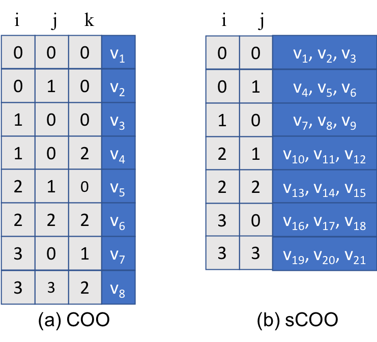
Figure 1. COO format for a general sparse tensor and sCOO format (Li et al., 2016) for a semi-sparse tensor.

3.2. Parallel Implementations based on COO

Table 1 presents the operational intensity of each kernel using a cubical third-order tensor, while all the implementations in the benchmark suite support arbitrary tensor orders. Operational intensity (OI) is the ratio of bytes required per floating point operation for a given computation. For all operations except Mttkrp, we have a pre-processing stage to allocate output tensor space along with their indices.

The implementations of Tew and Ts follow directly from their Equations, (1) and (2), that is one loop over all non-zero values to do the corresponding computation. In the pre-precessing stage, we allocate and set indices for the output tensors due to their easy-to-predict non-zero pattern. Tew and Ts have the smallest operational intensity: $1/12$ and $1/8$. We will use Ttv algorithm as a representative to explain the similar Ttm algorithms as well; Ttm algorithms can be found in (Li et al., 2016; Ma et al., 2018), and Mttkrp algorithms can be easily found in literatures and software (Li et al., 2018c; Bader et al., 2017; Vervliet et al., 2016; Li et al., 2018a).

Table 1. The analysis of kernel algorithms for third-order cubical tensors ($\bm{\mathscr{{X}}}\in\mathbb{R}^{I\times I\times I}$). We consider all input tensors with $M$ non-zero entries and $M_{F}$ fibers, $I\ll M_{\smaller{\mathrm{F}}}\ll M$. The indices use $32$ bits, and values are single-precision floating-point numbers with $32$ bits as well.

Kernels	Work	Memory Access (#Bytes)		OI
	(#Flops)	COO	HiCOO
Tew	$M$	$12M$	$12M$	$1/12$
Ts	$M$	$8M$	$8M$	$1/8$
Ttv	$2M$	$12M+12M_{\smaller{\mathrm{F}}}$	$12M+12M_{\smaller{\mathrm{F}}}$	$\sim 1/6$
Ttm	$2MR$	$4MR+4M_{\smaller{\mathrm{F}}}R$	$4MR+4M_{\smaller{\mathrm{F}}}R$	$\sim 1/2$
		$+8M+8M_{\smaller{\mathrm{F}}}$	$+8M+8M_{\smaller{\mathrm{F}}}$
Mttkrp	$3MR$	$12MR+16M$	$12Rmin\{n_{b}M_{\smaller{\mathrm{B}}},M\}$	$\sim 1/4$
			$+7M+20n_{b}$

^∗ We consider only one-level Cache with the minimum cache size to satisfy the data reuse in algorithms.

3.2.1. Multicore CPU

We use a sparse-dense property for a sparse tensor times a dense vector/matrix (Ttv and Ttm), introduced by Li et al. (Li et al., 2016). That is, if the computation is between a sparse mode of a tensor and a dense vector from the vector itself or a matrix, this mode will become dense in the output; and the other modes keep the same non-zero distribution (or sparsity) with the original modes of the input tensor. This property makes pre-allocating space for the outputs of Ttv and Ttm possible, with the help of the sCOO format for semi-sparse tensors. Introducing this property is good for parallelization by avoiding output data races and dynamic memory allocation, especially useful for GPU implementations.

Algorithm 1 COO-Ttv-OMP algorithm.

1:A third-order sparse tensor $\bm{\mathscr{{X}}}\in\mathbb{R}^{I\times J\times K}$ with $M$ non-zeros in COO format, dense vector $\bm{\mathbf{{V}}}\in\mathbb{R}^{K}$, and an integer $n$ ($=3$);

2:Sparse tensor $\bm{\mathscr{{Y}}}\in\mathbb{R}^{I\times J}$ in COO format;

3:$\triangleright$ $\bm{\mathscr{{Y}}}=\bm{\mathscr{{X}}}\times_{n}\bm{\mathbf{{v}}}$

4:Pre-process to obtain $M_{\smaller{\mathrm{F}}}$, the number of mode-n fibers of $\bm{\mathscr{{X}}}$ and $f_{\smaller{\mathrm{ptr}}}$, the beginning of each $\bm{\mathscr{{X}}}$’s mode-n fiber, size $M_{\smaller{\mathrm{F}}}$.

5:Pre-allocate $\bm{\mathscr{{Y}}}$ space with $M_{\smaller{\mathrm{F}}}$ non-zeros and their indices;

6:

7:parfor $f=1,\dots,M_{\smaller{\mathrm{F}}}$ do

8:    $f_{X}=f_{\smaller{\mathrm{ptr}}}(f)$

9:    $\mathrm{inds}^{1}_{Y}(f)=\mathrm{inds}^{1}_{X}(f_{X})$

10:    $\mathrm{inds}^{2}_{Y}(f)=\mathrm{inds}^{2}_{X}(f_{X})$

11:    $v=\mathrm{val}_{Y}(f)$

12:    for $m=f_{X},\dots,f_{\smaller{\mathrm{ptr}}}(f+1)-1$ do

13:        $k=\mathrm{inds}^{3}_{X}(m)$

14:        $v+=\mathrm{val}_{X}(m)\times u(k)$     

15:

16:Return $\bm{\mathscr{{Y}}}$;

COO-Ttv-OMP is illustrated in Algorithm 1, firstly proposed in this work. We first pre-process the input tensor $\bm{\mathscr{{X}}}$ to record the locations of mode-$n$ fibers. According to the sparse-dense property, the output $\bm{\mathscr{{Y}}}$ is pre-allocated with $M_{\smaller{\mathrm{F}}}$ non-zeros and its indices $i,j$ the same as in $\bm{\mathscr{{X}}}$. The storage is consists of $16M$ for $\bm{\mathscr{{X}}}$, $4I$ for $\bm{\mathbf{{v}}}$, and $12M_{\smaller{\mathrm{F}}}$ for $\bm{\mathscr{{Y}}}$ . The number of floating-point operations (#Flops) is $2M$. The memory access in Table 1 counts $4M$ bytes for $\bm{\mathbf{{v}}}$ because of its irregular and unpredictable memory access introduced by index-$k$. Data reuse of $\bm{\mathbf{{v}}}$ could happen if its access has or gains a good localized pattern naturally or from reordering techniques (Smith et al., 2015; Li et al., 2019b), similarly for the matrices in Ttm and Mttkrp. Thus, their performance could be improved due to reductions in memory pressure. The operational intensity is approximately $1/6$ by ignoring less significant terms. COO-Ttm-OMP is similar to COO-Ttv-OMP with the output as a semi-sparse tensor stored in sCOO format. They are both parallelized for independent fibers, but work imbalance may exist because of different fiber lengths of sparse tensor $\bm{\mathscr{{X}}}$.

COO-Mttkrp is widely used in Tensor Toolbox (Bader et al., 2017), Tensorlab (Vervliet et al., 2016); and COO-Mttkrp-OMP is implemented in ParTI library (Li et al., 2018a). Each row of $\tilde{\bm{\mathbf{{A}}}}$ is updated by scaling the dot product of two rows of matrices $\bm{\mathbf{{B}}}$ and $\bm{\mathbf{{C}}}$ by the non-zero value of $\bm{\mathscr{{X}}}$. Its operational intensity is approximately $1/4$ again by ignoring less expensive terms. COO-Mttkrp-OMP is parallelized by non-zeros, but with atomic operations to protect output matrix. The data race may influence its performance differently depending on non-zero distributions of an input tensor.

3.2.2. GPU

COO-Tew-GPU,-Ts-GPU, and -Ttv-GPU use one-dimensional CUDA grids of one-dimensional thread blocks to parallelize non-zeros and fibers respectively. For example, $M$ non-zeros are assigned to $M/256$ thread blocks with 256 threads for each. Again, due to the potential unbalanced fiber lengths, COO-Ttv-GPU could suffer more performance drop. While COO-Ttm-GPU and -Mttkrp-GPU use one-dimensional grids of two-dimensional thread blocks to parallelize the dense matrices, both of them are implemented in ParTI library (Li et al., 2018a). In COO-Ttm-GPU algorithm, the x-dimension of thread blocks are used to represent matrix columns for GPU memory coalescing, while y-dimension represents non-zeros. (Refer to details in (Ma et al., 2018).) Be aware that the load imbalance still exists for COO-Ttv and COO-Ttm, and also data race for COO-Mttkrp.

3.3. Hierarchical Coordinate (HiCOO)

Hierarchical Coordinate (HiCOO) (Li et al., 2018c) is derived from COO format but further compresses tensor indices in units of sparse blocks with a pre-specified block size $B$. It represents tensor indices using two-level block and element indices, with element indices stored in only $8$-bit. An extra block pointer array $bptr$ is needed to store the starting locations of every fiber. Figure 2(a) shows HiCOO representation for the same tensor in Figure 1(a) in $2\times 2\times 2$ blocks. The same with COO format, HiCOO does not assume any mode order, and only one representation of a sparse tensor is enough for all its computations. While HiCOO saves the tensor storage from two aspects: 1) shorter bit-length for element indices; 2) shortened array length for block indices. Readers can refer to more details in the paper (Li et al., 2018c).

In this work we introduce two variants based on HiCOO format: gHiCOO and sHiCOO. gHiCOO is a generalization of HiCOO format for a general sparse tensor (Figure 2(b)) and sHiCOO is for semi-sparse tensors with dense mode(s) (Figure 2(c)). Concluded by the prior work (Li et al., 2018c), HiCOO could not be beneficial for hyper-sparse tensors where most tensor blocks only consist of one or few non-zeros. To conquer this problem, we propose gHiCOO where we can pick which modes to be compressed in units of blocks for HiCOO and which stay in COO format. Figure 2(b) chooses to compress modes i and j, leaving mode k in the same index array with Figure 1(a). gHiCOO also provide convenience to implement tensor operations where not all modes are needed during computation, such as Ttv and Ttm. sHiCOO is similar to sCOO but in HiCOO format. Figure 2(c) uses sHiCOO to compress the same semi-sparse tensor in Figure 1(b) with dense mode k. Our format variants could be useful in tensor methods and benchmarking for more efficient space and computation.

Figure 2. HiCOO, gHiCOO formats for general sparse tensors and sHiCOO for semi-sparse tensors.

3.4. Parallel Implementations based on HiCOO

HiCOO parallel implementations are all firstly proposed here except Mttkrp on CPUs (Li et al., 2018c). Advanced techniques such as privatization, lock-avoiding parallel strategies, advanced scheduling (Li et al., 2018c) are not adopted as the purpose of this suite is to act as a reference implementation for the community and also to avoid complicated tuning parameters.

3.4.1. Multicore CPU

Since the pre-processing step deals with allocating space and setting indices for the output tensor in HiCOO rather than COO format, the value computation of HiCOO-Tew-OMP and HiCOO-Ts-OMP is the same with COO-Tew-OMP and COO-Ts-OMP respectively.

HiCOO-Ttv-OMP and HiCOO-Ttm-OMP also pre-allocate the output tensors according to the sparse-dense property. We use gHiCOO format to represent the input tensor $\bm{\mathscr{{X}}}$ by leaving the mode doing the product uncompressed. Therefore, Ttv and Ttm can bypass the blocking nature of HiCOO and be performed without data race between blocks. Then the same computation will be implemented for HiCOO-Ttv-OMP and HiCOO-Ttm-OMP as in their COO counterparts, but pre-allocating the output tensors and their indices in HiCOO or sHiCOO format respectively.

Algorithm 2 HiCOO-Mttkrp-OMP algorithm in mode-1 (Li et al., 2018c).

1:A sparse tensor $\bm{\mathscr{{X}}}\in\mathbb{R}^{I\times J\times K}$ with $M$ non-zeros in HiCOO format, dense matrices $\bm{\mathbf{{B}}}\in\mathbb{R}^{J\times R},\bm{\mathbf{{C}}}\in\mathbb{R}^{K\times R}$, block size $B$;

2:Updated dense matrix $\tilde{\bm{\mathbf{{A}}}}\in\mathbb{R}^{I\times R}$;

3:$\triangleright$ $\tilde{\bm{\mathbf{{A}}}}\leftarrow\bm{\mathscr{{X}}}_{(1)}(\bm{\mathbf{{C}}}\odot\bm{\mathbf{{B}}})$

4:parfor $b=1,\dots,n_{b}$ do

5:    $bi=\mathrm{binds}^{1}(b)$, $bj=\mathrm{binds}^{2}(b)$, $bk=\mathrm{binds}^{3}(b)$;

6:    $\bm{\mathbf{{A}}}_{b}=\bm{\mathbf{{A}}}+bi\cdot B\cdot R$; $\bm{\mathbf{{B}}}_{b}=\bm{\mathbf{{B}}}+bj\cdot B\cdot R$; $\bm{\mathbf{{C}}}_{b}=\bm{\mathbf{{C}}}+bk\cdot B\cdot R$;

7:    for $x=bptr(b),\dots,bptr(b+1)-1$ do $\triangleright$ entry $x$

8:        $ei=\mathrm{einds}^{1}(x)$, $ej=\mathrm{einds}^{2}(x)$, $ek=\mathrm{einds}^{3}(x)$

9:        $value=\mathrm{val}(x)$

10:        for $r=1,\dots,R$ do

11:           $\tilde{A}_{b}(ei,r)+=value\cdot C_{b}(ek,r)\cdot B_{b}(ej,r)$             

12:

13:Return $\tilde{\bm{\mathbf{{A}}}}$;

HiCOO-Mttkrp-OMP is more complicated because indices of all tensor modes are used in this computation, different from Ttv and Ttm where the indices from only one mode are needed. We first block matrices $\bm{\mathbf{{A}}}$, $\bm{\mathbf{{B}}}$, and $\bm{\mathbf{{C}}}$ as $\bm{\mathbf{{A}}}_{b}$, $\bm{\mathbf{{B}}}_{b}$, and $\bm{\mathbf{{C}}}_{b}$ to be reused for the non-zeros inside a tensor block. For each block, we update the values of a block of output matrix $\tilde{\bm{\mathbf{{A}}}}$ using corresponding blocks $\bm{\mathbf{{B}}}_{b}$, and $\bm{\mathbf{{C}}}_{b}$. In this way, we do not need to compute the actual indices $i,j,k$ out, and data locality is increased due to blocking and Morton order sorting when constructing a HiCOO representation (Li et al., 2018c). Different from COO-Mttkrp-OMP, HiCOO-Mttkrp-OMP parallelize tensor blocks rather than all non-zeros.

The analysis of HiCOO algorithms are also listed in Table 1. Since HiCOO-Tew, -Ts, -Ttv, -Ttm all have the same value computation step with COO counterparts, so they have the same behavior except for the storage space, where HiCOO is usually beneficial. However, from our experiments, we still observe some benefits of HiCOO affected by the pre-processing stage. However, HiCOO-Mttkrp has smaller memory access than COO-Mttkrp due to its blocked feature.

3.4.2. GPU

HiCOO-GPU implementations are also the same with COO ones except HiCOO-Mttkrp-GPU. This unoptimized HiCOO-Mttkrp-GPU maps one tensor block to a CUDA thread block, thus the balanced workload by non-zero distribution for COO-Mttkrp disappears, while the atomic operation stays. Therefore, the work imbalance due to different numbers of non-zeros in tensor blocks could be make its performance even worse than COO-Mttkrp-GPU.

4. Tensor Dataset

Table 2. Description of sparse tensors.

No.	Tensors	Order	Dimensions	#Nnzs	Density
r1	vast	3	$165K\times 11K\times 2$	26M	$6.9\times 10^{-3}$
r2	nell2	3	$12K\times 9K\times 29K$	77M	$2.4\times 10^{-5}$
r3	choa	3	$712K\times 10K\times 767$	27M	$5.0\times 10^{-6}$
r4	darpa	3	$22K\times 22K\times 24M$	28M	$2.4\times 10^{-9}$
r5	fb-m	3	$23M\times 23M\times 166$	100M	$1.1\times 10^{-9}$
r6	fb-s	3	$39M\times 39M\times 532$	140M	$1.7\times 10^{-10}$
r7	flickr	3	$320K\times 28M\times 1.6M$	113M	$7.8\times 10^{-12}$
r8	deli	3	$533K\times 17M\times 2.5M$	140M	$6.1\times 10^{-12}$
r9	nell1	3	$2.9M\times 2.1M\times 25M$	144M	$9.1\times 10^{-13}$
r10	crime4d	4	$6K\times 24\times 77\times 32$	5M	$1.5\times 10^{-2}$
r11	uber4d	4	$183\times 24\times 1140\times 1717$	3M	$3.9\times 10^{-4}$
r12	nips4d	4	$2K\times 3K\times 14K\times 17$	3M	$1.8\times 10^{-6}$
r13	enron4d	4	$6K\times 6K\times 244K\times 1K$	54M	$5.5\times 10^{-9}$
r14	flickr4d	4	$320K\times 28M\times 1.6M\times 731$	113M	$1.1\times 10^{-14}$
r15	deli4d	4	$533K\times 17M\times 2.5M\times 1K$	140M	$4.3\times 10^{-15}$

This benchmark suite uses sparse tensors derived from real-world applications from online collections (Smith et al., 2017; Jeon et al., 2015b; Perros et al., 2017). It also generates synthetic sparse tensors based on graph models that preserve the properties of real-world graphs. The benchmark suite can be run against any set of tensors provided that they are expressed using coordinate format.

4.1. Tensors From Real World Applications

The tensors taken from real-world applications are described in Table 2 sorted by tensor order and decreasing density. They are taken from The Formidable Repository of Open Sparse Tensors and Tools (FROSTT) dataset (Smith et al., 2017), the HaTen2 (Jeon et al., 2015a) dataset, and one built from electronic medical records from Children’s Healthcare of Atlanta (Perros et al., 2017). These tensors were chosen to represent a wide range of domains: pattern recognition (vast, nips4d), natural language processing (nell2, nell1), healthcare analytics (choa), recommendation systems (deli, deli4d, flickr4d), crime detection (crime4d), anomaly detection (enron4d).

4.2. Synthetic Tensor Generation

The Kronecker graph model (Leskovec et al., 2010) and the biased power law generator from the FireHose streaming benchmark (Anderson and Plimpton, 2015) were extended to generate 3- and 4-dimensional tensors. These methods were selected because the resultant graphs follow the power law distribution, exhibit a small diameter, and have a high average clustering coefficient.

The software to generate synthetic tensors is included in the benchmark suite and the synthetic tensors used in our experiments are described in Table 3 in a period order of ”small, medium, large”. The regular 3D and 4D tensors, which are equidimensional along each mode, are generated using the Kronecker generator. The irregular 3D and 4D tensors are generated using the biased power law streaming generator. The 3D irregular tensors have one mode completely dense and much smaller compared to the two other modes which are equidimensional and sparse. Two modes of the irregular 4D tensors are hypersparse and equidimensional, and the other two dimensions are entirely dense and smaller.

4.2.1. The Stochastic Kronecker Graph Model

The Stochastic Kronecker graph model (Leskovec et al., 2010) is a fractal growth model that preserves the previously listed properties of real-world graphs. We extended this approach to generate sparse tensors of order $N$ by accepting the initiator as a tensor $\tau_{1}$ with $N$ modes. Similar to the Stochastic Kronecker graph model, by taking the repeated Kronecker product of $\tau_{1}$ for $n$ times, a larger $N$th-order tensor $\tau_{n}$ is produced. With Bernoulli sampling, $\tau_{n}$ can be realized as a large sparse tensor representing the resultant hyper-graph that follow the properties of real-world networks.

The exponential growth of Kronecker multiplication limits the sizes of $N$th-order tensors that can be generated. We overcome this by performing an additional iteration of Kronecker multiplication and strip off the tensor coordinates that fall outside the given size along each mode.

4.2.2. The Power Law Generator

The power law generated graphs do not possess a high average clustering coefficient, there is no restriction on the size of the graph generated. The generator produces a stream of edges that when combined form a graph respecting the power law distribution. This is used to create tensors by combining together the sparse graphs to form slices of a third order tensor which is hypergraph. This process, when repeated on 3rd order tensors can generate a sparse tensor with $N$ modes.

Table 3. Description of synthetic tensors generated (Gen.) with Kronecker and Power law generators indicated as Kron. and PL respectively.

No.	Tensors	Gen.	Order	Dimensions	#Nnzs	Density
s1	regS	Kron.	3	$(65K)^{3}$	1.1M	$3.72\times 10^{-9}$
s2	regM	Kron.	3	$(1.1M)^{3}$	11.5M	$9.97\times 10^{-12}$
s3	regL	Kron.	3	$(8.3M)^{3}$	94M	$1.61\times 10^{-13}$
s4	irrS	PL	3	$(32K)^{2}\times 76$	1M	$1.26\times 10^{-5}$
s5	irrM	PL	3	$(524K)^{2}\times 126$	10M	$1.43\times 10^{-6}$
s6	irrL	PL	3	$(4.2M)^{2}\times 168$	84M	$2.86\times 10^{-8}$
s7	regS4d	Kron.	4	$(8.2K)^{4}$	1M	$2.26\times 10^{-10}$
s8	regM4d	Kron.	4	$(2.1M)^{4}$	11.2M	$5.83\times 10^{-19}$
s9	regL4d	Kron.	4	$(8.3M)^{4}$	110M	$2.23\times 10^{-20}$
s10	irrS4d	PL	4	$(1.6M)^{3}\times 82$	1.0M	$2.90\times 10^{-9}$
s11	irrM4d	PL	4	$(2.6M)^{3}\times 144$	10.8M	$4.17\times 10^{-12}$
s12	irrL4d	PL	4	$(4.2M)^{3}\times 226$	100M	$6.0\times 10^{-15}$
s13	irr2S4d	PL	4	$(1.0M)^{2}\times 122\times 436$	1.6M	$2.81\times 10^{-11}$
s14	irr2M4d	PL	4	$(4.2M)^{2}\times 232\times 746$	19.9M	$6.53\times 10^{-12}$
s15	irr2L4d	PL	4	$(8.3M)^{2}\times 952\times 324$	109M	$5.1\times 10^{-12}$

5. Experimental Results

We test our tensor kernels on four parallel platforms including Intel CPUs and NVIDIA GPUs and build Roofline performance models to measure our performance bounds for detailed analysis.

5.1. Configurations

5.1.1. Platforms

We run the experiments on four parallel platforms, the parameters of which are listed in Table 4. All Intel platforms are non-uniform memory access (NUMA) machines with 2-4 NUMA nodes. We calculate the peak single-precision (SP) floating point performance and main/global-memory bandwidth from these parameters. The peak SP performance of all machines is above 1 TFLOPS. GPUs show advantages in peak performance and memory bandwidth over CPUs by approximately $4-12\times$ and $3-7\times$ respectively.

Table 4. Platform parameters.

Parameters	Intel CPUs		NVIDIA GPUs
	Bluesky	Wingtip	DGX-1P	DGX-1V
Processor	Intel Xeon	Intel Xeon	NVIDIA	NVIDIA
	Gold 6126	E7-4850v3	Tesla P100	Tesla V100
Microarch	Skylake	Haswell	Pascal	Volta
Frequency	2.60 GHz	2.20 GHz	1.48 GHz	1.53 GHz
#Cores	24 ($12\times 2$)	56 ($14\times 4$)	3584	5120
Peak SP	1.0	2.0	10.6	14.9
Perf.	TFLOPS	TFLOPS	TFLOPS	TFLOPS
LLC size	19 MB	35 MB	3 MB	6 MB
Mem. size	196 GB	2114 GB	16 GB	16 GB
Mem. type	DDR4	DDR4	HBM2	HBM2
Mem. freq.	2.666 GHz	2.133 GHz	0.715 GHz	0.877 GHz
Mem. BW	256 GB/s	273 GB/s	732 GB/s	900 GB/s
Compiler	gcc 7.1.0	gcc 5.5.0	CUDA Tkit 9.1	CUDA Tkit 9.0

5.1.2. Kernel Implementation Details

Since our data is naturally sorted in a particular mode order, COO implementations could take some advantages from the better data locality. The addition operation is the representative of Tew and the multiplication operation represents Ts; the performance using different operations are quite similar in our experiments. For multicore CPU implementations, we use OpenMP for parallelization with different scheduling strategies, with the number of threads is set to the number of physical cores. “omp atomic” is used to deal with data race in Mttkrp, and “omp simd” is for vectorization of Ttm and Mttkrp. We use “numactl –interleave=all –physcpubind” to interleave memory allocation for better memory bandwidth usage and thread binding for lower scheduling overhead. For GPU implementations, “atomicAdd” is used in Mttkrp. For HiCOO format, we fix the block size to $128$ to fit into the last-level cache in all platforms and use only 8 bits to store element indices. We use $16$ as the column size for matrices in Ttm and Mttkrp, to reflect the low-rank feature in popular tensor methods. We run all kernels five times to get the average; the time of Ttv, Ttm, and Mttkrp is further averaged among all tensor modes.

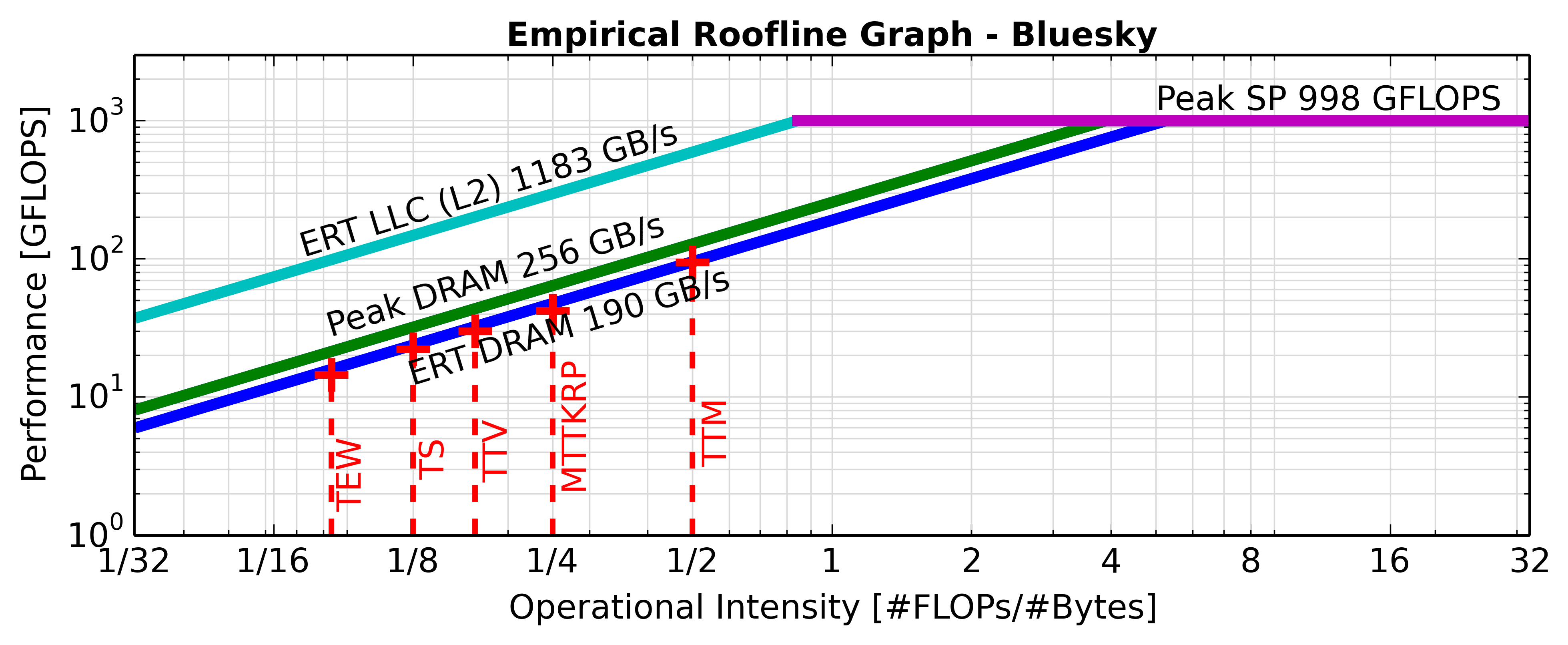
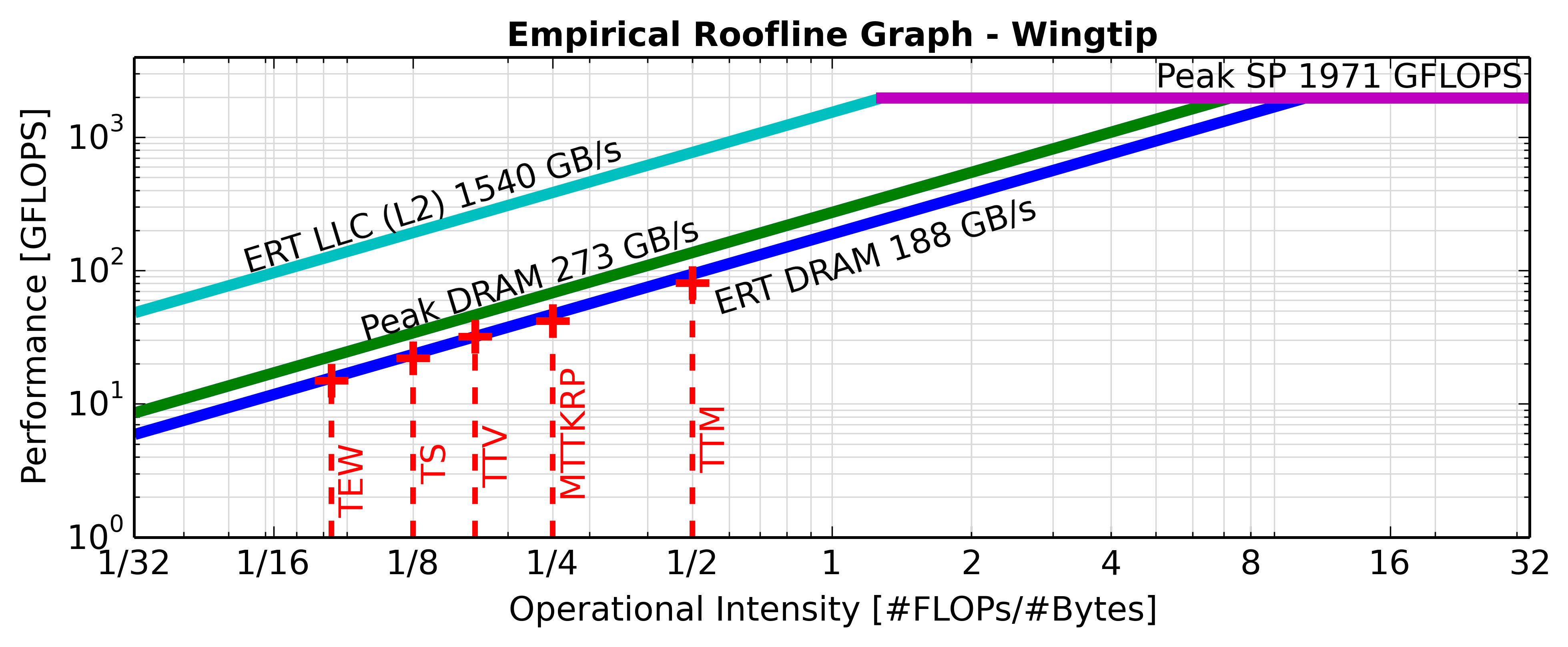
(a) Bluesky	(b) Wingtip
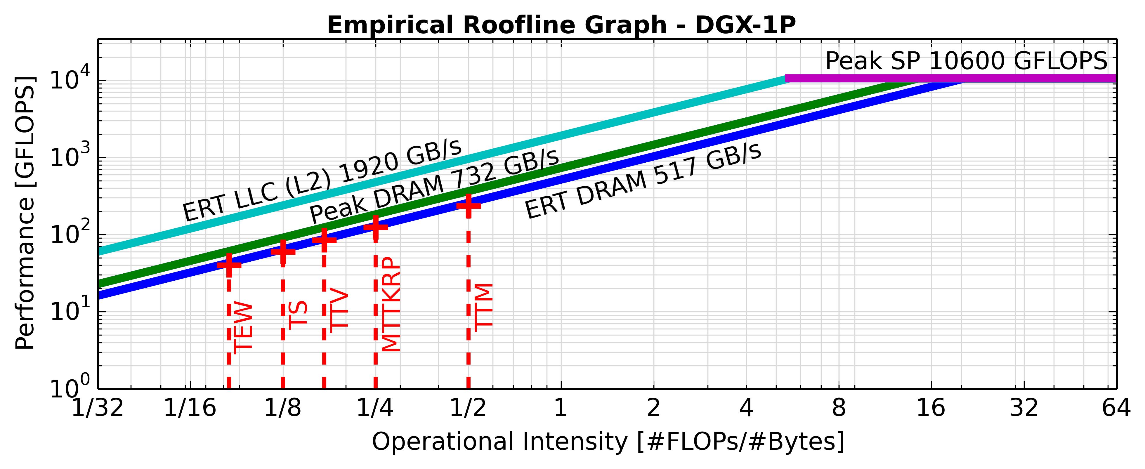
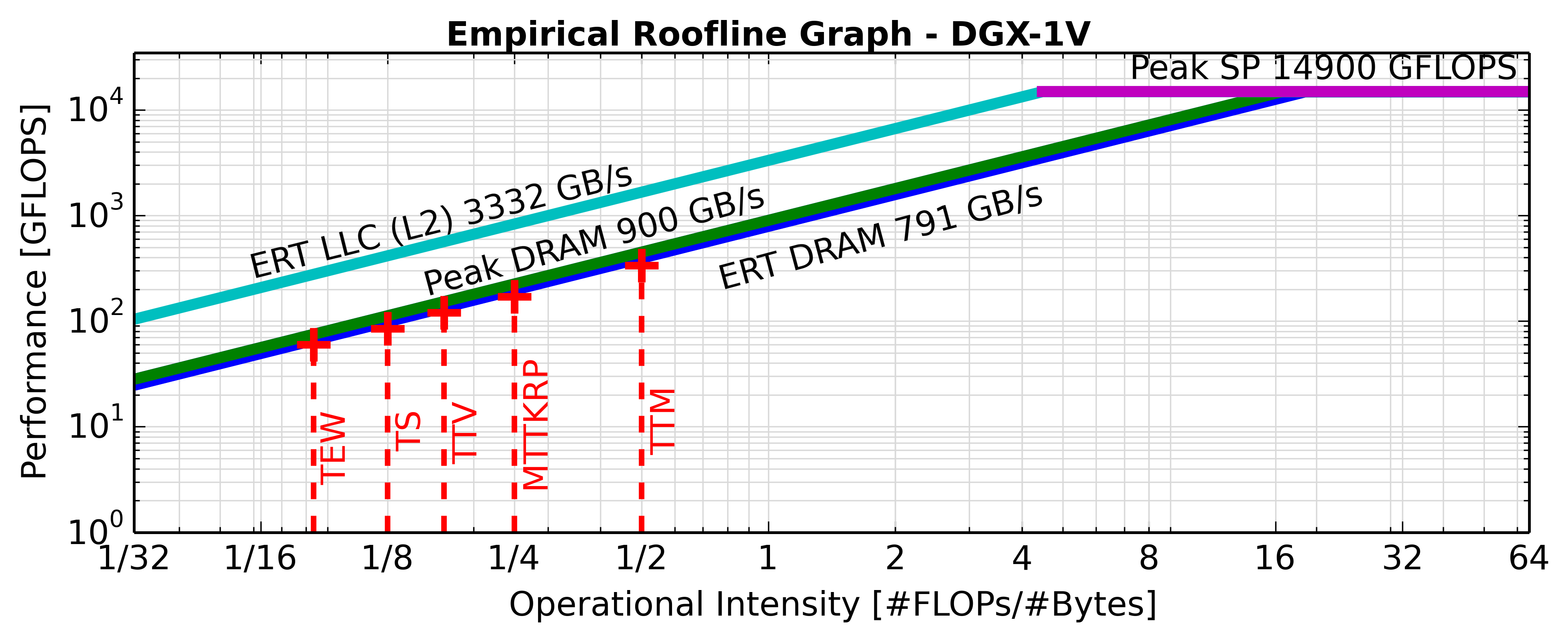
(c) DGX-1P	(d) DGX-1V

Figure 3. Roofline models marked with the operational intensities of tensor kernels.

5.2. Roofline Performance Models

The Roofline performance model (Williams et al., 2009; Williams, 2008) is a graphical representation of machine characteristics. It is employed for performance analysis in various application domains: digital signal processing, e.g., Spiral  (Ofenbeck et al., 2014), sparse/dense linear algebra (Williams, 2008; Zhang et al., 2017), and Lattice Boltzmann Magnetohydrodynamics (LBMHD) (Williams, 2008). The Empirical Roofline Tool (ERT) (Lo et al., 2015), included into Intel Advisor tool, automates measuring the target machine characteristics. ERT automatically generates Roofline data including the maximum bandwidth for various levels of the memory hierarchy which are obtained by testing a variety of micro-kernels . ERT can utilize MPI, OpenMP, and CUDA for parallelization; we configure it to the corresponding compiler in Table 4 for tests.

Figure 3 plots the Roofline models for the four platforms in Table 4 with DRAM and last-level cache (LLC) bandwidth tested from ERT, and the theoretical peak SP performance and DRAM bandwidth (not cache-aware) for reference. We mark the operational intensities (#Flops/#Bytes) of our tensor kernels calculated from Table 1 overlying with Roofline models. “ERT-DRAM” bandwidth is the obtainable bandwidth from benchmarking micro-kernels, thus OIs of all the tensor kernels are marked on this line. From this figure, all of the sparse tensor kernels we consider are main or global memory bound for CPUs and GPUs respectively. Higher bandwidth will accelerate kernel execution, while other factors such as better data reuse (cache utilization) lowering memory access pressure will also lead to performance improvement. We use the computed obtainable performance of all tensor kernels as the upper bounds in our performance figures below (called “Roofline performance”), calculated by timing an OI value with the “ERT-DRAM” bandwidth. The OI value is an accurate #Flops/#Bytes ratio by taking different tensor features into account, especially for Ttv and Ttm because of the $M_{\smaller{\mathrm{F}}}$ term in Table 1.

(a) Real tensors

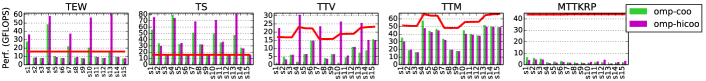
(b) Synthetic tensors

Figure 4. Single-precision performance of tensor kernels on the Bluesky platform with the Roofline performance.

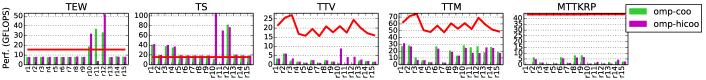
(a) Real tensors

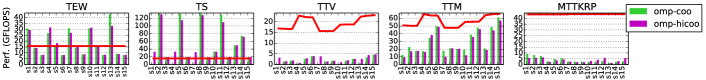
(b) Synthetic tensors

Figure 5. Single-precision performance of tensor kernels on the Wingtip platform with the Roofline performance.

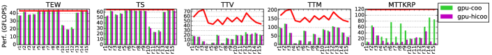
(a) Real tensors

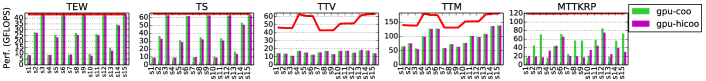
(b) Synthetic tensors

Figure 6. Single-precision performance of tensor kernels on NVIDIA DGX-1P with the Roofline performance.

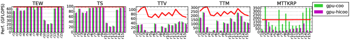
(a) Real tensors

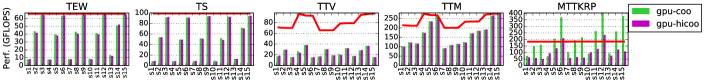
(b) Synthetic tensors

Figure 7. Single-precision performance of tensor kernels on NVIDIA DGX-1V with the Roofline performance.

5.3. Performance

This section presents the performance of all the five tensor kernels on two datasets, real and synthetic, for four platforms. The performance in GFLOPS of each tensor kernel is calculated from #Flops (in Table 1) divided by the measured execution time. X-axis represents tensors using the numbers in Tables 2 and 3 from different datasets.

Observation 1: Achieved performance is diverse and hard to predict, which varies with the dimension sizes and non-zero patterns of tensors, platforms, and data formats.

From Figures 4, 5, 6 and 7, the actual performance in GFLOPS are extremely diverse between tensor kernels, data formats, platforms, and datasets. Take synthetic dataset as an example, the achieved performance varies from 0.8 GFLOPS (regS in COO) to 81 GLOPS (irr2S4d in HiCOO) in Figure 4 on Bluesky platform. Besides, the average performance of the five kernels ranges a lot as well. Tew, Ts, Ttv, Ttm, Mttkrp kernels achieve an average of $14.6$, $35.1$, $6.3$, $37.7$, and $2.7$ GFLOPS respectively for COO format, and $22.3$, $40.8$, $14.4$, $35.8$, and $2.6$ GFLOPS respectively for HiCOO format. This also shows HiCOO on average behaves better than COO format for Tew, Ts, and Ttv and gets similar performance on Ttm and Mttkrp. Even for the performance efficiency (or bandwidth efficiency), these kernels still vary a large range from the lowest 2% (Mttkrp on irr2S4d) to 353% (Ts on regS) for COO format and 2% (Mttkrp on irr2S4d) - 479% (Ts on regS). (The above 100% efficiency phenomenon will be explained below.) Also, quite different performance numbers are observed between real and synthetic datasets under the same tensor kernel. For Wingtip platform in Figure 5, Ttv shows much lower GFLOPS numbers than those on Bluesky. Though we observe some trend especially for synthetic dataset and Ttm operation, generally it is hard to predict the performance of a sparse kernel, even operating with a dense matrix or vector.

Observation 2: Performance is generally below the Roofline performance calculated from main/global memory bandwidth except for some small tensors fitting into caches or algorithms with good data locality thus making a good use of caches.

Most of cases in Figures 4, 5, 6 and 7 fall below the red Roofline performance line calculated from main/global memory bandwidth from Figure 3 except for some case of Tew and Ts on Bluesky and Wingtip CPU platforms and Mttkrp on DGX-1V GPU platform. Take Figure 4 as an example again, the tensors exceed Roofline performance are all small tensors with around 1M non-zeros: regS, irrS, regS4d, irrS4d, and irr2S4d for Tew, all small and medium synthetic tensors and small real tensors with 3-5M non-zeros: crime4d, uber4d, and nips4d. The last level cache size of Bluesky is 19 MB which could reside three tensor values each with around 1.6M non-zeros of Tew and two tensor values each with around 2.4M non-zeros of Ts. These numbers matches with the small synthetic and real tensors, while the medium tensors also gain some cache benefit. For Mttkrp on DGX-1V, COO-Mttkrp-GPU gets higher performance than Roofline more on irregular-shaped tensors in synthetic dataset. And the tensors achieve high performance on DGX-1P are easier to get break the upper bound on DGX-1V. One reason is that V100 GPU architecture has a twice larger LLC (6M) than P100; besides, V100 get improved atomic operation performance which could benefit Mttkrp; another reason is that they may have very good data reuse or small working-set size, e.g., tensors with a very short mode, so it is cache that offers the data injection rate rather than off-chip memory; lastly, the integer and floating-point operations have independent data-paths for instruction issuing on Volta architecture. Therefore, address computation which is extensively used in Mttkrp can be overlapped with floating-point operations, which may mitigate the waiting time for address calculation compared with earlier GPU architectures.

Observation 3: It is hard to obtain good performance efficiency for non-streaming kernels on multi-socket CPU machines because of NUMA effect, which could be even harder than on GPUs.

On Bluesky (Figure 4), the average performance efficiency of Ttv, Ttm, and Mttkrp is 31%, 64%, 6% for COO format, and 73%, 61%, 5% for HiCOO format; while the numbers are 9%, 52%, 9% for COO and 13%, 47%, 9% for HiCOO on Wingtip (Figure 5). Though Mttkrp behaves a little higher efficiency on Wingtip, its efficiency is still very low. The increment could come from better parallelism of Wingtip with 56 cores. On DGX-1P GPU (Figure 6), the average performance efficiency of Ttv, Ttm, and Mttkrp is 30%, 60%, 40% for COO format, and 30%, 60%, 28% for HiCOO format; while the numbers are 30%, 69%, 110% for COO and 30%, 69%, 57% for HiCOO on DGX-1V (Figure 7). The efficiency numbers on four-socket Wingtip CPU are all lower than those on DGX-1P and DGX-1V GPUs, while Ttv and Ttm achieves better or similar efficiency than the two GPUs on two-socket Bluesky CPU.

Observation 4: HiCOO algorithms is faster than or similar to COO counterparts because of its better local locality and smaller memory footprint, except Mttkrp on GPUs where load imbalance and lower parallelism play more important roles.

From the average efficiency and performance numbers shown in Observation 1 and 3, HiCOO on average behaves better than COO format for Tew, Ts, and Ttv and gets similar performance on Ttm and Mttkrp on CPU platforms. On the two GPUs, due to their smaller last-level cache size, HiCOO does not benefit as much as on CPUs. From Figures 6 and 7, HiCOO gets very similar performance on Tew, Ts, Ttv, and Ttm because of their similar execution code for tensor value computation. While HiCOO-Mttkrp behaves worse than COO-Mttkrp because of their different parallel strategies. HiCOO parallelize tensor blocks with severe load imbalance issue and lower parallelism compared to COO-Mttkrp algorithm. Thus, to better use HiCOO format, a careful tuning need to be done according to architecture features.

Observation 5: Different datasets expose very different performance behavior, which shows the importance of synthetic datasets to performance benchmarking and analysis.

Compare the performance trend of real and synthetic datasets. Tew and Ts show obvious period trend from high to low or low to high on CPUs and GPUs respectively due to different cache sizes on synthetic dataset, while it is hard to find trends in real dataset. Ttv and especially Ttm show a matching trend with the Roofline predicted performance for both real and synthetic tensors. Since real tensors are from diverse real application scenarios, it is hard to do benchmarking and performance analysis solely based on them. Besides, real tensors are limited due to data privacy and other publicity issues. Extracting features from real tensors as a basis to create more complete synthetic tensors would be very helpful for sparse tensor research.

Overall, diverse performance behavior is observed among the five kernels and between the COO and HiCOO formats on the Intel CPU and NVIDIA GPU platforms. Our benchmark performance is still lower than the theoretical Roofline for most cases, especially for Mttkrp. Advanced performance optimization could be further explored, such as the lock-avoiding techniques employed in (Li et al., 2018c).

6. Related Work

Work related to this benchmark suite includes various benchmarking collections and synthetic benchmark data generation. This benchmark suite is distinct from previous efforts in its focus on multi-dimensional tensors combined with both real and synthetic input.

Benchmark suites measure machine attributes and exemplify computing patterns. Benchmarks that measure specific machine attributes include LINPACK (Dongarra et al., 2003), SPEC (Dixit, 1991), STREAM (McCalpin, 2007), GeekBench (GeekBench, 4), Multimaps (Snavely et al., 2002), Bandwidth (Smith, 2008), and others. Most of them aim to measure memory bandwidth achieved under varying conditions and a few target architecture floating-point capabilities. Benchmark suites are often organized around the concept of application exemplars. These suites emulate common patterns and behaviors in application classes of interest. Several examples of these suites have been published: LAPACK/ScaLAPACK for dense linear algebra (Blackford et al., 1996), Colella’s Seven Motif’s (Colella, 2004) for scientific computing, PARSEC (Bienia et al., 2008) and SPLASH2 (Woo et al., 1995), Rodinia (Che et al., 2009), Graph500 (Murphy et al., 2010), SparseBench (Dongarra et al., 2001), GAP (Beamer et al., 2015), SSCA#2 (Kepner et al., 2005), and Tartan (Li et al., 2018b) are just a few.

Several approaches to synthetic graph generation have been proposed. Our work extends two of these, power law graphs from Firehose, and Kronecker graphs from Graph500 (Murphy et al., 2010). FireHose is a suite of stream processing benchmarks (Anderson and Plimpton, 2015), one of a front-end generator of which is the biased power law generator. Existing synthetic tensor generators like SimTensor (Fanaee-T and Gama, 2016), Nway Toolbox (Andersson and Bro, 2000), and the Tensor Toolbox (Bader et al., 2017) are specific to tensors with Tucker (Tucker, 1966), CANDECOMP/PARAFAC decomposition (Carroll and Chang, 1970; Carroll et al., 1980) structures or particular data distributions. This paper provides a starting point to generate sparse tensors that preserve the properties of real-world or multi-attributed graphs that can be realized as higher-order sparse tensors.

Many libraries support sparse tensor methods, such as Tensor Toolbox (Bader et al., 2017), Nway Toolbox (Andersson and Bro, 2000), Tensorlab (Vervliet et al., 2016), TACO (Kjolstad et al., 2017), SPLATT (Smith et al., 2015), and ParTI (Li et al., 2018a). As a benchmark suite, we supply widely-adopted reference implementations and make continuously effort to include state-of-the-art algorithms and data structures as well.

7. Conclusion

This paper presents a benchmark suite targeting sparse tensor kernels. Operations on sparse tensors are common in a wide range of important applications. The operations are memory bound and often dominate application performance. This benchmark suite identifies important kernels and data representations and provides reference implementations to aid the community in effectively sharing and comparing performance and optimization results. Two methods for synthetic tensor generation are provided by preserving the properties of real-world graphs. A subset of possible synthetic tensors are used in this paper. The tool provides the ability to generate custom synthetic tensors in a reproducible manner.

Five observations are made based on performance analysis over Roofline models to gain insights of sparse tensor behavior across architectures. This benchmark suite is a continuous effort: additional operations, such as TTM-chain in Tucker decomposition, tensor contraction, a sparse tensor with a sparse vector/matrix operations; more complete tensor methods, such as CANDECOMP/PARAFAC and Tucker decompositions; data representations, such as compressed sparse fiber (CSF) (Smith et al., 2015), balanced CSF (BCSF) (Israt Nisa, 2019); more platforms, such as distributed systems, multiple GPUs, and other new architectures (e.g., FPGAs and Emu (Dysart et al., 2016; Hein et al., 2018)) will be included to the suite in the future.

References

- (1)
- Anandkumar et al. (2014) Animashree Anandkumar, Rong Ge, Daniel Hsu, Sham M. Kakade, and Matus Telgarsky. 2014. Tensor Decompositions for Learning Latent Variable Models. J. Mach. Learn. Res. 15, 1 (Jan. 2014), 2773–2832.
- Anderson and Plimpton (2015) Karl Anderson and Steve Plimpton. 2015. FireHose Streaming Benchmarks. Technical Report. Sandia National Laboratory.
- Andersson and Bro (2000) Claus A Andersson and Rasmus Bro. 2000. The N-way Toolbox for MATLAB. Chemometrics and Intelligent Laboratory Systems 52, 1 (Aug 2000), 1–4.
- Bader et al. (2017) Brett W. Bader, Tamara G. Kolda, et al. 2017. MATLAB Tensor Toolbox (Version 3.0-dev). Available online. https://www.tensortoolbox.org
- Baskaran et al. (2012) M. Baskaran, B. Meister, N. Vasilache, and R. Lethin. 2012. Efficient and scalable computations with sparse tensors. In High Performance Extreme Computing (HPEC), 2012 IEEE Conference on. 1–6. https://doi.org/10.1109/HPEC.2012.6408676
- Beamer et al. (2015) Scott Beamer, Krste Asanović, and David Patterson. 2015. The GAP benchmark suite. arXiv preprint arXiv:1508.03619 (2015).
- Bienia et al. (2008) Christian Bienia, Sanjeev Kumar, Jaswinder Pal Singh, and Kai Li. 2008. The PARSEC benchmark suite: Characterization and architectural implications. In Proceedings of the 17th international conference on Parallel architectures and compilation techniques. ACM, 72–81.
- Blackford et al. (1996) Laura Susan Blackford, J. Choi, A. Cleary, A. Petitet, R. C. Whaley, J. Demmel, I. Dhillon, K. Stanley, J. Dongarra, S. Hammarling, G. Henry, and D. Walker. 1996. ScaLAPACK: A Portable Linear Algebra Library for Distributed Memory Computers - Design Issues and Performance. In Proceedings of the 1996 ACM/IEEE Conference on Supercomputing (Supercomputing ’96). IEEE Computer Society, Washington, DC, USA, Article 5. https://doi.org/10.1145/369028.369038
- Carroll and Chang (1970) J. Douglas Carroll and Jih-Jie Chang. 1970. Analysis of individual differences in multidimensional scaling via an n-way generalization of “Eckart-Young” decomposition. Psychometrika 35, 3 (01 Sep 1970), 283–319. https://doi.org/10.1007/BF02310791
- Carroll et al. (1980) J. D. Carroll, S. Pruzansky, and J. B. Kruskal. 1980. CANDELINC: A general approach to multidimensional analysis of many-way arrays with linear constraints on parameters. Psychometrika 45 (1980), 3–24.
- Che et al. (2009) S. Che, M. Boyer, J. Meng, D. Tarjan, J. W. Sheaffer, S. Lee, and K. Skadron. 2009. Rodinia: A benchmark suite for heterogeneous computing. In 2009 IEEE International Symposium on Workload Characterization (IISWC). 44–54. https://doi.org/10.1109/IISWC.2009.5306797
- Chou et al. (2018) Stephen Chou, Fredrik Kjolstad, and Saman Amarasinghe. 2018. Format Abstraction for Sparse Tensor Algebra Compilers. Proc. ACM Program. Lang. 2, OOPSLA, Article 123 (Oct. 2018), 30 pages. https://doi.org/10.1145/3276493
- Cichocki (2014) Andrzej Cichocki. 2014. Era of Big Data Processing: A New Approach via Tensor Networks and Tensor Decompositions. CoRR abs/1403.2048 (2014).
- Cichocki et al. (2016) A. Cichocki, N. Lee, I. V. Oseledets, A. Phan, Q. Zhao, and D. Mandic. 2016. Low-Rank Tensor Networks for Dimensionality Reduction and Large-Scale Optimization Problems: Perspectives and Challenges PART 1. ArXiv e-prints (Sept. 2016). arXiv:cs.NA/1609.00893
- Colella (2004) Phil Colella. 2004. Defining Software Requirements for Scientific Computing. (01 2004).
- De Lathauwer et al. (2017) Lieven De Lathauwer, Nico Vervliet, Martijn Boussé, and Otto Debals. 2017. Dealing with curse and blessing of dimensionality through tensor decompositions.
- Di Napoli et al. (2014) Edoardo Di Napoli, Diego Fabregat-Traver, Gregorio Quintana-Ortí, and Paolo Bientinesi. 2014. Towards an efficient use of the BLAS library for multilinear tensor contractions. Appl. Math. Comput. 235 (2014), 454 – 468. https://doi.org/10.1016/j.amc.2014.02.051
- Dixit (1991) Kaivalya M Dixit. 1991. The SPEC benchmarks. Parallel computing 17, 10-11 (1991), 1195–1209.
- Dongarra et al. (2001) Jack Dongarra, Victor Eijkhout, and Henk van der Vorst. 2001. SparseBench: A sparse iterative benchmark.
- Dongarra et al. (2003) Jack J Dongarra, Piotr Luszczek, and Antoine Petitet. 2003. The LINPACK benchmark: past, present and future. Concurrency and Computation: practice and experience 15, 9 (2003), 803–820.
- Dysart et al. (2016) Timothy Dysart, Peter Kogge, Martin Deneroff, Eric Bovell, Preston Briggs, Jay Brockman, Kenneth Jacobsen, Yujen Juan, Shannon Kuntz, Richard Lethin, Janice McMahon, Chandra Pawar, Martin Perrigo, Sarah Rucker, John Ruttenberg, Max Ruttenberg, and Steve Stein. 2016. Highly Scalable Near Memory Processing with Migrating Threads on the Emu System Architecture. In Proceedings of the Sixth Workshop on Irregular Applications: Architectures and Algorithms (IA3̂ ’16). IEEE Press, Piscataway, NJ, USA, 2–9. https://doi.org/10.1109/IA3.2016.7
- Fanaee-T and Gama (2016) Hadi Fanaee-T and Joao Gama. 2016. SimTensor: A synthetic tensor data generator. arXiv preprint arXiv:1612.03772 (2016).
- GeekBench (4) GeekBench. 4. Primate Labs. http://http://www.geekbench.com/
- Hein et al. (2018) Eric Hein, Tom Conte, Jeffrey S. Young, Srinivas Eswar, Jiajia Li, Patrick Lavin, Richard Vuduc, and Jason Riedy. 2018. An Initial Characterization of the Emu Chick. 2018 IEEE International Parallel and Distributed Processing Symposium Workshops (May 2018), 10.
- Israt Nisa (2019) Aravind Sukumaran-Rajam Richard Vuduc P. Sadayappan Israt Nisa, Jiajia Li. 2019. Load-balanced sparse MTTKRP on GPUs. (To be appeared).
- Jeon et al. (2015b) Inah Jeon, Evangelos E. Papalexakis, U Kang, and Christos Faloutsos. 2015b. HaTen2: Billion-scale Tensor Decompositions. In IEEE International Conference on Data Engineering (ICDE).
- Jeon et al. (2015a) Inah Jeon, Evangelos E. Papalexakis, and Christos Faloutsos U Kang. 2015a. HaTen2: Billion-scale Tensor Decompositions (Version 1.0). Available from http://datalab.snu.ac.kr/haten2/.
- Ji et al. (2012) Shuiwang Ji, Wei Xu, Ming Yang, and Kai Yu. 2012. 3D convolutional neural networks for human action recognition. IEEE transactions on pattern analysis and machine intelligence 35, 1 (2012), 221–231.
- Kaya and Uçar (2018) O. Kaya and B. Uçar. 2018. Parallel Candecomp/Parafac Decomposition of Sparse Tensors Using Dimension Trees. SIAM Journal on Scientific Computing 40, 1 (2018), C99–C130. https://doi.org/10.1137/16M1102744 arXiv:https://doi.org/10.1137/16M1102744
- Kepner et al. (2005) J Kepner, DP Koester, et al. 2005. HPCS SSCA# 2 Graph Analysis Benchmark Specifications v1. 0.
- Kjolstad et al. (2017) Fredrik Kjolstad, Shoaib Kamil, Stephen Chou, David Lugato, and Saman Amarasinghe. 2017. The Tensor Algebra Compiler. Proc. ACM Program. Lang. 1, OOPSLA, Article 77 (Oct. 2017), 29 pages. https://doi.org/10.1145/3133901
- Kolda and Bader (2009) T. Kolda and B. Bader. 2009. Tensor Decompositions and Applications. SIAM Rev. 51, 3 (2009), 455–500. https://doi.org/10.1137/07070111X arXiv:http://dx.doi.org/10.1137/07070111X
- Lebedev et al. (2014) Vadim Lebedev, Yaroslav Ganin, Maksim Rakhuba, Ivan Oseledets, and Victor Lempitsky. 2014. Speeding-up Convolutional Neural Networks Using Fine-tuned CP-Decomposition. arXiv preprint arXiv:1412.6553 (2014).
- Leskovec et al. (2010) Jure Leskovec, Deepayan Chakrabarti, Jon Kleinberg, Christos Faloutsos, and Zoubin Ghahramani. 2010. Kronecker graphs: An approach to modeling networks. Journal of Machine Learning Research 11, Feb (2010), 985–1042.
- Li et al. (2018b) Ang Li, Shuaiwen Leon Song, Jieyang Chen, Xu Liu, Nathan Tallent, and Kevin Barker. 2018b. Tartan: Evaluating Modern GPU Interconnect via a Multi-GPU Benchmark Suite. In 2018 IEEE International Symposium on Workload Characterization (IISWC). IEEE, 191–202.
- Li (2018) Jiajia Li. 2018. Scalable tensor decompositions in high performance computing environments. Ph.D. Dissertation. Georgia Institute of Technology, Atlanta, GA, USA.
- Li et al. (2015) Jiajia Li, Casey Battaglino, Ioakeim Perros, Jimeng Sun, and Richard Vuduc. 2015. An input-adaptive and in-place approach to dense tensor-times-matrix multiply. In ACM/IEEE Supercomputing (SC ’15). ACM, New York, NY, USA.
- Li et al. (2017) J. Li, J. Choi, I. Perros, J. Sun, and R. Vuduc. 2017. Model-Driven Sparse CP Decomposition for Higher-Order Tensors. In 2017 IEEE International Parallel and Distributed Processing Symposium (IPDPS). 1048–1057. https://doi.org/10.1109/IPDPS.2017.80
- Li et al. (2018a) Jiajia Li, Yuchen Ma, and Richard Vuduc. 2018a. ParTI! : A Parallel Tensor Infrastructure for multicore CPUs and GPUs (Version 1.0.0). https://github.com/hpcgarage/ParTI
- Li et al. (2019a) Jiajia Li, Yuchen Ma, Xiaolong Wu, Ang Li, and Kevin Barker. 2019a. PASTA: A Parallel Sparse Tensor Algorithm Benchmark Suite. arXiv preprint arXiv:1902.03317 (2019).
- Li et al. (2016) Jiajia Li, Yuchen Ma, Chenggang Yan, and Richard Vuduc. 2016. Optimizing Sparse Tensor Times Matrix on Multi-core and Many-core Architectures. In Proceedings of the Sixth Workshop on Irregular Applications: Architectures and Algorithms (IA^3 ’16). IEEE Press, Piscataway, NJ, USA, 26–33. https://doi.org/10.1109/IA3.2016.10
- Li et al. (2018c) Jiajia Li, Jimeng Sun, and Richard Vuduc. 2018c. HiCOO: Hierarchical storage of sparse tensors. In Proceedings of the ACM/IEEE International Conference on High Performance Computing, Networking, Storage and Analysis (SC). Dallas, TX, USA.
- Li et al. (2013) Jiajia Li, Guangming Tan, Mingyu Chen, and Ninghui Sun. 2013. SMAT: An Input Adaptive Auto-tuner for Sparse Matrix-vector Multiplication. In Proceedings of the 34th ACM SIGPLAN Conference on Programming Language Design and Implementation (PLDI ’13). ACM, New York, NY, USA, 117–126. https://doi.org/10.1145/2491956.2462181
- Li et al. (2019b) Jiajia Li, Bora Uçar, Ümit V. Çatalyürek, Jimeng Sun, Kevin Barker, and Richard Vuduc. 2019b. Efficient and Effective Sparse Tensor Reordering. In Proceedings of the ACM International Conference on Supercomputing (ICS ’19). ACM, New York, NY, USA, 227–237. https://doi.org/10.1145/3330345.3330366
- Liu et al. (2017) B. Liu, C. Wen, A. D. Sarwate, and M. M. Dehnavi. 2017. A Unified Optimization Approach for Sparse Tensor Operations on GPUs. In 2017 IEEE International Conference on Cluster Computing (CLUSTER). 47–57. https://doi.org/10.1109/CLUSTER.2017.75
- Lo et al. (2015) Yu Jung Lo, Samuel Williams, Brian Van Straalen, Terry J. Ligocki, Matthew J. Cordery, Nicholas J. Wright, Mary W. Hall, and Leonid Oliker. 2015. Roofline Model Toolkit: A Practical Tool for Architectural and Program Analysis. In High Performance Computing Systems. Performance Modeling, Benchmarking, and Simulation, Stephen A. Jarvis, Steven A. Wright, and Simon D. Hammond (Eds.). Springer International Publishing, Cham, 129–148.
- Ma et al. (2018) Yuchen Ma, Jiajia Li, Xiaolong Wu, Chenggang Yan, Jimeng Sun, and Richard Vuduc. 2018. Optimizing sparse tensor times matrix on GPUs. J. Parallel and Distrib. Comput. (2018). https://doi.org/10.1016/j.jpdc.2018.07.018
- Matthews (2016) Devin Matthews. 2016. High-Performance Tensor Contraction without BLAS. CoRR abs/1607.00291 (2016). arXiv:1607.00291 http://arxiv.org/abs/1607.00291
- McCalpin (2007) John D. McCalpin. 1991-2007. STREAM: Sustainable Memory Bandwidth in High Performance Computers. (1991-2007). http://www.cs.virginia.edu/stream/ A continually updated technical report. http://www.cs.virginia.edu/stream/.
- Murphy et al. (2010) Richard C Murphy, Kyle B Wheeler, Brian W Barrett, and James A Ang. 2010. Introducing the graph 500. Cray Users Group (CUG) 19 (2010), 45–74.
- Novikov et al. (2015) Alexander Novikov, Dmitry Podoprikhin, Anton Osokin, and Dmitry Vetrov. 2015. Tensorizing Neural Networks. CoRR abs/1509.06569 (2015).
- Ofenbeck et al. (2014) Georg Ofenbeck, Ruedi Steinmann, Victoria Caparrós Cabezas, Daniele G. Spampinato, and Markus Püschel. 2014. Applying the Roofline Model. In IEEE International Symposium on Performance Analysis of Systems and Software (ISPASS). 76 – 85.
- Perros et al. (2017) Ioakeim Perros, Evangelos E. Papalexakis, Fei Wang, Richard Vuduc, Elizabeth Searles, Michael Thompson, and Jimeng Sun. 2017. SPARTan: Scalable PARAFAC2 for Large & Sparse Data. In Proceedings of the 23rd ACM SIGKDD International Conference on Knowledge Discovery and Data Mining (KDD ’17). ACM, New York, NY, USA, 375–384. https://doi.org/10.1145/3097983.3098014
- Sedaghati et al. (2015) Naser Sedaghati, Te Mu, Louis-Noel Pouchet, Srinivasan Parthasarathy, and P. Sadayappan. 2015. Automatic Selection of Sparse Matrix Representation on GPUs. In Proceedings of the 29th ACM on International Conference on Supercomputing (ICS ’15). ACM, New York, NY, USA, 99–108. https://doi.org/10.1145/2751205.2751244
- Sidiropoulos et al. (2017) N. D. Sidiropoulos, L. De Lathauwer, X. Fu, K. Huang, E. E. Papalexakis, and C. Faloutsos. 2017. Tensor Decomposition for Signal Processing and Machine Learning. IEEE Transactions on Signal Processing 65, 13 (July 2017), 3551–3582. https://doi.org/10.1109/TSP.2017.2690524
- Smith et al. (2017) Shaden Smith, Jee W. Choi, Jiajia Li, Richard Vuduc, Jongsoo Park, Xing Liu, and George Karypis. 2017. FROSTT: The Formidable Repository of Open Sparse Tensors and Tools. http://frostt.io/
- Smith et al. (2015) Shaden Smith, Niranjay Ravindran, Nicholas Sidiropoulos, and George Karypis. 2015. SPLATT: Efficient and Parallel Sparse Tensor-Matrix Multiplication. In Proceedings of the 29th IEEE International Parallel & Distributed Processing Symposium (IPDPS).
- Smith (2008) Zack Smith. 2008. Bandwidth: a memory bandwidth benchmark.
- Snavely et al. (2002) A Snavely, L Carrington, N Wolter, J Labarta, R Badia, and A Purkayastha. 2002. A framework for performance modeling and prediction. In Supercomputing 2002. IEEE, 21–21.
- Springer et al. (2017) Paul Springer, Tong Su, and Paolo Bientinesi. 2017. HPTT: A High-performance Tensor Transposition C++ Library. In Proceedings of the 4th ACM SIGPLAN International Workshop on Libraries, Languages, and Compilers for Array Programming (ARRAY 2017). ACM, New York, NY, USA, 56–62. https://doi.org/10.1145/3091966.3091968
- Tucker (1966) L. R. Tucker. 1966. Some mathematical notes on three-mode factor analysis. Psychometrika 31 (1966), 279–311.
- Vervliet et al. (2016) N. Vervliet, O. Debals, L. Sorber, M. Van Barel, and L. De Lathauwer. 2016. Tensorlab (Version 3.0). Available from http://www.tensorlab.net.
- Williams et al. (2009) Samuel Williams, Andrew Waterman, and David Patterson. 2009. Roofline: An Insightful Visual Performance Model for Multicore Architectures. Commun. ACM 52, 4 (April 2009), 65–76. https://doi.org/10.1145/1498765.1498785
- Williams (2008) Samuel Webb Williams. 2008. Auto-tuning Performance on Multicore Computers. Ph.D. Dissertation. EECS Department, University of California, Berkeley. http://www.eecs.berkeley.edu/Pubs/TechRpts/2008/EECS-2008-164.html
- Woo et al. (1995) Steven Cameron Woo, Moriyoshi Ohara, Evan Torrie, Jaswinder Pal Singh, and Anoop Gupta. 1995. The SPLASH-2 programs: Characterization and methodological considerations. ACM SIGARCH computer architecture news 23, 2 (1995), 24–36.
- Yu et al. (2018) Rose Yu, Stephan Zheng, Anima Anandkumar, and Yisong Yue. 2018. Long-term Forecasting using Tensor-Train RNNs. https://openreview.net/forum?id=HJJ0w--0W
- Zhang et al. (2017) Xiuxia Zhang, Guangming Tan, Shuangbai Xue, Jiajia Li, Keren Zhou, and Mingyu Chen. 2017. Understanding the GPU Microarchitecture to Achieve Bare-Metal Performance Tuning. In Proceedings of the 22Nd ACM SIGPLAN Symposium on Principles and Practice of Parallel Programming (PPoPP ’17). ACM, New York, NY, USA, 31–43. https://doi.org/10.1145/3018743.3018755