Two-State Quantum Systems Revisited:
a Geometric Algebra Approach

Abstract.

We revisit the topic of two-state quantum systems using Geometric Algebra (GA) in three dimensions $\mathcal{G}_{3}$. In this description, both the quantum states and Hermitian operators are written as elements of $\mathcal{G}_{3}$. By writing the quantum states as elements of the minimal left ideals of this algebra, we compute the energy eigenvalues and eigenvectors for the Hamiltonian of an arbitrary two-state system. The geometric interpretation of the Hermitian operators enables us to introduce an algebraic method to diagonalize these operators in GA. We then use this approach to revisit the problem of a spin-$1/2$ particle interacting with an external arbitrary constant magnetic field, obtaining the same results as in the conventional theory. However, GA reveals the underlying geometry of these systems, which reduces to the Larmor precession in an arbitrary plane of $\mathcal{G}_{3}$.

1. Introduction

Two-state systems (TSS) are ubiquitous in quantum theory. One of the reasons for this is because many quantum systems can be considered (or approximated) to exist as a quantum superposition of only two distinguishable possible states. Hence, their study can be greatly simplified because they can be described simply by a two-dimensional complex Hilbert space. Alternatively, TSS can also be studied using Clifford algebras, since the minimal left ideals of a Clifford algebra are also appropriate for describing the spinor spaces and superpositions of quantum theory [1]. In mathematics, Clifford algebras have been extensively studied [2, 3], and can be considered as an associative algebra over a field. The Clifford algebra over the field of real numbers is best known in physics and engineering as Geometric Algebra (GA) [4]. Electromagnetic fields [5, 6], relativistic quantum mechanics [7], gravity gauge theories [8], and gravitational waves [9] are all among the applications of GA to physics.

Quantum superposition in a TSS is conventionally represented by the state vector $|{\psi}\rangle$ in the two dimensional complex Hilbert space $\mathcal{H}_{2}$. The matrix representation of $|{\psi}\rangle$ is a two-component column matrix with complex entries known as a Pauli spinor, which is an element of the spinor space $\mathbb{C}^{2}$. In Clifford algebras, $\mathbb{C}^{2}$ is isomorphic to the subspace of minimal left ideals of $\mathcal{C}l_{3,0}$ [1]. Although the minimal left ideals are adequate for representing quantum superposition, in GA, Pauli spinors are usually mapped to the elements of the even subalgebra $\mathcal{G}_{3}^{+}\subset\mathcal{G}_{3}$ [10, 11, 12]. We will show the advantages of using minimal left ideals instead of the elements of $\mathcal{G}_{3}^{+}$, revisiting TSS, by representing the Pauli spinors as minimal left ideals of the GA in three dimensions. To not get lost in this Babel of spinors, we adopt here the classification discussed in [3], where the Pauli spinors $|{\psi}\rangle$ are classified as classical spinors, the minimal left ideals as algebraic spinors $\Psi$, and the elements of $\mathcal{G}_{3}^{+}$ as operator spinors $\psi_{+}$.

On the other hand, operators such as spin are conventionally represented by Hermitian or self-adjoint operators acting on classical spinors. However, in GA these operators are in general elements of $\mathcal{G}_{3}$ acting on operator spinors. For example, the action of the operator on the classical spinor $(\hat{H}|{\psi}\rangle)$ results in another classical spinor, say $|{\phi}\rangle$. By contrast, if we represent classical spinors by operator spinors, this no longer holds. The reason is that the operator spinors are not invariant under left multiplication by the elements of $\mathcal{G}_{3}$, i.e. for $H\in\mathcal{G}_{3}$, $H\psi_{+}\notin\mathcal{G}_{3}^{+}$. One way to resolve this issue is by right multiplying $H\psi_{+}$ by one of the generators, say $\mathbf{e}_{j}\in\mathcal{G}_{3}$ [11]. Then the resulting multivector $H\psi_{+}\mathbf{e}_{j}$ remains in $\mathcal{G}_{3}^{+}$. The approach discussed in this paper does not have this limitation.

To our knowledge, algebraic spinors have already been used to represent classical spinors in GA [13, 14]. For instance, by using algebraic spinors, it is possible to identify the eigenstates of the spin operator $\hat{S}_{z}$ with two orthonormal elements of the minimal left ideal of $\mathcal{G}_{3}$. These elements can be identified with the two poles of the Bloch sphere. Another advantage is that the imaginary unit $\sqrt{-1}$ of conventional theory maps to the normalized sum of the three orthonormal bivectors of $\mathcal{G}_{3}$. Additionally, the complex probability amplitudes of the TSS are mapped to the elements of the center of $\mathcal{G}_{3}$. Hence, they commute with all the elements of the algebra, in the same way as complex numbers commute with the elements of $\mathcal{H}_{2}$.

We begin this study in Section 2, giving a short review of GA in an arbitrary number of dimensions, highlighting the three-dimensional case, which is fundamental for studying TSS. Section 3 treats the geometric interpretation of quaternions in GA. Section 4 is the main part of the paper, dedicated to the study of TSS in GA. We start by writing the states and operators of standard quantum mechanics in terms of the elements of $\mathcal{G}_{3}$. In Section 4.2 we discuss the algebra of spin operators in GA. Section 4.3 is dedicated to the application of GA to compute the eigenvalues and eigenvectors of an arbitrary Hermitian operator. In Section 4.4, we revisit the classical problem of spin-$1/2$ particle interacting with an arbitrary constant external magnetic field. In Section 5 we summarize the paper and then draw some conclusions. In the Appendix, we review TSS in Hilbert space.

Throughout this paper, we will denote the elements of the field $\mathbb{R}$ by lowercase letters, the generators of $\mathcal{G}_{3}$ in boldface $\{\mathbf{e}_{i}\}$, and their geometric product as $\mathbf{e}_{l}\mathbf{e}_{m}\ldots=\mathbf{e}_{lm\ldots}$. The pseudoscalar of $\mathcal{G}_{3}$ will be written as $\mathbf{i}=\mathbf{e}_{123}$, and general multivectors of $\mathcal{G}_{3}$ in capitals.

2. A Short Review of Geometric Algebra

Geometric Algebra is a non-Abelian unital associative algebra over the field of real numbers. The elements of GA represent geometric objects, such as points, oriented lines, planes, and volumes. Moreover, the algebraic operations between them can be interpreted as geometric operations such as rotations, reflections, and projections, as well as others.

2.1. Real Quadratic Space

Let $\mathbb{R}^{p,q}$ be a real vector space with orthonormal basis $\{\mathbf{e}_{i}\}$, $(i=1,2\ldots p+q=n)$, such that

$$\mathbf{e}_{i}^{2} =+1,\quad\text{for}\quad 1\leq i\leq p$$ (2.1)

$$\mathbf{e}_{i}^{2} =-1,\quad\text{for}\quad p+1\leq i\leq n.$$ (2.2)

Hence, if $x_{i}\in\mathbb{R}$, then any vector $\mathbf{x}\in\mathbb{R}^{p,q}$ can be written as

$$\mathbf{x}=\underbrace{x_{1}\mathbf{e}_{1}+x_{2}\mathbf{e}_{2}+\ldots+x_{p}\mathbf{e}_{p}}_{\text{$p$ vectors}}+\underbrace{x_{p+1}\mathbf{e}_{p+1}+x_{p+2}\mathbf{e}_{p+2}+\ldots+x_{p+q}\mathbf{e}_{p+q}.}_{\text{$q$ vectors}}$$ (2.3)

The inner product $\mathbf{x}\cdot\mathbf{x}$ results in the quadratic form

$$Q(\mathbf{x})=\sum_{i=1}^{p}x_{i}^{2}-\sum_{i=p+1}^{p+q}x_{i}^{2}.$$ (2.4)

This equation contains $p$ positive and $q$ negative terms, so $(p,q)$ is known as the signature of $Q(\mathbf{x})$. The vector space $\mathbb{R}^{p,q}$ together with the quadratic form (2.4) is called a non-degenerate real quadratic space.

2.2. Definition of Geometric Algebra

Among the several definitions of the Clifford algebras [2, Ch. 14], we use here the definition by generators and relations. This definition is suitable for the non-degenerate real quadratic spaces $\mathbb{R}^{p,q}$ discussed above to define geometric algebra as

Definition 2.1.

A unital associative algebra over $\mathbb{R}$ containing $\mathbb{R}$ and $\mathbb{R}^{p,q}$ as distinct subspaces is the geometric algebra $\mathcal{G}_{p,q}$ if the following three conditions are satisfied

• For $\mathbf{x}\in\mathbb{R}^{p,q}$, the geometric product denoted by $\mathbf{x}\mathbf{x}$ is equal to the quadratic form $Q(\mathbf{x})$;

• $\mathbb{R}^{p,q}$ generates $\mathcal{G}_{p,q}$ as an algebra over $\mathbb{R}$;

• $\mathcal{G}_{p,q}$ is not generated by any proper subspace of $\mathbb{R}^{p,q}$.

2.3. Geometric Algebra in Three Dimensions $(\mathcal{G}_{3})$

Here we use the above definition for the Euclidean space (signature $(3,0))$ with the orthonormal basis $\{\mathbf{e}_{1},\mathbf{e}_{2},\mathbf{e}_{3}\}$ of $\mathbb{R}^{3,0}=\mathbb{R}^{3}$. Therefore, condition (i) becomes

$$\mathbf{e}_{i}^{2}=+1\quad\text{for}\quad i=1,2,3,$$ (2.5)

$$\mathbf{e}_{i}\mathbf{e}_{j}=-\mathbf{e}_{j}\mathbf{e}_{i}\quad\text{for}\quad i\neq j,\quad i,j=1,2,3.$$ (2.6)

Condition (ii) implies that $\{\mathbf{e}_{1},\mathbf{e}_{2},\mathbf{e}_{3}\}$ generates a basis of $\mathcal{G}_{3,0}=\mathcal{G}_{3}$

$$\{1,\mathbf{e}_{1},\mathbf{e}_{2},\mathbf{e}_{3},\mathbf{e}_{23},\mathbf{e}_{31},\mathbf{e}_{12},\mathbf{e}_{123}\},$$ (2.7)

which corresponds to a basis for the exterior algebra $\bigwedge\mathbb{R}^{3}$

$$\{1,\mathbf{e}_{1},\mathbf{e}_{2},\mathbf{e}_{3},\mathbf{e}_{2}\wedge\mathbf{e}_{3},\mathbf{e}_{3}\wedge\mathbf{e}_{1},\mathbf{e}_{1}\wedge\mathbf{e}_{2},\mathbf{e}_{1}\wedge\mathbf{e}_{2}\wedge\mathbf{e}_{3}\}.$$ (2.8)

The correspondence between (2.7) and (2.8) induces the decomposition

$$\mathcal{G}_{3}=\mathbb{R}\oplus\mathbb{R}^{3}\oplus\bigwedge^{2}\mathbb{R}^{3}\oplus\bigwedge^{3}\mathbb{R}^{3},$$ (2.9)

which introduces a multivector structure into $\mathcal{G}_{3}$, see [2] for more details. Note that (iii) is not needed here because $(p-q)\text{ mod }4\neq 1$ [15, 2].

On the other hand, writing $1=\mathbf{e}_{0}$, $\mathbf{i}=\mathbf{e}_{123}$ in (2.7), and using the Hodge dual $A=\star\mathbf{x}=\mathbf{ix}$ for $\mathbf{x}\in\mathcal{G}_{3}$ and $A\in\bigwedge^{2}\mathbb{R}^{3}$, we can write any multivector $M\in\mathcal{G}_{3}$ as a sum:

$$M=\sum_{j=0}^{3}\lambda_{j}\mathbf{e}_{j}+\mathbf{i}\sum_{j=0}^{3}\delta_{j}\mathbf{e}_{j},\quad\text{where }\lambda,\delta\in\mathbb{R}.$$ (2.10)

Note that in the first sum, there are one scalar and three vectors, whereas in the last one, there are one pseudoscalar and three bivectors. Hence (2.10) exhausts all the elements of $\mathcal{G}_{3}$.

It is worth mentioning that using the pseudoscalar $\mathbf{i}\in\mathcal{G}_{3}$, we can write the geometric product of two arbitrary basis elements of $\mathcal{G}_{3}$ as

$$\mathbf{e}_{lm}=\delta_{lm}+\epsilon_{lmn}\mathbf{i}\mathbf{e}_{n},\quad\text{for }l,m,n=1,2,3,$$ (2.11)

where $\delta_{lm}$ is the Kronecker delta function and $\epsilon_{lmn}$ is the Levi-Civita symbol. Writing $\mathbf{e}_{ml}=\delta_{ml}+\epsilon_{mln}\mathbf{i}\mathbf{e}_{n}$ and subtracting this from (2.11) we have the useful relation

$$\mathbf{e}_{lm}-\mathbf{e}_{ml}=2\epsilon_{lmn}\mathbf{i}\mathbf{e}_{n},\quad\text{for }l,m,n=1,2,3.$$ (2.12)

Lastly, we recall that an element $f\in\mathcal{G}_{3}$ is idempotent if $f^{2}=f$. Two idempotents $f_{1}$ and $f_{2}$ are orthogonal if $f_{1}f_{2}=f_{2}f_{1}=0$. An idempotent $f$ is primitive if $f\neq f_{1}+f_{2}$ [15].

3. Geometric Algebra of Quaternions

The main achievement of Hamilton was to generalize the complex numbers to three dimensions, leading him to discover his quaternion algebra. In this algebra, any quaternion can be written as

$$q=q_{0}+q_{1}i+q_{2}j+q_{3}k,$$ (3.1)

where the coefficients $q_{0}\ldots q_{3}$ are real numbers, and $i$, $j$, and $k$ are imaginary units satisfying $i^{2}=j^{2}=k^{2}=ijk=-1$.

The quaternion algebra is isomorphic to the even subalgebra $\mathcal{G}_{3}^{+}\subset\mathcal{G}_{3}$. Hence, we have the correspondences: $i\rightarrow-\textbf{e}_{23}$, $j\rightarrow-\textbf{e}_{31}$ and $k\rightarrow-\textbf{e}_{12}$ [2]. Therefore (3.1) can be considered as the representation of the even multivector

$$\mathbf{q}=q_{0}-q_{1}\mathbf{e}_{23}-q_{2}\mathbf{e}_{31}-q_{3}\mathbf{e}_{12},$$ (3.2)

which can be written compactly using the pseudoscalar $\mathbf{i}$:

$$\mathbf{q}=q_{0}-\mathbf{in},$$ (3.3)

where $\mathbf{n}=q_{1}\mathbf{e}_{1}+q_{2}\mathbf{e}_{2}+q_{3}\mathbf{e}_{3}$.

Let $\hat{\mathbf{n}}=\mathbf{n}/|\mathbf{n}|$ be a unit vector parallel to $\mathbf{n}$ with $|\mathbf{n}|^{2}=q_{1}^{2}+q_{2}^{2}+q_{3}^{2}$ and $|\mathbf{q}|^{2}=q_{0}^{2}+|\mathbf{n}|^{2}$. Now dividing (3.3) by $|\mathbf{q}|\neq 0$ we have the unit multivector

$$\hat{\mathbf{q}}=\frac{q_{0}}{|\mathbf{q}|}-\mathbf{i}\hat{\mathbf{n}}\frac{|\mathbf{n}|}{|\mathbf{q}|}.$$ (3.4)

Setting $\cos\frac{\alpha}{2}=\frac{q_{0}}{|\mathbf{q}|}$ and $\sin\frac{\alpha}{2}=\frac{|\mathbf{n}|}{|\mathbf{q}|}$, we get

$$\hat{\mathbf{q}}=\cos\frac{\alpha}{2}-\mathbf{i}\hat{\mathbf{n}}\sin\frac{\alpha}{2},$$ (3.5)

hence the multivector (3.3) in polar and exponential form is

$$\mathbf{q}=|\mathbf{q}|\hat{\mathbf{q}}=|\mathbf{q}|\left(\cos\frac{\alpha}{2}-\mathbf{i}\hat{\mathbf{n}}\sin\frac{\alpha}{2}\right)=|\mathbf{q}|\exp\left(-\mathbf{i}\hat{\mathbf{n}}\frac{\alpha}{2}\right).$$ (3.6)

This result generalizes complex numbers to three dimensions in GA as we show next. First, we note that

$$(\mathbf{i}\hat{\mathbf{n}})^{2}=\mathbf{i}\hat{\mathbf{n}}\mathbf{i}\hat{\mathbf{n}}=\mathbf{i}^{2}{\hat{\mathbf{n}}}^{2}=-1,$$ (3.7)

therefore $\mathbf{i}\hat{\mathbf{n}}$ is a unit bivector. In order to have a geometric picture of $\mathbf{i}\hat{\mathbf{n}}$, let us write it in explicit form

$$\mathbf{i}\hat{\mathbf{n}}=\frac{1}{\sqrt{q_{1}^{2}+q_{2}^{2}+q_{3}^{2}}}\left(q_{1}\boldsymbol{e}_{2}\wedge\boldsymbol{e}_{3}+q_{2}\boldsymbol{e}_{3}\wedge\boldsymbol{e}_{1}+q_{3}\boldsymbol{e}_{1}\wedge\boldsymbol{e}_{2}\right).$$ (3.8)

This bivector can have an arbitrary orientation, depending on the coefficients $q_{1},q_{2}$ and $q_{3}$. For the sake of simplicity, let $q_{1}=q_{2}=q_{3}=1$, and using the associative property of the wedge product, we verify that  (3.8) can be factorized in any of the three bivectors

$$P_{1}= \frac{1}{\sqrt{3}}(\boldsymbol{e}_{2}-\boldsymbol{e}_{1})\wedge(\boldsymbol{e}_{3}-\boldsymbol{e}_{1}),$$

$$P_{2}= \frac{1}{\sqrt{3}}(\boldsymbol{e}_{2}-\boldsymbol{e}_{1})\wedge(\boldsymbol{e}_{3}-\boldsymbol{e}_{2}),$$ (3.9)

$$P_{3}= \frac{1}{\sqrt{3}}(\boldsymbol{e}_{3}-\boldsymbol{e}_{1})\wedge(\boldsymbol{e}_{3}-\boldsymbol{e}_{2}),$$

which means that $\mathbf{i}\hat{\mathbf{n}}=P_{1}=P_{2}=P_{3}$. This follows because bivectors are equal if they have the same area and orientation.

In Figure 1 we show the geometric representation of the bivector $\mathbf{i}\hat{\mathbf{n}}$. Note that $P_{1},P_{2}$ and $P_{3}$ are generated by the vectors $\boldsymbol{e}_{2}-\boldsymbol{e}_{1}$, $\boldsymbol{e}_{3}-\boldsymbol{e}_{1}$ and $\boldsymbol{e}_{3}-\boldsymbol{e}_{2}$. In addition, these vectors are in the intersections of the unnormalized plane $\mathbf{i}{\mathbf{n}}$ (great circle) with the three orthogonal planes $\mathbf{e}_{23},\mathbf{e}_{31}$ and $\mathbf{e}_{12}$. Finally, due to Hodge duality, $\mathbf{i}\hat{\mathbf{n}}$ is normal to the unit vector $\hat{\mathbf{n}}$.

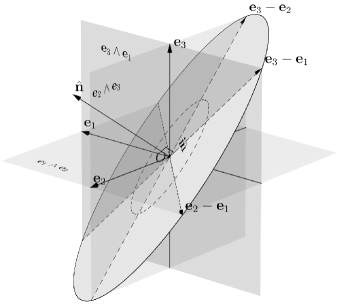
Figure 1. The unit bivector $\mathbf{i}\hat{\mathbf{n}}$ (dashed circle) is the normalized sum of the three orthonormal planes $\mathbf{e}_{1}\wedge\mathbf{e}_{2},\mathbf{e}_{2}\wedge\mathbf{e}_{3}$ and $\mathbf{e}_{3}\wedge\mathbf{e}_{1}$.

Overall, the above analysis shows that the bivector $\mathbf{i}\hat{\mathbf{n}}$ plays the role of the imaginary unit in three dimensions. This means that instead of having the three imaginary units, $i,j$ and $k$, in GA we have the normalized sum of all three of them. Therefore, the geometric representation of the pure quaternion $\frac{1}{\sqrt{3}}(i+j+k)$ is an oriented unit plane normal to the vector $\hat{\mathbf{n}}=\frac{1}{\sqrt{3}}(\mathbf{e}_{1}+\mathbf{e}_{2}+\mathbf{e}_{3})$.

Having a geometric interpretation of the unit bivector, we see that (3.6) represents an unnormalized rotor (operator spinor) producing counterclockwise rotations and dilations in the plane $\mathbf{i}\hat{\mathbf{n}}$. This geometric interpretation is more transparent and intuitive than in the quaternion algebra $\mathbb{H}$, where the imaginary part of (3.1) $\Im(q)$ is interpreted as a vector of $\mathbb{R}^{3}$ having negative square [16].

4. Two-State Quantum Systems in Geometric Algebra

4.1. States and Operators

In GA the classical spinor $|{\psi}\rangle=c_{+}|{+}\rangle+c_{-}|{-}\rangle$ (see the Appendix), can be considered as the representation of an element of the minimal left ideal $S$ of $\mathcal{G}_{3}$. The elements of $S$ are of the form $Af$ where $A\in\mathcal{G}_{3}^{+}$ and $f$ is a primitive idempotent. Therefore, $|{\psi}\rangle$ maps to the algebraic spinor $\Psi$

$$|{\psi}\rangle\leftrightarrow\Psi=\psi_{+}f,$$ (4.1)

where $\psi_{+}$ can be written in terms of the elements of $\mathcal{G}_{3}^{+}$

$$\psi_{+}=a_{0}+a_{1}\mathbf{e}_{23}+a_{2}\mathbf{e}_{31}+a_{3}\mathbf{e}_{12}.$$ (4.2)

Therefore, according to (3.2) $\psi_{+}$ is a quaternion. Furthermore, due to the normalization condition of classical spinors $(\left\langle{\psi}|{\psi}\right\rangle=1)$, we require that $\psi_{+}\tilde{\psi}_{+}=\sum_{i=0}^{3}a_{i}^{2}=1$, hence $\psi_{+}$ must be a unit quaternion or rotor.

We now explain why (4.1) corresponds precisely to the classical spinor $|{\psi}\rangle$. First, note that $\psi_{+}$ can be written as

$$\psi_{+}=(a_{0}+a_{3}\mathbf{e}_{12})+(-a_{2}-a_{1}\mathbf{e}_{12})\boldsymbol{e}_{13}.$$ (4.3)

Now we select the $z$ axis arbitrarily as the quantization direction, meaning that $f=\frac{1}{2}(1+\mathbf{e}_{3})$. Therefore

$$\Psi=(a_{0}+a_{3}\mathbf{i})f+(-a_{2}+a_{1}\mathbf{i})\mathbf{e}_{1}f,$$ (4.4)

were we have used the “Pacwoman property” $\mathbf{e}_{3}f=f$ [17]. Comparing (4.4) with (5.1) we have the correspondences [3]

$$\begin{split}&c_{+}\leftrightarrow\mathfrak{c}_{+}=a_{0}+a_{3}\mathbf{i},\quad c_{-}\leftrightarrow\mathfrak{c}_{-}=-a_{2}+a_{1}\mathbf{i}\\ &|{+}\rangle\leftrightarrow\epsilon_{+}=f,\quad|{-}\rangle\leftrightarrow\epsilon_{-}=\mathbf{e}_{1}f\\ \ &|{\psi}\rangle\leftrightarrow\Psi=\mathfrak{c}_{+}\epsilon_{+}+\mathfrak{c}_{-}\epsilon_{-}.\end{split}$$ (4.5)

Note that $\mathfrak{c}_{+},\mathfrak{c}_{-}\in\text{Cen}(\mathcal{G}_{3})$, hence they commute with all the multivectors of $\mathcal{G}_{3}$. Additionally, we also need the involutions

$$\begin{split}&c_{+}^{*}\leftrightarrow\tilde{\mathfrak{c}}_{+}=a_{0}-a_{3}\mathbf{i},\quad c_{-}^{*}\leftrightarrow\tilde{\mathfrak{c}}_{-}=-a_{2}-a_{1}\mathbf{i}\\ &\langle{+}|\leftrightarrow\tilde{\epsilon}_{+}=\epsilon_{+},\quad\langle{-}|\leftrightarrow\tilde{\epsilon}_{-}=f\mathbf{e}_{1}\\ \ &\langle{\psi}|\leftrightarrow\tilde{\Psi}=\tilde{\mathfrak{c}}_{+}\epsilon_{+}+\tilde{\mathfrak{c}}_{-}\tilde{\epsilon}_{-},\end{split}$$ (4.6)

where ^∗ and ^∼ are the complex conjugation and reversion, respectively.

Finally, the quantum inner product of the two orthonormal states $|{+}\rangle$ and $|{-}\rangle$ of the Hilbert space are written in $\mathcal{G}_{3}$ as follows

$$\begin{split}\langle+|+\rangle\leftrightarrow 2\left\langle{\tilde{\epsilon}_{+}\epsilon_{+}}\right\rangle_{0}=1,\\ \langle-|-\rangle\leftrightarrow 2\left\langle{\tilde{\epsilon}_{-}\epsilon_{-}}\right\rangle_{0}=1,\\ \langle+|-\rangle\leftrightarrow 2\left\langle{\tilde{\epsilon}_{+}\epsilon_{-}}\right\rangle_{0}=0,\\ \langle-|+\rangle\leftrightarrow 2\left\langle{\tilde{\epsilon}_{-}\epsilon_{+}}\right\rangle_{0}=0.\end{split}$$ (4.7)

To continue our discussion, we will see how to write the operators for a TSS in $\mathcal{G}_{3}$. It is well known that the Hamiltonian of a TSS is represented by a linear combination of the Pauli and identity matrices (see the Appendix). In the same way, by making use of the basis (2.7) we claim that any operator in $\mathcal{G}_{3}$ can be written as the superposition

$$H=H_{+}+H_{-},$$ (4.8)

where

$$H_{+} =\sum_{j=0}^{3}h_{j}^{+}\mathbf{e}_{j},\quad\text{where }h_{j}^{+}\in\mathbb{R},$$ (4.9)

$$H_{-} =\mathbf{i}\sum_{j=0}^{3}h_{j}^{-}\mathbf{e}_{j},\quad\text{where }h_{j}^{-}\in\mathbb{R}.$$ (4.10)

Note that (5.4) is the matrix representation of $H_{+}$, whereas the matrix representation of $H_{-}$ is

$$\hat{H}_{-}=i\begin{pmatrix}h_{0}^{-}+h_{3}^{-}&h_{1}^{-}-ih_{2}^{-}\\ h_{1}^{-}+ih_{2}^{-}&h_{0}^{-}-h_{3}^{-}\end{pmatrix}.$$ (4.11)

Note that this matrix is anti-Hermitian, and is conventionally considered as devoid of physical meaning. However, operators such as (4.11) may have a real spectrum if they are symmetric under the Parity–Time $(\mathscr{PT})$ transformation in non-Hermitian quantum mechanics (NHQM) [18]. NHQM is outside the scope of this paper, therefore we will only consider operators such as (4.9).

4.2. Geometric Algebra of Spin Operators

In quantum mechanics, the spin operators defined as $\hat{S}_{i}=\frac{\hbar}{2}\hat{\sigma}_{i}$ for $i=1,2,3$ obey the commutation relations

$$[\hat{S}_{i},\hat{S}_{j}]=i\hbar\epsilon_{ijk}\hat{S}_{k}.$$ (4.12)

However, due to the isomorphism between the matrix algebra $\text{Mat}(2,\mathbb{C})$ and $\mathcal{G}_{3}$, we have the correspondences

$$\hat{S}_{i}=\frac{1}{2}\hbar\hat{\sigma}_{i}\leftrightarrow\mathbf{S}_{i}=\frac{1}{2}\hbar\mathbf{e}_{i},\quad\text{for }i=1,2,3.$$ (4.13)

Therefore, in $\mathcal{G}_{3}$ the spin operators $\hat{S}_{i}$ become the spin vectors $\mathbf{S}_{i}$. With these equivalences in mind and writing the LHS of (4.12) in terms of the spin vectors, we have

$$\mathbf{S}_{i}\mathbf{S}_{j}-\mathbf{S}_{j}\mathbf{S}_{i}=\frac{1}{4}\hbar^{2}(\mathbf{e}_{ij}-\mathbf{e}_{ji}).$$ (4.14)

Substituting (2.12) in the RHS of the above result, we arrive at the commutator

$$[\mathbf{S}_{i},\mathbf{S}_{j}]=\hbar\epsilon_{ijk}\mathbf{i}\mathbf{S}_{k},$$ (4.15)

which is the GA version of the algebra of spin operators of quantum mechanics, where the role of the imaginary unit in (4.12) has been taken by the pseudoscalar of $\mathcal{G}_{3}$ because (4.15) is a bivector identity.

It is well known that (4.12) extends to total $(\hat{J})$ and orbital $(\hat{L})$ angular momentum operators, respectively. Therefore, (4.15) must extend to the corresponding total and orbital angular momentum vectors. Since in GA the orthogonal components of these operators are all vector quantities, it is not surprising that they must obey the same commutation relations.

4.3. Eigenvalues and Eigenvectors

One of the most important problems in quantum mechanics is to determine the energy eigenvalues and eigenvectors of the Hamiltonian

$$\hat{H}=h_{0}\hat{\sigma}_{0}+h_{1}\hat{\sigma}_{1}+h_{2}\hat{\sigma}_{2}+h_{3}\hat{\sigma}_{3}=\begin{pmatrix}h_{0}+h_{3}&h_{1}-ih_{2}\\ h_{1}+ih_{2}&h_{0}-h_{3}\end{pmatrix},$$ (4.16)

which is a self-adjoint or Hermitian matrix.

The standard method to solve this problem consists in finding the eigenvalues by solving the characteristic equation $\text{det}(\hat{H}-\lambda\hat{\sigma}_{0})=0$. Then we use these eigenvalues to find the eigenvectors by solving the eigenvalue equations $\hat{H}|{\psi}\rangle=\lambda|{\psi}\rangle$. The energy eigenvalues are the entries of the diagonal matrix

$$\hat{H}_{0}=\hat{R}^{-1}\hat{H}\hat{R},$$ (4.17)

where $\hat{R}$ is an invertible matrix built from the eigenvectors of $\hat{H}$.

It is well known that if $\hat{H}$ is diagonalizable, then the eigenvalue problem reduces to the simple form

$$\hat{H}_{0}|{\pm}\rangle=E_{\pm}|{\pm}\rangle,$$ (4.18)

where $E_{\pm}$ and $|{\pm}\rangle$ are the eigenvalues and eigenvectors of the Hamiltonian $\hat{H}$, respectively.

Here, we develop a practical method to solve this problem in GA. Let us start by recalling that the operator $\hat{H}$ is the matrix representation of the multivector (4.9)

$$H=h_{0}+\mathbf{r}=h_{0}+|\mathbf{r}|\hat{\mathbf{r}},$$ (4.19)

where $|\mathbf{r}|=\sqrt{h_{1}^{2}+h_{2}^{2}+h_{3}^{2}}$, $\hat{\mathbf{r}}$ is a unit vector parallel to $\mathbf{r}$, and we have written for simplicity $h_{j}^{+}=h_{j}$. To continue, note that in Mat$(2,\mathbb{C})$ the only diagonal matrix (apart from the identity matrix) is $\hat{\sigma}_{3}$. Therefore, all diagonal matrices of Mat$(2,\mathbb{C})$ must be scalar multiples of $\hat{\sigma}_{3}$.

On the other hand, $\mathbf{r}$ has an arbitrary direction in $\mathcal{G}_{3}$. Hence, in analogy to (4.17), we can always make $\mathbf{r}$ parallel to $\mathbf{e}_{3}$ by rotating the multivector $H$:

$$H_{0}=\tilde{R}HR=h_{0}+|\mathbf{r}|\tilde{R}\hat{\mathbf{r}}R=h_{0}+|\mathbf{r}|\mathbf{e_{3}}.$$ (4.20)

Consequently, the matrix representation of the above equation results in a diagonal matrix

$$\hat{H}_{0}=\begin{pmatrix}h_{0}+|\mathbf{r}|&0\\ 0&h_{0}-|\mathbf{r}|\end{pmatrix},$$ (4.21)

and so we have diagonalized $\hat{H}$ just by rotating the vector part of $H$.

The operator spinor or rotor $R$ introduced in (4.20) can be written in terms of the coefficients $h_{1}$, $h_{2}$ and $h_{3}$ as

$$R=R(\varphi)R(\theta)=\exp\left(-\mathbf{ie}_{3}\varphi/2\right)\exp\left(-\mathbf{ie}_{2}\theta/2\right),$$ (4.22)

where the polar angles are given by

$$\theta=\text{tan}^{-1}\left(\frac{\sqrt{h_{1}^{2}+h_{2}^{2}}}{h_{3}}\right),$$ (4.23)

$$\varphi=\tan^{-1}(\frac{h_{2}}{h_{1}}).$$ (4.24)

Having found $H_{0}$ and due to the equivalences (4.5), the eigenvalue equations in GA can be written as

$$\hat{H}_{0}|{\pm}\rangle=E_{\pm}|{\pm}\rangle\leftrightarrow H_{0}\epsilon_{\pm}=E_{\pm}\epsilon_{\pm}.$$ (4.25)

On the order hand, in order to find the eigenvectors of $\hat{H}$, note that the vector part of (4.19) has a direction given by the unit vector $\hat{\mathbf{r}}=\sin\theta\cos\varphi\mathbf{e}_{1}+\sin\theta\sin\varphi\mathbf{e}_{2}+\cos\theta\mathbf{e}_{3}$. Therefore, we may proceed in the same way that the eigenvectors of the spin operator in the arbitrary direction $\mathbf{\hat{n}}$ are found in quantum mechanics, see, for example, [19, Ch. 3].

Suppose that at $t=0$ the classical spinor (5.1) is in the up state, $|{\psi(t=0)}\rangle=|{+}\rangle$. Then, using (4.5) yields $\mathfrak{c}_{+}=1$ and $\mathfrak{c}_{-}=0$, and hence $\Psi(t=0)=\Psi_{+}=\epsilon_{+}$. Now we perform two successive rotations $R(\theta)$ and $R(\varphi)$ on $\Psi_{+}$:

$$\Psi_{\hat{\mathbf{r}}+}=R(\varphi)R(\theta)\Psi_{+}=\exp\left(-\mathbf{ie}_{3}\varphi/2\right)\exp\left(-\mathbf{ie}_{2}\theta/2\right)\epsilon_{+}.$$ (4.26)

The algebraic spinor $\Psi_{\hat{\mathbf{r}}+}$ corresponds to one of the eigenvectors of $\hat{H}$. The other algebraic spinor $\Psi_{\hat{\mathbf{r}}-}$ can be found by rotating $\Psi_{+}$ again, but this time we change $R(\theta)$ to $R(\theta+\pi)$

$$\Psi_{\hat{\mathbf{r}}-}=R(\varphi)R(\theta+\pi)\Psi_{+}=\exp\left(-\mathbf{ie}_{3}\varphi/2\right)\exp\left(-\mathbf{ie}_{2}(\theta/2+\pi/2)\right)\epsilon_{+}.$$ (4.27)

The algebraic spinors $\Psi_{\hat{\mathbf{r}}+}$ and $\Psi_{\hat{\mathbf{r}}-}$ are orthonormal as required.

With the above equivalences, the eigenvalue equations $H\Psi_{\hat{\mathbf{r}}\pm}=E_{\pm}\Psi_{\hat{\mathbf{r}}\pm}$ become

$$\begin{split}H\Psi_{\hat{\mathbf{r}}\pm}&=(h_{0}+|\mathbf{r}|\hat{\mathbf{r}})\Psi_{\hat{\mathbf{r}}\pm}\\ &=(h_{0}\pm|\mathbf{r}|)\Psi_{\hat{\mathbf{r}}\pm}.\end{split}$$ (4.28)

Example.

Let $\hat{H}=a(\hat{\sigma}_{1}+\hat{\sigma}_{3})$ be the Hamiltonian operator for a TLS, where $a$ is a real constant having the dimensions of energy. The problem is to find the corresponding energy eigenvalues and energy eigenvectors as linear combinations of the up and down states.

In order to solve this problem within $\mathcal{G}_{3}$, we begin by writing the operator $\hat{H}$ as $H=a(\mathbf{e}_{1}+\mathbf{e}_{3})$. Using Equations (4.23) and (4.24) we have $\varphi=0$ and $\theta=\pi/4$. Hence the rotor which makes $H$ parallel to $\mathbf{e}_{3}$ is given by (4.22)

$$R=\exp\left(-\mathbf{ie}_{2}\pi/8\right).$$ (4.29)

Now, the rotated Hamiltonian becomes

$$H_{0}=\tilde{R}HR=a\sqrt{2}\mathbf{e}_{3}.$$ (4.30)

The matrix representation of this result reveals the two eigenvalues of $\hat{H}$:

$$\hat{H}_{0}=\begin{pmatrix}a\sqrt{2}&0\\ 0&-a\sqrt{2}\end{pmatrix}.$$ (4.31)

On the other hand, using (4.26) and (4.27), the algebraic spinors associated to $H$ are

$$\Psi_{\hat{\mathbf{r}}+}= \exp\left(-\mathbf{ie}_{2}\pi/8\right)\epsilon_{+},$$ (4.32)

$$\Psi_{\hat{\mathbf{r}}-}= \exp\left(-\mathbf{ie}_{2}5\pi/8\right)\epsilon_{+},$$ (4.33)

from which we can easily calculate their matrix representations, see Problem 1.10 of [19],

$$|{\Psi_{\hat{\mathbf{r}}+}}\rangle= \begin{pmatrix}\frac{\sqrt{2+\sqrt{2}}}{2}&0\\ \frac{\sqrt{2-\sqrt{2}}}{2}&0\end{pmatrix}$$ (4.34)

$$|{\Psi_{\hat{\mathbf{r}}-}}\rangle= \begin{pmatrix}-\frac{\sqrt{2-\sqrt{2}}}{2}&0\\ \frac{\sqrt{2+\sqrt{2}}}{2}&0\end{pmatrix}.$$ (4.35)

4.4. A Spin-$1/2$ Particle Interacting with an External Magnetic Field

In standard quantum mechanics, the Hamiltonian of a non-relativistic particle interacting with an external magnetic field $\mathbf{B}$ is given by

$$\hat{H}=-\frac{q\hbar}{2m}\boldsymbol{\sigma}\cdot\mathbf{B},$$ (4.36)

where $q$ is the charge of the particle, $m$ is its mass and $\hbar$ is the reduced Planck’s constant. Recalling that $\boldsymbol{\sigma}\cdot\mathbf{B}$ is just a short hand for $\hat{\sigma}_{1}B_{1}+\hat{\sigma}_{2}B_{2}+\hat{\sigma}_{3}B_{3}$, we write (4.36) explicitly as

$$\hat{H}=-\frac{q\hbar}{2m}(B_{1}\hat{\sigma}_{1}+B_{2}\hat{\sigma}_{2}+B_{3}\hat{\sigma}_{3}).$$

Note that this equation is similar to the matrix representation of the multivector (4.9) except for the term $h_{0}$, which only changes the reference level of the energy eigenvalues of (4.36). Therefore, in $\mathcal{G}_{3}$ this Hamiltonian can be readily written down as

$$H=-\frac{q\hbar}{2m}\left(B_{1}\mathbf{e}_{1}+B_{2}\mathbf{e}_{2}+B_{3}\mathbf{e}_{3}\right)=-\frac{q\hbar}{2m}\mathbf{B},$$ (4.37)

representing an arbitrary vector of $\mathcal{G}_{3}$.

We now proceed to discuss the dynamics of the state vector wich is described by the time-dependent Schrödinger equation, (see the Appendix)

$$\frac{\mathrm{d}|{\psi}\rangle}{\mathrm{d}t}=-\frac{1}{\hbar}(i\hat{H})|{\psi}\rangle.$$ (4.38)

This equation is straightforwardly translated to $\mathcal{G}_{3}$ as

$$\frac{\mathrm{d}\Psi}{\mathrm{d}t}=-\frac{1}{\hbar}(\mathbf{i}H)\Psi,$$ (4.39)

where we have used (4.1), replaced the imaginary unit $i$ by the pseudoscalar $\mathbf{i}$, and the Hamiltonian (4.36) by the multivector (4.37). Note that the product $(\mathbf{i}H)\Psi$ on the RHS of (4.39) will always remain in $\mathcal{G}_{3}^{+}f$ since $\Psi$ is a minimal left ideal. Therefore, there is no need to multiply the RHS of (4.39) by $\mathbf{e}_{3}$ in order to ensure that the resulting multivector will remain in $\mathcal{G}_{3}^{+}$, as discussed previously in [11].

Now, if the vector $H$ is time independent (constant magnetic field), Equation (4.39) can be easily integrated, yielding

$$\Psi(t)=\exp{\left(-\frac{\mathbf{i}Ht}{\hbar}\right)}{\Psi}(0).$$ (4.40)

Note that (5.6) is the matrix representation of (4.40) due to the isomorphism $G_{3}^{+}f\simeq\mathbb{C}^{2}$. Hence, we have the mapping

$$\hat{U}\leftrightarrow U=\exp{\left(-\frac{\mathbf{i}Ht}{\hbar}\right)}.$$ (4.41)

Thus, in $\mathcal{G}_{3}$ the evolution operator $\hat{U}$ is the matrix representation of the rotor $U=\exp{(-\frac{\mathbf{i}Ht}{\hbar})}\in\mathcal{G}_{3}^{+}$, which is a rotor since the factor $\mathbf{i}H$ in its exponent is a bivector. Writing $U$ in terms of (4.37) gives us

$$U=\exp{\left(\mathbf{i}\hat{\mathbf{B}}\frac{\alpha}{2}\right)},$$ (4.42)

where $\hat{\mathbf{B}}$ is a unit vector parallel to ${\mathbf{B}}$ and $\alpha=\frac{q|\mathbf{B}|t}{m}$.

4.5. Expectation Values

Other quantities of interest in quantum mechanics are the expectation values of the Hermitian operator (4.16), conventionally computed by

$$\langle\hat{H}\rangle=\langle\psi|\hat{H}|\psi\rangle.$$ (4.43)

Using the equivalences (4.5), the above definition corresponds to taking the scalar part of the product $\tilde{\Psi}H\Psi$ and multiplying it by 2. See, for example, [2]

$$\langle H\rangle=2\langle\tilde{\Psi}H\Psi\rangle_{0}.$$ (4.44)

Example (Spin Precession).

As an application of (4.44), we will compute the expectation values of the spin operators $\hat{S}_{i}=(\hbar/2)\hat{\sigma}_{i}$. As we have seen in (4.13), $\hat{S}_{i}$ corresponds to the spin vectors $\mathbf{S}_{i}=(\hbar/2)\mathbf{e}_{i}$ ($i=1,2,3$).

Recalling that $\Psi(t)$ is given by (4.40), letting $\Psi(0)=\text{exp}(-\mathbf{ie}_{2}\theta/2)\epsilon_{+}$, and setting $\hat{\mathbf{B}}=\mathbf{e}_{3}$ in (4.42), we have

$$\Psi(t)=U\Psi(0)=\text{exp}(\mathbf{ie}_{3}\frac{\alpha}{2})\text{exp}(-\mathbf{ie}_{2}\frac{\theta}{2})\epsilon_{+}.$$ (4.45)

Thus, the expectation value of $\mathbf{S}_{1}$ becomes

$$\langle\mathbf{S}_{1}\rangle =\hbar\langle\tilde{\Psi}(t)\mathbf{e}_{1}\Psi(t)\rangle_{0}$$ (4.46)

$$=\hbar\langle\epsilon_{+}\text{exp}(\mathbf{ie}_{2}\frac{\theta}{2})\text{exp}(-\mathbf{ie}_{3}\frac{\alpha}{2})\mathbf{e}_{1}\text{exp}(\mathbf{ie}_{3}\frac{\alpha}{2})\text{exp}(-\mathbf{ie}_{2}\frac{\theta}{2})\epsilon_{+}\rangle_{0}$$ (4.47)

$$=\hbar\langle\sin(\theta)\cos(\omega t)\epsilon_{+}+\cos(\theta)\cos(\omega t)\epsilon_{+}\epsilon_{-}+\sin(\omega t)\epsilon_{+}\mathbf{e}_{2}\epsilon_{+}\rangle_{0}$$ (4.48)

$$=\frac{\hbar}{2}\sin(\theta)\cos(\omega t),$$ (4.49)

since $\epsilon_{+}\epsilon_{-}=\epsilon_{+}\mathbf{e}_{2}\epsilon_{+}=0$ and $\langle\epsilon_{+}\rangle_{0}=1/2$.

In the same fashion, the expectation values of $\mathbf{S}_{2}$ and $\mathbf{S}_{3}$ are

$$\langle\mathbf{S}_{2}\rangle =-\frac{\hbar}{2}\sin(\theta)\sin(\omega t),$$ (4.50)

$$\langle\mathbf{S}_{3}\rangle =\frac{\hbar}{2}\cos(\theta),$$ (4.51)

which describes the precession of $\langle\mathbf{S}\rangle$ in the plane $\mathbf{ie}_{3}$ at the Larmor frequency $\omega=qB_{3}/m$.

Alternatively, we obtain all the components of the spin vector $\mathbf{S}$ easily using the operator spinor $\psi_{+}=\text{exp}(\mathbf{ie}_{3}\frac{\alpha}{2})\text{exp}(-\mathbf{ie}_{2}\frac{\theta}{2})$ acting on $\mathbf{S}_{3}$ as follows, see [2] for more details.

$$\mathbf{S}=\psi_{+}\mathbf{S}_{3}\tilde{\psi}_{+}=\frac{\hbar}{2}(\sin(\theta)\cos(\omega t)\mathbf{e}_{1}-\sin(\theta)\sin(\omega t)\mathbf{e}_{2}+\cos(\theta)\mathbf{e}_{3}).$$ (4.52)

Therefore, the expectation values $\langle\mathbf{S}_{i}\rangle$ can be readily obtained as

$$\langle\mathbf{S}_{i}\rangle=\mathbf{S}\cdot\mathbf{e}_{i},\quad i=1,2,3.$$ (4.53)

4.6. Probability

Conventionally, if $\hat{A}$ is a Hermitian operator with a non-degenerate discrete spectrum with eigenvalues $a_{n}$, then there is a unique eigenvector $|{u_{n}}\rangle$ associated to each eigenvalue $a_{n}$. Since the set of $|{u_{n}}\rangle$ constitutes a basis, then $|{\psi(t)}\rangle=\sum_{n}c_{n}|{u_{n}}\rangle$. Therefore, the probability of finding $a_{n}$ when $\hat{A}$ is measured is given by [20]

$$P(a_{n})=|c_{n}|^{2}=\langle u_{n}|\psi(t)\rangle\langle\psi(t)|u_{n}\rangle.$$ (4.54)

Again, using the equivalences (4.5), and (4.6), the translation of (4.54) to $\mathcal{G}_{3}$ yields

$$P(a_{n})=2\langle\tilde{u}_{n}\Psi(t)\tilde{\Psi}(t)u_{n}\rangle_{0}.$$ (4.55)

Example (Rabi Formula).

In the preceding example, the direction of the magnetic field was along the positive $z$-axis. Now, imagine that the spin is initially in the eigenstate $|{+}\rangle$ of $\hat{S}_{3}$, and then we set the magnetic field in an arbitrary direction $\mathbf{B}=B_{1}\mathbf{e}_{1}+B_{2}\mathbf{e}_{2}+B_{3}\mathbf{e}_{3}$. We will now see how the probability $P_{+-}(t)$ of finding the spin in the eigenstate $|{-}\rangle$ of $\hat{S}_{3}$ at time $t$ is calculated in GA.

First, according to (5.1), the state vector is given in terms of the basis $|{\pm}\rangle$ of $\hat{S}_{3}$ by $|{\psi}\rangle=c_{+}|{+}\rangle+c_{-}|{-}\rangle$. Now, if the spin is initially in the eigenstate $|{+}\rangle$ of $\hat{S}_{3}$, then $c_{+}=1$ and $c_{-}=0$; therefore, using (4.5), the algebraic spinor at time $t=0$ becomes $\Psi(0)=\epsilon_{+}$. Consequently, at time $t$ we have

$$\Psi(t)=U\Psi(0)=\exp\left(\frac{\mathbf{i}(B_{1}\mathbf{e}_{1}+B_{2}\mathbf{e}_{2}+B_{3}\mathbf{e}_{3})}{\sqrt{B_{1}^{2}+B_{2}^{2}+B_{3}^{2}}}\frac{\alpha}{2}\right)\epsilon_{+},$$ (4.56)

where we have written explicitly the rotor (4.42) in terms of the arbitrary field $\mathbf{B}$.

Having $\Psi(t)$, now we can find the probability $P_{+-}(t)$ using the formula (4.55):

$$P_{+-}(t)=2\langle\tilde{\epsilon}_{-}\Psi(t)\tilde{\Psi}(t)\epsilon_{-}\rangle_{0}=2\langle\tilde{\epsilon}_{-}(U\epsilon_{+}\tilde{U})\epsilon_{-}\rangle_{0}.$$ (4.57)

Expanding the term in parentheses in the RHS of (4.57), we have

$$U\epsilon_{+}\tilde{U}=\frac{1}{2}\left(1+\mathbf{u}(t)\right),$$ (4.58)

where $\mathbf{u}(t)$ is given by

$$\begin{split}\mathbf{u}(t)&=U\mathbf{e}_{3}\tilde{U}=\frac{1}{|\mathbf{B}|}\left(B_{1}\cos\theta(1-\cos\alpha)+B_{2}\sin\alpha\right)\mathbf{e}_{1}\\ &+\frac{1}{|\mathbf{B}|}\left(B_{2}\cos\theta(1-\cos\alpha)-B_{1}\sin\alpha\right)\mathbf{e}_{2}+\left(\cos^{2}\theta+\sin^{2}\theta\cos\alpha\right)\mathbf{e}_{3}.\end{split}$$ (4.59)

Here $\theta$ is the angle between the field $\mathbf{B}$ and $\mathbf{e}_{3}$, see Figure 2.

Using this result, the probability $P_{+-}(t)$ reduces to

$$P_{+-}(t)=2\langle\frac{1}{2}\left(1-\cos^{2}\theta-\sin^{2}\theta\cos\alpha\right)\epsilon_{+}\rangle_{0}.$$ (4.60)

Finally, we can simplify this expression by writing $1=\cos^{2}\theta+\sin^{2}\theta$ and $\alpha=\omega t$:

$$P_{+-}(t)=\frac{1}{2}\sin^{2}\theta\left(1-\cos\omega t\right).$$ (4.61)

Equation (4.61) is best known as Rabi’s formula. It gives us the probability of finding the system at time $t$ in the eigenstate $\epsilon_{-}$.

The geometric interpretation of this result is shown in Figure 2. If we define $\mathbf{S}_{u}(t)=(\hbar/2)\mathbf{u}(t)$, then according to (4.59), at time $t=0$, $\mathbf{S}_{u}(t)$ reduces to

$$\mathbf{S}_{u}(0)=\frac{\hbar}{2}\mathbf{e}_{3}.$$ (4.62)

Therefore, initially the spin vector is parallel to $\mathbf{e}_{3}$. Then as times goes on, $\left\langle{\mathbf{S}_{u}(t)}\right\rangle$ precesses clockwise in the plane $\mathbf{i}\hat{\mathbf{B}}$ at the Larmor frequency $\omega=\frac{q|\mathbf{B}|}{m}$. See [20, Ch, IV] for an alternative geometric interpretation of Rabi’s formula.

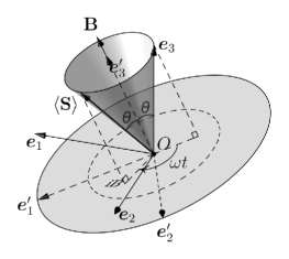
Figure 2. Geometric interpretation of spin precession for an arbitrary field $\mathbf{B}$.

5. Summary and Conclusions

We have studied TSS entirely within the geometric algebra of three dimensional space. In this approach, the mathematical tools conventionally used to describe TSS, namely the complex numbers, linear vector spaces, eigenvalues, eigenvectors, etc., are unified into a single algebra. This unification supports the claim that “GA provides a unified language for the whole physics that is conceptually and computationally superior to alternative systems in every application domain” [21].

Writing the Pauli spinors and the self-adjoint operators of conventional quantum mechanics as elements of $\mathcal{G}_{3}$, we have computed the energy eigenvalues and eigenvectors of an arbitrary TSS. Also, the geometric interpretation of the Hermitian operators of the TSS enables us to diagonalize them just by rotating their vector part. In fact, we do not have to use (4.20) to find the correspondig diagonal matrix, because rotors preserve the norm of a vector, so it suffices to compute their norm and then multiply the result by $\mathbf{e}_{3}$. This geometric interpretation is not present in the conventional theory.

We also revisited the problem of a spin-$1/2$ particle interacting with an external magnetic field, where the interaction Hamiltonian of this system has been interpreted as a vector of $\mathcal{G}_{3}$. We have shown that the time evolution of the state vector reduces to the single side transformation law of algebraic spinors. This also shows that the time evolution operator of quantum mechanics is represented as an operator spinor of $\mathcal{G}_{3}$. We have also computed the expectation values and transition probabilities of this system, obtaining the same results as the conventional theory. However, the algebraic approach reveals the underlying geometry of the probability transition $P_{+-}(t)$, which reduces to the Larmor precession in the arbitrary plane $\mathbf{i}\hat{\mathbf{B}}$.

Lastly, we have rewritten the algebra of spin operators (4.12) as the geometric algebra of the spin vectors (4.15) where the pseudoscalar of $\mathcal{G}_{3}$ plays the role of the imaginary unit $\sqrt{-1}$. However, whereas in the conventional theory this imaginary unit is introduced ad hoc to ensure that the commutator of the LHS of (4.12) results in a Hermitian matrix, the pseudoscalar $\mathbf{i}$ sends the spin vector $\mathbf{S}_{k}$, up to a multiplicative constant, to the spin bivector $\mathbf{S}_{i}\mathbf{S}_{j}$ via Hodge duality. Therefore, the algebra of spin vectors (4.15) results from the anticommutativity of the geometric product.

Acknowledgment

This work was supported by the Huiracocha grant from the Graduate School of the Pontificia Universidad Católica del Perú.

Appendix

Two-State Quantum Systems in a Hilbert Space

Conventionally, a two-state quantum system is mathematically encoded using a two-dimensional complex Hilbert space $\mathcal{H}_{2}$. In this space, the TSS, represented by the state vector or classical spinor $|{\psi}\rangle$, can be written as the superposition of two orthonormal states $|{+}\rangle$ and $|{-}\rangle$, with complex coefficients $c_{+}$ and $c_{-}$:

$$|{\psi}\rangle=c_{+}|{+}\rangle+c_{-}|{-}\rangle.$$ (5.1)

This state vector contains all the information about the quantum system and satisfies the normalization condition $\left\langle{\psi}|{\psi}\right\rangle=1$, implying that $|c_{+}|^{2}+|c_{-}|^{2}=1$. Here the complex coefficients are called probability amplitudes.

On the other hand, in order to perform measurements on a quantum system, it is necessary to introduce a set of operators acting on the quantum states described by Equation (5.1). These operators can be written as linear combinations of the following $2\times 2$ Hermitian matrices.

$$\hat{\sigma}_{0}=\begin{pmatrix}1&0\\ 0&1\end{pmatrix},\quad\hat{\sigma}_{1}=\begin{pmatrix}0&1\\ 1&0\end{pmatrix},\quad\hat{\sigma}_{2}=\begin{pmatrix}0&-i\\ i&0\end{pmatrix},\quad\hat{\sigma}_{3}=\begin{pmatrix}1&0\\ 0&-1\end{pmatrix}$$ (5.2)

Here, the identity matrix $\hat{\sigma}_{0}$ together with the Pauli matrices $\hat{\sigma}_{1},\hat{\sigma}_{2}$, and $\hat{\sigma}_{3}$ satisfy the well-known relation

$$\hat{\sigma}_{l}\hat{\sigma}_{m}=\hat{\sigma}_{0}\delta_{lm}+i\epsilon_{lmn}\hat{\sigma}_{n},$$ (5.3)

which is the matrix representation of (2.11). Consequently, any operator can be written as the sum

$$\hat{H}=h_{0}\hat{\sigma}_{0}+h_{1}\hat{\sigma}_{1}+h_{2}\hat{\sigma}_{2}+h_{3}\hat{\sigma}_{3}.$$ (5.4)

In addition, since $\hat{H}$ is a Hermitian matrix, the coeficients $h_{k}$, $(k=0,\ldots,3)$ must be real numbers.

Finally, the dynamics of the state vector is described by the Schrödinger equation

$$i\hbar\frac{\partial|{\psi}\rangle}{\partial t}=\hat{H}|{\psi}\rangle,$$ (5.5)

where $\hat{H}$ represents the Hamiltonian of the TSS. If this Hamiltonian is time independent, then Equation (5.5) shows that the state of the system at any time $t$ can be obtained by the evolution operator $\hat{U}=~{}\exp(-i\hat{H}t/\hbar)$ acting on the initial state $|{\psi_{0}}\rangle$, i.e.

$$|{\psi(t)}\rangle=\hat{U}|{\psi_{0}}\rangle.$$ (5.6)

References

- [1] B.J. Hiley and R.E. Callaghan. Clifford algebras and the Dirac–Bohm quantum Hamilton–Jacobi equation. Foundations of Physics, 42(1):192–208, (2012).
- [2] P. Lounesto. Clifford Algebras and Spinors. Cambridge University Press, (2001).
- [3] J. Vaz and R. da Rocha. An Introduction to Clifford Algebras and Spinors. Oxford University Press, (2016).
- [4] Y.M. Zou. Ideal structure of Clifford algebras. Advances in Applied Clifford Algebras, 19(1):147–153, (2009).
- [5] J.W. Arthur. Understanding Geometric Algebra for Electromagnetic Theory. John Wiley & Sons, Hoboken, New Jersey (2011).
- [6] J. Dressel, K.Y. Bliokh, and F. Nori. Spacetime algebra as a powerful tool for electromagnetism. Physics Reports, 589:1–71, (2015).
- [7] D. Hestenes. Spacetime physics with geometric algebra. American Journal of Physics, 71(7):691–714, (2003).
- [8] A. Lasenby, C. Doran, and S. Gull. Gravity, gauge theories and geometric algebra. Philosophical Transactions of the Royal Society A: Mathematical, Physical and Engineering Sciences, 356(1737):487–582, (1998).
- [9] A.N. Lasenby. Geometric algebra, gravity and gravitational waves. Advances in Applied Clifford Algebras, 29(4), (2019).
- [10] A. Dargys and A. Acus. Calculation of quantum eigens with geometrical algebra rotors. Advances in Applied Clifford Algebras, 27(1):241–253, (2017).
- [11] C. Doran, and A. Lasenby. Geometric Algebra for Physicists. Cambridge University Press, (2003).
- [12] M.R. Francis and A. Kosowsky. The construction of spinors in geometric algebra. Annals of Physics, 317(2):383–409, (2005).
- [13] W.E. Baylis, R. Cabrera, and J.D. Keselica. Quantum/classical interface: Classical geometric origin of fermion spin. Advances in Applied Clifford Algebras, 20(3–4):517–545, (2010).
- [14] C. McKenzie. An Interpretation of Relativistic Spin Entanglement Using Geometric Algebra. (2015). Electronic Theses and Dissertations. 5652. https://scholar.uwindsor.ca/etd/5652
- [15] P. Lounesto and G. P. Wene. Idempotent structure of Clifford algebras. Acta Applicandae Mathematica, 9(3):165–173, Jul (1987).
- [16] J.P. Morais, S. Georgiev, and W. Sprößig. Real Quaternionic Calculus Handbook. Birkhäuser, Basel. (2014).
- [17] W. Baylis. Electrodynamics: A Modern Geometric Approach. Progress in Mathematical Physics. Birkhäuser Boston, (2004).
- [18] C. Bender and S. Boettcher. Real spectra in non-Hermitian Hamiltonians having symmetry. Phys. Rev. Lett., 80:5243–5246, Jun (1998).
- [19] J.J. Sakurai and J. Napolitano. Modern Quantum Mechanics. Addison-Wesley, (2011).
- [20] C. Cohen-Tannoudji, B. Diu, and F. Laloe. Quantum Mechanics. Wiley, (1991).
- [21] D. Hestenes. Oersted medal lecture 2002: Reforming the mathematical language of physics. American Journal of Physics, 71(2):104–121, (2003).